Digital mapping of pesticides bioconcentration by integrating remote sensing techniques and plant uptake model

ABSTRACT

Although pesticides have been widely used worldwide to enhance crop yield and product quality, most pesticides are harmful to the environment and human health. Plants absorb pesticides mainly from air and soil. Therefore, the soil-plant pathway is essential for pesticide absorption. Bioconcentration factor (BCF) has extensively been applied to evaluate potential plant contamination by pesticides from soil. Hence, this study developed a simplified plant transpiration-based plant uptake model (PT-model) to estimate plant pesticides’ BCF from soil based on plant transpiration. Remote sensing techniques were employed to generate spatiotemporal continuous plant transpiration via evapotranspiration. Pesticide BCF mapping was achieved by integrating PT-model with Moderate Resolution Imaging Spectroradiometer (MODIS) remotely sensed data. The results were compared with a verified model driven by relative humidity and air temperature (RA-model), which has been confirmed by findings from previous studies. The estimated BCF was within the boundaries of the RA-model, indicating the simulation’s overall acceptability. In this study, the BCF temporal trend estimated by the proposed method agreed with the RA-model assimilating meteorology datasets, while the spatial distribution was partially inconsistent. Overall, the proposed method generates the spatiotemporal patterns of pesticide BCF with relatively consistent results supported by previous records and findings.

KEYWORDS:

• Pesticide
• bioconcentration factor
• evapotranspiration
• plant uptake model
• remote sensing

1. Introduction

Various pesticides have been excessively applied to control pests, diseases, weeds, and many other aggressors discovered to cause serious adverse effects on crop yield and quality since the nineteenth century; hence their usage has surged since the twentieth century (Calderbank 1989; Akter et al. 2018; Zhang 2018; Bhandari et al. 2020). Although significant advantages have been acquired from the invention and usage of pesticides, environmental pollution, food insecurity risks, and human health issues have emerged consequently due to the high toxicity and intensive use of pesticides in modern agriculture (Pico et al. 2018; Kumari and John 2019; Philippe et al. 2021). Pesticide residues are frequently detected in fruits and other agricultural products. More importantly, several human health issues, such as cancer and reproductive problems, are more likely for farmers and people living in high pesticide application regions (Fantke et al. 2011; Akter et al. 2018; Bhandari et al. 2020). Besides, the excessive application of pesticides has damaged soil structure and destroyed the soil’s ecological balance and environmental biodiversity (Yu, Ying, and Kookana 2009; Pico et al. 2018; Zhang 2018; Tudi et al. 2021).

Air and soil are the primary intermediates during pesticide application (Alamdar et al. 2014; Islam, Huang, and Siciliano 2020; Tudi et al. 2021). Nevertheless, unlike air, soil composition is quite complex and dynamic; these characteristics may lead chemical particles such as pesticides to enter their binding sites, which causes pesticide persistence in soils for quite a long time. For some types of pesticides, the residual periods may take several decades (Calderbank 1989; Sun et al. 2018; Sanchez et al. 2019; Silva et al. 2019; Bhandari et al. 2020). As a result, the soil is the most crucial exposure medium to pesticides. Several studies have proven that the soil-plant pathway is a significant component of plant pesticide-contaminated risk assessment, and pesticide uptake from the soil is one of the primary sources of pesticide residues in plant tissues (Hwang, Zimmerman, and Kim 2018; Xiao, Li, and Fantke 2021).

Bioconcentration factor (BCF), which indicates the ratio of pesticide concentrations in the plant and soil, is applied to evaluate the bioconcentration process that dominates pesticide uptake via plants’ roots from soil (Hwang, Lee, and Kim 2017; Xiao, Li, and Fantke 2021). Nowadays, field measurements and mathematical models are widely applied to investigate the bioconcentration process of pesticides from soil and theoretically predict pesticide concentration in plants (Fantke et al. 2011; Doucette et al. 2018; Li 2020). Field experimental studies are still the most effective method for obtaining the BCF. However, such experiments are time-consuming and require intensive human resources. Compared to field experiments, models efficiently explain the processes and save time. Therefore, several models have been developed to describe, predict, and simulate plant uptake processes of pesticides and other organic chemicals (Köhne, Köhne, and Šimůnek 2009; Juraske et al. 2009; Hwang, Lee, and Kim 2017; Li 2020).

Numerous models have been developed focusing on the pesticide exchange in the plant-environment system, and the proposed models mainly covered pesticide uptake by plants from the soil in terms of chemical properties and quantitative structural factors (Hsu et al., 1990; Trapp and Matthies 1995; Trapp 2003; Trapp et al. 2007; Rein et al., 2011; Hwang, Lee, and Kim 2017; Li 2020). Briggs, Bromilow, and Evans (1982) used the octanol–water partition coefficient ($K_{OW}$) as a chemical property to estimate chemical uptake by plant roots and stems from the soil. Since then, various models have also been developed. The transpiration stream concentration factor (TSCF) is another significant achievement in plant uptake modeling (Hwang, Lee, and Kim 2017). Trapp and Matthies (1995) developed a one-compartment model for describing the uptake from soil or air only considering a single part of the plant (e.g. leaf, root, or fruit). Similarly, most recently studied methods and multi-compartment models were developed based on the one-compartment modeling concept (Collins and Finnegan 2010; Li 2020).

Pesticides’ BCF spatiotemporal patterns are significant to their proper use and risk assessment (Yao et al. 2006; Miao et al. 2018; Li 2020). Nevertheless, the field experiments and models mentioned above are in overall point-based estimations, hence unable to monitor the distribution trends of pesticides BCF. Various studies have found that the spatiotemporal patterns of plant uptake of pesticides from the soil heavily depend on several ecological and meteorological factors, such as plant transpiration, vegetation vigor, health, temperature, and humidity (Yao et al. 2006; Li 2020). As a result, under continuously distributed spatiotemporal conditions, geographical and meteorological factors are involved in plant uptake modeling when mapping pesticides BCF. This study mainly focuses on applying plant transpiration to a simplified plant uptake model for mapping pesticides BCF.

Plant transpiration and soil evaporation are the two main evapotranspiration (ET) components. As ET depicts a significant complex part of the global hydrological cycle, the monitoring of ET critically emphasizes global water management and crop water requirements. Nevertheless, ET cannot be measured directly yet inferred through energy budget methods (Kool et al. 2014; Bhattarai and Wagle 2021). Over the past decades, several methods have been developed to estimate ET from different climatic and meteorological features (Velpuri et al. 2013; Kool et al. 2014). However, these energy budget methods are station-observation-based, making measuring and continuously predicting ET spatial variation challenging, particularly at large scales. Remote sensing techniques have been widely applied to retrieve ET at regional and global scales, owing to its expanse coverage, high resolution, free availability, and reasonable accuracy (Velpuri et al. 2013; Zhang, Kimball, and Running 2016; Bhattarai and Wagle 2021).

Plant transpiration describes water movement from the soil to the atmosphere through plant roots, stems, and leaves. It plays a vital role in the bioconcentration processes (Niu et al. 2020). Plant transpiration can be measured mainly using the Sap flow, Charmer, and Biomass-PTs method (Xu et al. 2016; Li et al. 2019). However, plant transpiration cannot be obtained directly from remotely sensed data. Models have been developed to separately estimate plant transpiration and soil evaporation (Li et al. 2019). In regions with full or high canopy cover, ET is mainly determined by plant transpiration, while in sparsely vegetated areas, soil evaporation constitutes a significant fraction of ET (Li et al. 2019). Previous studies have indicated that plant transpiration highly depends on vegetation coverage and the crop coefficient, especially in agricultural areas. Consequently, plant transpiration can be determined by indirectly integrating ET and vegetated parameters through remote sensing techniques (Neale et al., 2015).

We choose atrazine as the typical pesticide to evaluate the proposed method’s applicability and simulate the spatiotemporal patterns of the atrazine BCF over the mainland of the U.S.A. As atrazine is one of the most widely used pesticides in the U.S.A., especially for corn and sorghum fields for weeds control, it was applied directly to the soil, mainly during pre-planting or pre-emergence periods over around three-fourths of the corn and sorghum fields (Singh et al. 2018; de Albuquerque et al. 2020). Atrazine may exist in the soil for quite a long time and is also a significant aquatic micropollutant (de Albuquerque et al. 2020). As a result, the transpiration process dominates its absorption from the soil. Atrazine may damage the human and animal endocrine systems and introduce cytotoxicity in living cells (Singh et al. 2018; Xu et al. 2019; Tulcan et al. 2021). Estimating the continuous spatiotemporal potential of plant atrazine uptake from the soil is further significant to risk assessment and environmental protection.

This study developed a plant transpiration-based simplified plant uptake model (PT-model) to simulate and map the plant uptake of pesticides from soil. Spatiotemporal continuous plant transpiration observations obtained by integrating remote sensing ET and a radiometric vegetation index were incorporated into the proposed model for atrazine BCF estimation. The results produced by the PT-model were compared with a relative humidity and air temperature-based spatiotemporal plant uptake model (RA-model) and confirmed by literature-converted data from previous studies.

2. Materials and methods

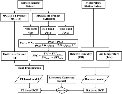
This study developed a simplified plant uptake model (PT-model) plant transpiration-based to calculate the BCF (the ratio of the pesticide concentration in the plant ($C_L$) to the pesticide concentration in the soil ($C_S$); BCF = $C_L/C_S$). BCF identifies the potential pesticide bioconcentration. BCF can be applied to estimate bioconcentration by combining pesticide dosage, soil degradation, etc. It is important to note that BCF is an indicator of the potential of pesticide bioconcentration, and it’s tough to measure the actual value of BCF through experiments. Remote sensing techniques were combined with the PT-model to map the spatiotemporal patterns of plant pesticide (Atrazine) uptake from the soil, as illustrated in Figure 1. The proposed methodology in this study consists of three parts: (1) the traditional one-compart plant uptake model was simplified based on the steady-state mass balance equation, BCF can be estimated through the simplified model based on the plant transpiration and other chemical properties; (2) spatiotemporal variation of plant transpiration was generated through MODIS ET data and a vegetation index retrieved from MODIS data expressed in surface reflectance; (3) plant transpiration datasets were integrated with the PT-model to generate BCF, spatiotemporal patterns of BCF were simulated and compared to previous confirmed modeling findings.

Figure 1. Workflow chart of the proposed methodology.

2.1. Simplified plant transpiration-based plant uptake model

The one-compartment model developed by Trapp and Matthies (1995) simulates the uptake of organic pollutants (pesticides) by plants from the soil, and the original model can be expressed as follows: (1) $\begin{array}{c}{\displaystyle \frac{d(C_L{M}_L)}{dt}=Q_{L}TSCF{C}_W-A_{L}g{\displaystyle \frac{C_L}{K_{LA}}-{\lambda }_L{C}_L{M}_L}}\end{array}$(1) where $C_L$ indicates the pesticide concentration in the plant, the leaf part is mainly considered in this study; $M_L$ is the leaf mass; $t$ is the time period; $Q_L$ is the leaf transpiration rate, $A_L$ is the leaf area, the ration between $Q_L$ and $A_L$ can be used to represent plant transpiration; $TSCF$ is the transpiration stream concentration factor, describing the transpiration of pesticides from roots to other compartments of the plant and can be calculated through $K_{OW}$; $K_{LA}$ is the leaf-air partition coefficient, which represents the gaseous exchange between leaves and the atmosphere and can be estimated based on the ratio between the leaf-water partition coefficient ($K_{LW}$) and Henry’s constant ($K_{AW}$); ${\lambda }_L$ indicates the total pesticide loss rate in the leaves, depending on the photodegradation, plant metabolism, and dilution rates due to plant growth (Hsu et al., 1990; Trapp and Matthies 1995; Hwang, Lee, and Kim 2017); $C_W$ denotes the soil solution and can be estimated through the ratio between the pesticide concentration in soil and the coefficient of soil-water partition, based on the studies of Trapp (2003), Trapp et al. (2007), Rein et al. (2011), and Li (2020). Parameters for the estimations of related factors applied in this study were mainly provided by Fantke et al. (2017), Lewis et al. (2006), Trapp and Matthies (1995) and Trapp et al. (2007).

The newly one-compartment model can be expressed as follows (Li and Ai 2023): (2) $\begin{array}{c}{\displaystyle \frac{d(C_L{M}_L)}{dt}=\left({\displaystyle \frac{TSCF}{K_{SW}}}\right)Q_L{C}_S-A_{L}g{\displaystyle \frac{C_L}{K_{LA}}-{\lambda }_L{C}_L{M}_L}}\end{array}$(2)

A steady-state mass balance condition was assumed to estimate organic pollutants (pesticides) BCF as follows: (3) $\begin{array}{c}{\displaystyle \frac{d(C_L{M}_L)}{dt}=0}\end{array}$(3)

The mass of the plant leaf part can be estimated by the production of leaf area, thickness, and density as presented in equation (4): (4) $\begin{array}{c}{M}_L=A_L{D}_L{\rho }_L\end{array}$(4) where $D_L$, ${\rho }_L$ are the leaf thickness and density, respectively.

The ratio between $Q_L$ and $A_L$ denotes plant transpiration ($PT$) is computed using equation (5): (5) $\begin{array}{c}PT=\left({\displaystyle \frac{Q_L}{A_L}}\right)\end{array}$(5)

The PT-model for bioconcentration factor estimation developed from Li and Ai (2023) can be expressed as follows: (6) $\begin{array}{c}BCF(PT)=PT\left({\displaystyle \frac{\left({\displaystyle \frac{TSCF}{K_{SW}}}\right)}{g\left({\displaystyle \frac{1}{K_{LA}}}\right)+{\lambda }_L{D}_L{\rho }_L}}\right)\end{array}$(6)

2.2. Plant transpiration estimation

Remote sensing observations were applied to estimate plant transpiration and then integrated into the plant transpiration-based model. In this regard, Moderate Resolution Imaging Spectroradiometer (MODIS) datasets were used in this study to obtain the required variables (ET and vegetation index) to retrieve plant transpiration. MODIS is the most critical instrument aboard the Terra and Aqua satellites, which provides global coverage of land, water, and lower atmosphere at various spatial and temporal resolutions. MODIS daily surface reflectance datasets (MOD09) with 500 m spatial resolution and 8-day/500 m ET datasets (MOD16) were used in this research to estimate BCF. The daily remote sensing products were aggregated to 8-day temporal resolution for further analysis.

The MODIS ET retrieval algorithms are conducted based on Penman-Monteith (P-M) equation presented below (Mu et al. 2007; Mu, Zhao, and Running 2011). (7) $\begin{array}{c}\lambda E={\displaystyle \frac{\mathrm{\Delta }(R_n-G)+\left[{\displaystyle \frac{{\rho }_a{C}_p(e_s-e_a)}{r_a}}\right]}{\mathrm{\Delta }+\gamma \left(1+{\displaystyle \frac{r_s}{r_a}}\right)}}\end{array}$(7) where $\lambda E$ is the latent heat flux and $\lambda$ is the latent heat of evaporation; $\mathrm{\Delta }$ is the slope of the saturated vapor pressure curve, $R_n$ is net radiation flux, G is sensible heat flux into the soil, $\gamma$ is psychrometric constant, ${\rho }_a$ is the air density, $C_p$ is the specific heat of dry air at constant pressure, $e_s$ is the mean saturated vapor pressure, $r_a$ is the bulk surface aerodynamic resistance for water vapor, $e_a$ is mean daily ambient vapor pressure and $r_s$ is the canopy surface resistance.

The MOD16 algorithm assimilates land cover type, albedo, leaf area index, and daily meteorological observations from NASA’s Global Modeling and Assimilation Office (GMAO) reanalysis dataset into the P-M equation. It considers the atmospheric drivers and surface energy portioning process to monitor regional and global evapotranspiration variations (Velpuri et al. 2013).

The unit of MODIS-derived ET is mm/8d, the sum of evaporation within the past eight days, while the transpiration unit applied in PT-model is m/d. It must be noted here that the MODIS-derived ET needs to be transformed first using equation (8) presented below: (8) $\begin{array}{c}ET={\displaystyle \frac{E{T}_{MODIS}\ast {10}^{-3}}{8}}\end{array}$(8)

The MODIS ET dataset is mainly composed of soil evaporation and plant transpiration. However, the plant uptake of pesticides from the soil is primarily related to plant transpiration. Therefore, plant transpiration needs to be extracted from ET, considering vegetation coverage. It can be expressed as follows: (9) $\begin{array}{c}PT=ET\ast {\mathrm{\partial }}_v\ast FVC\end{array}$(9) where ${\mathrm{\partial }}_v$ is the ratio of PT to ET with full vegetation cover, $FVC$ is fractional vegetation cover expressed as follows: (10) $\begin{array}{c}FVC={\displaystyle \frac{EVI-EV{I}_{min}}{EV{I}_{max}-EV{I}_{min}}}\end{array}$(10) where $EVI$ is the enhanced vegetation index, $EV{I}_{min}$ and $EV{I}_{max}$ were the minimum and maximum $EVI$ during the study period. EVI can be calculated using equation (11). (11) $\begin{array}{c}EVI=2.5\ast {\displaystyle \frac{{\rho }_{NIR}-{\rho }_{Red}}{{\rho }_{NIR}+6\ast {\rho }_{Red}-7.5\ast {\rho }_{Blue}+1}}\end{array}$(11) Where ${\rho }_{NIR}$, ${\rho }_{Red}$ and ${\rho }_{Blue}$ are the surface reflectance value of the near-infrared band, the red band, and the blue band, respectively. MOD09 datasets were applied to extract ${\rho }_{NIR}$, ${\rho }_{Red}$, ${\rho }_{Blue}$ and derive the enhanced vegetation index (EVI).

2.3. Model evaluation and validation

BCF estimation using the proposed method in this study was evaluated by a formerly developed air temperature and relative humidity-based spatiotemporal plant uptake model (RA-model) (Li 2020). A converted dataset has verified the RA-model with relatively good consistency for 25 types of pesticides (Li 2020). The converted dataset is within the RA-model’s upper and lower boundary, or the RA-model’s boundary is within the boundary of literature converted data, confirming that the RA-model can be applied to simulate pesticide BCF with relatively good feasibility. The RA-model can be expressed using equations (12) and (13) below (Li 2020): (12) $\begin{array}{c}{\displaystyle \frac{d{C}_L{M}_L}{dt}=Q_L(T_{air},RH)C_W-A_{L}g{\displaystyle \frac{C_L}{K_{LA}}-{\lambda }_L{D}_L{\rho }_L}}\end{array}$(12) (13) $\begin{array}{c}BCF(T_{air},RH)={\displaystyle \frac{C_L}{C_S}=}\\ F_{BCF}{\alpha }_Q\left({\displaystyle \frac{2.50\times {10}^6(31.145-0.1T_{air})}{{(T_{air}-35.85)}^2}+610.78\left(1-{\displaystyle \frac{RH}{100}}\right)}\right)\exp \left({\displaystyle \frac{17.2(T_{air}-273.15)}{T_{air}-35.85}}\right)\end{array}$(13) where $BCF(T_{air},RH)$ indicates the simulated BCF value of plant pesticide uptake from the soil, ${\alpha }_{\mathrm{Q}}$ denotes the transpiration rate coefficient (Fatnassi, Boulard, and Lagier 2004; Li 2020); $T_{air}$ is air temperature in Fahrenheit degree, $RH$ is relative humidity, observations of $T_{air}$ and $RH$ were collected from meteorology stations; $F_{BCF}$ is the specific BCF factor.

The upper and lower boundaries of the RA-model BCF were estimated, then values within the upper and lower edges are valid: (14) $\begin{array}{c}Bound=BCF(T_{air},RH)\ast offset\end{array}$(14) where $Bound$ is the boundary value of the RA-model retrieved BCF; $offset$ is the parameter applied to calculate the boundary.

3. Results

The spatiotemporal patterns of pesticides BCF from soil were generated using the simplified PT-model by integrating remote sensing retrieved plant transpiration. The results were evaluated using a confirmed RA-model that employs relative humidity and air temperature observations from meteorology stations. The method evaluation and validation were mainly performed in the mainland of the U.S.A. for data availability.

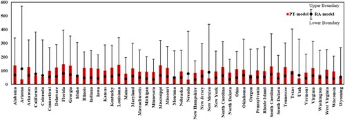
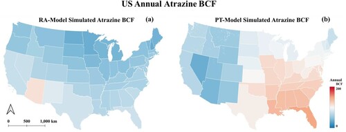
The U.S.A. annual atrazine BCF is 57.69 by RA-model (with an upper boundary value of 576.90 and the lower boundary value of 11.54) and a value of 96.36 by the method proposed in this study. Figure 2 illustrates the annual average atrazine BCF for each state of the U.S.A. simulated through the PT-based model by integrating remote sensing techniques. The black dots in the histogram represent the RA-model simulated annual average atrazine BCF values for the same state with upper and lower boundaries, respectively. If the black dot is within the red bar, the RA-model derived result is lower than the estimated one for the PT-model. Based on Figure 2, the remote sensing derived BCF value is between the upper and lower boundary for all states, indicating that this study’s proposed method integrates PT-model and remote sensing techniques effectively estimate atrazine BCF from the soil in the U.S.A. For forty states (83.33%), the PT-model-derived BCF value is relatively higher than the RA-model-derived one with the black dot within the red bar; the PT-model-derived BCF is lower than the RA-model-derived result for eight states (16.67%). For the RA-model, Arizona has the highest annual average value (113.92), while New Hampshire has the lowest average yearly value (34.28). For the PT-model, Florida has the highest annual average value (146.69), and Nevada has the lowest annual average value (34.51). For most states, the estimated results of the two methods are consistent. In some cases, the RA-model conducted BCF is exceptionally high within the U.S.A., while the PT-model’s effect is relatively underestimated. For instance, Arizona has the highest atrazine BCF value over the U.S.A. using the RA-model, while the PT-model has the second-lowest BCF value (35.6).

Figure 2. The annual Atrazine BCF among the U.S.A. different states.

Figure 3(a) illustrates the distribution of the U.S.A. annual atrazine BCF simulated by the method proposed in this study. The color from blue to red represents the atrazine BCF value ranging from low to high. The eastern part of the U.S.A. has higher BCF values than the western part of the map. Illinois, Indiana, Iowa, and Kansas are states with relatively high atrazine usage, according to the USGS Annual Agricultural Pesticide Use dataset, with the total usage per square mile presented in Table 1. All four states in the region with higher simulated atrazine BCF values have proven that the distribution of atrazine BCF from the soil is relatively consistent with the distribution of the atrazine usage. Figure 3(b) is the scatter plot between RA-model results and the proposed method’s findings. As the scatter plot is distributed along the 1:1 red line, most predictions are concentrated in the upper left region of the red line. The scatter plot demonstrates that the retrieved BCF in this study is consistent with the RA-model, and the retrieved values are relatively higher than the RA-model, consistent with Figure 2. Figure 4(a)–(d) indicates the standard deviation (SD) map and coefficient of variation (CV) map of the RA-model and the PT-model, respectively.

Figure 3. (a) The PT-model simulated U.S.A. annual Atrazine BCF map (b) The relationship between the RA-model and the PT-model derived BCF values.

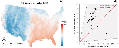
Figure 4. (a) SD map of the RA-model (b) SD map of the PT-model (c) CV map of the RA-model (d) CV map of the PT-model.

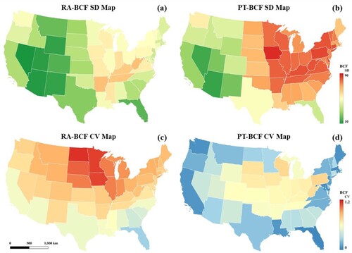
Table 1. Atrazine usage for Illinois, Indiana, Iowa, and Kansas (from the USGS Annual Agricultural Pesticide Use dataset).

State	Total usage (kg)	Usage per square mile
Illinois	4868521.5	84.07
Indiana	2291649.2	62.93
Iowa	305648.5	54.32
Kansas	4062746.1	49.38

Figure 5(a) shows the RA-model simulated state average U.S.A. annual atrazine BCF, while Figure 5(b) shows remote sensing retrieved PT-model based state average U.S.A. annual atrazine BCF. Based on these two figures, although the range of the estimated BCF is similar for both models, the spatial pattern of the state average BCF is quite different for the two models. The higher RA-model estimated BCF values are distributed in the U.S.A. southwest, while the southeast part has relatively higher BCF values through the PT-model. The south region has higher values than the north area of the U.S.A. through the RA-model; however, such a trend only exists in the east of the U.S.A. for the PT-model.

Figure 5. (a) RA-model estimated U.S.A. state average annual Atrazine BCF map (b) PT-model estimated U.S.A. state average annual Atrazine BCF map.

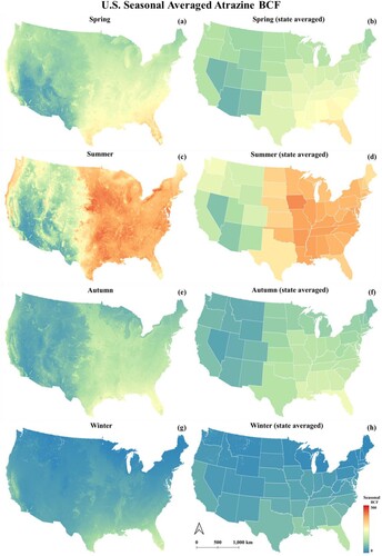
Figure 6 illustrates the state average atrazine BCF value for spring (from March to May), summer (from June to August), autumn (from September to November), and winter (from December to February) estimated using the proposed method in this study. Summer has the highest BCF, with the U.S.A. average atrazine BCF being 164.25; winter has the lowest BCF, with the U.S.A. average atrazine BCF being 26.07; spring has a relatively higher value (the U.S.A. average value equals 94.23) than autumn (the U.S.A. average value is 65.17). The eastern part of the U.S.A. is higher than the west for all seasons, especially in summer. For the east part of the U.S.A., BCF of the south region is lower than that of the north; there is no such pattern over the west part. In winter, Florida has the highest state average atrazine BCF value (43.36), Maine has the lowest average atrazine BCF value (5.22). In spring, Florida has the highest average atrazine BCF value (70.54), whereas Arizona has the lowest average value (41.16); In summer, Iowa has the highest average atrazine BCF value (242.05), with Nevada has the lowest average atrazine BCF value (52.79). In autumn, Florida had the highest average atrazine BCF value (97.34), Nevada had the lowest average atrazine BCF value (28.67). In winter, Florida had the highest average atrazine BCF value (43.27), and Maine had the lowest average atrazine BCF value (5.22).

Figure 6. (a) U.S.A. spring Atrazine BCF map (b) U.S.A. state average spring Atrazine BCF map (c) U.S.A. summer atrazine BCF map (d) U.S.A. state average summer Atrazine BCF map (e) U.S.A. autumn Atrazine BCF map (f) U.S.A. state average autumn Atrazine BCF map (g) U.S.A. winter Atrazine BCF map (h) U.S.A. state average winter Atrazine BCF map.

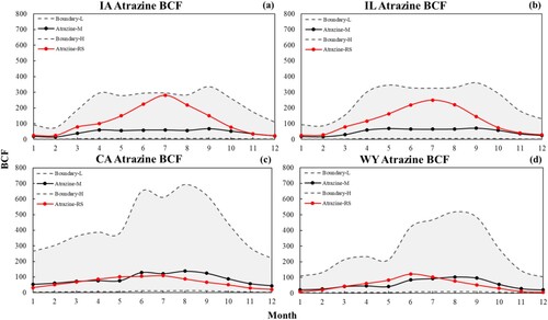
Figure 7(a)–(d) shows the time series of average atrazine BCF for Iowa, Illinois, California, and Wyoming, respectively. Iowa and Illinois are agricultural states with high atrazine usage, while California and Wyoming are agricultural states with limited atrazine application. In the time series, the red line refers to the PT-model-derived BCF, the black line refers to the RA-model-derived BCF, and the grey dashed line refers to the upper and lower boundary of the RA-model. The red line is within the light grey area, indicating that the estimated atrazine using this study’s proposed method is within the considerable range. The red line is within the grey area for all four states from the time series. For California and Wyoming, the red line is relatively consistent with the black line, which means the proposed method has the same temporal distribution as the RA-model for states with limited usage of atrazine. For Illinois and Iowa, both models have relatively higher values in summer than in winter, spring, and fall. Still, the PT-model simulated BCF is exceptionally high in June, July, and August, which is inconsistent with the RA-model results temporal distribution.

Figure 7. (a) Iowa annual time series of Atrazine BCF (b) Illinois annual time series of Atrazine BCF (c) California annual time series of Atrazine BCF (d) Wyoming annual time series of Atrazine BCF.

4. Discussion

Plant uptake of pesticides from soil modeling is still a challenging task to fulfill, especially monitoring its spatiotemporal distribution. Mapping the spatiotemporal patterns of pesticide bioconcentration from the soil is significant to environmental protection, food security, health risk assessment, and land planning. BCF is applied to indicate the potential of pesticide bioconcentration from the soil, and pesticide bioconcentration can then be estimated, mainly integrating the usage of pesticides and the degradation of pesticides in the soil. This study employed a simplified plant uptake model combined with remote sensing techniques to map the spatiotemporal patterns of pesticides BCF from the soil. However, several issues remained.

First, the RA-model applied for evaluation has limitations: (1) The monthly or seasonal average air temperature and relative humidity datasets obtained from meteorological stations were used in the verified RA-model to predict the spatiotemporal patterns of pesticides BCF. The state average value may not have a good representative due to the spare distribution of the stations (Sun et al. 2005). Remote sensing is also an effective tool to monitor spatiotemporal continuous air temperature and relative humidity, which many previous studies have proposed and explored (Dehennis and Wise 2005; Sun et al. 2005). Further studies will be focused on integrating remote sensing techniques and RA-model for pesticide BCF mapping. (2) Canopy condition is represented by the leaf area index (LAI) and assumed to be stable in the RA-model; however, the global vegetation state varies significantly throughout the year. Although the variation of air temperature and humidity may partially represent the distribution of vegetation conditions, the lack of spatiotemporal continuous LAI observation may introduce uncertainty to the estimations. Remote sensing can be applied to estimate LAI at good resolutions with high accuracy to improve the prediction performance (Zheng and Moskal 2009).

Second, the one-component method proposed in this study mainly considers the leaf uptake of pesticides from soil. Other parts of the plant, such as fruit and stem, may also uptake pesticides from the soil. The fruit, stems, and other plant parts, which favor the uptake of pesticides, must be considered (Kumari and John 2019; Pico et al. 2018). Multi-compartment model assimilated environment conditions will be developed to improve the accuracy of plant pesticide uptake simulation.

Third, various environment-related factors, such as wind speed and precipitation, are critical indicators of the plant uptake of organic matter from the soil, which was not involved in the proposed method. Besides, the spatiotemporal distribution of the pesticide dosage is another crucial factor that may affect the pesticide uptake from the soil for specific types (Yao et al. 2006). The spatial pattern of atrazine usage is relatively consistent with PT-model simulated atrazine BCF from the soil. Still, the pesticide dosage has not been considered in the PT-model or RA-model. Therefore, more spatiotemporal distributed significant variables should be assimilated further to improve the model’s accuracy. Moreover, we only used atrazine as an example in this study due to its wide application in the U.S.A. The spatiotemporal patterns of similar pesticides should be simulated through the proposed method to evaluate the further application of the plant transpiration-based model integrating remote sensing techniques.

Fourth, remote sensing techniques and retrieval procedures introduce uncertainties: (1) Satellite sensors generally contain spectral noises, and the surface reflectance observations applied in this study may be affected by weather conditions (Xu et al. 2020). (2) The vegetation index (EVI) was applied in this study to estimate plant transpiration based on the theory that EVI varies with vegetation coverage and type (e.g. conifer and broadleaf), which are highly related to plant transpiration (Li et al. 2010; Yan et al. 2015). Consequently, the BCF’s spatial pattern may depend on the vegetation type as well. The spatial resolution of remote sensing products applied in this study is 500 m, so there may be a mixture of various vegetation types within the pixel. Estimating the ratio between different vegetation types within the pixel may improve plant transpiration and BCF mapping, which will be focused on in future work.

Fifth, ground truth observations for the plant uptake of atrazine from the soil are lacking due to time restraints and resource unavailability, which is the study’s motivation to integrate a theoretical model with remote sensing to estimate BCF. Nevertheless, the lack of field data makes it difficult to calibrate and validate the proposed model. Although the RA-model and PT-model are generally consistent, the spatial distribution is different, and such a preliminary result needs to be verified and analyzed by field observations.

5. Conclusion

In this study, a simplified one-compartment plant uptake model (PT-model) was developed to monitor pesticide BCF from soil based on its correlation between plant transpiration. Spatiotemporal continuous pesticides’ BCF was retrieved by integrating the proposed PT-model and remote sensing observations, and atrazine’s BCF over the U.S.A was mapped consequently. This research highlights that plant transpiration plays a vital role in BCF monitoring; BCF’s spatial distribution varies with time. For the mainland of the U.S.A., summer has the highest BCF value, and winter has the lowest BCF value; BCF of the east part is relatively higher than the west all over the year. Previous studies with relatively good consistency have been applied to evaluate the proposed approach.

To further understand the spatiotemporal distribution of pesticide BCF, future research is needed in the following aspects:

1. Downscaling methods and high-resolution remote sensing observations will be integrated to classify different vegetation types, especially over the agricultural area. Then the plant transpiration over specific vegetation cover will be estimated separately to improve and calibrate the PT-model’s performance for BCF monitoring. Since plant transpiration relates to species (e.g. conifer, broadleaf), the monitored spatiotemporal patterns of BCF also depend on the vegetation type.

2. Atrazine is applied in this study because it is one of the most widely used pesticides in the U.S.A in recent decades, which is difficult to degrade and has significant residues. The PT-model will be applied to other pesticides with harmful residues to the environment and human health (e.g. hexachlorocyclohexane, lindane) to evaluate the PT-model’s performance in BCF mapping. Besides that, experiments and field campaigns will be carried out to collect in-situ measurements to validate the results of the PT-model.

3. Various studies show that pesticide BCF potentially affects human health. However, few studies analyze the relationship between pesticide BCF distribution and human disease distribution (e.g. cancer and congenital heart disease) due to the lack of large-scale BCF mapping methods. We plan to combine open-source human disease datasets in the U.S.A. and pesticide BCF spatiotemporal distributions to explore the potential impacts of pesticide BCF on different human diseases.

Acknowledgements

We thank the editors and reviewers for their valuable comments to improve this manuscript.

Disclosure statement

No potential conflict of interest was reported by the author(s).

Data availability

The data that support the findings of this study are openly available in NASA MODIS Portal (https://modis.gsfc.nasa.gov/), USGS Annual Agricultural Pesticide Use dataset (https://water.usgs.gov/nawqa/pnsp/usage/maps/compound_listing.php), Fantke et al. (2017) and Lewis et al. (2006).

Additional information

Funding

This research was supported by the Natural Resources of Guangdong [No. [2023]-25], National Natural Science Foundation of China [No. 42171400], Natural Science Foundation of Guangdong Province [No. 2021A1515011324], Henan Institute of Sun Yat-sen University [No. 2021-006].

References

- Akter, M., L. Fan, M. M. Rahman, V. Geissen, and C. J. Ritsema. 2018. “Vegetable Farmers’ Behaviour and Knowledge Related to Pesticide use and Related Health Problems: A Case Study from Bangladesh.” Journal of Cleaner Production 200: 122–133. doi:10.1016/j.jclepro.2018.07.130.
- Alamdar, A., J. H. Syed, R. N. Malik, A. Katsoyiannis, J. Liu, J. Li, G. Zhang, and K. C. Jones. 2014. “Organochlorine Pesticides in Surface Soils from Obsolete Pesticide Dumping Ground in Hyderabad City, Pakistan: Contamination Levels and Their Potential for Air–Soil Exchange.” Science of the Total Environment 470: 733–741. doi:10.1016/j.scitotenv.2013.09.053.
- Bhandari, G., K. Atreya, P. T. Scheepers, and V. Geissen. 2020. “Concentration and Distribution of Pesticide Residues in Soil: Non-Dietary Human Health Risk Assessment.” Chemosphere 253: 126594. doi:10.1016/j.chemosphere.2020.126594.
- Bhattarai, N., and P. Wagle. 2021. “Recent Advances in Remote Sensing of Evapotranspiration.” Remote Sensing 13 (21): 4260. doi:10.3390/rs13214260.
- Briggs, G. G., R. H. Bromilow, and A. A. Evans. 1982. “Relationships Between Lipophilicity and Root Uptake and Translocation of Non-Ionised Chemicals by Barley.” Pesticide Science 13 (5): 495–504. doi:10.1002/ps.2780130506.
- Calderbank, A. 1989. “The Occurrence and Significance of Bound Pesticide Residues in Soil.” In Reviews of Environmental Contamination and Toxicology, edited by George W. Ware, 71–103. New York: Springer Verlag.
- Collins, C. D., and E. Finnegan. 2010. “Modeling the Plant Uptake of Organic Chemicals, Including the Soil–Air–Plant Pathway.” Environmental Science & Technology 44 (3): 998–1003. doi:10.1021/es901941z.
- de Albuquerque, F. P., J. L. de Oliveira, V. Moschini-Carlos, and L. F. Fraceto. 2020. “An Overview of the Potential Impacts of Atrazine in Aquatic Environments: Perspectives for Tailored Solutions Based on Nanotechnology.” Science of the Total Environment 700: 134868. doi:10.1016/j.scitotenv.2019.134868.
- Dehennis, A. D., and K. D. Wise. 2005. “A Wireless Microsystem for the Remote Sensing of Pressure, Temperature, and Relative Humidity.” Journal of Microelectromechanical Systems 14 (1): 12–22. doi:10.1109/JMEMS.2004.839650.
- Doucette, W. J., C. Shunthirasingham, E. M. Dettenmaier, R. T. Zaleski, P. Fantke, and J. A. Arnot. 2018. “A Review of Measured Bioaccumulation Data on Terrestrial Plants for Organic Chemicals: Metrics, Variability, and the Need for Standardized Measurement Protocols.” Environmental Toxicology and Chemistry 37 (1): 21–33. doi:10.1002/etc.3992.
- Fantke, P., M. Bijster, C. Guignard, M. Z. Hauschild, M. Huijbregts, O. Jolliet, A. Kounina, et al. 2017. USEtox® 2.0 Documentation (Version 1.00).
- Fantke, P., R. Charles, L. F. de Alencastro, R. Friedrich, and O. Jolliet. 2011. “Plant Uptake of Pesticides and Human Health: Dynamic Modeling of Residues in Wheat and Ingestion Intake.” Chemosphere 85 (10): 1639–1647. doi:10.1016/j.chemosphere.2011.08.030.
- Fatnassi, H., T. Boulard, and J. Lagier. 2004. “Simple Indirect Estimation of Ventilation and Crop Transpiration Rates in a Greenhouse.” Biosystems Engineering 88 (4): 467–478. doi:10.1016/j.biosystemseng.2004.05.003.
- Hsu, F. C., R. L. Marxmiller, and A. Y. Yang. 1990. “Study of root uptake and xylem translocation of cinmethylin and related compounds in detopped soybean roots using a pressure chamber technique.” Plant Physiology 93 (4): 1573–1578. doi:10.1104/pp.93.4.1573.
- Hwang, J. I., S. E. Lee, and J. E. Kim. 2017. “Comparison of Theoretical and Experimental Values for Plant Uptake of Pesticide from Soil.” PLoS One 12 (2): e0172254. doi:10.1371/journal.pone.0172254.
- Hwang, J. I., A. R. Zimmerman, and J. E. Kim. 2018. “Bioconcentration Factor-Based Management of Soil Pesticide Residues: Endosulfan Uptake by Carrot and Potato Plants.” Science of the Total Environment 627: 514–522. doi:10.1016/j.scitotenv.2018.01.208.
- Islam, M. N., L. Huang, and S. D. Siciliano. 2020. “Inclusion of Molecular Descriptors in Predictive Models Improves Pesticide Soil-air Partitioning Estimates.” Chemosphere 248: 126031. doi:10.1016/j.chemosphere.2020.126031.
- Juraske, R., F. Castells, A. Vijay, P. Muñoz, and A. Antón. 2009. “Uptake and Persistence of Pesticides in Plants: Measurements and Model Estimates for Imidacloprid After Foliar and Soil Application.” Journal of Hazardous Materials 165 (1-3): 683–689. doi:10.1016/j.jhazmat.2008.10.043.
- Köhne, J. M., S. Köhne, and J. Šimůnek. 2009. “A Review of Model Applications for Structured Soils: B) Pesticide Transport.” Journal of Contaminant Hydrology 104 (1-4): 36–60. doi:10.1016/j.jconhyd.2008.10.003.
- Kool, D., N. Agam, N. Lazarovitch, J. L. Heitman, T. J. Sauer, and A. Ben-Gal. 2014. “A Review of Approaches for Evapotranspiration Partitioning.” Agricultural and Forest Meteorology 184: 56–70. doi:10.1016/j.agrformet.2013.09.003.
- Kumari, D., and S. John. 2019. “Health Risk Assessment of Pesticide Residues in Fruits and Vegetables from Farms and Markets of Western Indian Himalayan Region.” Chemosphere 224: 162–167. doi:10.1016/j.chemosphere.2019.02.091.
- Lewis, K., J. Tzilivakis, A. Green, and D. Warner. 2006. Pesticide Properties DataBase (PPDB).
- Li, Z. 2020. “Spatiotemporal Pattern Models for Bioaccumulation of Pesticides in Common Herbaceous and Woody Plants.” Journal of Environmental Management 276: 111334. doi:10.1016/j.jenvman.2020.111334.
- Li, Z., and Z. Ai. 2023. “Mapping Plant Bioaccumulation Potentials of Pesticides from Soil Using Satellite-Based Canopy Transpiration Rates.” Environmental Toxicology and Chemistry 42 (1): 117–129. doi:10.1002/etc.5511.
- Li, X., P. Gentine, C. Lin, S. Zhou, Z. Sun, Y. Zheng, J. Liu, and C. Zheng. 2019. “A Simple and Objective Method to Partition Evapotranspiration Into Transpiration and Evaporation at Eddy-Covariance Sites.” Agricultural and Forest Meteorology 265: 171–182. doi:10.1016/j.agrformet.2018.11.017.
- Li, Z., X. Li, D. Wei, X. Xu, and H. Wang. 2010. “An Assessment of Correlation on MODIS-NDVI and EVI with Natural Vegetation Coverage in Northern Hebei Province, China.” Procedia Environmental Sciences 2: 964–969. doi:10.1016/j.proenv.2010.10.108.
- Miao, J., X. Chen, T. Xu, D. Yin, X. Hu, and G. D. Sheng. 2018. “Bioaccumulation, Distribution and Elimination of Lindane in Eisenia Foetida: The Aging Effect.” Chemosphere 190: 350–357. doi:10.1016/j.chemosphere.2017.09.138.
- Mu, Q., F. A. Heinsch, M. Zhao, and S. W. Running. 2007. “Development of a Global Evapotranspiration Algorithm Based on MODIS and Global Meteorology Data.” Remote Sensing of Environment 111 (4): 519–536. doi:10.1016/j.rse.2007.04.015.
- Mu, Q., M. Zhao, and S. W. Running. 2011. “Improvements to a MODIS Global Terrestrial Evapotranspiration Algorithm.” Remote Sensing of Environment 115 (8): 1781–1800. doi:10.1016/j.rse.2011.02.019.
- Neale, P.A., S. Ait-Aissa, W. Brack, N. Creusot, M.S. Denison, B. Deutschmann, K. Hilscherová, et al. 2015. “Linking in vitro effects and detected organic micropollutants in surface water using mixture-toxicity modeling.” Environmental science & technology 49 (24): 14614–14624. doi:10.1021/acs.est.5b04083.
- Niu, Z., H. He, G. Zhu, X. Ren, L. Zhang, and K. Zhang. 2020. “A Spatial-Temporal Continuous Dataset of the Transpiration to Evapotranspiration Ratio in China from 1981–2015.” Scientific Data 7 (1): 1–13. doi:10.1038/s41597-019-0340-y.
- Philippe, V., A. Neveen, A. Marwa, and A. Y. A. Basel. 2021. “Occurrence of Pesticide Residues in Fruits and Vegetables for the Eastern Mediterranean Region and Potential Impact on Public Health.” Food Control 119: 107457. doi:10.1016/j.foodcont.2020.107457.
- Pico, Y., M. A. El-Sheikh, A. H. Alfarhan, and D. Barcelo. 2018. “Target vs Non-Target Analysis to Determine Pesticide Residues in Fruits from Saudi Arabia and Influence in Potential Risk Associated with Exposure.” Food and Chemical Toxicology 111: 53–63. doi:10.1016/j.fct.2017.10.060.
- Rein, A., C. N. Legind, and S. Trapp. 2011. “New concepts for dynamic plant uptake models.” SAR and QSAR in Environmental Research 22 (1-2): 191–215. doi:10.1080/1062936X.2010.548829.
- Sanchez, S. A. V., A. Mentler, M. Gartner, A. Gschaider, J. van der Poel, R. M. Kral, A. Ngadisih, and K. M. Keiblinger. 2019. “Pesticide Residues in Intensive Agricultural Soils are Higher Than in Agroforestry Systems – A Case Study on the Indonesian Dieng Plateau.” Geophysical Research Abstracts 21.
- Silva, V., H. G. Mol, P. Zomer, M. Tienstra, C. J. Ritsema, and V. Geissen. 2019. “Pesticide Residues in European Agricultural Soils – A Hidden Reality Unfolded.” Science of the Total Environment 653: 1532–1545. doi:10.1016/j.scitotenv.2018.10.441.
- Singh, S., V. Kumar, A. Chauhan, S. Datta, A. B. Wani, N. Singh, and J. Singh. 2018. “Toxicity, Degradation and Analysis of the Herbicide Atrazine.” Environmental Chemistry Letters 16 (1): 211–237. doi:10.1007/s10311-017-0665-8.
- Sun, S., V. Sidhu, Y. Rong, and Y. Zheng. 2018. “Pesticide Pollution in Agricultural Soils and Sustainable Remediation Methods: A Review.” Current Pollution Reports 4 (3): 240–250. doi:10.1007/s40726-018-0092-x.
- Sun, Y. J., J. F. Wang, R. H. Zhang, R. R. Gillies, Y. Y. C. B. Xue, and Y. C. Bo. 2005. “Air Temperature Retrieval from Remote Sensing Data Based on Thermodynamics.” Theoretical and Applied Climatology 80: 37–48. doi:10.1007/s00704-004-0079-y.
- Trapp, S. 2003. “Harmonized European Assssment for the Transfer of Chemicals from Soil into Food.” Journal of Soils and Sediments 3 (1): 6. doi:10.1007/BF02989461.
- Trapp, S., A. Cammarano, E. Capri, F. Reichenberg, and P. Mayer. 2007. “Diffusion of PAH in Potato and Carrot Slices and Application for a Potato Model.” Environmental Science & Technology 41 (9): 3103–3108. doi:10.1021/es062418o.
- Trapp, S., and M. Matthies. 1995. “Generic One-Compartment Model for Uptake of Organic Chemicals by Foliar Vegetation.” Environmental Science & Technology 29 (9): 2333–2338. doi:10.1021/es00009a027.
- Tudi, M., H. Daniel Ruan, L. Wang, J. Lyu, R. Sadler, D. Connell, C. Chu, and D. T. Phung. 2021. “Agriculture Development, Pesticide Application and its Impact on the Environment.” International Journal of Environmental Research and Public Health 18 (3): 1112. doi:10.3390/ijerph18031112.
- Tulcan, R. X. S., W. Ouyang, X. Gu, C. Lin, M. Tysklind, and B. Wang. 2021. “Typical Herbicide Residues, Trophic Transfer, Bioconcentration, and Health Risk of Marine Organisms.” Environment International 152: 106500. doi:10.1016/j.envint.2021.106500.
- Velpuri, N. M., G. B. Senay, R. K. Singh, S. Bohms, and J. P. Verdin. 2013. “A Comprehensive Evaluation of two MODIS Evapotranspiration Products Over the Conterminous United States: Using Point and Gridded FLUXNET and Water Balance ET.” Remote Sensing of Environment 139: 35–49. doi:10.1016/j.rse.2013.07.013.
- Xiao, S., Z. Li, and P. Fantke. 2021. “Improved Plant Bioconcentration Modeling of Pesticides: The Role of Periderm Dynamics.” Pest Management Science 77 (11): 5096–5108. doi:10.1002/ps.6549.
- Xu, T., S. M. Bateni, S. A. Margulis, L. Song, S. Liu, and Z. Xu. 2016. “Partitioning Evapotranspiration into Soil Evaporation and Canopy Transpiration via a two-Source Variational Data Assimilation System.” Journal of Hydrometeorology 17 (9): 2353–2370. doi:10.1175/JHM-D-15-0178.1.
- Xu, C., J. J. Qu, X. Hao, Z. Zhu, and L. Gutenberg. 2020. “Monitoring Soil Carbon Flux with in-Situ Measurements and Satellite Observations in a Forested Region.” Geoderma 378: 114617. doi:10.1016/j.geoderma.2020.114617.
- Xu, X., R. Zarecki, S. Medina, S. Ofaim, X. Liu, C. Chen, S. Hu, et al. 2019. “Modeling Microbial Communities from Atrazine Contaminated Soils Promotes the Development of Biostimulation Solutions.” The ISME Journal 13 (2): 494–508. doi:10.1038/s41396-018-0288-5.
- Yan, E., G. Wang, H. Lin, C. Xia, and H. Sun. 2015. “Phenology-Based Classification of Vegetation Cover Types in Northeast China Using MODIS NDVI and EVI Time Series.” International Journal of Remote Sensing 36 (2): 489–512. doi:10.1080/01431161.2014.999167.
- Yao, Y., L. Tuduri, T. Harner, P. Blanchard, D. Waite, L. Poissant, C. Murphy, et al. 2006. “Spatial and Temporal Distribution of Pesticide Air Concentrations in Canadian Agricultural Regions.” Atmospheric Environment 40 (23): 4339–4351. doi:10.1016/j.atmosenv.2006.03.039.
- Yu, X. Y., G. G. Ying, and R. S. Kookana. 2009. “Reduced Plant Uptake of Pesticides with Biochar Additions to Soil.” Chemosphere 76 (5): 665–671. doi:10.1016/j.chemosphere.2009.04.001.
- Zhang, W. 2018. “Global Pesticide Use: Profile, Trend, Cost/Benefit and More.” Proceedings of the International Academy of Ecology and Environmental Sciences 8 (1): 1–27.
- Zhang, K., J. S. Kimball, and S. W. Running. 2016. “A Review of Remote Sensing Based Actual Evapotranspiration Estimation.” WIRES Water 3 (6): 834–853. doi:10.1002/wat2.1168.
- Zheng, G., and L. M. Moskal. 2009. “Retrieving Leaf Area Index (LAI) Using Remote Sensing: Theories, Methods and Sensors.” Sensors 9 (4): 2719–2745. doi:10.3390/s90402719.