Retrieving the grounding lines of the Riiser-Larsen Ice Shelf using Sentinel-1 SAR images

ABSTRACT

Accurately locating and studying grounding lines is essential for predicting the response of glaciers to climate change. However, it is challenging to find grounding lines since they are subglacial features. In this study, Sentinel-1 synthetic aperture radar (SAR) data were utilized to derive the grounding lines of the Riiser-Larsen Ice Shelf. A new method with inspiration drawn from multi-temporal baseline InSAR techniques is proposed. It takes advantage of the temporal consistency of the vertical displacement gradients and identifies grounding zones pixel-by-pixel on a stack of double differential interferograms, thereby providing grounding line proxies. As it fully exploits coherent signals in both spatial and temporal domains, the maximum possible number of grounding zone pixels can be obtained. Moreover, due to the introduction of the concept of the temporal consistency, the method can cope with short term grounding line fluctuations to some extent and may mitigate the influences of atmospheric disturbances and residual ice displacements. The resulting grounding lines are compared with the MEaSUREs Antarctic grounding line product. The comparison confirms the effectiveness of the proposed method and corroborates that the Riiser-Larsen Ice Shelf should have not undergone significant changes over the past few decades.

KEYWORDS:

• Antarctica
• ice shelf
• grounding line
• radar interferometry
• Sentinel-1 images

1. Introduction

Grounding lines serve as a fundamental indicator of the stability of an ice shelf (Rack et al. 2017), marking the boundaries between the grounded ice of an ice sheet or tidewater glacier and the floating ice of an ice shelf or glacier tongue. They are defined by the position at which grounded ice separates from the glacier bedrock and begins to flow into the ocean, signifying the transition from fully grounded ice to freely floating ice (Friedl et al. 2020). The flow dynamics of grounded ice are primarily governed by shear and basal resistance, while floating ice exhibits no resistance and is primarily controlled by membrane stress (Rignot, Mouginot, and Scheuchl 2011). The location of grounding lines is therefore critical in understanding different flow mechanisms, and serves as a crucial boundary condition for studying the physical status of glaciers, global climate change and sea level change.

It is worth noting that the location of a grounding line may vary in space and time due to several factors, such as changes in ice thickness (Zhao et al. 2022) or sea level (Adhikari et al. 2014). Consequently, accurately identifying grounding lines can be a challenging task. While several field techniques have been successfully used to detect grounding lines (Le Meur et al. 2014; Rosenau et al. 2013), they are limited by logistical difficulties, sparse coverage and the high cost of repeatedly gathering data (Hogg et al. 2016).

Remote sensing methods have been increasingly applied for mapping grounding lines (Kim and Kim 2017; Rebesco et al. 2014; Rignot et al. 2014). These methods can generally be classified into three categories (Friedl et al. 2020): hydrostatic, ice slope and tidal methods. Hydrostatic methods are used to extract the lines of the first hydrostatic equilibrium, which can be considered as a proxy for the true grounding lines (Fricker et al. 2002). Friedl et al. (2018) applied this method to calculate the hydrostatic equilibrium and derive the change in the grounding line of the Fleming Glacier, revealing that it (the grounding line) substantially retreated. However, the accuracy of this method is highly dependent on several locally varying factors, such as ice thickness, ice density and firn depth correction (Griggs and Bamber 2011). Ice slope methods primarily use optical or radar altimeter data to identify grounding lines. As the basal ice abruptly separates from the ground to the ocean, the ice becomes thinner along the ice flow direction, leading to a slope break in the ice surface (Schoof 2007). Grounding lines can, therefore, be identified based on the position of the surface slope break (Herzfeld et al. 2008), which can be obtained based on the elevation data from radar altimetry (Yang et al. 2022). Herzfeld et al. (2008) utilized ICESat geoscience laser altimeter system (GLAS) data and ERS-1 radar altimeter data to analyze the grounding line change of the Pine Island Glacier, while Dawson and Bamber (2020) used CryoSat-2 data to map grounding lines across Antarctica. Note that optical images can also be used to identify surface slope breaks by identifying topographic shadows. Since optical images are widely available over Antarctica, this method is used to map complete grounding lines throughout the continent (Bindschadler et al. 2011). However, it might produce grounding lines with relatively large deviations in fast-flow areas, since ice dynamics may change gradually on the surface (Rignot, Mouginot, and Scheuchl 2011).

The idea of tidal methods is to extract grounding lines by analyzing the ice vertical displacements induced by tides. Synthetic aperture radar interferometry (InSAR) is currently the most promising remote sensing technique for measuring ground surface deformation (Goldstein et al. 1993; Joughin, Smith, and Abdalati 2010). This technique uses two synthetic aperture radar (SAR) images taken at different times and locations to generate an interferogram. Based on the phase information in the interferogram, deformation products with a precision of centimeters can be obtained (Zebker 2017). Due to its high precision, InSAR has been introduced to detect grounding lines. It is worth noting that InSAR measurements are a projection of both horizontal and vertical deformation in the radar line-of-sight (LOS) direction. However, the vertical deformation induced by tides cannot be readily obtained by InSAR, which makes it difficult to directly identify grounding lines (Rack et al. 2017). Rignot (1996) proposed the so-called double differential radar interferometry to solve this problem. This method generates a double differential interferogram by subtracting the phase of two interferograms, assuming that the horizontal deformation phase in the two interferograms is equal. In this case, it can be considered that the double differential interferogram only contains the phase related to the vertical deformation (Han and Lee 2014). As the vertical deformation is caused by tides, the double differential interferometric phases over grounding zones will show dense fringes (Lee et al. 2021). The location where obvious interferometric fringes first appear in the direction from grounded ice to floating ice is considered to be the grounding line proxy (Rignot, Mouginot, and Scheuchl 2011). Double differential radar interferometry delineates the inland limit of tidal flexure, which is referred to as grounding line throughout this paper. In recent years, double differential radar interferometry has increasingly been utilized in grounding line mapping applications. Floricioiu et al. (2012) successfully analyzed TerraSAR-X acquisitions to obtain grounding lines over Byrd, Nimrod and Beardmore glaciers. Han and Lee (2014) applied this technique to one-day tandem interferometric SAR images from COSMO-SkyMed over the Campbell Glacier Tongue, demonstrating that the grounding lines of the tongue retreated from 1996 to 2010. Scheuchl et al. (2016) generated grounding line maps for Pope, Smith and Kohler glaciers in West Antarctica using Sentinel-1A data spanning the period from 2014 to 2016. Milillo et al. (2017) investigated the migration of the Pine Island Glacier grounding lines using COSMO-SkyMed data. However, the double differential radar interferometry mainly faces three problems. First, the position where the fringes appear is currently mainly delineated manually, which is time-consuming and may lead to deviations. Second, the interferometric signal in polar regions is easily affected by temporal decorrelation due to two reasons. (1) The ice melting changes the backscattering characteristics of glacier surface; (2) Fast ice flow will introduce large deformation signals, causing the frequency of interferometric fringes to exceed the sampling frequency of a double differential interferogram (In this study, this phenomenon is referred to as phase saturation Zhang et al. 2010). Therefore, in a single double differential interferogram, interferometric coherence may not be preserved in localized grounding zones. Consequently, it is hard to preserve the integrity of grounding line results. Third, in practical applications, it is difficult to ensure that the horizontal deformation phase in the two interferograms is exactly the same. The presence of residual horizontal deformation will exert negative impacts on the accuracy of grounding line identification.

This study aims to extract the grounding lines over the Riiser-Larsen Ice Shelf using Sentinel-1 SAR data. The Riiser-Larsen Ice Shelf is a floating ice mass situated on the coast of Queen Maud Land in Antarctica. Its length is approximately 400 km (Moussavi et al. 2020), and its area is approximately 48,180 square kilometers (Dirscherl, Dietz, and Kuenzer 2021). The ice discharge from the Riiser-Larsen Ice Shelf is a significant water mass contributor to the eastern Weddell Sea (Thoma, Grosfeld, and Lange 2006). The ice shelf has been the subject of extensive scientific researches (Hillenbrand et al. 2014; Rignot et al. 2019), particularly in relation to climate change and its potential impacts on sea level rise.

Inspired by multi-temporal baseline InSAR techniques (Berardino et al. 2002; Ferretti, Prati, and Rocca 2001), a new method that works based on a stack of double differential interferograms, rather than a single one, is developed. It identifies grounding zones by taking advantage of the temporal homogeneousness of the direction of the vertical displacement gradients, thereby generating grounding line proxies. The main advantages of this method can be summarized as follows: (1) The method identifies grounding zones on a pixel-by-pixel basis, which circumvents manual manipulations effectively; (2) The method fully mines coherent signals contained in all double differential interferograms, ensuring as many grounding zones as possible are extracted; (3) The method may mitigate the impacts of residual horizontal motion and atmospheric disturbances, and is generally able to deal with the problem of short term grounding line fluctuations, as the estimation of the direction homogeneousness can be considered to be a temporal averaging process.

2. Study area and input data

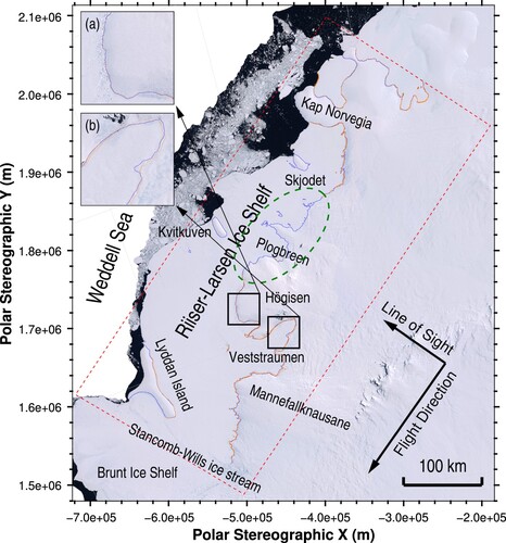
The Riiser-Larsen Ice Shelf is located on the western edge of Dronning Maud Land and the eastern region of Oates Land in Antarctica. As shown in Figure 1, it stretches from Cape Norvegia in the north to Lyddan Island and the Stancomb-Wills Glacier in the south. There are three ice rises near the calving front, namely Lyddan Island, Kvitkuven and Skjoldet, which act as buttressing points within the ice shelf and ensure the stability of the ice shelf to some extent (Favier et al. 2016). The ice shelf is primarily fed by the Veststraumen and Plogbreen ice streams, which are separated by the dome-shaped Högisen.

Figure 1. The location of the Riiser-Larsen Ice Shelf. The background optical image is provided by the Landsat Image Mosaic of Antarctica (LIMA) (Bindschadler et al. 2008). The red dashed rectangle indicates the coverage of the cropped data.

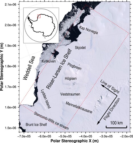
Overall, sixty European Space Agency's Sentinel-1B single look complex (SLC) images, which are available at the Copernicus open access hub, were utilized in this study. These images were acquired between January 5, 2020 and December 23, 2021, in interferometric wide (IW) swath mode, with an incidence angle ranging from 29 to 44 degrees. The images are from Path 50, Frame 836–856. Their spatial resolutions in azimuth and range directions are approximately 20 m and 5 m, respectively. To fit the coverage of the Riiser-Larsen Ice Shelf more precisely, each SLC was slightly cropped. The coverage of the cropped data is indicated by the red dashed rectangle in Figure 1. The SAR sensor's flight and look directions are indicated by the two black arrows, respectively. The data are in the horizontal transmit and horizontal receive (HH) polarization, which is particularly suitable for glacier applications as it offers better amplitude characteristics and a higher signal-to-noise ratio (SNR) (Sánchez-Gámez and Navarro 2017).

3. Methodology

3.1. Data preprocessing

The proposed method utilizes a stack of double differential interferograms to identify grounding zones by analyzing the interferometric signals' characteristics in the temporal dimension. It requires the projection of all images taken at different orbital positions onto a same grid. As indicated in Figure 1, the heading angle (the angle between the flight path and the Y direction) is approximately ${145}^{\circ }$. It implies that the required storage of the data in polar stereographic coordinate is approximately twofold of that of the data in the radar coordinate. In order to carry out the proposed method in the radar coordinate, a common master image is required to be selected as the reference. Moreover, the minimum temporal baseline of the input data is 12 days. Due to the ice movements, large and super-nonlinear offsets will be present between any two SAR images in ice shelf areas. The commonly used enhanced spectral diversity (ESD) (Yagüe-Martínez et al. 2016) based coregistration approach for Sentinel-1 IW data is not competent to generate coherent interferometric signals over the ice shelf areas.

Figure 2 demonstrates the processing steps adopted to retrieve interferometric signals. Below is a sequential listing of the description for each step. Note that except for the interpolation process, all basic interferometric processing steps were implemented by the authors using C++.

Figure 2. The flowchart of the data preprocessing.

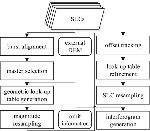
(1)	Burst alignment: As the Sentinel-1B sensor operated in IW mode over the study area, the burst data with respect to each acquisition are firstly aligned to an image with successive observations analogous to stripe mode data by using the clock information in azimuth and range directions.
(2)	Master selection and look-up table generation: For simplicity, the SAR image taken on December 6, 2020 is chosen as the master as it is located in the middle of the observation cycle. Next, a look-up table with respect to the aligned master grid, which depicts the correspondence of pixel positions between two images, is created for each slave image using orbit information and the external digital elevation model (DEM) provided by the Reference Elevation Model of Antarctica (REMA) (Howat et al. 2019). The Copernicus Sentinel-1 precise orbit product is incorporated into this process. Its accuracy typically falls below 1 cm (Yagüe-Martínez et al. 2016), which effectively compensates for any geometrical distortion due to the various satellite observation positions (e.g. Zebker 2017 has generated interferograms in geographic coordinates directly from the precise orbit data.)
(3)	Magnitude resampling and offset tracking: Based on the look-up tables, all aligned slave images are resampled to the master's grid using an $8\times 8$ sinc kernel. It is important to note that the resampling is performed directly on the magnitude of SAR images. Therefore, there is no need for a deramping (the removal of the phase ramp caused by the movement of the radar platform during the acquisition of the radar data) (Yagüe-Martínez et al. 2016) operation. In this study, we utilize temporally adjacent SAR images to generate interferometric signals, which forms 59 interferometric pairs with a temporal baseline of 12 days. Subsequently, we apply offset tracking between the resampled images with respect to each pair, with a window size of $32\times 128$. For the purpose of balancing spatial resolutions in azimuth and range directions, the intervals between nearby windows are irregularly assigned ($10\times 40$ pixels). Unreliable offset tracking observations are removed based on the SNRs of the corresponding convolutions. The open-source software Surfit (Mikhail and Vladimir 2021), which incorporates the consecutive minimization of functional sequence method, is used to interpolate the offset map.
(4)	Look-up table refinement and SLC resampling: For clarity, the terms SLC1 and SLC2 are used to refer to the two images in a given pair. It is important to note that the 12-day interval between acquisitions can cause additional distortions in SLC2 relative to SLC1 due to the ice movement. As the offset map directly depicts such distortions, a new look-up table for SLC2 is generated by compensating the original look-up table pixel by pixel with the use of the offset map. Next, the bursts of SLC1 are resampled using the original look-up table, while the bursts of SLC2 are resampled using the compensated look-up table. Subsequently, the resampled bursts of each image are aligned using the clock information of the master acquisition. Two strip-mode style SLCs in the master's radar coordinate system are thus generated.
(5)	Interferogram generation: By applying a complex conjugate multiplication, a raw interferogram is generated for a given pair of images. Next, the topography induced phase is removed from the raw interferogram, which is estimated using the orbit data and the external DEM. In IW mode, the resolution in the azimuth direction is lower than that in the range direction. To balance the resolution in both directions to some extent, the raw interferogram is slightly multilooked (averaging together multiple adjacent pixels in both azimuth and range directions) with a factor of $1\times 3$. Finally, to improve the SNR of the interferometric signal, the multilooked interferogram is filtered using the Goldstein method (Goldstein and Werner 1998).

3.2. Interferometric phase analysis

On a given pixel in the pth interferogram, the interferometric phase ${\varphi }^p$ can be considered as a composite of the following components (Ferretti, Prati, and Rocca 2001; Zhang et al. 2013): (1) ${\varphi }^p(m,n)={\varphi }_{derr}^p(m,n)+{\varphi }_{disp}^p(m,n)+{\varphi }_{atm}^p(m,n)+{\varphi }_{noise}^p(m,n)$(1) where m and n are the radar azimuth and range coordinates of the pixel, respectively, ${\varphi }_{derr}^p$ denotes the interferometric phase induced by the topographic residual, ${\varphi }_{disp}^p$ is the phase component corresponding to ground surface displacement, ${\varphi }_{atm}^p$ indicates the phase contributed by atmospheric disturbances and ${\varphi }_{noise}^p$ is the noise. ${\varphi }_{derr}^p$ and ${\varphi }_{disp}^p$ can be further represented as Berardino et al. (2002): (2) ${\varphi }_{derr}^p(m,n)=-\frac{4\pi }{\lambda }\frac{B_{\mathrm{\perp }}^p}{R\sin \theta (m,n)}{h}^p(m,n)$(2) (3) $\begin{array}{rl}{\varphi }_{disp}^p(m,n)& ={\varphi }_{hori}^p(m,n)+{\varphi }_{vert}^p(m,n)\\ & =-\frac{4\pi }{\lambda }{\left[\begin{array}{c}\sin \alpha \sin \theta (m,n)\\ \cos \alpha \sin \theta (m,n)\end{array}\right]}^T\cdot \left[\begin{array}{c}{d}_n^p(m,n)\\ d_e^p(m,n)\end{array}\right]-\frac{4\pi }{\lambda }\cos \theta (m,n)d_v^p(m,n)\end{array}$(3) where R is the distance between the sensor and the target, λ is the radar wavelength, θ is the local incidence angle, α represents the heading angle, $B_{\mathrm{\perp }}^p$ denotes the perpendicular baseline with respect to the pth interferometric pair, $h^p$ is the topographic residual caused by the inaccuracy of the external DEM, $d_n^p$, $d_e^p$ and $d_v^p$ are the ground surface deformations that took place within the acquisition period in the northing, easting and vertical directions, respectively.

The Sentinel-1 mission is primarily designed for interferometric applications that focus on mapping ground deformations. To achieve this, the mission uses tight orbit control, resulting in perpendicular baselines that are usually less than 150 m and often smaller than 25 m. As stated by Braun (2021), perpendicular baselines ranging from 50 and 25 m can produce fringes with altitude ambiguities of 500 to 1000 m. In contrast, a 2.8 cm LOS deformation will introduce an interferometric fringe, as the wavelength of the C-band Sentinel-1 (Liang et al. 2022) is approximately 5.6 cm. In other words, the interferometric signals' sensitivities to the DEM error and ice flow induced deformation are under different levels. Consequently, the term ${\varphi }_{derr}^p$ will be ignored in the subsequent discussions for simplicity.

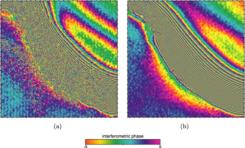
The most direct method to extract the grounding lines is to analyze the double differential interferogram constructed from the two interferograms with the best coherence. Therefore, a coherence map is generated for each interferogram and the corresponding average coherence value is calculated. The results show that the best two interferograms are those from 20200727/20200808 and 20200820/20200901. However, the average coherence is merely an overall evaluation of the quality of interferometric signals. As the input data covers a large area, the interferogram possessing the highest overall coherence may still have some areas with low coherence compared to the other interferograms. This phenomenon is exhibited in Figure 3. Figure 3(a) shows the phase signals extracted from a certain grounding zone area of the double differential interferogram with respect to the two interferograms with the highest average coherence, from which severe interferometric decorrelation is clearly observed. On the other hand, the signal in Figure 3(b) is from another interferogram, and its coherence is well preserved. That is to say, if only the best double differential interferogram is utilized, the grounding line over this area cannot be reliably identified. To overcome this issue, the interferograms with high average coherence values are picked out. Grounding lines are then extracted based on the double differential interferograms constructed from the pairwise combinations of the selected interferograms.

Figure 3. Phase signals in different double differential interferograms: (a) 20200727/20200808–20200820/20200901; (b) 20200504/20200516–20200621/20200703. Although (a) is generated based on the interferograms with the best coherence, the phase signals in localized areas may be poorer than those of (b).

Based on the above discussion, the phase observation of a given pixel in the double differential interferogram with respect to the pth and the qth interferograms can be given as:

(4) ${\varphi }^{pq}(m,n)={\varphi }_{hori}^{pq}(m,n)+{\varphi }_{vert}^{pq}(m,n)+{\varphi }_{atm}^{pq}(m,n)+{\varphi }_{noise}^{pq}(m,n),pq\in \mathrm{\Omega }$(4) where ${\varphi }_{\ast }^{pq}(m,n)={\varphi }_{\ast }^p(m,n)-{\varphi }_{\ast }^q(m,n)$ and Ω is the set of double differential pairs.

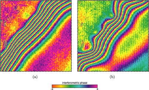
It has been suggested that an ice shelf can be modeled as an elastic beam (Schmeltz, Rignot, and MacAyeal 2002) and the impact of tides can be considered to be the force exerted on the beam (Rack et al. 2017). Tidal motion causes ${\varphi }_{vert}^{pq}$ to vary as an S shaped function along the direction of the beam. In this function, the section with the steepest slope corresponds to the profile of a grounding zone. As a result, high fringe density will be present over grounding zones, as exhibited in Figure 3(b). At present, grounding lines are manually extracted by identifying the location of the first appearance of interferometric fringes in the majority of applications (Rückamp et al. 2019). However, this approach is not suitable for the data in this study due to two reasons: (1) A stack of double differential interferograms is required to be analyzed. It is time-consuming, and the large workload may make it difficult to extract grounding lines correctly; (2) Due to the influence of short term grounding line fluctuations and the presence of ${\varphi }_{hori}^{pq}$ and ${\varphi }_{atm}^{pq}$, the distribution of the fringes on different double differential interferograms may not be consistent (see Figure 4). It is hard to manually identify ground lines with a uniform criterion.

Figure 4. Phase signals in different double differential interferograms: (a) 20200621/20200703-20201019/20201031; (b) 20200621/20200703-20200820/20200901. Tides and local variations in ice thickness can make grounding lines undergo landward/seaward migration during short time periods. Consequently, there should be a position shift between the fringe bands of (a) and (b). Moreover, due to the presence of residual horizontal motions and atmospheric artefacts, (a) and (b) exhibit different fringe shapes.

Note that the density of interferometric fringes is correlated to phase gradients. Therefore, the phase gradients are used for grounding line extraction in this study. In order to suppress the impact of noise on phase gradient estimation, a double differential interferogram is firstly normalized and filtered. Moreover, low quality phase observations are removed, which are identified by using the magnitude of the filtered signal. For a given pixel, its preliminary gradients in azimuth and range directions, $g_{azi}^{pq}(m,n)$ and $g_{ran}^{pq}(m,n)$, are derived by: (5) $g_{azi}^{pq}(m,n)=\frac{\mathrm{\angle }\left(C^{pq}(m+1,n)\times \overline{C^{pq}(m,n)}\right)}{\mathrm{\Delta }{r}_{azi}}$(5)

(6) $g_{ran}^{pq}(m,n)=\frac{\mathrm{\angle }\left(C^{pq}(m,n+1)\times \overline{C^{pq}(m,n)}\right)}{\mathrm{\Delta }{r}_{ran}}$(6) where $C^{pq}(m,n)$ denotes the pixel's complex signal in the differential interferometric pair pq, $\mathrm{\angle }\left(\cdot \right)$ is the angle operator, $\overline{\left(\cdot \right)}$ is the complex conjugate operator, and $\mathrm{\Delta }{r}_{azi}$ and $\mathrm{\Delta }{r}_{ran}$ represent the distances of the neighboring pixels in azimuth and range directions, respectively.

The corresponding gradients in the geographical coordinate system can be calculated using the following equation: (7) $g_x^{pq}(m,n)=g_{azi}^{pq}(m,n)\cos \alpha +g_{ran}^{pq}(m,n)\frac{\sin \alpha }{\sin \theta (m,n)}$(7) (8) $g_y^{pq}(m,n)=g_{azi}^{pq}(m,n)\sin \alpha -g_{ran}^{pq}(m,n)\frac{\cos \alpha }{\sin \theta (m,n)}$(8) Note that $g_x^{pq}(m,n)$ and $g_y^{pq}(m,n)$ can be directly obtained from the geocoded version of the double differential interferogram. However, unnecessary computational costs will be introduced in this case, since the projection of the input data from the radar coordinate to the stereographic coordinate will introduce a large coverage of valueless areas (as shown in Figure 1, the input data only covers the areas indicated by the red dashed rectangle). Moreover, the density of fringes over grounding zone could be high (e.g. larger than 0.5 fringes/pixel). In order to avoid the wrong gradient estimates due to the phase saturation, multilook operations are not recommended to be carried out before the calculation of phase gradients. It should be noted that the preliminary gradients are not reliable due to two reasons: (1) The gradients are actually the wrapped phase differences (i.e. phase modulo 2π) between neighboring pixels. On a small proportion of pixels, inconsistencies may occur between the wrapped gradients and the ‘true’ gradients; (2) The gradients are derived numerically rather than analytically. As mentioned by Schmeltz, Rignot, and MacAyeal (2002), the displacement induced by tides can be depicted as a second-order differentiable function, implying that phase gradients can be considered to be spatially continuous. This feature enables the spatial consistency of the gradients to be enhanced through a spatial filtering. To achieve this goal, a so-called triple differential interferogram is generated. For a given pixel in a triple differential interferogram, its real and imaginary parts are given by $g_x^{pq}(m,n)$ and $g_y^{pq}(m,n)$, respectively. The Goldstein method is applied to filter this complex image Note that, to reduce computational costs, the triple differential interferograms are multilooked with a factor of $5\times 5$ before the filter operations.

The value of a given pixel in a triple differential interferogram can be formulated as: (9) $G^{pq}(m,n)={\mathrm{\Gamma }}^{pq}(m,n)e^{j{\omega }^{pq}(m,n)}$(9) where ${\mathrm{\Gamma }}^{pq}(m,n)$ and ${\omega }^{pq}(m,n)$ denote the magnitude and the phase of the corresponding gradient vector, respectively. As ${\mathrm{\Gamma }}^{pq}(m,n)$ reflects the density of fringes, it will be relatively large over grounding zones. However, classifying grounding zones by simply setting a threshold for the magnitudes of gradient vectors is problematic for two reasons: (1) When the study area is large, it is not reasonable to assume that tides are consistent across all locations; (2) The grounding zone pattern can exhibit rapid variations within localized areas, leading to different fringe densities. The direction of fringe evolution is indicated by ${\omega }^{pq}(m,n)$. Over grounding zones, this direction is generally parallel to the direction of the elastic beam (i.e. perpendicular to the ocean-glacier ice boundary), as the phase contributed by vertical displacements is dominant. With this in mind, a consistency map is calculated based on the following equation: (10) $\xi (m,n)=\frac{\sum _{pq\in \mathrm{\Omega }}\left[e^{j{\omega }^{pq}(m,n)}\times S^{pq}(m,n)\right]}{\sum _{pq\in \mathrm{\Omega }}\left[S^{pq}(m,n)\right]}$(10) where $S^{pq}(m,n)$ is a binary variable. It is equal to 0/1 if $G^{pq}(m,n)$ is an invalid/valid observation.

To assure the basic reliability of $\xi (m,n)$, a pixel is masked out if its corresponding $\sum _{pq\in \mathrm{\Omega }}\left[S^{pq}(m,n)\right]$ is less than a predefined value. To some extent, $\xi (m,n)$ is similar to the ensemble phase coherence (EPC) function (Ferretti, Prati, and Rocca 2000) used in multi-temporal InSAR techniques and can be considered to be an averaging operation along the temporal direction. The negative impacts induced by ${\varphi }_{hori}^{pq}$ and ${\varphi }_{atm}^{pq}$ can be therefore mitigated to some extent. 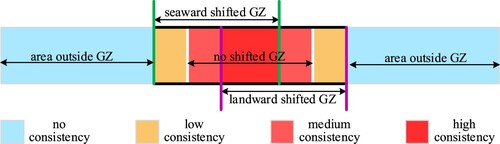The magnitude of $\xi (m,n)$ ranges from 0 to 1. A larger value of this metric represents a better consistency of the direction of fringe evolution. Therefore, the grounding zones can be derived by assigning a threshold of the consistency magnitude. However, this threshold has to be carefully chosen due to short term grounding line fluctuations. Figure 5 is the spatial distribution diagram of the magnitude of $\xi (m,n)$. The white, the purple and the green line pairs indicate the coverages of no shifted, landward shifted and seaward shifted grounding zones, respectively. In the areas colored by light blue, the magnitude of $\xi (m,n)$ tends towards zero as they are located outside the grounding zones. Since the fringe band of every double differential interferogram is present in the deep red area, the highest consistency will be observed over this area. From the deep red area to the yellow areas, the magnitude of $\xi (m,n)$ will drop down due to the decrease in the visit times of fringe bands. Therefore, to take the problem of short term grounding line fluctuations into account, a medium consistency threshold should be utilized.

Figure 5. The spatial distribution diagram of the consistency magnitude over the grounding zone (GZ).

It must be noted that the direction of gradient vectors in a triple differential interferogram might be opposite to that in another one over grounding zones because tides introduce positive/negative ${\varphi }_{vert}^p$. Therefore, the directions of gradient vectors contained in all triple differential interferograms have to be uniformed before the generation of the consistency map. To achieve this goal, the averaged magnitude of the triple differential interferograms is firstly calculated: (11) $\vartheta (m,n)=\frac{\sum _{pq\in \mathrm{\Omega }}\left[{\mathrm{\Gamma }}^{pq}(m,n)\times S^{pq}(m,n)\right]}{\sum _{pq\in \mathrm{\Omega }}\left[S^{pq}(m,n)\right]}$(11) The average magnitude $\vartheta (m,n)$ corresponds to the average fringe density. Therefore, by simply utilizing a threshold of the average magnitude, pixels with a high fringe density are picked out. Next, the double differential interferometric pair with the best coherence is selected as the reference. For each of the other double differential interferometric pairs, a direction consistency angle DCA is calculated by: (12) $DC{A}^{pq}=\mathrm{\angle }\sum _{(m,n)\in \mathrm{\Psi }}{e}^{j\left[{\omega }^{pq}\right(m,n)-{\omega }^{p_r{q}_r}(m,n\left)\right]}$(12) where $p_r{q}_r$ denotes the index of the reference double differential interferometric pair, Ψ is the set of pixels with high fringe density. When $DC{A}^{pq}$ is larger than 90 degrees, the direction of gradient vectors in pq is considered to be opposite to that in the reference pair over grounding zones. In this case, each pixel of the corresponding triple differential interferogram is multiplied by −1.

Due to the removal of low-quality pixels, the consistency map may contain valueless pixels. In this study, the Surfit software is used to interpolate the consistency map. Finally, the consistency map is projected to a polar stereographic coordinate system with a grid size of $25\mathrm{m}\times 25\mathrm{m}$. Note that the proposed method is designed from the perspective of InSAR signal characteristics, and its core idea is to identify the locations and shapes of consistently deforming areas. The above equations do not include any parameters related to glacier physics. Therefore, in theory, the proposed method is independent of regions. If the coherence of the InSAR data can be guaranteed, it is possible to obtain the locations and shapes of the consistently deforming areas with a given consistency threshold.

4. Results and discussion

In this study, the first ten interferograms with the best average coherence values are selected for constructing double differential combinations, which are listed in Table 1. A stack of 45 double differential interferograms is consequently generated. To demonstrate the presence of residual horizontal motion signals, a double differential interferogram generated based on the interferograms (20201218/20201230 and 20201230/20210111) is presented in Figure 6. Interferometric fringes associated with horizontal ice motion can be clearly observed, especially in the floating ice area. Moreover, phase jumps are observed at the demarcation lines between neighboring bursts. They are caused by the non-linear azimuth spectrums of the burst data. Note that Figure 6 is generated based on the interferometric quartet with the shortest temporal baselines.

Figure 6. The double differential interferogram with respect to the pair 20201218/20201230–20201230/20210111. It is in the radar geometry. The interferometric fringes observed over the ice shelf areas, as indicated by the white ellipses, should be mainly attributed to residual horizontal displacements.

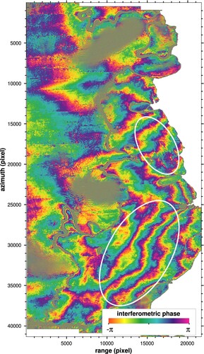
Table 1. The 10 interferometric pairs used for the construction of the double differential interferometric pairs.

interferogram (itf)	SLC1	SLC2	average
ID	acquisition date	acquisition date	coherence
1	20200504	20200516	0.619
2	20200621	20200703	0.624
3	20200727	20200808	0.641
4	20200820	20200901	0.639
5	20201019	20201031	0.598
6	20201218	20201230	0.568
7	20201230	20210111	0.613
8	20210123	20210204	0.592
9	20210815	20210827	0.598
10	20210827	20210908	0.591

The basic idea of the proposed method is to identify grounding zones by taking advantage of the consistency of the direction of the gradient of tide-induced displacements. Therefore, it is crucial that the evolution direction of the fringes over grounding zones is correctly made uniform. In the proposed method, this issue is addressed based on the calculation of DCAs. The resulting DCAs are listed in Table 2. The angle associated with each pair is very close to either 0 or 180 degrees which implies that the evolution direction of the fringes over grounding zones exhibits a fairly consistent pattern along the stack of double differential pairs.

Table 2. The double differential interferometric pairs and their corresponding direction consistency angles (DCAs).

No.	itf1	itf2	DCA	No.	itf1	itf2	DCA	No.	itf1	itf2	DCA
	ID	ID			ID	ID			ID	ID
1	1	2	0.19	16	2	9	181.26	31	5	6	179.76
2	1	3	181.36	17	2	10	181.22	32	5	7	181.44
3	1	4	0.02	18	3	4	0.00	33	5	8	181.10
4	1	5	0.14	19	3	5	0.13	34	5	9	181.27
5	1	6	0.09	20	3	6	0.11	35	5	10	181.30
6	1	7	0.26	21	3	7	0.15	36	6	7	181.11
7	1	8	180.54	22	3	8	0.89	37	6	8	181.19
8	1	9	181.47	23	3	9	0.22	38	6	9	181.33
9	1	10	3.22	24	3	10	0.16	39	6	10	181.34
10	2	3	181.25	25	4	5	181.26	40	7	8	181.11
11	2	4	0.84	26	4	6	181.41	41	7	9	181.18
12	2	5	180.86	27	4	7	181.26	42	7	10	181.19
13	2	6	180.82	28	4	8	181.40	43	8	9	180.96
14	2	7	181.16	29	4	9	181.45	44	8	10	0.56
15	2	8	181.07	30	4	10	181.44	45	9	10	0.08

Notes: In the table header, itf1/itf2 ID is associated with the itf ID in Table 1.

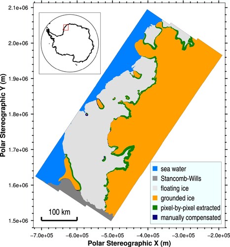
The magnitude of the resulting consistency map in the polar stereographic coordinate system is shown in Figure 7. There is a strong contrast between grounding zones and other areas. By assigning a medium consistency threshold (0.55 is used in this study), the grounding zones are extracted. It can also be observed from the figure that some grounding zone signals are not continuous in space. This is mainly due to two reasons: (1) As the repeat cycle of Sentinel-1B satellite is 12 days, interferometric coherence could not be preserved everywhere; (2) The double differential interferometric signals are saturated over the narrow grounding zones caused by steep topography, which leads to an incorrect estimation of phase gradients. To exhibit the complete distribution of grounding zones, such discontinuities are manually compensated for based on the best double differential interferogram. Fourteen continuous grounding zones with a relatively large coverage are therefore obtained, which are shown in Figure 8. In this figure, the distribution of the grounding zones over the Riiser-Larsen Ice Shelf is clearly presented, and the vast majority of grounding zones are retrieved by the proposed approach.

Figure 7. The magnitude of the consistency map obtained by the proposed method.

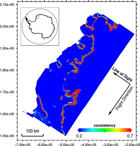
Figure 8. The grounding zones obtained from the consistency map.

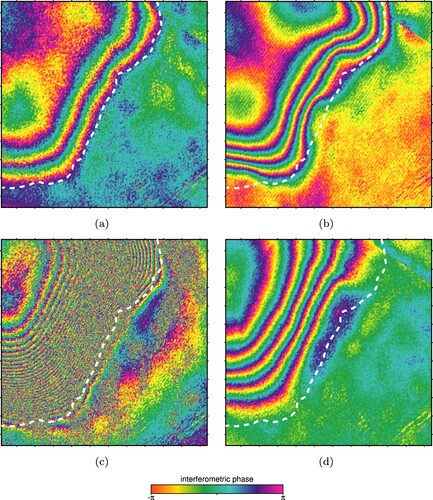
With the use of the resulting grounding zones, vectorized grounding lines are finally obtained based on a simple edge detection between the grounding zones and the grounded ice. The resulting grounding lines are overlaid on a double differential interferogram (20200727/20200808–20210827/20210908), as shown in Figure 9. The figure demonstrates that the resulting grounding lines generally match the boundary of the tide induced interferometric fringes. To further illustrate the performance of the proposed method, other four double differential interferograms are zoomed in over the local region indicated by the white box in Figure 9, as shown in Figure 10. Clearly, due to the tidal differences, the densities of the interferometric fringe bands in the double differential interferograms differ from each other. As can be observed from the Figure 10(a), the resulting grounding line generally matches the interferometric fringe limits. Possibly due to the influences of atmospheric artefacts and residual deformation, the trend of the interferometric fringes in Figure 10(b) differs from that in Figure 10(a,c,d) within local areas. However, the resulting grounding line does not follow this trend. Therefore, the proposed method's ability to deal with the impacts of atmospheric disturbances and residual deformation is demonstrated to some extent. The interferometric coherence of Figure 10(c) is poor. It might be difficult to derive an correct ground line from it via manual delineation operations. However, it can be roughly determined that the fringe limits are located to the landward side of the resulting grounding line. On the contrary, the fringe limits of Figure 10(d) are located to the seaward side of the resulting grounding line. Therefore, it can be concluded that the proposed method, to some extent, is capable of coping with short term grounding line fluctuations.

Figure 9. The resulting grounding lines overlaid on a double differential interferogram.

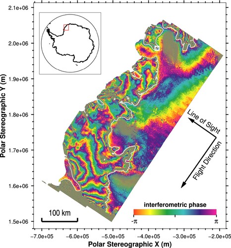
Figure 10. Different zoomed in double differential interferograms over the area indicated by the white box in Figure 9. (a) 20200727/20200808–20210123/20210204; (b) 20200621/20200703–20200820/20200901; (c) 20201218/20201230–20210815/20210827; (d) 20200504/20200516–20200727/20200808.

To further investigate the correctness of the grounding lines extracted by the proposed method, the Antarctic grounding line product from the Making Earth System Data Records for Use in Research Environments (MEaSUREs) (Rignot, Mouginot, and Scheuchl 2016) is imported and shown in Figure 11. In the study area, the MEaSUREs grounding lines were obtained based on ERS-1/2 (acquired between 1992 and 2000) and RadarSAT-1 (acquired in 2000) data. It can be observed that the grounding lines from the proposed method are more complete than those from MEaSUREs. Quantitatively, The total length of the resulting grounding lines with/without manual compensation is approximately 2100 km/1800 km. In contrast, the MEaSUREs product provides grounding lines with a length of approximately 960 km over the study area. In the area indicated by the green cycle, nearly no grounding lines are provided by MEaSUREs. The data loss in this area is believed to be caused by localized interferometric decorrelation of the input SAR data of MEaSUREs. On the other hand, the grounding zone information over this area is preserved by the proposed method. This might be primarily attributed to the use of multiple double differential interferograms, which enables coherent interferometric signals along both spatial and temporal domains to be fully mined. Due to the intersections between the resulting grounding lines and the MEaSUREs product, the minimum deviation is 0. Large deviations are observed in few locations, with a maximum value of approximately 4.6 km. The main reasons for such a deviation could be: (1) The time span between the input data of the two results is approximately 30 years, the grounding line position may have retreated/advanced to a large degree within localized areas; (2) The MEaSUREs product is obtained by using the single double differential interferogram based method, which is susceptible to short term grounding line fluctuations. The average and standard deviations are approximately 0.2 km and 0.14 km, respectively. Therefore, it can be considered that the pattern of the grounding lines obtained by the proposed method almost agrees with that of the MEaSUREs product everywhere. As ERS-1/2 and RadarSAT-1 satellites mainly served between 1990s and 2000s, it can be concluded that the Riiser-Larsen Ice Shelf should have remained relatively structurally static in recent decades.

Figure 11. The comparison between the grounding lines from the proposed method (blue lines) and those from MEaSUREs (red lines). (a) and (b) show examples for good agreements and large deviations between the resulting grounding lines and the MEaSUREs product.

5. Concluding remarks

In this study, Sentinel-1B interferometric SAR images were used to map the grounding lines of the Riiser-Larsen Ice Shelf. Inspired by multi-temporal InSAR techniques, a new method which analyzes a stack of double differential interferograms is proposed for the purpose of the grounding line extraction. The core idea of the proposed method is to estimate the location of grounding zones by making use of the uniformity of the gradient direction of tide-induced vertical deformation. The characteristics of this method can be summarized as follows. First, as grounding lines are the edges of grounding zones in landward direction, the proposed method focuses on the recognition of grounding zones; Second, grounding zones are identified on a pixel-by-pixel basis from a stack of double differential interferograms, effectively bypassing the need for manually delineating operations; Third, the method thoroughly mines coherent signals in spatial and temporal dimensions, which minimizes the loss of grounding zone signals due to interferometric decorrelation; Last, the approach has the potential to minimize the effects of residual horizontal movements and atmospheric artefacts, and is generally capable of addressing short term grounding line fluctuations, since the estimation of direction consistency can be viewed as a temporal averaging process. The grounding lines from the proposed method are much more comprehensive than those from the MEaSUREs. The average and standard deviations between the grounding lines from the proposed method and the MEaSUREs product are approximately 0.2 km and 0.14 km, respectively. Such a good agreement confirms the effectiveness of the proposed method. As the input data of this study and the MEaSUREs were acquired in the 2020s and 1990s–2000s, respectively, it may be concluded that the grounding lines of the Riiser-Larsen Ice Shelf has remained static during 1990–2020.

Disclosure statement

No potential conflict of interest was reported by the author(s).

Data availability statement

The REMA and Sentinel-1B data used in this paper are publicly available and can be accessed https://www.pgc.umn.edu/data/rema and https://search.asf.alaska.edu, respectively.

Additional information

Funding

This research was funded by the National Natural Science Foundation of China (Grant No. 42074034).

References

- Adhikari Surendra, Erik R. Ivins, Eric Larour, Helene Seroussi, Mathieu Morlighem, and Sophie Nowicki. 2014. “Future Antarctic Bed Topography and Its Implications for Ice Sheet Dynamics.” Solid Earth 5 (1): 569–584. https://doi.org/10.5194/se-5-569-2014.
- Berardino Paolo, Gianfranco Fornaro, Riccardo Lanari, and Eugenio Sansosti. 2002. “A New Algorithm for Surface Deformation Monitoring Based on Small Baseline Differential SAR Interferograms.” IEEE Transactions on Geoscience and Remote Sensing 40 (11): 2375–2383. https://doi.org/10.1109/TGRS.2002.803792.
- Bindschadler Robert, Hyeungu Choi, Amy Wichlacz, R. Bingham, Jennifer Bohlander, Kelly Brunt, and Hugh Corr. 2011. “Getting Around Antarctica: New High-resolution Mappings of the Grounded and Freely-floating Boundaries of the Antarctic Ice Sheet Created for the International Polar Year.” The Cryosphere 5 (3): 569–588. https://doi.org/10.5194/tc-5-569-2011.
- Bindschadler Robert, Patricia Vornberger, Andrew Fleming, Adrian Fox, Jerry Mullins, Douglas Binnie, Sara Jean Paulsen, Brian Granneman, and David Gorodetzky. 2008. “The Landsat Image Mosaic of Antarctica.” Remote Sensing of Environment 112 (12): 4214–4226. https://doi.org/10.1016/j.rse.2008.07.006.
- Braun Andreas. 2021. “Retrieval of Digital Elevation Models From Sentinel-1 Radar Data–open Applications, Techniques, and Limitations.” Open Geosciences 13 (1): 532–569. https://doi.org/10.1515/geo-2020-0246.
- Dawson Geoffrey J., and Jonathan L. Bamber. 2020. “Measuring the Location and Width of the Antarctic Grounding Zone Using CryoSat-2.” The Cryosphere 14 (6): 2071–2086. https://doi.org/10.5194/tc-14-2071-2020.
- Dirscherl Mariel C., Andreas J. Dietz, and Claudia Kuenzer. 2021. “Seasonal Evolution of Antarctic Supraglacial Lakes in 2015–2021 and Links to Environmental Controls.” The Cryosphere 15 (11): 5205–5226. https://doi.org/10.5194/tc-15-5205-2021.
- Favier Lionel, Frank Pattyn, Sophie Berger, and Reinhard Drews. 2016. “Dynamic Influence of Pinning Points on Marine Ice-sheet Stability: a Numerical Study in Dronning Maud Land, East Antarctica.” The Cryosphere 10 (6): 2623–2635. https://doi.org/10.5194/tc-10-2623-2016.
- Ferretti Alessandro, Claudio Prati, and Fabio Rocca. 2000. “Nonlinear Subsidence Rate Estimation Using Permanent Scatterers in Differential SAR Interferometry.” IEEE Transactions on Geoscience and Remote Sensing 38 (5): 2202–2212. https://doi.org/10.1109/36.868878.
- Ferretti Alessandro, Claudio Prati, and Fabio Rocca. 2001. “Permanent Scatterers in SAR Interferometry.” IEEE Transactions on Geoscience and Remote Sensing 39 (1): 8–20. https://doi.org/10.1109/36.898661.
- Floricioiu Dana, Kenneth Jezek, Michael Baessler, and Wael Abdel Jaber. 2012. “Geophysical Parameters Estimation With TerraSAR-X of Outlet Glaciers in the Transantarctic Mountains.” In 2012 IEEE International Geoscience and Remote Sensing Symposium, 1565–1568. IEEE.
- Fricker Helen Amanda, Ian Allison, Mike Craven, Glenn Hyland, Andrew Ruddell, Neal Young, Richard Coleman, et al. 2002. “Redefinition of the Amery Ice Shelf, East Antarctica, Grounding Zone.” Journal of Geophysical Research: Solid Earth 107 (B5): ECV1ECV–1. https://doi.org/10.1029/2001JB000383.
- Friedl Peter, Thorsten C. Seehaus, Anja Wendt, Matthias H. Braun, and Kathrin Höppner. 2018. “Recent Dynamic Changes on Fleming Glacier After the Disintegration of Wordie Ice Shelf, Antarctic Peninsula.” The Cryosphere 12 (4): 1347–1365. https://doi.org/10.5194/tc-12-1347-2018.
- Friedl Peter, Frank Weiser, Anke Fluhrer, and Matthias H. Braun. 2020. “Remote Sensing of Glacier and Ice Sheet Grounding Lines: A Review.” Earth-Science Reviews 201:Article ID 102948. https://doi.org/10.1016/j.earscirev.2019.102948.
- Goldstein Richard M., Hermann Engelhardt, Barclay Kamb, and Richard M. Frolich. 1993. “Satellite Radar Interferometry for Monitoring Ice Sheet Motion: Application to An Antarctic Ice Stream.” Science (New York, N.Y.) 262 (5139): 1525–1530. https://doi.org/10.1126/science.262.5139.1525.
- Goldstein Richard M., and Charles L. Werner. 1998. “Radar Interferogram Filtering for Geophysical Applications.” Geophysical Research Letters 25 (21): 4035–4038. https://doi.org/10.1029/1998GL900033.
- Griggs Jennifer A., and J. L. Bamber. 2011. “Antarctic Ice-shelf Thickness From Satellite Radar Altimetry.” Journal of Glaciology 57 (203): 485–498. https://doi.org/10.3189/002214311796905659.
- Han Hyangsun, and Hoonyol Lee. 2014. “Tide Deflection of Campbell Glacier Tongue, Antarctica, Analyzed by Double-differential SAR Interferometry and Finite Element Method.” Remote Sensing of Environment 141:201–213. https://doi.org/10.1016/j.rse.2013.11.002.
- Herzfeld Ute C., Patrick J. McBride, H. Jay Zwally, and John DiMarzio. 2008. “Elevation Changes in Pine Island Glacier, Walgreen Coast, Antarctica, Based on GLAS (2003) and ERS-1 (1995) Altimeter Data Analyses and Glaciological Implications.” International Journal of Remote Sensing 29 (19): 5533–5553. https://doi.org/10.1080/01431160802020510.
- Hillenbrand Claus-Dieter, Michael J. Bentley, Travis D. Stolldorf, Andrew S. Hein, Gerhard Kuhn, Alastair G. C. Graham, and Christopher J. Fogwill. 2014. “Reconstruction of Changes in the Weddell Sea Sector of the Antarctic Ice Sheet Since the Last Glacial Maximum.” Quaternary Science Reviews 100:111–136. https://doi.org/10.1016/j.quascirev.2013.07.020.
- Hogg Anna E., Andrew Shepherd, Noel Gourmelen, and Marcus Engdahl. 2016. “Grounding Line Migration From 1992 to 2011 on Petermann Glacier, North-West Greenland.” Journal of Glaciology 62 (236): 1104–1114. https://doi.org/10.1017/jog.2016.83.
- Howat Ian M., Claire Porter, Benjamin E. Smith, Myoung-Jong Noh, and Paul Morin. 2019. “The Reference Elevation Model of Antarctica.” The Cryosphere 13 (2): 665–674. https://doi.org/10.5194/tc-13-665-2019.
- Joughin Ian, Ben E. Smith, and Waleed Abdalati. 2010. “Glaciological Advances Made with Interferometric Synthetic Aperture Radar.” Journal of Glaciology 56 (200): 1026–1042. https://doi.org/10.3189/002214311796406158.
- Kim Seung Hee, and Duk-jin Kim. 2017. “Combined Usage of Tandem-x and Cryosat-2 for Generating a High Resolution Digital Elevation Model of Fast Moving Ice Stream and Its Application in Grounding Line Estimation.” Remote Sensing 9 (2): 176. https://doi.org/10.3390/rs9020176.
- Le Meur E., M. Sacchettini, S. Garambois, Etienne Berthier, A. S. Drouet, Geoffroy Durand, and D. Young. 2014. “Two Independent Methods for Mapping the Grounding Line of An Outlet Glacier–an Example From the Astrolabe Glacier, Terre Adélie, Antarctica.” The Cryosphere 8 (4): 1331–1346. https://doi.org/10.5194/tc-8-1331-2014.
- Lee Hoonyol, Heejeong Seo, Hyangsun Han, Hyeontae Ju, and Joohan Lee. 2021. “Velocity Anomaly of Campbell Glacier, East Antarctica, Observed by Double-Differential Interferometric SAR and Ice Penetrating Radar.” Remote Sensing 13 (14): 2691. https://doi.org/10.3390/rs13142691.
- Liang Dong, Huadong Guo, Lu Zhang, Haipeng Li, and Xuezhi Wang. 2022. “Sentinel-1 EW Mode Dataset for Antarctica From 2014–2020 Produced by the CASEarth Cloud Service Platform.” Big Earth Data 6 (4): 385–400. https://doi.org/10.1080/20964471.2021.1976706.
- Mikhail Dmitrievskiy, and Kutrunov Vladimir. 2021. “Surfit.” Accessed March 25, 2021. http://surfit.sourceforge.net/surfit/index.html.
- Milillo Pietro, Eric Rignot, Jeremie Mouginot, Bernd Scheuchl, Mathieu Morlighem, Xin Li, and Jacqueline T Salzer. 2017. “On the Short-term Grounding Zone Dynamics of Pine Island Glacier, West Antarctica, Observed with COSMO-SkyMed Interferometric Data.” Geophysical Research Letters 44 (20): 10–436. https://doi.org/10.1002/2017GL074320.
- Moussavi Mahsa, Allen Pope, Anna Ruth W. Halberstadt, Luke D. Trusel, Leanne Cioffi, and Waleed Abdalati. 2020. “Antarctic Supraglacial Lake Detection Using Landsat 8 and Sentinel-2 Imagery: Towards Continental Generation of Lake Volumes.” Remote Sensing 12 (1): 134. https://doi.org/10.3390/rs12010134.
- Rack Wolfgang, Matt A. King, Oliver J. Marsh, Christian T. Wild, and Dana Floricioiu. 2017. “Analysis of Ice Shelf Flexure and Its InSAR Representation in the Grounding Zone of the Southern McMurdo Ice Shelf.” The Cryosphere 11 (6): 2481–2490. https://doi.org/10.5194/tc-11-2481-2017.
- Rebesco Michele, E. Domack, F. Zgur, C. Lavoie, A. Leventer, S. Brachfeld, and V. Willmott. 2014. “Boundary Condition of Grounding Lines Prior to Collapse, Larsen-B Ice Shelf, Antarctica.” Science (New York, N.Y.) 345 (6202): 1354–1358. https://doi.org/10.1126/science.1256697.
- Rignot Eric. 1996. “Tidal Motion, Ice Velocity and Melt Rate of Petermann Gletscher, Greenland, Measured From Radar Interferometry.” Journal of Glaciology 42 (142): 476–485. https://doi.org/10.3189/S0022143000003464.
- Rignot Eric, Jeremie Mouginot, Mathieu Morlighem, Helene Seroussi, and Bernd Scheuchl. 2014. “Widespread, Rapid Grounding Line Retreat of Pine Island, Thwaites, Smith, and Kohler Glaciers, West Antarctica, From 1992 to 2011.” Geophysical Research Letters 41 (10): 3502–3509. https://doi.org/10.1002/2014GL060140.
- Rignot Eric, Jeremie Mouginot, and B Scheuchl. 2011. “Antarctic Grounding Line Mapping From Differential Satellite Radar Interferometry.” Geophysical Research Letters 38 (10). https://doi.org/10.1029/2011GL047109.
- Rignot Eric, Jeremie Mouginot, and Bernd Scheuchl. 2016. “MEaSUREs Antarctic Grounding Line from Differential Satellite Radar Interferometry, Version 2.” Boulder, Colorado USA. NASA National Snow and Ice Data Center Distributed Active Archive Center. https://doi.org/10.5067/IKBWW4RYHF1Q.
- Rignot Eric, Jeremie Mouginot, Bernd Scheuchl, Michiel Van Den Broeke, Melchior J. Van Wessem, and Mathieu Morlighem. 2019. “Four Decades of Antarctic Ice Sheet Mass Balance From 1979–2017.” Proceedings of the National Academy of Sciences 116 (4): 1095–1103. https://doi.org/10.1073/pnas.1812883116.
- Rosenau R., E. Schwalbe, H.-G. Maas, Michael Baessler, and R. Dietrich. 2013. “Grounding Line Migration and High-resolution Calving Dynamics of Jakobshavn Isbræ, West Greenland.” Journal of Geophysical Research: Earth Surface 118 (2): 382–395. https://doi.org/10.1029/2012JF002515.
- Rückamp Martin, Niklas Neckel, Sophie Berger, Angelika Humbert, and Veit Helm. 2019. “Calving Induced Speedup of Petermann Glacier.” Journal of Geophysical Research: Earth Surface 124 (1): 216–228. https://doi.org/10.1029/2018JF004775.
- Sánchez-Gámez Pablo, and Francisco J. Navarro. 2017. “Glacier Surface Velocity Retrieval Using D-InSAR and Offset Tracking Techniques Applied to Ascending and Descending Passes of Sentinel-1 Data for Southern Ellesmere Ice Caps, Canadian Arctic.” Remote Sensing 9 (5): 442. https://doi.org/10.3390/rs9050442.
- Scheuchl B., Jeremie Mouginot, Eric Rignot, M. Morlighem, and Ala Khazendar. 2016. “Grounding Line Retreat of Pope, Smith, and Kohler Glaciers, West Antarctica, Measured with Sentinel-1a Radar Interferometry Data.” Geophysical Research Letters 43 (16): 8572–8579. https://doi.org/10.1002/2016GL069287.
- Schmeltz Marjorie, Eric Rignot, and Douglas MacAyeal. 2002. “Tidal Flexure Along Ice-sheet Margins: Comparison of InSAR with An Elastic-plate Model.” Annals of Glaciology 34:202–208. https://doi.org/10.3189/172756402781818049.
- Schoof Christian. 2007. “Ice Sheet Grounding Line Dynamics: Steady States, Stability, and Hysteresis.” Journal of Geophysical Research: Earth Surface 112 (F3). https://doi.org/10.1029/2006JF000664.
- Thoma Malte, Klaus Grosfeld, and Manfred A. Lange. 2006. “Impact of the Eastern Weddell Ice Shelves on Water Masses in the Eastern Weddell Sea.” Journal of Geophysical Research: Oceans 111 (C12). https://doi.org/10.1029/2005JC003212.
- Yagüe-Martínez Néstor, Pau Prats-Iraola, Fernando Rodriguez Gonzalez, Ramon Brcic, Robert Shau, Dirk Geudtner, Michael Eineder, and Richard Bamler. 2016. “Interferometric Processing of Sentinel-1 TOPS Data.” IEEE Transactions on Geoscience and Remote Sensing 54 (4): 2220–2234. https://doi.org/10.1109/TGRS.2015.2497902.
- Yang Bojin, Shuang Liang, Huabing Huang, and Xinwu Li. 2022. “An Elevation Change Dataset in Greenland Ice Sheet From 2003 to 2020 Using Satellite Altimetry Data.” Big Earth Data1–18. https://doi.org/10.1080/20964471.2022.2116796.
- Zebker Howard A. 2017. “User-Friendly InSAR Data Products: Fast and Simple Timeseries Processing.” IEEE Geoscience and Remote Sensing Letters 14 (11): 2122–2126. https://doi.org/10.1109/LGRS.2017.2753580.
- Zhang Kui, Linlin Ge, Xiaojing Li, and Alex Hay-Man Ng. 2013. “Monitoring Ground Surface Deformation Over the North China Plain Using Coherent ALOS PALSAR Differential Interferograms.” Journal of Geodesy 87 (3): 253–265. https://doi.org/10.1007/s00190-012-0595-y.
- Zhang Kui, Alex Hay-Man Ng, Linlin Ge, Yusen Dong, and Chris Rizos. 2010. “Multi-path PALSAR Interferometric Observations of the 2008 Magnitude 8.0 Wenchuan Earthquake.” International Journal of Remote Sensing 31 (13): 3449–3463. https://doi.org/10.1080/01431161003727804.
- Zhao Jiechen, Jingjing Cheng, Zhongxiang Tian, Xiaopeng Han, Hui Shen, Guanghua Hao, Honglin Guo, and Qi Shu. 2022. “Snow and Ice Thicknesses Derived From Fast Ice Prediction System Version 2.0 (FIPS V2. 0) in Prydz Bay, East Antarctica: Comparison with in-situ Observations.” Big Earth Data 6 (4): 492–503. https://doi.org/10.1080/20964471.2021.1981196.