Classification of hyperspectral images using fusion of CNN and MiniGCN with SVM

ABSTRACT

Convolutional neural networks (CNNs) have gained popularity for categorizing hyperspectral (HS) images due to their ability to capture representations of spatial-spectral features. However, their ability to model relationships between data is limited. Graph convolutional networks (GCNs) have been introduced as an alternative, as they are effective in representing and analyzing irregular data beyond grid sampling constraints. While GCNs have traditionally been computationally intensive, minibatch GCNs (miniGCNs) enable minibatch training of large-scale GCNs. We have improved the classification performance by using miniGCNs to infer out-of-sample data without retraining the network. In addition, fuzing the capabilities of CNNs and GCNs, through concatenative fusion has been shown to improve performance compared to using CNNs or GCNs individually. Finally, support vector machine (SVM) is employed instead of softmax in the classification stage. These techniques were tested on two HS datasets and achieved an average accuracy of 92.80 using Indian Pines dataset, demonstrating the effectiveness of miniGCNs and fusion strategies.

KEYWORDS:

• CNN
• hyperspectral images
• MiniGCN
• SVM

1. Introduction

Geoscience and remote sensing present challenges to land use and land cover classification (Anderson et al. 1976; Zhang et al. 2021), including hyperspectral (HS) data, synthetic aperture radar (SAR) data (Kang et al. 2021), light detection and ranging (LiDAR) data (Huang et al. 2020), and so on. It is easier to distinguish between objects of interest (especially those in spectrally similar classes) when HS images are provided with rich and detailed spectral information (Zhang et al. 2021), as the contiguous shapes of the spectral signatures linked to the pixels can be used to detect more subtle differences. As opposed to RGB/MS imaging, HS imaging allows finer and more accurate identification of materials on the surface of the earth. However, spectrum variability, complicated noise effects, and high spectral mixing amongst materials make it challenging to extract discriminative information from such data (Hong et al. 2019; Bioucas-Dias et al. 2012; Zhang et al. 2023; Zhang et al. 2022).

There have been numerous features extraction (FE) algorithms developed over the years for categorizing HS images (either unsupervised or supervised) (Ghamisi et al. 2017; Hong et al. 2020; Hong et al. 2019; Liu et al. 2019; Liu et al. 2019; Peng and Du 2017; Peng, Sun, and Du 2019; Wang, Peng, and Sun 2019). One of the most useful tools for manually extracting spatial-spectral features from HS photos is the morphological profile (Benediktsson, Aevar Palmason, and Sveinsson 2005).

The support vector machine (SVM) classifier utilized MPs as input vectors, and satisfactory classification results were obtained. The authors developed MPs guided by extremal regions that produce excellent classification results for MS images (Samat et al. 2018). Attribute profiles (APs) and invariant attributes (APs) have been developed as morphological operations-based approaches to improve feature representations (Hong et al. 2020; Wu et al. 2020). There are other methods in FE, such as manifold learning (Hong et al. 2020; Gao et al. 2021) and sparse representation (Chen, Nasrabadi, and Tran 2011), which is based on subspaces. Transform or project the high-dimensional initial space using a low-dimensional representation latent in a subspace. However, the lack of robust data fitting and representation capabilities limits feature discrimination in HS classification tasks. Deep learning (DL) approaches were inspired by deep networks to make significant advances in HS image classification (Li et al. 2019; Chen et al. 2014; Dong et al. 2022) classified dimensionally reduced HS pictures using stacked autoencoder networks derived from principal component analysis (PCA).

In addition, the authors use of convolutional neural networks (CNNs) improved classification results by extracting spatial-spectral information more efficiently from HS images (Chen et al. 2016). With recurrent neural networks (RNNs), spectral signatures can be processed sequentially (Liu et al. 2017; Wu and Prasad 2017). To fully utilize spectral information for high-accuracy HS picture classification, a cascaded RNN was suggested in (Hang et al. 2019). Recent research by Hang et al (Hang et al. 2021)produced state-of-the-art performance by creating multitask generative adversarial networks and offering fresh perspectives on HS picture categorization.

To handle graph structure data (or vertexes), graph convolutional networks (GCNs) (Kipf and Welling 2017) simulate relationships between samples. Thus, GCNs can model long-range spatial relationships in HS images without incorporating the shortcomings of CNNs. HS image categorization currently uses GCNs less than CNNs. The application of GCNs to HSI classification has been discussed in a few papers. A cascading 1-D CNN and GCN model was presented by Shahraki and Prasad (Shahraki and Prasad 2019) for HS image classification. By simultaneously considering spectral and spatial regions, Qin et al. developed a second-order GCN. HS images are segmented using superpixels before being fed into GCN, which reduces computing costs and increases classification accuracy. GCNs may, however, be subject to some limitations due to the following factors.

It is noteworthy that GCNs face a high computational cost when classifying HS images (originating from the adjacency matrix generation), especially when using large-scale HS image sets.

All samples are sent simultaneously to the GCN during full-batch network learning with GCNs. This could negatively affect variable updates, as well as increase memory costs and slow gradient descent.

Furthermore, if a trained GCN-based model is not retrained, it cannot forecast new input samples (out of samples), which significantly impacts GCN applications.

In this study, we offer a straightforward but efficient minibatch GCN to get over these challenges (called miniGCN). It is possible to train miniGCNs based on a downsampled graph (or topological structure), as well as use them directly to predict. In addition to their ability to extract and represent spectrum data from HS images, CNNs and GCNs also possess other capabilities, such as their spatial-spectral characteristics and graph representations (or relations), etc. Our collaborative efforts with the help of SVM will make them even more suitable for HS image categorization by incorporating them. More specifically, this article makes three important contributions.

We conduct a thorough examination of GCNs and CNNs with an emphasis on HS image categorization.

We used miniGCNs, a new supervised variation of GCNs. Moreover, miniGCN training can be done in minibatch form to achieve a more reliable and better local optimum. In contrast to conventional GCNs, miniGCNs are capable of training using training data as well as inferring large-scale data out of sample.

A trainable network comprised of CNNs and miniGCNs uses concatenation fusion techniques to improve HS classification results.

The rest of this article is divided into the following sections. Section 2 goes in-depth literature on knowledge pertaining to GCN and HS image classification. In the framework of a broad end-to-end fusion network, Section III proposes three potential fusion algorithms and expands on the suggested miniGCNs. In Section IV, extensive experiments and analysis are provided. This article’s Section V offers some closing thoughts and suggestions for potential future study projects.

2. Literature review

This section 2.1 discusses the spectral and spatial domains of graph convolutional networks and how they are developed. We evaluate a few sample efforts on the HSI classification task in Section 2.2. In addition, we assess the performance of graph convolutional networks for classification of hyperspectral images.

2.1. Graph convolutional network

Since the theory behind graph convolutional networks has reached its full development, several other fields have made extensive use of this technology. There are a few illustrative works, including natural language processing and recommendation systems (Ying et al. 2018)

Graph neural networks have the advantage of processing graph-structured input directly in non-Euclidean space, as compared to CNN and RNNs. Gori, Monfardini, Scarselli (Gori, Monfardini, and Scarselli 2005) initially put up the idea for it. Convolution on a graph can be split into two classes based on several viewpoints (Zhang, Cui, and Zhu 2022). By first converting the graph signal to the spectral domain, this kind of convolution extracts the convolution from there. From the perspective of the spatial domain, node features are aggregated in spatial graph convolution.

Spectral CNNs (SCNNs) (Bruna et al. 2014) are prominent early works in spectral approaches that convert graph signals into spectral domains via graph Fourier transforms. An enumerated set of learnable parameters that relate to Fourier bases is defined as the convolution kernel in this study. Spectral CNNs, however, have a tight relationship with sample size due to their difficult eigen-decompositions of Laplacian matrices. These models are computationally expensive and prone to overfitting on large graphs. As a result, ChebyNet (Defferrard, Bresson, and Vandergheynst 2016) fitted the frequency response function using Chebyshev polynomials instead of eigen-decomposition steps, resulting in a parameter that is related only to the polynomial order, a parameter much smaller than the sample size, eliminating the need for a complex eigen-decomposition step. The first-order approximation of the polynomial and Kipf and Welling’s (Kipf and Welling 2017) further improvements to ChebyNet led to a more effective graph filtering operation than ChebyNet did.

Convolution on each node in a spatial graph is viewed as linear weighting within neighbors according to the weighting function, which describes how adjacent nodes influence the target node (Xu et al. 2019). As an example, it is used in GraphSAGE (Hamilton, Ying, and Leskovec 2017) to sample neighbor nodes and then aggregate them using aggregation techniques. With self-attention mechanisms, neighbors are grouped in a graph attention network. The authors describe convolution as superimposing many weighting functions on neighbors as an integrated framework of spatial techniques (Monti et al. 2016).

2.2. Hyperspectral image classification

It is crucial to extract features from hyperspectral images before categorizing them. For HSI classification, many feature extraction methods have been effectively applied (Peng and Du 2017). For example, principal component analysis (PCA) can be used for HSI (Licciardi et al. 2012), linear discriminant analysis (LDA) (Izenman 2008) and neighborhood embeddings (NPE) (Xiaofei He, Yan, and Zhang 2005). However, a complex scenario like spectral variability makes it difficult to effectively classify different land-cover groups by relying just on spectral data. As a result, using spatial context information for HSI’s classification task has become a trend that cannot be avoided. Recently, spectral-spatial HSI classification methods have been developed that reveal rich spectral-spatial joint characteristics, including attribute profiles (APs), morphological profiles (MPs), Markov random fields (MRFs), segmentation-based techniques (Zhang et al. 2020), and sparse representation methods (Ding, Pan, and Chong 2020). However, because they use manually created spectral-spatial features, all these approaches perform poorly at identifying small differences between distinct categories or significant variances within the same category.

Deep learning has gained more attention as a cutting-edge solution for a variety of computer vision problems (Zhao et al. 2019) because it can automatically extract useful features, avoiding the laborious hand-crafted feature engineering (Yang et al. 2018). The HSI classification task has recently undergone revolutionary alterations as a result (Audebert, Saux, and Lefevre 2019). Using stacked autoencoders (SAEs), Chen et al. (Chen et al. 2014) learned hierarchical features unsupervised for the first time. Based on these robust features, Chen et al. (Chen, Zhao, and Jia 2015) used the deep belief network to extract robust features, then used logistic regression for classification. Rodriguez, Wiles, and Elman (Rodriguez, Wiles, and Elman 1999) have introduced recurrent neural networks to HSI classification, allowing them to dig for spectral and spatial information on multiple scales and capture spatial dependence between these scales. A generative adversarial network (GAN) was also used for classification of HSI as input by Zhu et al. (Zhu et al. 2018). In recent research, Transformers, which are adept at handling sequence data, have been used to extract spectral information from continuous spectra. As compared to other programs, CNN performed better in the HSI classification job. A CNN-based HSI classification approach can be divided into three categories based on the input data: its spectral version, its spatial version, and its spectral-spatial version.

Each pixel vector serves as the model’s input in the HSI classification technique by using spectral analysis. A five-layer 1-D CNN was suggested by Hu et al. (Hu et al. 2015) to categorize HSI using spectral characteristics. Additionally, Li et al (Li et al. 2017) pixel-pair technique ensures that CNN’s superiority may be effectively utilized by greatly increasing the amount of training samples.

A spatial CNN-based algorithm typically uses 2D CNNs to extract spatial information from HSI. Using PCA to map data into three-dimensional feature space first, Makantasis et al. (Makantasis et al. 2015) extracted spatial features using typical 2D CNN. Additionally, Slavkovikj et al. (Slavkovikj et al. 2015) flattened the original hyperspectral data in accordance with the spatial dimensions. The 2D CNN model used the flattened data as its input. To extract discriminant spatial information. Song et al. 2018 built an extremely deep network using residual modules. Combining multiscale filter banks with multiscale feature extraction frameworks, Gong et al. (Gong et al. 2019) created a unique multiscale feature extraction framework.

CNN-based HSI classification methods can also be classified according to spectral-spatial approach, which uses both spectral and spatial HSI information. One of these techniques that is effective for the HSI classification problem is the 1D + 2D CNN architecture (Mou, Ghamisi, and Zhu 2018; Lee and Kwon 2017). According to Luo et al. (Luo et al. 2018), the first layer in a CNN is convolutional spectral-spatial combined with a 2D CNN to reduce dimensionality. According to their paper Li, Zhang, and Shen (Li, Zhang, and Shen 2017) 3D CNNs can be used directly to process HSI cubes, enabling them to learn more complex 3D patterns with fewer layers and parameters than 1,2,3D CNNs. By combining 3-D CNNs with regularization techniques, Chen et al. (Chen et al. 2016) increased the generalizability of their model.

CNN-based approaches, which are the standard backbone architecture, perform better in HSI classification. Due to the vast parameters, these CNN-based algorithms frequently experience greater computing costs and longer training times. The solution to this problem has been developed in a variety of ways. An example of this is Wang et al. (Wang et al. 2021) who present an HSI classification fusion network based on a lightweight spectral-spatial attention feature that is led by network architecture search (NAS). The ghost-module architecture and a CNN-based HSI classifier are used in Paoletti et al. (Paoletti et al. 2021) technique to provide an effective classification method with good performance while reducing the computing cost. Convolution operations are employed on the regular-grid picture regions using kernels of a predetermined size; therefore, class boundaries will be lost unavoidably.

A recent application of GCN, in which data are represented in a non-Euclidean space and class boundary information can be preserved, is HSI classifying (Ding et al. 2021). An example is Mou et al. (Mou et al. 2020), who extract features from an image by combining convolutional graph layers, which include both labeled and unlabeled pixels as inputs. While Sha et al. (Sha et al. 2021) avoided the fabricated connection weights in the prior GCN, they assigned various weights to various surrounding nodes based on their attention coefficients. However, because of the great spatial resolution in HSI’s many pixels, adjacency matrix calculations are extremely expensive and memory-intensive. To solve this issue, various efforts in the field of remote sensing Saha, Mou, and Zhu (Saha et al. 2021) have been done. However, after super-pixel segmentation, calculating the adjacency matrix among them is the technique that is most frequently used. For instance, Wan et al. (Wan et al. 2021) segmentation of the HSI into a series of homogenous that the SLIC algorithm treats as network nodes. As well as using graph projection and reprojection instead of heuristic superpixel generation techniques to probe long-range context linkages and determine features of regions faithfully. Additionally, Hong et al. (Hong et al. 2021) construction of a subgraph with nodes drawn at random from the HSI reduces the computation of the adjacency matrix. The misclassification brought on by the spectral variation phenomenon can be more effectively reduced by modeling local spatial context relationships in HSI, which was not done in the investigations. We offer an MiniGCN in this paper to address the difficulties mentioned above. As a result, the adjacency matrix’s calculation and memory requirements are drastically lowered, and classification performance is enhanced.

3. Proposed method

3.1. Theory and Basics of CNN and miniGCN

In this section, we thoroughly examine CNNs and GCNs from four distinct viewpoints and enhance an existing GCN technique, referred to as miniGCNs, making them more suitable for HS image classification. Finally, we present fusion method alongwith SVM to form a comprehensive end-to-end fusion network.

3.2. CNNs basics and overview

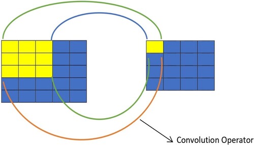
Convolutional Neural Networks (CNNs) are a type of deep learning algorithm primarily used for image classification tasks (Zhang et al. 2023). They consist of several layers, including convolutional layers, activation layers (e.g. ReLU), pooling layers, and fully-connected layers. In a convolutional layer, convolution operator (see in Figure 1) is used to detect patterns in an input image, and a feature map is generated that summarizes the information in a reduced form. Mathematically, the operation of a convolutional layer can be represented as: (1) $F_i=\sigma \left(\sum _{j=1}^n{W}_{i,j}\ast X_j+b_i\right)$(1) Where $F_I$ is the $i^{th}$ feature map, $W_{I,j}$ is the set of weights for the $i^{th}$ filter and $j^{th}$ channel, $X_j$ is the input image or previous layer's output, $\ast$ denotes the convolution operation, $\sigma$ is an activation function (e.g. ReLU), and $b_i$ is a bias term for the $i^{th}$ feature map.

Figure 1. Convolution process (3 × 3 convolutional operator).

Pooling layers reduce the size of the feature map, while activation layers introduce non-linearities into the model. Finally, the fully-connected layer is used to make predictions based on the features extracted by the convolutional and pooling layers. The output of the last pooling layer is typically flattened into a vector and passed through one or more fully-connected layers. Each neuron in a fully-connected layer is connected to all neurons in the previous layer, and its output is computed as. (2) $Y=\sigma (WX+b)$(2) where $Y$ is the output vector, $W$ is the weight matrix, $X$ is the input vector, $\mathit{b}$ is a bias vector, and $\sigma$ is an activation function.

3.3. Graph and miniGCN overview

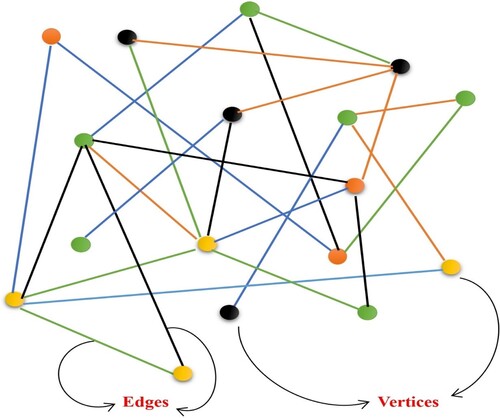
A graph as a data structure that consists of a set of vertices (or nodes) and a set of edges that connect pairs of nodes i.e. $G=(V,E)$. In the context of machine learning, a graph can be used to model relationships between objects (Shahraki and Prasad 2019), such as entities in a social network or regions in an image (see in Figure 2).

Figure 2. Graph structure.

A Graph Convolutional Network (GCN) is a neural network that operates directly on graph data. The GCN is defined as a function that takes a graph $G=(V,E)$ and an input feature matrix $X$ as inputs, and produces an output feature matrix $Z.$ The GCN operates on the graph structure by applying a convolutional operation to the feature matrix, which extracts local features for each node based on its neighboring nodes. This operation can be expressed mathematically as. (3) $Z=f(H,X)$(3) where $H$ is a matrix that represents the graph structure, and $f$ is a non-linear activation function. The matrix $H$ can be constructed using the adjacency matrix $A$ of the graph, which represents the relationships between nodes. The matrix $H$ can be defined as: (4) $H=D^{-{\displaystyle \frac{1}{2}}}\ast A\ast D^{-{\displaystyle \frac{1}{2}}}$(4) Where $D$ is the degree matrix defined as a diagonal matrix with entries.

$D[i,i]=\sum (A[i,j])$ and $\ast$ represents matrix multiplication.

To improve the generalization ability of the graph, the symmetric normalized Laplacian matrix $(L_m)$ can be used instead of $A$. $L_m$ is computed as (5) $L_m=D^{-{\displaystyle \frac{1}{2}}}\ast L\ast D^{-{\displaystyle \frac{1}{2}}}$(5) (6) $L_m=I-D^{-{\displaystyle \frac{1}{2}}}\ast A\ast D^{-{\displaystyle \frac{1}{2}}}$(6) where L is the graph Laplacian matrix, $L=D-A$, and $I$ is the identity matrix

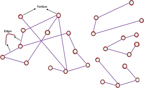
MiniGCN is a simplified version of GCN that reduces the number of layers and parameters, while still retaining some of its capabilities. The approach of batch processing miniGCN (Hong et al. 2021) is employed, whereby batches of pixels are extracted similar to CNNs, and then subgraphs for each batch are created from the adjacency matrix $\mathrm{A}$ (Figure 3).

Figure 3. (a) Full graph (b) MiniGCN.

3.4. Fusionnet architecture

In this research, a hybrid method called FusionNet is employed for the classification of HS images. The FusionNet utilizes a dual-branch architecture that combines the advantages of both miniGCN and CNN networks to extract information from HS images. The framework of FusionNet is illustrated in Figure 4.

Figure 4. Proposed Framework of FusionNet.

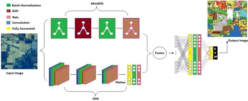
The proposed FusionNet uses HSI images as inputs to two branches: a CNN network that extracts contextual information using convolutional kernels and a miniGCN network that identifies similarities between features using graphs. The miniGCN network includes a batchwise GCN block that receives batchwise pixels and an adjacency matrix representing the nodes and edges of a graph, while the CNN network consists of convolutional layers followed by average pooling of size 2 and an FC layer that reshapes the output of the last convolution to a 1D vector. The reason for using the miniGCN network is that direct fusion with GCN models is not possible due to the pixel-based structure of CNNs. Therefore, a batchwise strategy is employed using miniGCN to achieve GCN capability. The FusionNet method combines the strengths of both CNN and miniGCN networks to extract additional information from the HSI image. The fused output of the two branches is passed through two additional FC layers to further deepen the network, prepare the concatenated features, and ultimately passed through an SVM classifier for classification. This combination of networks, along with the SVM classifier, enables a more comprehensive analysis of the HS image, resulting in improved classification accuracy.

3.5. Dataset

Our proposed algorithms are evaluated using two commonly used HS datasets.

3.5.1. Indian pines dataset

The Indian Pines dataset is a widely used hyperspectral remote sensing image dataset for evaluating and comparing algorithms for hyperspectral image classification (Hanachi et al. 2022). Hyperspectral images provide rich spectral information for each pixel in the image, and the Indian Pines dataset is a high-dimensional dataset, with 224 spectral bands and 145 × 145 pixels. This dataset was collected by the AVIRIS sensor over an agricultural area in Indiana, USA, and contains information about different crops and other land cover types. The Indian Pines dataset is commonly used.

3.5.2. Pavia university dataset

The Pavia University dataset is a hyperspectral remote sensing image dataset that is widely used for evaluating and comparing algorithms for hyperspectral image classification. The Pavia University dataset was collected by the Reflective Optics System Imaging Spectrometer (ROSIS) over an urban area near Pavia, Italy, and contains information about different types of surfaces, including asphalt, meadows, trees, and building materials. The Pavia University dataset is a high-dimensional dataset, with 103 spectral bands and 610 × 340 pixels.

The Pavia University dataset is commonly used in research and development for hyperspectral image processing techniques and is often used as a benchmark for evaluating and comparing algorithms for hyperspectral image classification. The dataset provides a challenging test for algorithms due to its high dimensionality, the variability of the land cover types, and the presence of noise and other artifacts.

4. Experiments

4.1. Implementation detail

The proposed FusionNet model is designed to incorporate diverse information from HS images, utilizing features extracted from both CNNs and GCNs with concatenated fusion strategies through the addition of a fully-connected (FC) fusion layer. In the classification process, SVM is used instead of softmax in the last layer of FusionNet. This decision is motivated by the computational expense of the optimization process of softmax, particularly for large datasets. In contrast, SVM finds the decision boundary that separates classes in a high-dimensional space, resulting in improved classification performance. The configuration of the proposed FusionNet is detailed in Table 1, which outlines the layer-wise network architecture.

Table 1. FusionNet - layer-wise network architecture.

Layer	CNN	MiniGCN
Stage 1	3 × 3 Conv	Batch Normalization
	Batch Normalization	GCN
	2 × 2 AvgPool	Batch Normalization
	ReLU	ReLU
Output size	4 × 4 × 32	128
Stage 2	3 × 3 Conv	-
	Batch Normalization
	2 × 2 AvgPool
	ReLU
Output size	4 × 4 × 64	-
Stage 3	3 × 3 Conv	-
	Batch Normalization
	2 × 2 AvgPool
	ReLU
Output size	1 × 1 × 128	-
Fully connected	Fully Connected	-
	Batch Normalization
	ReLU
Output size	128	-
Fusion	Fully Connected
	Batch Normalization
	ReLU
Output size	256
Output	Fully Connected
	SVM
Output size	Classes

The proposed FusionNet architecture is designed to incorporate diverse information from HSI by combining features extracted from CNN and miniGCN. The network consists of several layers, including three stages of CNN and miniGCN layers, a fully connected layer, a fusion layer, and an output layer. In the first stage, the input HIS is convolved with a 3 × 3 filter, followed by batch normalization, 2 × 2 average pooling, and ReLU activation. This is then fed into a miniGCN layer that applies a graph convolution operation to capture the spatial and spectral relationships between pixels in the HS image. The output of the miniGCN layer is then batch normalized and passed through a ReLU activation function. In the second stage, another CNN layer is applied with the same structure as the first stage, and the output is batch normalized, 2 × 2 average pooled, and passed through a ReLU activation function. In the third stage, another CNN layer is applied with the same structure as the first two stages, and the output is batch normalized, 2 × 2 average pooled, and passed through a ReLU activation function. The output from the third stage is then flattened and passed through a fully connected layer, which is also batch normalized and passed through a ReLU activation function. The output size of this layer is 128. Next, a fusion layer is added, which is another fully connected layer that concatenates the outputs from the CNN and miniGCN layers. This layer is also batch normalized and passed through a ReLU activation function. The output size of this layer is 256. Finally, an output layer is added, which is a fully connected layer with a SVM classifier. The output size of this layer is equal to the number of classes in the classification task.

The following hyperparameters are used in the implementation part as described in the Table 2.

Table 2. Implementation details.

Parameter Name	Description	Parameter Name	Description
Maximum Epochs	200	Learner rate	0.0001
Batch Size	32	Activation Function	ReLU
Optimizer	Adam	L2 regularization	0.001
Momentum	0.9	Shuffle	True
Test size	0.2	K-fold	5

Table 2 provides details about the training parameters for the proposed FusionNet model. The table includes parameters such as Maximum Epochs, Batch Size, Test Size, and Shuffle, which control the network's training process. The optimizer used is Adam with a learning rate of 0.0001 and a momentum of 0.9. K-fold is set to 5 and L2 regularization is 0.001 to prevent overfitting, and the data is shuffled during training to improve performance.

The commonly-used indices i.e. Accuracy and Kappa are used to evaluate the performance of classification. Accuracy measures how well the model is able to classify the data correctly. However, other metrics such as Kappa is also important with accuracy to evaluate the performance of classification models (Sadad et al. 2018). Kappa is a statistical measure that evaluates the agreement between two sets of data. A Kappa value of 1.0 represents perfect agreement between the predicted and actual class labels, while a value of 0 indicates random agreement. A value greater than 0.8 is generally considered to be excellent agreement.

4.2. Performance analysis

The classification scores for each class accuracy and average accuracy generated by the proposed method are presented in Tables 3 and 4, respectively, for the Indian Pines and Pavia University datasets.

Table 3. Results obtained from Indian Pines dataset.

No	Class Name	Accuracy	No	Class Name	Accuracy
1	Corn Notill	79.55	9	Soybean Clean	85.74
2	Corn Mintill	89.59	10	Wheat	97.49
3	Corn	96.47	11	Woods	98.55
4	Grass Pasture	97.66	12	Buildings Grass Trees Drives	92.43
5	Grass Trees	96.69	13	Stone Steel Towers	99.00
6	Hay Windrowed	99.54	14	Alfalfa	96.97
7	Soybean Notill	86.84	15	Grass Pasture Mowed	98.00
8	Soybean Mintill	78.81	16	Oats	91.53
Average Accuracy		92.80
Kappa		92.09

Table 4. Results obtained from Pavia University dataset.

No	Class Name	Accuracy	No	Class Name	Accuracy
1	Asphalt	97.86	6	Bare Soil	73.73
2	Meadows	96.61	7	Bitumen	96.69
3	Gravel	85.59	8	Bricks	99.65
4	Trees	90.00	9	Shadows	93.54
5	Metal Sheets	77.37	-	-	-
Average Accuracy		90.11
Kappa		89.88

In our analysis of Tables 3 and 4, we observed that the accuracy of different classes varied. This variation in classification accuracy among different classes can be attributed to several factors, such as the variability of the training samples for each class and the complexity of the spectral signatures of different land cover classes. Each class has unique spectral characteristics, such as the reflectance values at different wavelengths, that can be challenging to differentiate from other classes. For example, classes in the Table 3 such as Soybean Mintill and Corn Notill may have similar spectral signatures, which can make it difficult to distinguish between them.

In the case of Class No. 8 of Soybean Mintill in the Table 3, which has a lower accuracy of 78.81%, it is composed of pixels belonging to the shadow region. The shadow region can have low reflectance values, making it difficult to distinguish from other classes. This can result in misclassifications and lower accuracy for this class. On the other hand, Class No. 6 of Hay Windrowed has a higher accuracy of 99.54%. This class consists of pixels belonging to the Healthy vegetation class, which has distinct spectral characteristics and is relatively easier to classify. The spectral signature of healthy vegetation is well-defined, with high reflectance values in the visible and near-infrared regions of the electromagnetic spectrum. This makes it easier for the classification algorithm to differentiate between healthy vegetation and other land cover classes. Moreover, we acknowledge that further analysis is required to better understand the factors affecting the classification performance of different classes. However, the proposed FusionNet demonstrated promising results on the Indian Pines dataset, achieving an average accuracy of 92.80 and a Kappa value of 92.89. These results showcase the model's ability to integrate different spectral representations effectively. It is noteworthy that the combined networks, utilizing both CNN and miniGCN features through SVM classification, exhibit an improved ability to identify challenging classes.

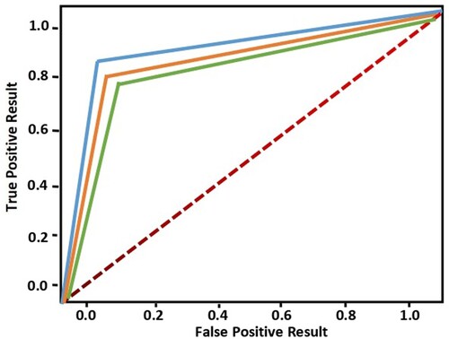
In addition to presenting the classification accuracy results of our proposed method, we have analyzed the performance of our proposed method on the Indian Pines dataset for different ratios of training data, including 80%, 70%, and 60% of the total training samples. The classification accuracy results have been visually depicted using a ROC curve in Figure 5, which clearly illustrates the relationship between the quantity of training data and the performance of our method. Notably, the results consistently demonstrate significant improvement as the amount of training data increases.

Figure 5. Percentage of Training sample (80%, 70%, 60%) using Indian Pines dataset.

4.2.1. Comparison with recent work

Table 5 provides a comprehensive comparison of various classification methods used on the Indian Pines dataset, including the dataset used, methodology, references, and their corresponding average accuracy. The proposed method achieved the highest average accuracy of 92.80%, outperforming all the other methods listed in the table.

Table 5. Results obtained from Pavia University dataset.

Reference	Methodology	Dataset	Average Accuracy
(Sawant and Manoharan 2020)	3D-DCT + SVM	Indian Pines	84.61%
(Zhang et al. 2021)	SSOGCN		92.06%
(Wang, Liu, and Mou 2021)	MSFF + SVM		86.12%
(Anand, Veni, and Aravinth 2021)	3D-DWT + SVM		89.6%
Proposed	FusionNet + SVM		92.80%

Table 6 further illustrates the performance of the different methods on different class labels. The proposed method performed well across most of the class labels, achieving high accuracy scores ranging from 78.81% to 99.54%. Similarly, SSOGCN also demonstrated high accuracy scores for most class labels, with a few exceptions such as Alfalfa where it performed poorly. In contrast, some of the other methods, such as 3D-DCT + SVM and MSFF + SVM, showed lower accuracy scores across most of the class labels.

Table 6. Class Level Comparisons.

Class Labels	Proposed (FusionNet + SVM)	3D-DCT + SVM	SSOGCN	MSFF + SVM	3D-DWT + SVM
Corn Notill	79.55	78.98	87.52	92.64	93.1
Corn Mintill	89.59	75.60	93.46	82.40	94.5
Corn	96.47	66.67	100.0	74.95	96.6
Grass Pasture	97.66	89.64	98.38	96.61	97.3
Grass Trees	96.69	97.09	98.68	98.27	98.6
Hay Windrowed	99.54	98.69	100	99.85	96.9
Soybean Notill	86.84	81.60	92.41	76.58	91.3
Soybean Mintill	78.81	82.29	90.19	94.65	93.0
Soybean Clean	85.74	74.47	95.76	89.37	96.3
Wheat	97.49	92.07	99.35	97.87	96.4
Woods	98.55	96.44	97.12	98.92	92.0
Buildings Grass Trees Drives	92.43	65.58	99.11	79.13	91.2
Stone Steel Towers	99.00	94.59	100.0	88.54	84.6
Alfalfa	96.97	69.44	20.95	96.03	93.3
Grass Pasture Mowed	98.00	81.82	100	68.49	100
Oats	91.53	56.12	100	76.34	100

5. Conclusion

GCN have been shown to effectively capture the structural information of high-dimensional hyperspectral images. However, they come with some limitations, including high storage and computation needs, training issues like exploding gradients, and the need for retraining when new data is added. To address these challenges, this paper proposes a new supervised version of GCN called miniGCN. This approach allows for mini-batch training with SVM, leading to reduced computation and more stable optimization. Moreover, miniGCN enable direct predictions on new input data without the need for retraining. By combining CNN with miniGCN and SVM, the proposed approach achieves improved feature representation for hyperspectral image classification.

Future work will explore integrating miniGCN with other deep networks and implementing advanced fusion techniques to fully exploit the potential of hyperspectral image data.

Disclosure statement

No potential conflict of interest was reported by the author(s).

Data availability statement

We have utilized publicly available datasets: 1. The Indian Pines dataset is accessible at doi:10.4231/R7RX991C. 2. The Pavia University dataset can be found at https://avng.jpl.nasa.gov/pub/ABoselli/f970619t01p02_r02c/.

Additional information

Funding

This paper is supported by Research start up fund for high level talents of FuZhou University of International Studies and Trade [grant no FWKQJ202006], 2022 Guiding Project of Fujian Science and Technology Department [grant no 2022H0026].

References

- Anand, R., S. Veni, and J. Aravinth. 2021. “Robust Classification Technique for Hyperspectral Images Based on 3D-Discrete Wavelet Transform.” Remote Sensing 13 (7), doi:10.3390/rs13071255.
- Anderson, James R., Ernest E. Hardy, John T. Roach, and Richard E. Witmer. 1976. “Land Use and Land Cover Classification System for Use with Remote Sensor Data.” U S Geol Surv, Prof Pap 964. doi:10.3133/PP964.
- Audebert, Nicolas, Bertrand Le Saux, and Sebastien Lefevre. 2019. “Deep Learning for Classification of Hyperspectral Data: A Comparative Review.” IEEE Geoscience and Remote Sensing Magazine 7 (2), doi:10.1109/MGRS.2019.2912563.
- Benediktsson, Jón Atli, Jón Aevar Palmason, and Johannes R. Sveinsson. 2005. “Classification of Hyperspectral Data from Urban Areas Based on Extended Morphological Profiles.” IEEE Transactions on Geoscience and Remote Sensing 43, doi:10.1109/TGRS.2004.842478.
- Bioucas-Dias, José M., Antonio Plaza, Nicolas Dobigeon, Mario Parente, Qian Du, Paul Gader, and Jocelyn Chanussot. 2012. “Hyperspectral Unmixing Overview: Geometrical, Statistical, and Sparse Regression-Based Approaches.” IEEE Journal of Selected Topics in Applied Earth Observations and Remote Sensing, doi:10.1109/JSTARS.2012.2194696.
- Bruna, Joan, Wojciech Zaremba, Arthur Szlam, and Yann LeCun. 2014. “Spectral Networks and Deep Locally Connected Networks on Graphs.” 2nd International Conference on Learning Representations, ICLR 2014 - Conference Track Proceedings.
- Chen, Yushi, Hanlu Jiang, Chunyang Li, Xiuping Jia, and Pedram Ghamisi. 2016. “Deep Feature Extraction and Classification of Hyperspectral Images Based on Convolutional Neural Networks.” IEEE Transactions on Geoscience and Remote Sensing 54 (10), doi:10.1109/TGRS.2016.2584107.
- Chen, Yushi, Zhouhan Lin, Xing Zhao, Gang Wang, and Yanfeng Gu. 2014. “Deep Learning-Based Classification of Hyperspectral Data.” IEEE Journal of Selected Topics in Applied Earth Observations and Remote Sensing 7 (6), doi:10.1109/JSTARS.2014.2329330.
- Chen, Yi, Nasser M. Nasrabadi, and Trac D. Tran. 2011. “Hyperspectral Image Classification Using Dictionary-Based Sparse Representation.” IEEE Transactions on Geoscience and Remote Sensing 49 (10 PART 2), doi:10.1109/TGRS.2011.2129595.
- Chen, Yushi, Xing Zhao, and Xiuping Jia. 2015. “Spectral-Spatial Classification of Hyperspectral Data Based on Deep Belief Network.” IEEE Journal of Selected Topics in Applied Earth Observations and Remote Sensing 8 (6), doi:10.1109/JSTARS.2015.2388577.
- Defferrard, Michaël, Xavier Bresson, and Pierre Vandergheynst. 2016. “Convolutional Neural Networks on Graphs with Fast Localized Spectral Filtering.” In Advances in Neural Information Processing Systems.
- Ding, Yun, Yuanyuan Guo, Yanwen Chong, Shaoming Pan, and Jinpeng Feng. 2021. “Global Consistent Graph Convolutional Network for Hyperspectral Image Classification.” IEEE Transactions on Instrumentation and Measurement 70), doi:10.1109/TIM.2021.3056750.
- Ding, Yun, Shaoming Pan, and Yanwen Chong. 2020. “Robust Spatial-Spectral Block-Diagonal Structure Representation with Fuzzy Class Probability for Hyperspectral Image Classification.” IEEE Transactions on Geoscience and Remote Sensing 58 (3), doi:10.1109/TGRS.2019.2948361.
- Dong, Yanni, Quanwei Liu, Bo Du, and Liangpei Zhang. 2022. “Weighted Feature Fusion of Convolutional Neural Network and Graph Attention Network for Hyperspectral Image Classification.” IEEE Transactions on Image Processing 31: 1559–1572. doi:10.1109/TIP.2022.3144017.
- Gao, Lianru, Danfeng Hong, Jing Yao, Bing Zhang, Paolo Gamba, and Jocelyn Chanussot. 2021. “Spectral Superresolution of Multispectral Imagery with Joint Sparse and Low-Rank Learning.” IEEE Transactions on Geoscience and Remote Sensing 59 (3), doi:10.1109/TGRS.2020.3000684.
- Ghamisi, Pedram, Naoto Yokoya, Jun Li, Wenzhi Liao, Sicong Liu, Javier Plaza, Behnood Rasti, and Antonio Plaza. 2017. “Advances in Hyperspectral Image and Signal Processing: A Comprehensive Overview of the State of the Art.” IEEE Geoscience and Remote Sensing Magazine, doi:10.1109/MGRS.2017.2762087.
- Gong, Zhiqiang, Ping Zhong, Yang Yu, Weidong Hu, and Shutao Li. 2019. “A CNN with Multiscale Convolution and Diversified Metric for Hyperspectral Image Classification.” IEEE Transactions on Geoscience and Remote Sensing 57 (6), doi:10.1109/TGRS.2018.2886022.
- Gori, Marco, Gabriele Monfardini, and Franco Scarselli. 2005. “A new Model for Learning in Graph Domains.” In Proceedings of the International Joint Conference on Neural Networks. Vol. 2, doi:10.1109/IJCNN.2005.1555942.
- Hamilton, William L., Rex Ying, and Jure Leskovec. 2017. “Inductive Representation Learning on Large Graphs.” Advances in Neural Information Processing Systems 2017-December.
- Hanachi, Refka, Akrem Sellami, Imed Riadh Farah, and Mauro Dalla Mura. 2022. “Multi Spectral-Spatial Gabor Feature Fusion Based On End-To-End Deep Learning For Hyperspectral Image Classification.” In 2022 12th Workshop on Hyperspectral Imaging and Signal Processing: Evolution in Remote Sensing (WHISPERS), 1–6. IEEE. doi:10.1109/WHISPERS56178.2022.9955105.
- Hang, Renlong, Qingshan Liu, Danfeng Hong, and Pedram Ghamisi. 2019. “Cascaded Recurrent Neural Networks for Hyperspectral Image Classification.” IEEE Transactions on Geoscience and Remote Sensing 57 (8), doi:10.1109/TGRS.2019.2899129.
- Hang, Renlong, Feng Zhou, Qingshan Liu, and Pedram Ghamisi. 2021. “Classification of Hyperspectral Images via Multitask Generative Adversarial Networks.” IEEE Transactions on Geoscience and Remote Sensing 59 (2): 1424–1436. doi:10.1109/TGRS.2020.3003341.
- Hong, Danfeng, Lianru Gao, Jing Yao, Bing Zhang, Antonio Plaza, and Jocelyn Chanussot. 2021. “Graph Convolutional Networks for Hyperspectral Image Classification.” IEEE Transactions on Geoscience and Remote Sensing 59 (7), doi:10.1109/TGRS.2020.3015157.
- Hong, Danfeng, Xin Wu, Pedram Ghamisi, Jocelyn Chanussot, Naoto Yokoya, and Xiao Xiang Zhu. 2020. “Invariant Attribute Profiles: A Spatial-Frequency Joint Feature Extractor for Hyperspectral Image Classification.” IEEE Transactions on Geoscience and Remote Sensing 58 (6), doi:10.1109/TGRS.2019.2957251.
- Hong, Danfeng, Naoto Yokoya, Jocelyn Chanussot, and Xiao Xiang Zhu. 2019. “An Augmented Linear Mixing Model to Address Spectral Variability for Hyperspectral Unmixing.” IEEE Transactions on Image Processing 28 (4), doi:10.1109/TIP.2018.2878958.
- Hong, Danfeng, Naoto Yokoya, Gui Song Xia, Jocelyn Chanussot, and Xiao Xiang Zhu. 2020. “X-ModalNet: A Semi-Supervised Deep Cross-Modal Network for Classification of Remote Sensing Data.” ISPRS Journal of Photogrammetry and Remote Sensing 167), doi:10.1016/j.isprsjprs.2020.06.014.
- Hu, Wei, Yangyu Huang, Li Wei, Fan Zhang, and Hengchao Li. 2015. “Deep Convolutional Neural Networks for Hyperspectral Image Classification.” Journal of Sensors 2015), doi:10.1155/2015/258619.
- Huang, Rong, Danfeng Hong, Yusheng Xu, Wei Yao, and Uwe Stilla. 2020. “Multi-Scale Local Context Embedding for LiDAR Point Cloud Classification.” IEEE Geoscience and Remote Sensing Letters 17 (4), doi:10.1109/LGRS.2019.2927779.
- Izenman, Alan J. 2008. Modern Multivariate Statistical Techniques. New York, NY: Springer New York. doi:10.1007/978-0-387-78189-1.
- Kang, Jian, Danfeng Hong, Jialin Liu, Gerald Baier, Naoto Yokoya, and Begum Demir. 2021. “Learning Convolutional Sparse Coding on Complex Domain for Interferometric Phase Restoration.” IEEE Transactions on Neural Networks and Learning Systems 32 (2), doi:10.1109/TNNLS.2020.2979546.
- Kipf, Thomas N., and Max Welling. 2017. “Semi-Supervised Classification with Graph Convolutional Networks.” 5th International Conference on Learning Representations, ICLR 2017 - Conference Track Proceedings.
- Lee, Hyungtae, and Heesung Kwon. 2017. “Going Deeper with Contextual CNN for Hyperspectral Image Classification.” IEEE Transactions on Image Processing 26 (10), doi:10.1109/TIP.2017.2725580.
- Li, Shutao, Weiwei Song, Leyuan Fang, Yushi Chen, Pedram Ghamisi, and Jon Atli Benediktsson. 2019. “Deep Learning for Hyperspectral Image Classification: An Overview.” IEEE Transactions on Geoscience and Remote Sensing 57 (9), doi:10.1109/TGRS.2019.2907932.
- Li, Wei, Guodong Wu, Fan Zhang, and Qian Du. 2017. “Hyperspectral Image Classification Using Deep Pixel-Pair Features.” IEEE Transactions on Geoscience and Remote Sensing 55 (2), doi:10.1109/TGRS.2016.2616355.
- Li, Ying, Haokui Zhang, and Qiang Shen. 2017. “Spectral-Spatial Classification of Hyperspectral Imagery with 3D Convolutional Neural Network.” Remote Sensing 9 (1), doi:10.3390/rs9010067.
- Licciardi, Giorgio, Prashanth Reddy Marpu, Jocelyn Chanussot, and Jon Atli Benediktsson. 2012. “Linear Versus Nonlinear PCA for the Classification of Hyperspectral Data Based on the Extended Morphological Profiles.” IEEE Geoscience and Remote Sensing Letters 9 (3), doi:10.1109/LGRS.2011.2172185.
- Liu, Sicong, Qian Du, Xiaohua Tong, Alim Samat, and Lorenzo Bruzzone. 2019. “Unsupervised Change Detection in Multispectral Remote Sensing Images via Spectral-Spatial Band Expansion.” IEEE Journal of Selected Topics in Applied Earth Observations and Remote Sensing 12 (9), doi:10.1109/JSTARS.2019.2929514.
- Liu, Sicong, Daniele Marinelli, Lorenzo Bruzzone, and Francesca Bovolo. 2019. “A Review of Change Detection in Multitemporal Hyperspectral Images: Current Techniques, Applications, and Challenges.” IEEE Geoscience and Remote Sensing Magazine, doi:10.1109/MGRS.2019.2898520.
- Liu, Qingshan, Feng Zhou, Renlong Hang, and Xiaotong Yuan. 2017. “Bidirectional-Convolutional LSTM Based Spectral-Spatial Feature Learning for Hyperspectral Image Classification.” Remote Sensing 9 (12), doi:10.3390/rs9121330.
- Luo, Yanan, Jie Zou, Chengfei Yao, Xiaosong Zhao, Tao Li, and Gang Bai. 2018. “HSI-CNN: A Novel Convolution Neural Network for Hyperspectral Image.” ICALIP 2018 - 6th International Conference on Audio, Language and Image Processing, doi:10.1109/ICALIP.2018.8455251.
- Makantasis, Konstantinos, Konstantinos Karantzalos, Anastasios Doulamis, and Nikolaos Doulamis. 2015. “Deep Supervised Learning for Hyperspectral Data Classification Through Convolutional Neural Networks.” In International Geoscience and Remote Sensing Symposium (IGARSS). Vol. 2015-November, doi:10.1109/IGARSS.2015.7326945.
- Monti, Federico, Davide Boscaini, Jonathan Masci, Emanuele Rodolà, Jan Svoboda, and Michael M. Bronstein. 2016. “Geometric Deep Learning on Graphs and Manifolds Using Mixture Model CNNs.” Proceedings of the IEEE Conference on Computer Vision and Pattern Recognition, November.
- Mou, Lichao, Pedram Ghamisi, and Xiao Xiang Zhu. 2018. “Unsupervised Spectral-Spatial Feature Learning via Deep Residual Conv-Deconv Network for Hyperspectral Image Classification.” IEEE Transactions on Geoscience and Remote Sensing 56 (1), doi:10.1109/TGRS.2017.2748160.
- Mou, Lichao, Xiaoqiang Lu, Xuelong Li, and Xiao Xiang Zhu. 2020. “Nonlocal Graph Convolutional Networks for Hyperspectral Image Classification.” IEEE Transactions on Geoscience and Remote Sensing 58 (12), doi:10.1109/TGRS.2020.2973363.
- Paoletti, Mercedes E., Juan M. Haut, Nuno S. Pereira, Javier Plaza, and Antonio Plaza. 2021. “Ghostnet for Hyperspectral Image Classification.” IEEE Transactions on Geoscience and Remote Sensing 59 (12), doi:10.1109/TGRS.2021.3050257.
- Peng, Jiangtao, and Qian Du. 2017. “Robust Joint Sparse Representation Based on Maximum Correntropy Criterion for Hyperspectral Image Classification.” IEEE Transactions on Geoscience and Remote Sensing 55 (12), doi:10.1109/TGRS.2017.2743110.
- Peng, Jiangtao, Weiwei Sun, and Qian Du. 2019. “Self-Paced Joint Sparse Representation for the Classification of Hyperspectral Images.” IEEE Transactions on Geoscience and Remote Sensing 57 (2), doi:10.1109/TGRS.2018.2865102.
- Rodriguez, Paul, Janet Wiles, and Jeffrey L. Elman. 1999. “A Recurrent Neural Network That Learns to Count.” Connection Science 11 (1), doi:10.1080/095400999116340.
- Sadad, Tariq, Asim Munir, Tanzila Saba, and Ayyaz Hussain. 2018. “Fuzzy C-Means and Region Growing Based Classification of Tumor from Mammograms Using Hybrid Texture Feature.” Journal of Computational Science, doi:10.1016/j.jocs.2018.09.015.
- Saha, Sudipan, Lichao Mou, Xiao Xiang Zhu, Francesca Bovolo, and Lorenzo Bruzzone. 2021. “Semisupervised Change Detection Using Graph Convolutional Network.” IEEE Geoscience and Remote Sensing Letters 18 (4), doi:10.1109/LGRS.2020.2985340.
- Samat, Alim, Claudio Persello, Sicong Liu, Erzhu Li, Zelang Miao, and Jilili Abuduwaili. 2018. “Classification of VHR Multispectral Images Using ExtraTrees and Maximally Stable Extremal Region-Guided Morphological Profile.” IEEE Journal of Selected Topics in Applied Earth Observations and Remote Sensing 11 (9), doi:10.1109/JSTARS.2018.2824354.
- Sawant, Shrutika S., and Prabukumar Manoharan. 2020. “Unsupervised Band Selection Based on Weighted Information Entropy and 3D Discrete Cosine Transform for Hyperspectral Image Classification.” International Journal of Remote Sensing 41 (10), doi:10.1080/01431161.2019.1711242.
- Sha, Anshu, Bin Wang, Xiaofeng Wu, and Liming Zhang. 2021. “Semisupervised Classification for Hyperspectral Images Using Graph Attention Networks.” IEEE Geoscience and Remote Sensing Letters 18 (1): 157–161. doi:10.1109/LGRS.2020.2966239.
- Shahraki, Farideh Foroozandeh, and Saurabh Prasad. 2019. “Graph Convolutional Neural Networks for Hyperspectral Data Classification.” 2018 IEEE Global Conference on Signal and Information Processing, GlobalSIP 2018 - Proceedings. doi:10.1109/GlobalSIP.2018.8645969.
- Slavkovikj, Viktor, Steven Verstockt, Wesley De Neve, Sofie Van Hoecke, and Rik Van de Walle. 2015. “Hyperspectral Image Classification with Convolutional Neural Networks.” In Proceedings of the 23rd ACM International Conference on Multimedia, Vol. 219, 1159–1162. New York, NY, USA: ACM. doi:10.1145/2733373.2806306.
- Wan, Sheng, Chen Gong, Ping Zhong, Shirui Pan, Guangyu Li, and Jian Yang. 2021. “Hyperspectral Image Classification with Context-Aware Dynamic Graph Convolutional Network.” IEEE Transactions on Geoscience and Remote Sensing 59 (1), doi:10.1109/TGRS.2020.2994205.
- Wang, Jianing, Runhu Huang, Siying Guo, Linhao Li, Minghao Zhu, Shuyuan Yang, and Licheng Jiao. 2021. “NAS-Guided Lightweight Multiscale Attention Fusion Network for Hyperspectral Image Classification.” IEEE Transactions on Geoscience and Remote Sensing 59 (10), doi:10.1109/TGRS.2021.3049377.
- Wang, Wenning, Xuebin Liu, and Xuanqin Mou. 2021. “Data Augmentation and Spectral Structure Features for Limited Samples Hyperspectral Classification.” Remote Sensing 13 (4), doi:10.3390/rs13040547.
- Wang, Li, Jiangtao Peng, and Weiwei Sun. 2019. “Spatial-Spectral Squeeze-and-Excitation Residual Network for Hyperspectral Image Classification.” Remote Sensing 11 (7), doi:10.3390/RS11070884.
- Wu, Xin, Danfeng Hong, Jocelyn Chanussot, Yang Xu, Ran Tao, and Yue Wang. 2020. “Fourier-Based Rotation-Invariant Feature Boosting: An Efficient Framework for Geospatial Object Detection.” IEEE Geoscience and Remote Sensing Letters 17 (2), doi:10.1109/LGRS.2019.2919755.
- Wu, Hao, and Saurabh Prasad. 2017. “Convolutional Recurrent Neural Networks ForHyperspectral Data Classification.” Remote Sensing 9 (3), doi:10.3390/rs9030298.
- Xiaofei He, Deng Cai, Shuicheng Yan, and Hong-Jiang Zhang. 2005. “Neighborhood Preserving Embedding.” In Tenth IEEE International Conference on Computer Vision (ICCV’05) Volume 1, 1208-1213 Vol. 2. IEEE. doi:10.1109/ICCV.2005.167.
- Xu, Bingbing, Huawei Shen, Qi Cao, Keting Cen, and Xueqi Cheng. 2019. “Graph Convolutional Networks Using Heat Kernel for Semi-Supervised Learning.” In IJCAI International Joint Conference on Artificial Intelligence Vol. 2019-August, doi:10.24963/ijcai.2019/267.
- Yang, Xiaofei, Yunming Ye, Xutao Li, Raymond Y.K. Lau, Xiaofeng Zhang, and Xiaohui Huang. 2018. “Hyperspectral Image Classification with Deep Learning Models.” IEEE Transactions on Geoscience and Remote Sensing 56 (9), doi:10.1109/TGRS.2018.2815613.
- Ying, Rex, Ruining He, Kaifeng Chen, Pong Eksombatchai, William L. Hamilton, and Jure Leskovec. 2018. “Graph Convolutional Neural Networks for Web-Scale Recommender Systems.” Proceedings of the ACM SIGKDD International Conference on Knowledge Discovery and Data Mining, doi:10.1145/3219819.3219890.
- Zhang, Ziwei, Peng Cui, and Wenwu Zhu. 2022a. “Deep Learning on Graphs: A Survey.” IEEE Transactions on Knowledge and Data Engineering 34 (1), doi:10.1109/TKDE.2020.2981333.
- Zhang, Yuxiang, Wei Li, Weidong Sun, Ran Tao, and Qian Du. 2023a. “Single-Source Domain Expansion Network for Cross-Scene Hyperspectral Image Classification.” IEEE Transactions on Image Processing 32: 1498–1512. doi:10.1109/TIP.2023.3243853.
- Zhang, Yuxiang, Wei Li, Ran Tao, Jiangtao Peng, Qian Du, and Zhaoquan Cai. 2021. “Cross-Scene Hyperspectral Image Classification With Discriminative Cooperative Alignment.” IEEE Transactions on Geoscience and Remote Sensing 59 (11): 9646–9660. doi:10.1109/TGRS.2020.3046756.
- Zhang, Yuxiang, Wei Li, Mengmeng Zhang, Ying Qu, Ran Tao, and Hairong Qi. 2021. “Topological Structure and Semantic Information Transfer Network for Cross-Scene Hyperspectral Image Classification.” IEEE Transactions on Neural Networks and Learning Systems, 2817–2830. doi:10.1109/TNNLS.2021.3109872.
- Zhang, Yuxiang, Wei Li, Mengmeng Zhang, Shuai Wang, Ran Tao, and Qian Du. 2022. “Graph Information Aggregation Cross-Domain Few-Shot Learning for Hyperspectral Image Classification.” IEEE Transactions on Neural Networks and Learning Systems, 1–14. doi:10.1109/TNNLS.2022.3185795.
- Zhang, Yuxiang, Kang Liu, Yanni Dong, Ke Wu, and Xiangyun Hu. 2020. “Semisupervised Classification Based on SLIC Segmentation for Hyperspectral Image.” IEEE Geoscience and Remote Sensing Letters 17 (8), doi:10.1109/LGRS.2019.2945546.
- Zhang, Minghua, Hongling Luo, Wei Song, Haibin Mei, and Cheng Su. 2021. “Spectral-Spatial Offset Graph Convolutional Networks for Hyperspectral Image Classification.” Remote Sensing 13 (21): 4342. doi:10.3390/rs13214342.
- Zhang, Yuxiang, Mengmeng Zhang, Wei Li, Shuai Wang, and Ran Tao. 2023. “Language-Aware Domain Generalization Network for Cross-Scene Hyperspectral Image Classification.” IEEE Transactions on Geoscience and Remote Sensing 61: 1–12. doi:10.1109/TGRS.2022.3233885.
- Zhao, Zhong Qiu, Peng Zheng, Shou Tao Xu, and Xindong Wu. 2019. “Object Detection with Deep Learning: A Review.” IEEE Transactions on Neural Networks and Learning Systems, doi:10.1109/TNNLS.2018.2876865.
- Zhu, Lin, Yushi Chen, Pedram Ghamisi, and Jón Atli Benediktsson. 2018. “Generative Adversarial Networks for Hyperspectral Image Classification.” IEEE Transactions on Geoscience and Remote Sensing 56 (9).