Spatiotemporal dynamics of population density in China using nighttime light and geographic weighted regression method*

ABSTRACT

The distribution and dynamic changes of regional or national population data with long time series are very important for regional planning, resource allocation, government decision-making, disaster assessment, ecological protection, and other sustainability research. However, the existing population datasets such as LandScan and WorldPop all provide data from 2000 with limited time series, while GHS-POP only utilizes land use data with limited accuracy. In view of the limited remote sensing images of long time series, it is necessary to combine existing multi-source remote sensing data for population spatialization research. In this research, we developed a nighttime light desaturation index (NTLDI). Through the cross-sensor calibration model based on an autoencoder convolutional neural network, the NTLDI was calibrated with the same period Visible Infrared Imaging Radiometer Suite Day/Night Band (VIIRS-DNB) data. Then, the geographically weighted regression method is used to determine the population density of China from 1990 to 2020 based on the long time series NTL. Furthermore, the change characteristics and the driving factors of China’s population spatial distribution are analyzed. The large-scale, long-term population spatialization results obtained in this study are of great significance in government planning and decision-making, disaster assessment, resource allocation, and other aspects.

KEYWORDS:

• Nighttime light
• Population density
• Geographically weighted regression
• Population spatialization
• Driving force analysis

1. Introduction

Grid population data can indicate the intensity and scope of human activities, thus accurate description of population distribution information is of great importance to the development of human society sustainable development such as urban planning, resource allocation, government decision-making, disaster assessment, emergency evacuation management, and ecological protection (Cheng, Wang, and Ge 2022; Gaughan et al. 2016; Guo et al. 2023; Huang et al. 2021; Linard et al. 2010; Linard and Tatem 2012; Shang et al. 2021; Ye et al. 2019). At present, most countries and regions in the world obtain population data mainly through sampling surveys and general censuses (Azar et al. 2013; Daniele, Deborah, and Sliuzas 2020; Qiu et al. 2022). Although census data have the advantages of authority, standardization, and system, they are usually summarized by administrative agencies level by level, which has the problems of low temporal resolution, long update cycle, and coarse spatial resolution (Harvey 2002; Wardrop et al. 2018). Population spatialization involves allocating administrative division data to a grid of a certain size according to the model, which makes up for the defects and deficiencies of demographic data and can be combined with other spatial datasets for analysis. It is also crucial for promoting the development of population-related fields (Leyk et al. 2019; Li and Zhou 2018; Stevens et al. 2020).

Remotely sensed data, especially nighttime light (NTL) data, have been widely used in the research of large-scale and long-time population spatialization (Levin et al. 2020; Levin and Zhang 2017; Li and Zhou 2018; Sutton et al., 2001; Sutton et al. 1997). As one kind of satellite NTL data, the Defense Meteorological Satellite Program Operational Linescan System (DMSP-OLS) has long time series data, which has been used in many population spatialization research (Alahmadi et al., 2021b; Amaral et al. 2006; Huang et al. 2016; Li and Zhou 2018; Wang et al. 2018; Ye et al. 2019). There are also many research that combine this data with other remote sensing data and socio-economic data to improve the accuracy of population spatialization, such as land use data, geospatial big data etc. (Huang et al. 2014; Sun et al. 2017; Wang et al. 2018; Ye et al. 2019). However, DMSP-OLS data itself also has many problems. For example, there are inconsistencies in the DMSP-OLS digital number (DN) products obtained by the same sensor at different times and different sensors at the same time (Elvidge et al. 1999; Elvidge et al. 2013a). Moreover, due to the low quantization level of the data, the data has serious overflow and saturation phenomenon (Jing et al. 2015; Letu et al. 2012; Sun et al. 2017). At present, many calibration methods have been proposed to solve the above problems (Zhou et al. 2014; Zhuo et al. 2009; Zhuo et al. 2015). However, this data has stopped updating in 2013, which prevented the application of longer time series research (Elvidge et al. 2013a). The Suomi National Polar-orbiting Partnership (NPP) Visible Infrared Imaging Radiometer Suite Day/Night Band (VIIRS-DNB) has high spatial resolution, and there is no problem of saturation (Elvidge et al. 2013a; Elvidge et al. 2013b; Elvidge et al. 2022; Miller et al. 2012). Since the availability of data in 2012, it has also been widely used in social and economic fields (Guo et al. 2015; Guo, Zhang, and Gao 2018; Ma et al. 2014; Shi et al. 2014; Zhao et al. 2020b). But its time span is still relatively limited, and it is only suitable for population and socio-economic research in recent years (Alahmadi et al. 2021a; Alahmadi et al. 2023; Guo et al. 2022).

In view of the above problems, it is necessary to combine DMSP-OLS and VIIRS-DNB to establish a longer time series of NTL data for socio-economic research (Yuan et al. 2022). The short overlap of the two types of NTL data from 2012 to 2013 provides the basis for generating new NTL data, which is an important prerequisite for mapping the population distribution in a long time series (Lu et al. 2021; Lv et al. 2020; Yong et al. 2022; Zhao et al. 2019; Zhao et al. 2020a; Zheng, Weng, and Wang 2019). Wu et al. (2021) tried to combine the two kinds of NTL data, and used the quadratic model based on the ‘pseudo-invariant pixel’ method to build a new NTL data with a resolution of 1000 m in China from 1992 to 2019. However, this research does not solve the problem of data saturation, and the resolution is still low (1000 m). Low-resolution data is usually more suitable for large-scale and long-term series research to reduce cloud interference, while high-resolution data can provide richer and more detailed image information. Therefore, large-scale research should strive to improve image resolution while also considering long-term sequences to minimize the impact of external environment on images. Using auxiliary data such as vegetation index can reduce the saturation of NTL and improve the spatial resolution, which has been proved by many studies (Guo et al. 2018a; Guo et al. 2022; Guo, Lu, and Kuang 2017; Guo et al. 2015; Lu et al. 2008). Chen et al. (2021) used MODIS normalized difference vegetation index (NDVI) as auxiliary data and combined with DMSP-OLS to obtain the initial non-saturated NTL, and then the autoencoder (AE) method was used to calibrate the above combined variable to obtain the global 500 m NTL data from 2000 to 2018. However, due to the availability of MODIS data (released in 2000), the above 500 m NTL data between 1992 and 2000 is still unavailable, which limits the application of this method in longer time and higher spatial resolution studies. Therefore, it is very urgent to use other auxiliary data to establish a long-time and non-saturated NTL data, especially for the population spatialization research that relies heavily on remote sensing data.

Population spatial models have gone through a long process of development. From the traditional population density model, spatial interpolation has been gradually developed in the regression model. The geographically weighted regression model (GWR) is a local linear regression method derived from spatial transformation relationship. Each part of its research area produces a regression model describing local relationships, which can better explain the local spatial relationship and spatial heterogeneity of variables (Chu et al. 2019; Huang et al. 2018; Xiong et al. 2019). Therefore, it is suitable for the spatialization research of population distribution in long time series.

In our study, we aim to explore a combination index which combine DMSP-OLS data with MODIS NDVI data and Landsat NDVI data respectively to eliminate the saturation and improve the spatial resolution. In addition, the relationship between the combination index based on DMSP-OLS and the VIIRS-DNB data is established based on time overlap of 2012 and 2013. These two types of datasets are cross-corrected to obtain temporally extended NTL at 500 m spatial resolution (1992-2020). Then, the land use/cover data which has been proved very useful in population spatialization research is selected, the NTL data products and corresponding demographic data in 1990, 2000, 2010, and 2020 are also selected and incorporated into the GWR model to spatially transform the county-level administrative census data into a grid level of 500 m resolution. Finally, we explore the change characteristics of China's population density in a long time series and the driving factors leading to population change.

2. Study area and datasets

2.1 Study area

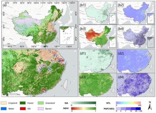
China is in the East Asia and is the third largest country in the world by area (Figure 1). It is also the most populous country in the world with a total population of over 1.4 billion, accounting for nearly 20% of the world's total population. The distribution of China's population presents obvious regional and urban-rural differences. Therefore, accurate long-term mapping studies of China's population can not only help to better understand the distribution of the population and grasp the population change trends in various regions, but also evaluate the economic needs and development potential of different regions.

Figure 1. Study area and datasets (a) the spatial distribution of land use/cover in China, (b1) the spatial distribution of impervious surfaces area, (b2) the spatial distribution of the nighttime light data, (b3) the spatial distribution of NDVI, and (b4) the county-level population statistics in China. (c) a zoomed-in map of the southeast region for (a), and (d1–d4) zoomed-in maps of the southeast region for (b1–b4).

2.2 Datasets and preprocessing

Four types of datasets were selected for this research, including demographic data, NTL (DMSP-OLS, VIIRS-DNB), NDVI (MODIS NDVI, Landsat NDVI), and land use/cover data (Table 1).

Table 1. Description of the datasets for population spatialization.

Datasets	Time	Sources
Population	1990, 2000, 2010, 2020	National Bureau of Statistics of China (http://www.stats.gov.cn/tjsj/)
Administrative Boundary	2020	National Fundamental Geography Information System (http://nfgis.nsdi.gov.cn/)
DMSP-OLS	1992–2013	The National Geographic Data Center, USA (https://ngdc.noaa.gov/eog/dmsp/download_radcal.html/)
VIIRS-DNB	2012–2013, 2020	Payne Institute for Public Policy (https://eogdata.mines.edu/products/vnl/)
MODIS NDVI	2000–2013	Google Earth Engine Platform (https://code.earthengine.google.com/)
Landsat NDVI	1989–2000	Google Earth Engine Platform (https://code.earthengine.google.com/)
Land use/cover	1990, 2000, 2010, 2020	National Land Use/cover Database, China (https://www.resdc.cn/)

The earliest digital version of DMSP-OLS was released in 1992, and we use the 1992 NTL data here to map the population density in 1990 due to the close proximity of the time. Because different source data are used, it is critical to reproject all data to the same Albers coordinate system.

China conducted seven national censuses in 1953, 1964, 1982, 1990, 2000, 2010 and 2020. The demographic data of four periods from the National Bureau of Statistics of China from 1990 to 2020 are used in this study, Hong Kong, Macao, and Taiwan are not included. The administrative boundary vector data (1:4,000,000) used was obtained from the National Fundamental Geography Information System.

The DMSP-OLS data used (1992–2013) are from the National Geophysical Data Center. The pixel value range is from 0 to 63 with 30arc second resolution, and we resampled the data to a 1000 m spatial resolution.

The annual VIIRS-DNB data from 2012 to 2020 are from Colorado University of Mining and Technology. Their spatial resolution is 15 arc-second, which is close to a spatial resolution of 500 m. We removed extremely low background noise in the VIIRS-DNB data using the threshold method (Shi et al. 2014). Pixels with DN values less than 0.3 nanoWatts/(cm2.sr) in the image are assigned a value of 0. The maximum value was set to 100 nanoWatts/(cm2.sr). Here the numbers represent original VIIRS-DNB radiation values which have been multiplied by 1E9.

The land use/cover data used in this research were obtained from the Resource and Environmental Science Data Center. According to the classification system, the datasets were divided into six categories and 25 subcategories. The accuracy of these datasets exceeds 95%, and the spatial resolution is 30 m (Liu et al. 2014; Zhang et al. 2014). We extracted the raster layer of urban, rural, industrial, and traffic construction land as the impervious surface areas (ISAs). Then, we resampled the ISAs to 25 m spatial resolution and aggregated to 500 m spatial resolution to maintain consistency with the long time series NTL data.

The MODIS NDVI data between 2000 and 2013 were obtained from MODIS MOD13A1 products, for which the spatial resolution is 500 m. We used the Google Earth Engine (GEE) platform to calculate the annual mean value according to the monthly NDVI product. The Landsat NDVI data between 1989 and 2000 were from Landsat LT05 products, for which the spatial resolution is 30 m. We first calculated the NDVI of each image. In order to eliminate the influence of data edge unsmooth, we used the three-year average method to compensate. For example, in order to obtain the Landsat NDVI data in 1990, we can select the data from 1989 to 1991, and then take the average value as the NDVI value in 1990. The annual mean value through the GEE platform using the mean algorithm shown in Equation (1). To match the NTL data, the Landsat NDVI data were degraded to 500 m spatial resolution. (1) $NDVI=\mathrm{mean}[NDV{I}_1,NDV{I}_2,\dots ,NDV{I}_n].$(1)

3. Methods

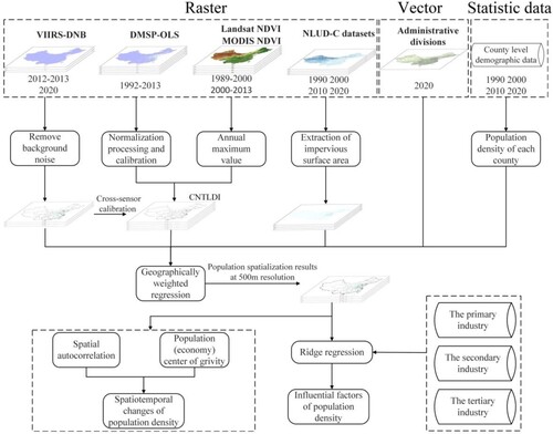
This study can be divided into four main parts: (1) Improvement of DMSP-OLS time series data and connection with VIIRS-DNB data in time series, and establishment of long time series and non-saturated NTL dataset; (2) Determination of grid population distribution; (3) Analysis of the change characteristics of population distribution; (4) Analysis of the driving factors of population distribution change. The calibration of NTL data includes self-calibration of DMSP-OLS, solving saturation and overflow problems and improve the spatial resolution, and cross-sensor calibration of NTLDI and VIIRS-DNB data. Then, the population distribution was obtained using the GWR model, with the demographic data as the dependent variable and the VIIRS-DNB, ISAs, and calibrated NTLDI (CNTLDI) as independent variables. Furthermore, the change characteristics of long-time series population distribution were analyzed through spatial autocorrelation and population center of gravity (PCG). Finally, the ridge regression model was selected to analyze the driving factors of population distribution. The flowchart is shown in Figure 2.

Figure 2. Population spatialization and spatiotemporal changes in population density.

3.1 Improvement of DMSP-OLS time series data

The NTL data are a reflection of human activities in geographical space and can be used for population spatialization analysis. DMSP-OLS (1992–2013) and VIIRS-DNB (2012-present) can provide long-time and global-scale NTL data, but there are large differences between them because they are associated with different sensors, the specific differences are as follows: (1) The quantification level of DMSP-OLS data is low, and there are serious saturation and overflow problems. (2) The NTL intensity detected by DMSP-OLS and VIIRS-DNB differ for the same pixel at the same time. (3) They have different spatial resolutions. Therefore, it is difficult to directly use these two sets of data in long-time study. The saturation problem of DMSP-OLS data must be solved, and the resolution and change information in the two sources of data need to be unified.

3.1.1 Self-calibration of DMSP-OLS datasets

Due to the different atmospheric conditions, lack of onboard calibration, satellite displacement, and sensor degradation, there are inconsistencies in DN values for the same sensor at different times and different sensors at the same time, resulting in the incompatibility of DMSP-OLS time series. To solve this problem in this study, a stepwise calibration scheme is adopted (Liu et al. 2012; Zhang, Pandey, and Seto 2016). A binomial regression model (Equation (2)) was used to establish the relationship between two satellites launched successively in each pair, and the problem of time inconsistency can be improved through sequential calibration (Li and Zhou 2017). Here, the calibrated DMSP data are recorded as CDMSP, and the specific correction coefficient is shown in Table 2. The calibrated NTL time series has the advantage of higher consistency and fewer DN values modified, which is crucial for dynamic research: (2) $D{N}_{ref}=a_0+a_{1}DN+a_{2}D{N}^2,$(2) where $D{N}_{ref}$ is the DN value after calibration, DN is the digital number value of the original image, and $a_0,a_1,a_2$ are calibration coefficients.

Table 2. Coefficients adopted for calibration of DMSP-OLS data.

Year	Satellite	The first step			The second step
		$a_0$	$a_1$	$a_2$	$a_0$	$a_1$	$a_2$
1992–1994	F10	0	1	0	0	1	0
1994–1999	F12	0	1	0	0	1	0
1997–2003	F14	−0.0781	1.4588	−0.0073	0	1	0
2000–2003	F15	0	1	0	0	1	0
2003–2007	F15	−0.4597	1.714	−0.0114	0	1	0
2004	F16	0.1194	1.2265	−0.0041	−1.2802	1.3313	−0.0055
2005	F16	−0.3209	1.4619	−0.0072	−1.2802	1.3313	−0.0055
2006	F16	0.0877	1.1616	−0.0021	−1.2802	1.3313	−0.0055
2007	F16	0	1	0	−1.2802	1.3313	−0.0055
2008	F16	0.1100	1.0513	−0.001	−1.2802	1.3313	−0.0055
2009	F16	0.6294	1.1188	−0.0024	−1.2802	1.3313	−0.0055
2010	F18	−0.0861	0.821	0.002	0	1	0
2011–2013	F18	0	1	0	0	1	0

In addition, the DMSP-OLS data also have the problem of saturation, and the spatial heterogeneity of population distribution cannot be reflected in these saturated areas. Therefore, this paper proposes a nighttime light desaturation index (NTLDI), in which calibrated DMSP-OLS and NDVI data are combined. This index is used to modify DMSP-OLS data to improve the spatial heterogeneity and resolution of population distribution. The NTLDI is proposed based on the negative correlation relationship between urban characteristics and vegetation, and the formula is as follows: (3) $CDMS{P}_{nor}=CDMSP/63.0,$(3) (4) $NTLDI=(1-NDV{I}_{max})\ast EXP(1+CDMS{P}_{nor})),$(4)

where $CDMSP$ refers to the DMSP-OLS data after annual calibration, $CDMS{P}_{nor}$ refers the normalized $CDMSP$, and $NDV{I}_{mean}$ refers to the annual mean of NDVI (including MODIS NDVI and Landsat NDVI). Research shows that NTL and vegetation have an opposite relationship in the representation of urban areas (Guo, Zhang, and Gao 2018; Guo et al. 2022; Lu et al. 2008), thus, $(1-NDV{I}_{mean})$ can be used as an adjustment factor for DMSP-OLS data. NTLDI can effectively eliminate the saturation of DMSP-OLS and increase the heterogeneity of urban central areas.

3.1.2 Cross-calibration of DMSP-OLS with VIIRS-DNB

The inconsistency between DMSP-OLS and VIRS-DNB data is more serious than that within the DMSP-OLS data. The DMSP-OLS data are recorded as DN values, while the VIIRS-DNB data are the radiation intensity after on-orbit radiation correction. Therefore, it is necessary to calibrate these two types of datasets and generate consistent and temporally extended NTL remotely sensed images (1992-present). To solve this problem, we first combined the DMSP-OLS with NDVI, and produced the non-saturated NTLDI data with 500 m spatial resolution, we then used a cross-sensor calibration model based on the AE model to generate calibrated NTLDI product according to the corresponding VIIRS-DNB data of the calendar year 2013 (Chen et al. 2021). The steps for corrected are as follows: (1) The NTLDI data of 2013 were taken as input training data in the network, and the annual composited VIIRS-DNB data were taken as the training goal in the AE model. (2) The model was used to simulate the NTLDI data of 2012 and precision verification was conducted with the annual composited VIIRS-DNB of 2012. (3) Since there was no DMSP-OLS data in 1990, the three-year average Landsat NDVI from 1989 to 1991 was selected as the auxiliary data for the desaturation of DMSP-OLS data in 1992, so the generated NTLDI was closer to the real data in 1990. The NTLDI data from 1992 to 2013 were input into the AE model, and the time series CNTLDI data eventually produced.

3.2 Population spatialization

Geographically weighted regression (GWR) is a spatial analysis technology commonly used in geography and spatial pattern analysis (Wang et al. 2014). The spatial and geographical location of variables are added to the GWR model when calculating the regression parameters (Hu et al. 2012). At present, this model has become one of the main methods to explore the nonstationarity of spatial relations and is widely used in urban research, social economics, and population spatialization (Guo et al. 2023; Zhang, Shen, and Sun 2021; Zhou, Wang, and Fang 2019). It can be expressed as follows: (5) $P_i=a_0(u_i,v_i)+\sum _{k=1}^n{a}_k(u_i,v_i)x_{ik}+{\epsilon }_i,$(5) where $(u_i,v_i)$ represents the geographical coordinate of the ith sample point, $P_i$ is the estimated value, and ${\beta }_k(u_i,v_i)$ represents the kth estimated parameter. $x_{ik}$denotes the value of kth independent variable, $n$ is the number of independent variables, and ${\epsilon }_i$ is the random error.

Before conducting linear regression model, it is crucial to perform multicollinearity analysis on the characteristic variable. When severe multicollinearity exists, the independent variables are interdependent and vary with each other, which leads to the inability to obtain the true relationship between the independent and dependent variables. Therefore, before conducting geographically weighted regression model, we use the variance inflation factor (VIF) to test multicollinearity issues of the characteristic variables (O’brien 2007). The VIF depicts the degree of linear correlation between each variable. It is generally believed that when the VIF is greater than 10, there is a multicollinearity problem. $VI{F}_i={\displaystyle \frac{1}{1-R_i^2},}$where, $R_i^2$.represents the coefficient of multiple correlation when one independent variable is regressed against the other independent variables. The tolerance is calculated as $1-R_i^2$, which is inversely proportional to VIF.

In this study, the optimal bandwidth is obtained by the corrected Akaike information criterion (AICc). The population spatialization model is set as follows: The mean value of administrative district population is taken as the dependent variable, and the mean values of CNTLDI and ISAs are the independent variables. The NTL can effectively distinguish between urban and rural areas but cannot express the activity of the population in the rural area without or with less NTL. The ISAs are used in modeling, which can allow more accurate simulation of the population distribution in vast rural areas.

After the population distribution is obtained, the population number needs to be optimized at grid level to ensure that the total for the simulated population and for the census data are consistent in each county. The formula for population correction is as follows: (6) $P_{\mathrm{ik}}=P_{\mathrm{ik}}^{\mathrm{\prime }}\times {\displaystyle \frac{PO{P}_i}{PO{P}_i^{{}^{\mathrm{\prime }}}},}$(6) where $P_{ik}$ is the correction number of population of the kth grid in ith county, $P_{\mathrm{ik}}^{\mathrm{\prime }}$ denotes the number for the simulated population of the kth grid in ith county, $PO{P}_i$ is the real population in ith county, and $PO{P}_i^{\mathrm{\prime }}$ is the simulated population in ith county.

3.3 Spatiotemporal changes in population distribution

The spatiotemporal change features of population are explored in terms of spatial autocorrelation and the population gravity center. Moran’s I is an important index used to measure metric space correlation, it is normally divided into global and local scales, which are usually used to describe the degree of population aggregation in space (Assuncao and Reis 1999). Global Moran’s I can be used to judge the degree of population distribution, and local Moran’s I can be used to analyze the spatial distribution of clustering. The PCG is the spatial centroid obtained by the weight of the population size in each unit in the total study area. By studying the direction of movement of PCG and its distance for a certain time, we can analyze the basic situation of population density distribution and change (Liang et al. 2021). The PCG can be expressed as follows: (7) $u={\displaystyle \frac{{\sum }_{i=1}^n{p}_i{u}_i}{{\sum }_{i=1}^n{p}_i},v={\displaystyle \frac{{\sum }_{i=1}^n{p}_i{v}_i}{{\sum }_{i=1}^n{p}_i},}}$(7) where $u,v$ represent the coordinates of the PCG, $u_i,v_i$ are the coordinates of the central point of the $ith$ province, and $p_i$ is the total population of the ith province.

3.4 Driving factor analysis model

Ridge regression is a biased estimation regression method specialized in analyzing collinear data, which sacrifices some information and reduces accuracy for obtaining regression coefficients that are more realistic and reliable by abandoning the unbiasedness of least squares method. The selection of K value is crucial for ridge regression, and we used the variance inflation factor method to select K values (O’brien 2007), ensuring that the maximum VIF value among variables in each year is less than 10.

4. Results

4.1 The calibration results of NTLDI

The CNTLDI data for the years 1992, 2000, and 2010 and VIIRS-DNB data for the year of 2020 are shown in Figure 3. The results show that saturation and the blooming phenomenon are effectively eliminated in the CNTLDI data. Simultaneously, the overall trend in the CNTLDI data is consistent with that of the VIIRS-DNB data. Furthermore, more spatial details are provided in the CNTLDI data, the urban hierarchy is clearer, and each lighting area can be effectively identified (Figure 4).

Figure 3. The results of CNTLDI data for the years 1992, 2000, and 2010 and VIIRS-DNB data for the year 2020.

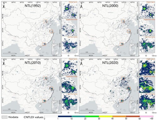
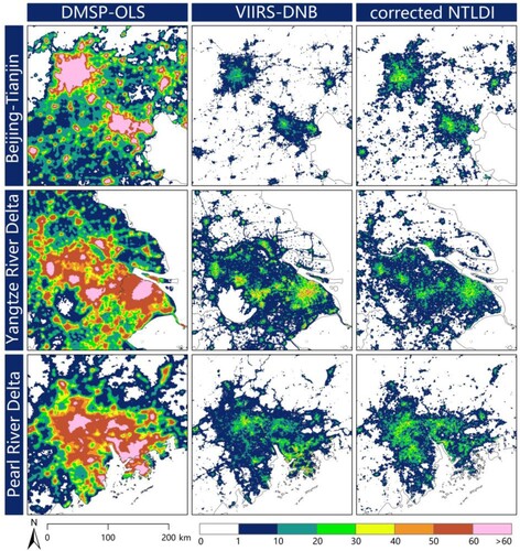
Figure 4. The details of DMSP-OLS, VIIRS-DNB, and CNTLDI data for the year 2012.

4.2 Population spatialization results

Taking the mean values of CNTLDI and ISAs at county level as independent variables and county-level population density as the dependent variable, we chose the GWR model to obtain the grid level population. Before implement the GWR test the multicollinearity among the predictors was considered. As the largest VIF in this study is 4.364, which is less than 10 (Table 3). Therefore, we don’t need to consider the multicollinearity problem.

Table 3. The tolerance and VIF of GWR in different years.

1990		2000		2010		2020
Tolerance	VIF	Tolerance	VIF	Tolerance	VIF	Tolerance	VIF
0.338	2.959	0.297	3.367	0.260	3.849	0.229	4.364

The $R^2$, adjusted $R^2$, and AICc are used as indicators to evaluate the accuracy of the fitting results. Table 4 summarizes the overall fitting effect of the GWR model. The values for adjusted $R^2$ are all higher than 0.8, the overall fitting effect is good, especially the results obtained based on CNTLDI variables (1990, 2000, and 2010), which are generally higher than those based on VIIRS-DNB (2020). The spatial diversity of local $R^2$ is shown in Figure 5. AICc is an information criterion that takes into account the complexity of the model, and the smaller of the value, the better of the model fitting. From Table 4, it can be seen that the 1990 model had the best fitting performance, and over time, the fitting performance deteriorated.

Figure 5. Local R² of the GWR model.

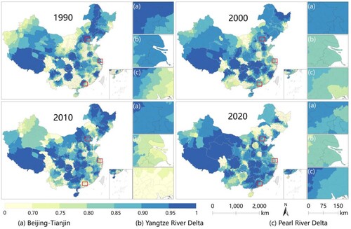
Table 4. Overall fitting accuracy of the GWR model.

Accuracy	1990	2000	2010	2020
R^2	0.92	0.92	0.89	0.86
Adjusted R^2	0.91	0.90	0.88	0.84
AICc	37590	37810	39511	41527

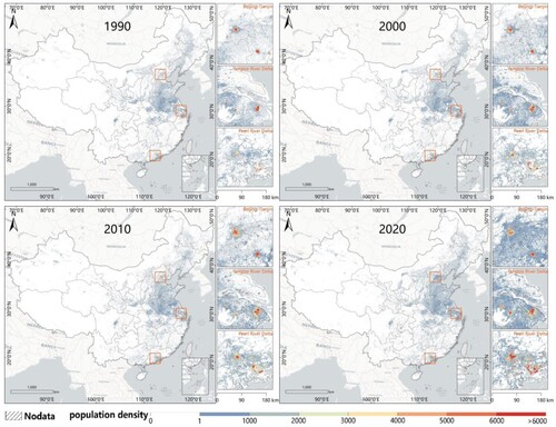
The model trained at the county level is used to obtain a preliminary grid-level population spatial distribution map with a spatial resolution of 500 m, and a population correction formula is used to modify the above preliminary results to obtain high-precision population distribution results for China in 1990, 2000, 2010, and 2020 (Figure 6). The results show that in China, the population density is relatively scattered in the west and concentrated in the east, presenting a multi-center spatial aggregation pattern. The Beijing–Tianjin–Hebei, Yellow River Basin, Sichuan Basin, Yangtze River Delta, and Pearl River Delta are the main densely populated areas. From 1990 to 2020, the scope of population distribution has gradually expanded, and the urban population has continued to increase, which demonstrates that the level of urbanization has accelerated.

Figure 6. Distribution of population density in China from 1990 to 2000 at 500 m resolution.

4.3 Spatiotemporal features of population density

It can be seen from Table 5 that the global Moran's I value is greater than 0.48, the Z value is greater than 43.25, and the P value is close to 0, which demonstrates that the population distribution in China has obvious positive autocorrelation. The local Moran’s I at prefecture level (as shown in Figure 7) and county level (as shown in Figure 8) were also calculated. The result is divided into five categories, including high–high (HH) cluster, high–low (HL) cluster, low–high (LH) cluster, low–low (LL) cluster, and no significant (NS). The changes in cluster patterns at the prefecture level and county level are basically consistent, and the correlation types of the population are dominated by HH and LL clusters. However, the distribution pattern of spatial autocorrelation types at different scales also differs in some local regions. For example, in Northeast China, there are many LL clusters at the county level, but there is no cluster at prefecture level. In Northwest China, there are some HL clusters at county level, but there are few such clusters at the prefecture level. This phenomenon is due to the influence of scale dependence and scale effect, and differences are observed in the space–time pattern characteristics of population distribution at different scales. In general, spatial dependence and heterogeneity can be more readily revealed at small rather than large spatial scales. From the county level scale, we can see a significant increase in the LL cluster while the HL cluster has continuously decreased in Northeast China, which indicates serious population loss in the most recent thirty years. The eastern and central regions of China have maintained HH clusters and stable spatial patterns at both the prefecture and county levels, indicating that the eastern and central regions have persistently remained highly attractive to the population, especially the southeast coastal areas. Although the population distribution of Sichuan Basin still has certain HH clusters, there is an obvious downward trend, which deserves further attention.

Figure 7. Local Moran’s I at prefecture level.

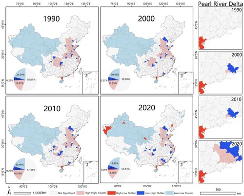
Figure 8. Local Moran’s I at county level.

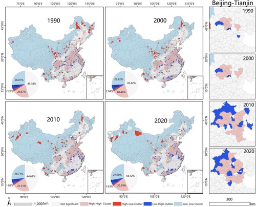
Table 5. The result of global Moran’s I.

Correlation indicators	1990	2000	2010	2020
Moran’s I	0.48	0.50	0.53	0.49
Z score	43.25	44.64	47.00	43.89
P value	<1*10^−3	<1*10^−3	<1*10^−3	<1*10^−3

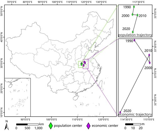
The change features of population density distribution can be seen from the movement of PCG. Here, the PCG in China is calculated for 1990, 2000, 2010, and 2020. The migration trajectory of the result is shown in Figure 9. From 1990 to 2000, the PCG shifted southward. From 2000 to 2010, the PCG shifted eastward. And from 2010 to 2020, the PCG continued to shift southward. At the same time, the economic center is also shown in the figure. By comparing the migration trajectory of the population center and the economic center, the movement trend of the two is relatively similar. It is confirmed that the economic situation is an important factor leading to population change. Therefore, this paper further studies the driving factors of population density change from various aspects related to economy.

Figure 9. Migration trajectory of population center of gravity and economic center of gravity.

4.4 Analysis of driving factors

To avoid estimation errors caused by multicollinearity between variables, we used the ridge regression model to study the impact of the value added of primary industry (AVPI), secondary industry (AVSI), and tertiary industry (AVTI) on population from 1990 to 2020. In order to pass the Multicollinearity test, it is necessary to ensure that the maximum value of VIF in each variable is less than 10. As shown in Table 6, the K values of ridge regression models in 1990, 2000, 2010, and 2020 were 0.01, 0.02, 0.02, and 0.01, respectively.

Table 6. The maximum value of VIF among variables of ridge regression.

K value	VIF
	1990	2000	2010	2020
0.00	12.480	23.585	16.631	11.684
0.01	8.668	11.934	10.272	8.143
0.02	6.393	7.263	6.997	6.022

As shown in Table 7, the R² of the model was above 0.9 in all years, and the model fits well. Based on the result of the F test, the ridge regression model can well describe the relationship between independent variables and dependent variable, optimize multicollinearity problem, and make the model more robust and explainable.According to the elastic coefficients and significance of influencing factors, it can be inferred that the value added of primary industry has a significant positive correlation with the population, but this influence strength is gradually weakening over time. By 2020, the value added of tertiary industry has a significant positive correlation with the population.

Table 7. Analysis result of ridge regression.

	1990	2000	2010	2020
Constant	0.071* (2.576)	0.072** (2.808)	0.046 (1.819)	−0.001 (−0.028)
AVPI	1.022*** (10.895)	0.920** (11.463)	0.720** (8.530)	0.468** (8.608)
AVSI	0.055 (0.377)	0.035 (0.222)	0.100 (0.660)	0.154 (1.124)
AVTI	−0.165 (−0.810)	−0.001 (−0.009)	0.244 (1.812)	0.345* (2.643)
R^2	0.915	0.922	0.917	0.934
Adjust-R^2	0.905	0.913	0.907	0.926
F value	96.367***	105.694***	98.885***	126.419***

Note: The numbers in parentheses are the t statistics.

*indicates significant at 10% confidence level.

**indicates significant at 5% confidence level.

***indicates significant at 1% confidence level.

5. Discussion

At present, NTL data are often used in large-scale and long time series socioeconomic-related studies. Although the DMSP-OLS dataset is widely used in population spatialization, its shortcomings are also obvious, such as serious saturation and overflow problems, lack of onboard calibration, and low spatial resolution. Since the emergence of VIIRS-DNB in 2012, this data has been used for various studies due to its high spatial resolution and non-saturation. However, its time series is still limited. There is an urgent need to integrated these two datasets to obtain a long time series of dataset for socio-economic research, especially for the research of population spatialization, the dataset can be used to provide rich information about population spatiotemporal changes. In this study, we adopted the NTLDI to alleviate the saturation problem of DMSP-OLS using NDVI data. The AE model was introduced to NTLDI, and the CNTLDI products with a spatial resolution of 500 m between 1992 and 2013 were then generated. The integration of use of CNTLDI and VIIRS-DNB can expand the time coverage of NTL data from 1992 to now. The existing population datasets such as LandScan and WorldPop provide data from 2000 with limited time series, while GHS-POP only utilizes land use data with limited accuracy. This study provides a new method for establishing spatialized population data in long time series.

The GWR model was used to simulate the relationship between county-level population density and county-level mean values of NTL and ISAs. The trained model was then used to generate a population spatial distribution map of China from 1990 to 2020 with 500 m resolution. Through spatial autocorrelation and PCG, we analyzed the features of China's population distribution change from 1990 to 2020, and found that the urban scope is constantly expanding, and the corresponding urban population is also increasing, especially in some major economic zones, such as the Beijing-Tianjin-Hebei, Yangtze River Delta, and Pearl River Delta. On the other hand, from the perspective of population spatialization, the population in Northeast China is gradually decreasing, which is probably to affect the local economic development.

Through analyzing the spatiotemporal characteristics of population distribution, the areas with high population density were found to be mainly concentrated in the eastern coastal areas of China, whereas the areas with low population distribution are mainly concentrated in western China. With the passage of time, the PCG moved from the north to the south of China. We also analyzed the driving factors of population distribution and found the value added of primary industry has a significant positive correlation with the population, but this influence strength is gradually weakening over time. The value added of tertiary industry has a positive correlation with the population by 2020, and this positive correlation is gradually increasing.

6. Conclusion

Our research still has some limitations. First, regarding the method used in this paper, good results have only been achieved in China. Second, the analysis of the driving factors of population distribution is not sufficiently comprehensive, given the impact of other economic and geographical factors was not considered. Last but not the least, the spatial distribution of population is influenced by various factors such as environment and economy, which exhibit diverse, complex, and heterogeneous spatial characteristics. The population distribution patterns revealed by different scales of population density data and their relationship with geographical environment are also different. Geographically weighted regression models neglect the modifiable areal unit problem (MAUP) when disaggregating population data. The training layer of the model is based on county-level census data, but the application layer uses 500 m resolution gridded units, resulting in significant changes in scale and alterations in the characteristics of population distribution. Due to insufficient characteristics of data, the prediction performance of the model is constrained for inferring from a state of poor population spatial distribution information to a state of complex population spatial distribution information. Scale determines the range and content of spatial data, and thus decides the extraction of information and representation of objectives. A change in scale will lead to a change in the conveyance of information. In future work, a deep understanding of the scale dependence of population distribution can be achieved by considering the geospatial mechanisms that constrain population distribution at different scales when building models. we will also need to consider the possibility of applying this method to population research in other parts of the world and consider additional driving factors that affect the spatial distribution of the population.

Population is often associated with multiple economic and social factors, the establishment of population spatialization datasets using multi-source data such as environmental, socio-economic, and demographic often helps to improve accuracy. We suggest that relevant information can be included in future research.

Disclosure statement

No potential conflict of interest was reported by the author(s).

Data availability statement

The data that support the findings of this study are available from the corresponding author upon reasonable request.

Additional information

Funding

This work was supported by National Natural Science Foundation of China [Grant Number 41930650]; Ningxia Hui Autonomous Region Key Research and Development Project [Grant Number 2022BEG03064]; State Key Laboratory of Geo-Information Engineering and Key Laboratory of Surveying and Mapping Science and Geospatial Information Technology of MNR, CASM [Grant Number 2021-03-04].

References

- Alahmadi, Mohammed, Shawky Mansour, Nataraj Dasgupta, Ammar Abulibdeh, Peter M Atkinson, and David J Martin. 2021a. “Using Daily Nighttime Lights to Monitor Spatiotemporal Patterns of Human Lifestyle Under Covid-19: The Case of Saudi Arabia.” Remote Sensing 13 (22): 4633. https://doi.org/10.3390/rs13224633.
- Alahmadi, Mohammed, Shawky Mansour, Nataraj Dasgupta, and David J Martin. 2023. “Using Nighttime Lights Data to Assess the Resumption of Religious and Socioeconomic Activities Post-COVID-19.” Remote Sensing 15 (4): 1064. https://doi.org/10.3390/rs15041064.
- Alahmadi, Mohammed, Shawky Mansour, David Martin, and Peter M Atkinson. 2021b. “An Improved Index for Urban Population Distribution Mapping Based on Nighttime Lights (DMSP-OLS) Data: An Experiment in Riyadh Province, Saudi Arabia.” Remote Sensing 13 (6): 1171. https://doi.org/10.3390/rs13061171.
- Amaral, Silvana, Antonio MV Monteiro, Gilberto Câmara, and José Alberto Quintanilha. 2006. “DMSP/OLS Night-Time Light Imagery for Urban Population Estimates in the Brazilian Amazon.” International Journal of Remote Sensing 27 (05): 855–870. https://doi.org/10.1080/01431160500181861.
- Assuncao, Renato M, and Edna A Reis. 1999. “A new Proposal to Adjust Moran'sI for Population Density.” Statistics in Medicine 18 (16): 2147–2162. https://doi.org/10.1002/(SICI)1097-0258(19990830)18:163.0.CO;2-I.
- Azar, Derek, Ryan Engstrom, Jordan Graesser, and Joshua Comenetz. 2013. “Generation of Fine-Scale Population Layers Using Multi-Resolution Satellite Imagery and Geospatial Data.” Remote Sensing of Environment 130: 219–232. https://doi.org/10.1016/j.rse.2012.11.022.
- Chen, Zuoqi, Bailang Yu, Chengshu Yang, Yuyu Zhou, Shenjun Yao, Xingjian Qian, Congxiao Wang, Bin Wu, and Jianping Wu. 2021. “An Extended Time Series (2000–2018) of Global NPP-VIIRS-Like Nighttime Light Data from a Cross-Sensor Calibration.” Earth System Science Data 13 (3): 889–906. https://doi.org/10.5194/essd-13-889-2021.
- Cheng, Zhifeng, Jianghao Wang, and Yong Ge. 2022. “Mapping Monthly Population Distribution and Variation at 1-km Resolution Across China.” International Journal of Geographical Information Science 36 (6): 1166–1184. https://doi.org/10.1080/13658816.2020.1854767.
- Chu, Hone-Jay, Chen-Han Yang, and Chelsea C Chou. 2019. “Adaptive non-Negative Geographically Weighted Regression for Population Density Estimation Based on Nighttime Light.” ISPRS International Journal of Geo-Information 8 (1): 26. https://doi.org/10.3390/ijgi8010026.
- Daniele, Ehrlich, Balk Deborah, and Richard Sliuzas. 2020. “Measuring and understanding global human settlements patterns and processes: Innovation, progress and application.” International journal of digital earth 13 (1): 2–8. https://doi.org/10.1080/17538947.2019.1630072.
- Elvidge, Christopher D, Kimberly E Baugh, John B Dietz, Theodore Bland, Paul C Sutton, and Herbert W Kroehl. 1999. “Radiance Calibration of DMSP-OLS low-Light Imaging Data of Human Settlements.” Remote Sensing of Environment 68 (1): 77–88. https://doi.org/10.1016/S0034-4257(98)00098-4.
- Elvidge, Christopher D, Kimberly E Baugh, Mikhail Zhizhin, and Feng-Chi Hsu. 2013a. “Why VIIRS Data are Superior to DMSP for Mapping Nighttime Lights.” Proceedings of the Asia-Pacific Advanced Network 35 (0): 62. https://doi.org/10.7125/APAN.35.7.
- Elvidge, Christopher D, Mikhail Zhizhin, Feng-Chi Hsu, and Kimberly E Baugh. 2013b. “VIIRS Nightfire: Satellite Pyrometry at Night.” Remote Sensing 5 (9): 4423–4449. https://doi.org/10.3390/rs5094423.
- Elvidge, Christopher D, Mikhail Zhizhin, David Keith, Steven D Miller, Feng Chi Hsu, Tilottama Ghosh, Sharolyn J Anderson, Christian K Monrad, Morgan Bazilian, and Jay Taneja. 2022. “The VIIRS Day/Night Band: A Flicker Meter in Space?” Remote Sensing 14 (6): 1316. https://doi.org/10.3390/rs14061316.
- Gaughan, Andrea E, Forrest R Stevens, Zhuojie Huang, Jeremiah J Nieves, Alessandro Sorichetta, Shengjie Lai, Xinyue Ye, Catherine Linard, Graeme M Hornby, and Simon I Hay. 2016. “Spatiotemporal Patterns of Population in Mainland China, 1990 to 2010.” Scientific Data 3 (1): 1–11. https://doi.org/10.1038/sdata.2016.5.
- Guo, Wei, Yongxing Li, Peixian Li, Xuesheng Zhao, and Jinyu Zhang. 2022. “Using a Combination of Nighttime Light and MODIS Data to Estimate Spatiotemporal Patterns of CO2 Emissions at Multiple Scales.” Science of The Total Environment 848: 157630. https://doi.org/10.1016/j.scitotenv.2022.157630.
- Guo, Wei, Guiying Li, Wenjian Ni, Yuhuan Zhang, and Dengsheng Lu. 2018a. “Exploring Improvement of Impervious Surface Estimation at National Scale Through Integration of Nighttime Light and Proba-v Data.” GIScience & Remote Sensing 55 (5): 699–717. https://doi.org/10.1080/15481603.2018.1436425.
- Guo, Wei, Dengsheng Lu, and Wenhui Kuang. 2017. “Improving Fractional Impervious Surface Mapping Performance Through Combination of DMSP-OLS and MODIS NDVI Data.” Remote Sensing 9 (4): 375. https://doi.org/10.3390/rs9040375.
- Guo, Wei, Dengsheng Lu, Yanlan Wu, and Jixian Zhang. 2015. “Mapping Impervious Surface Distribution with Integration of SNNP VIIRS-DNB and MODIS NDVI Data.” Remote Sensing 7 (9): 12459–12477. https://doi.org/10.3390/rs70912459.
- Guo, Wei, Yuhuan Zhang, and Le Gao. 2018. “Using VIIRS-DNB and Landsat Data for Impervious Surface Area Mapping in an Arid/Semiarid Region.” Remote Sensing Letters 9 (6): 587–596. https://doi.org/10.1080/2150704X.2018.1455234.
- Guo, Wei, Jinyu Zhang, Xuesheng Zhao, Yongxing Li, Jinke Liu, Wenbin Sun, and Deqin Fan. 2023. “Combining Luojia1-01 Nighttime Light and Points-of-Interest Data for Fine Mapping of Population Spatialization Based on The Zonal Classification Method.” IEEE Journal of Selected Topics in Applied Earth Observations and Remote Sensing 16:1589–1600. https://doi.org/10.1109/JSTARS.2023.3238188.
- Harvey, J. T. 2002. “Estimating Census District Populations from Satellite Imagery: Some Approaches and Limitations.” International Journal of Remote Sensing 23 (10): 2071–2095. https://doi.org/10.1080/01431160110075901.
- Hu, Maogui, Zhongjie Li, Jinfeng Wang, Lin Jia, Yilan Liao, Shengjie Lai, Yansha Guo, Dan Zhao, and Weizhong Yang. 2012. “Determinants of the Incidence of Hand, Foot and Mouth Disease in China Using Geographically Weighted Regression Models.” PloS one 7 (6): e38978. https://doi.org/10.1371/journal.pone.0038978.
- Huang, Xiao, Cuizhen Wang, Zhenlong Li, and Huan Ning. 2021. “A 100 m Population Grid in the CONUS by Disaggregating Census Data with Open-Source Microsoft Building Footprints.” Big Earth Data 5 (1): 112–133. https://doi.org/10.1080/20964471.2020.1776200.
- Huang, Qingxu, Xi Yang, Bin Gao, Yang Yang, and Yuanyuan Zhao. 2014. “Application of DMSP/OLS Nighttime Light Images: A Meta-Analysis and a Systematic Literature Review.” Remote Sensing 6 (8): 6844–6866. https://doi.org/10.3390/rs6086844.
- Huang, Qingxu, Yang Yang, Yajing Li, and Bin Gao. 2016. “A Simulation Study on the Urban Population of China Based on Nighttime Light Data Acquired from DMSP/OLS.” Sustainability 8 (6): 521. https://doi.org/10.3390/su8060521.
- Huang, Yaohuan, Chuanpeng Zhao, Xiaoyang Song, Jie Chen, and Zhonghua Li. 2018. “A Semi-Parametric Geographically Weighted (S-GWR) Approach for Modeling Spatial Distribution of Population.” Ecological Indicators 85: 1022–1029. https://doi.org/10.1016/j.ecolind.2017.11.028.
- Jing, Wenlong, Yaping Yang, Xiafang Yue, and Xiaodan Zhao. 2015. “Mapping Urban Areas with Integration of DMSP/OLS Nighttime Light and MODIS Data Using Machine Learning Techniques.” Remote Sensing 7 (9): 12419–12439. https://doi.org/10.3390/rs70912419.
- Letu, Husi, Masanao Hara, Gegen Tana, and Fumihiko Nishio. 2012. “A Saturated Light Correction Method for DMSP/OLS Nighttime Satellite Imagery.” IEEE Transactions on Geoscience and Remote Sensing 50 (2): 389–396. https://doi.org/10.1109/TGRS.2011.2178031.
- Levin, Noam, Christopher CM Kyba, Qingling Zhang, Alejandro Sánchez de Miguel, Miguel O Román, Xi Li, Boris A Portnov, Andrew L Molthan, Andreas Jechow, and Steven D Miller. 2020. “Remote Sensing of Night Lights: A Review and an Outlook for the Future.” Remote Sensing of Environment 237: 111443. https://doi.org/10.1016/j.rse.2019.111443.
- Levin, Noam, and Qingling Zhang. 2017. “A Global Analysis of Factors Controlling VIIRS Nighttime Light Levels from Densely Populated Areas.” Remote Sensing of Environment 190: 366–382. https://doi.org/10.1016/j.rse.2017.01.006.
- Leyk, Stefan, Andrea E Gaughan, Susana B Adamo, Alex de Sherbinin, Deborah Balk, Sergio Freire, Amy Rose, Forrest R Stevens, Brian Blankespoor, and Charlie Frye. 2019. “The Spatial Allocation of Population: A Review of Large-Scale Gridded Population Data Products and Their Fitness for use.” Earth System Science Data 11 (3): 1385–1409. https://doi.org/10.5194/essd-11-1385-2019.
- Li, Xuecao, and Yuyu Zhou. 2017. “A Stepwise Calibration of Global DMSP/OLS Stable Nighttime Light Data (1992–2013).” Remote Sensing 9 (6): 637. https://doi.org/10.3390/rs9060637.
- Li, Xiaoma, and Weiqi Zhou. 2018. “Dasymetric Mapping of Urban Population in China Based on Radiance Corrected DMSP-OLS Nighttime Light and Land Cover Data.” Science of The Total Environment 643: 1248–1256. https://doi.org/10.1016/j.scitotenv.2018.06.244.
- Liang, Longwu, Mingxing Chen, Xinyue Luo, and Yue Xian. 2021. “Changes Pattern in the Population and Economic Gravity Centers Since the Reform and Opening up in China: The Widening Gaps Between the South and North.” Journal of Cleaner Production 310: 127379. https://doi.org/10.1016/j.jclepro.2021.127379.
- Linard, Catherine, Victor A Alegana, Abdisalan M Noor, Robert W Snow, and Andrew J Tatem. 2010. “Enhancing Spatial Detection Accuracy for Syndromic Surveillance with Street Level Incidence Data.” International Journal of Health Geographics 9 (1): 1–13. https://doi.org/10.1186/1476-072X-9-1.
- Linard, Catherine, and Andrew J Tatem. 2012. “Neighborhood Level Risk Factors for Type 1 Diabetes in Youth: The SEARCH Case-Control Study.” International Journal of Health Geographics 11: 1–13. https://doi.org/10.1186/1476-072X-11-1.
- Liu, Zhifeng, Chunyang He, Qiaofeng Zhang, Qingxu Huang, and Yang Yang. 2012. “Extracting the Dynamics of Urban Expansion in China Using DMSP-OLS Nighttime Light Data from 1992 to 2008.” Landscape and Urban Planning 106 (1): 62–72. https://doi.org/10.1016/j.landurbplan.2012.02.013.
- Liu, Jiyuan, Wenhui Kuang, Zengxiang Zhang, Xinliang Xu, Yuanwei Qin, Jia Ning, Wancun Zhou, Shuwen Zhang, Rendong Li, and Changzhen Yan. 2014. “Spatiotemporal Characteristics, Patterns, and Causes of Land-use Changes in China Since the Late 1980s.” Journal of Geographical Sciences 24: 195–210. https://doi.org/10.1007/s11442-014-1082-6.
- Lu, Dengsheng, Hanqin Tian, Guomo Zhou, and Hongli Ge. 2008. “Regional Mapping of Human Settlements in Southeastern China with Multisensor Remotely Sensed Data.” Remote Sensing of Environment 112 (9): 3668–3679. https://doi.org/10.1016/j.rse.2008.05.009.
- Lu, Dan, Yahui Wang, Qingyuan Yang, Kangchuan Su, Haozhe Zhang, and Yuanqing Li. 2021. “Modeling Spatiotemporal Population Changes by Integrating DMSP-OLS and NPP-VIIRS Nighttime Light Data in Chongqing, China.” Remote Sensing 13 (2): 284. https://doi.org/10.3390/rs13020284.
- Lv, Qian, Haibin Liu, Jingtao Wang, Hao Liu, and Yu Shang. 2020. “Multiscale Analysis on Spatiotemporal Dynamics of Energy Consumption CO2 Emissions in China: Utilizing the Integrated of DMSP-OLS and NPP-VIIRS Nighttime Light Datasets.” Science of The Total Environment 703: 134394. https://doi.org/10.1016/j.scitotenv.2019.134394.
- Ma, Ting, Chenghu Zhou, Tao Pei, Susan Haynie, and Junfu Fan. 2014. “Responses of Suomi-NPP VIIRS-Derived Nighttime Lights to Socioeconomic Activity in China’s Cities.” Remote Sensing Letters 5 (2): 165–174. https://doi.org/10.1080/2150704X.2014.890758.
- Miller, Steven D, Stephen P Mills, Christopher D Elvidge, Daniel T Lindsey, Thomas F Lee, and Jeffrey D Hawkins. 2012. “Suomi Satellite Brings to Light a Unique Frontier of Nighttime Environmental Sensing Capabilities.” Proceedings of the National Academy of Sciences 109 (39): 15706–15711. https://doi.org/10.1073/pnas.1207034109.
- O’brien, Robert. 2007. “A Caution Regarding Rules of Thumb for Variance Inflation Factors.” Quality & Quantity 41: 673–690. https://doi.org/10.1007/s11135-006-9018-6.
- Qiu, Yue, Xuesheng Zhao, Deqin Fan, Songnian Li, and Yijing Zhao. 2022. “Disaggregating Population Data for Assessing Progress of SDGs: Methods and Applications.” International Journal of Digital Earth 15 (1): 2–29. https://doi.org/10.1080/17538947.2021.2013553.
- Shang, Shuoshuo, Shihong Du, Shouji Du, and Shoujie Zhu. 2021. “Estimating Building-Scale Population Using Multi-Source Spatial Data.” Cities 111: 103002. https://doi.org/10.1016/j.cities.2020.103002.
- Shi, Kaifang, Bailang Yu, Yixiu Huang, Yingjie Hu, Bing Yin, Zuoqi Chen, Liujia Chen, and Jianping Wu. 2014. “Evaluating the Ability of NPP-VIIRS Nighttime Light Data to Estimate the Gross Domestic Product and the Electric Power Consumption of China at Multiple Scales: A Comparison with DMSP-OLS Data.” Remote Sensing 6 (2): 1705–1724. https://doi.org/10.3390/rs6021705.
- Stevens, Forrest R, Andrea E Gaughan, Jeremiah J Nieves, Adam King, Alessandro Sorichetta, Catherine Linard, and Andrew J Tatem. 2020. “Comparisons of two Global Built Area Land Cover Datasets in Methods to Disaggregate Human Population in Eleven Countries from the Global South.” International Journal of Digital Earth 13 (1): 78–100. https://doi.org/10.1080/17538947.2019.1633424.
- Sun, Weichao, Xia Zhang, Nan Wang, and Yi Cen. 2017. “Estimating Population Density Using DMSP-OLS Night-Time Imagery and Land Cover Data.” IEEE Journal of Selected Topics in Applied Earth Observations and Remote Sensing 10 (6): 2674–2684. https://doi.org/10.1109/JSTARS.2017.2703878.
- Sutton, Paul, Dar Roberts, Christopher Elvidge, and Kimberly Baugh. 2001. “Census from Heaven: An Estimate of the Global Human Population Using Night-Time Satellite Imagery.” International Journal of Remote Sensing 22 (16): 3061–3076. https://doi.org/10.1080/01431160010007015.
- Sutton, Paul, Dar Roberts, Chris Elvidge, and Henk Meij. 1997. “A Comparison of Nighttime Satellite Imagery.” Photogrammetric Engineering & Remote Sensing 63 (11): 1303–1313. 0099-1112/97/6311-1303$3.00/0.
- Wang, Shaojian, Chuanglin Fang, Haitao Ma, Yang Wang, and Jing Qin. 2014. “Spatial Differences and Multi-Mechanism of Carbon Footprint Based on GWR Model in Provincial China.” Journal of Geographical Sciences 24: 612–630. https://doi.org/10.1007/s11442-014-1109-z.
- Wang, Litao, Shixin Wang, Yi Zhou, Wenliang Liu, Yanfang Hou, Jinfeng Zhu, and Futao Wang. 2018. “Mapping Population Density in China Between 1990 and 2010 Using Remote Sensing.” Remote Sensing of Environment 210: 269–281. https://doi.org/10.1016/j.rse.2018.03.007.
- Wardrop, N. A., W. C. Jochem, T. J. Bird, H. R. Chamberlain, Donna Clarke, David Kerr, Linus Bengtsson, Sabrina Juran, Vincent Seaman, and A. J. Tatem. 2018. “Spatially Disaggregated Population Estimates in the Absence of National Population and Housing Census Data.” Proceedings of the National Academy of Sciences 115 (14): 3529–3537. https://doi.org/10.1073/pnas.1715305115.
- Wu, Yizhen, Kaifang Shi, Zuoqi Chen, Shirao Liu, and Zhijian Chang. 2021. “Developing Improved Time-Series DMSP-OLS-Like Data (1992–2019) in China by Integrating DMSP-OLS and SNPP-VIIRS.” IEEE Transactions on Geoscience and Remote Sensing 60: 1–14. https://doi.org/10.1109/TGRS.2021.3135333.
- Xiong, Junnan, Kun Li, Weiming Cheng, Chongchong Ye, and Hao Zhang. 2019. “A Method of Population Spatialization Considering Parametric Spatial Stationarity: Case Study of the Southwestern Area of China.” ISPRS International Journal of Geo-Information 8 (11): 495. https://doi.org/10.3390/ijgi8110495.
- Ye, Tingting, Naizhuo Zhao, Xuchao Yang, Zutao Ouyang, Xiaoping Liu, Qian Chen, Kejia Hu, Wenze Yue, Jiaguo Qi, and Zhansheng Li. 2019. “Improved Population Mapping for China Using Remotely Sensed and Points-of-Interest Data Within a Random Forests Model.” Science of The Total Environment 658: 936–946. https://doi.org/10.1016/j.scitotenv.2018.12.276.
- Yong, Zhiwei, Kun Li, Junnan Xiong, Weiming Cheng, Zegen Wang, Huaizhang Sun, and Chongchong Ye. 2022. “Integrating DMSP-OLS and NPP-VIIRS Nighttime Light Data to Evaluate Poverty in Southwestern China.” Remote Sensing 14 (3): 600. https://doi.org/10.3390/rs14030600.
- Yuan, Xiaotian, Li Jia, Massimo Menenti, and Min Jiang. 2022. “Consistent Nighttime Light Time Series in 1992–2020 in Northern Africa by Combining DMSP-OLS and NPP-VIIRS Data.” Big Earth Data 6 (4): 603–632. https://doi.org/10.1080/20964471.2022.2031542.
- Zhang, Qingling, Bhartendu Pandey, and Karen C Seto. 2016. “A Robust Method to Generate a Consistent Time Series from DMSP/OLS Nighttime Light Data.” IEEE Transactions on Geoscience and Remote Sensing 54 (10): 5821–5831. https://doi.org/10.1109/TGRS.2016.2572724.
- Zhang, Qian, Juqin Shen, and Fuhua Sun. 2021. “Spatiotemporal Differentiation of Coupling Coordination Degree Between Economic Development and Water Environment and its Influencing Factors Using GWR in China's Province.” Ecological Modelling 462: 109794. https://doi.org/10.1016/j.ecolmodel.2021.109794.
- Zhang, Zengxiang, Xiao Wang, Xiaoli Zhao, Bin Liu, Lin Yi, Lijun Zuo, Qingke Wen, Fang Liu, Jinyong Xu, and Shunguang Hu. 2014. “A 2010 Update of National Land Use/Cover Database of China at 1:100000 Scale Using Medium Spatial Resolution Satellite Images.” Remote Sensing of Environment 149: 142–154. https://doi.org/10.1016/j.rse.2014.04.004.
- Zhao, Jincai, Guangxing Ji, YanLin Yue, Zhizhu Lai, Yulong Chen, Dongyang Yang, Xu Yang, and Zheng Wang. 2019. “Spatio-temporal Dynamics of Urban Residential CO2 Emissions and Their Driving Forces in China Using the Integrated two Nighttime Light Datasets.” Applied Energy 235: 612–624. https://doi.org/10.1016/j.apenergy.2018.09.180.
- Zhao, Song, Yanxu Liu, Rui Zhang, and Bojie Fu. 2020a. “China’s Population Spatialization Based on Three Machine Learning Models.” Journal of Cleaner Production 256: 120644. https://doi.org/10.1016/j.jclepro.2020.120644.
- Zhao, Min, Yuyu Zhou, Xuecao Li, Chenghu Zhou, Weiming Cheng, Manchun Li, and Kun Huang. 2020b. “Building a Series of Consistent Night-Time Light Data (1992–2018) in Southeast Asia by Integrating DMSP-OLS and NPP-VIIRS.” IEEE Transactions on Geoscience and Remote Sensing 58 (3): 1843–1856. https://doi.org/10.1109/TGRS.2019.2949797.
- Zheng, Qiming, Qihao Weng, and Ke Wang. 2019. “Developing a new Cross-Sensor Calibration Model for DMSP-OLS and Suomi-NPP VIIRS Night-Light Imageries.” ISPRS Journal of Photogrammetry and Remote Sensing 153: 36–47. https://doi.org/10.1016/j.isprsjprs.2019.04.019.
- Zhou, Yuyu, Steven J Smith, Christopher D Elvidge, Kaiguang Zhao, Allison Thomson, and Marc Imhoff. 2014. “A Cluster-Based Method to map Urban Area from DMSP/OLS Nightlights.” Remote Sensing of Environment 147: 173–185. https://doi.org/10.1016/j.rse.2014.03.004.
- Zhou, Qianling, Changxin Wang, and Shijiao Fang. 2019. “Application of Geographically Weighted Regression (GWR) in the Analysis of the Cause of Haze Pollution in China.” Atmospheric Pollution Research 10 (3): 835–846. https://doi.org/10.1016/j.apr.2018.12.012.
- Zhuo, Li, Toshiaki Ichinose, Junyuan Zheng, Jin Chen, Peijun Shi, and X. Li. 2009. “Modelling the Population Density of China at the Pixel Level Based on DMSP/OLS non-Radiance-Calibrated Night-Time Light Images.” International Journal of Remote Sensing 30 (4): 1003–1018. https://doi.org/10.1080/01431160802430693.
- Zhuo, Li, Jing Zheng, Xiaofan Zhang, Jun Li, and Lin Liu. 2015. “An Improved Method of Night-Time Light Saturation Reduction Based on EVI.” International Journal of Remote Sensing 36 (16): 4114–4130. https://doi.org/10.1080/01431161.2015.1073861.