Future variation of land surface temperature in the Yangtze River Basin based on CMIP6 model

ABSTRACT

In recent years, past changes in global and regional land surface temperatures (LST) have been well studied, however, future LST changes have been largely ignored owing to data limitations. In this study, three climate variables of CMIP6, namely air temperature (AT), precipitation (Pre), and leaf area index (LAI), were spatially corrected using the Delta downscaling method. On this basis, by combining MODIS LST, elevation, slope and aspect, a random forest (RF) model was built to calculate the LST from 2022 to 2100. The absolute variability (AV) and Mann-Kendall (M-K) tests were used to quantitatively detect interannual and seasonal LST changes in different Shared Socioeconomic Pathways (SSPs) scenarios. The results showed that the AV value increased successively from SSP1-2.6 to SSP2-4.5 and then to SSP5-8.5. Compared with the base period (2003-2021), the increment in interannual, spring, summer and autumn LST during 2022–2100 was mainly between 1 and 2 °C under three scenarios. The interannual and seasonal LST were spatially characterized by significant warming over large areas, and the increasing was the fastest under SSP5-8.5. These results indicate that, in the future, LST will increase further over large areas, especially in winter.

KEYWORDS:

• Temporal and spatial changes
• Delta downscaling
• Random forest
• Global warming

1. Introduction

Land surface temperature (LST) is a vital index for measuring the global environment, and has a positive response to climate change. LST variations directly affected the global net radiation balance and thus had a significant impact on the material and energy cycles, ecosystem stability, and sustainable development of human society (Mao et al. 2020). The Sixth Assessment Report of the Intergovernmental Panel on Climate Change (IPCC6) indicated that the global average temperature had increased by approximately 1 °C from 1850 to 1900, and the temperature in 2001–2020 was 0.99 °C higher than that in 1850–1900 (Masson-Delmotte et al. 2021). Under the background of global warming, the LST in East China, North China, Sichuan Basin and Tibetan Plateau all showed varying degrees of increase (Song et al. 2021). Among them, the LST in the Yangtze River Basin (YRB) increased by 0.36 °C in the past 19 years, and that in urban areas increased by 1.9–3.8 °C (Liu et al. 2022). The occurrence of urban heat would cause severe environmental, economic and social impacts (He et al. 2023). If mitigation strategies were not developed, then LST may increase further in the future.

Previous studies had shown that LST changes in different regions of the world exhibited similar patterns. Specifically, the annual mean LST experienced varying degrees of increase and a warming gap existed. For example, there were two turning points in 2007 and 2012 for LST in the agricultural pastural ecotone of northern China and the YRB, which were the same as the turning points in China (Wei et al. 2021; Liu et al. 2022). Asymmetric warming occurred during daytime and nighttime or seasonal LST. The specific manifestation was that the warming rate and warming area at nighttime in China were greater than those during the daytime, and the LST increased in almost all seasons except during the daytime in autumn (Song et al. 2021). In some areas, the warming area during the daytime was greater than that at nighttime, such as in the temperate zone of China (Du et al. 2019). Although historical LST changes had been well-documented in many studies, future LST changes were more important for the development of climate mitigation strategies. However, future changes were largely ignored because of imperfect forecasting methods or a lack of data. LST prediction methods were mainly divided into univariate-based and multivariate-based predictions (Bartkowiak, Castelli, and Notarnicola 2019; Jia et al. 2021). The most commonly used methods were time-series analysis, multiple linear regression and machine learning (Zafra, Ángel, and Torres 2017; Schwingshackl, Hirschi, and Seneviratne 2018; Feng et al. 2022). The autoregressive integrated moving average model (ARIMA) of time-series analysis had been identified as one of the most effective means of climate change prediction (Tang et al. 2022). Its prediction depended only on the time dependence of LST regularity. However, if the predictive variables were unstable, ARIMA failed to capture regularity, which made it difficult to predict an accurate LST (Zafra, Ángel, and Torres 2017). Multiple linear regression, the other proposed method, did not require LST to satisfy a specific regularity, but only required a strong linear relationship between multiple variables and LST (Schwingshackl, Hirschi, and Seneviratne 2018). However, the cross-effect among independent variables and the nonlinear relationship between independent variables and LST often affected the prediction accuracy of LST (Mohammad and Goswami 2021). With the development of machine learning, the nonlinear relationship between the independent variables and LST had been solved (Jia et al. 2021). The random forest (RF) model, which had the advantages of strong generalization ability and insensitivity to multicollinearity, was suitable for capturing nonlinear relations between variables (Xiao et al. 2021). Although the simplicity and efficiency of the RF model had led to its widespread use in LST reconstruction and downscaling research, if there was a lack of future data, the RF model could only predict historical data that had already occurred (Bartkowiak, Castelli, and Notarnicola 2019). Therefore, obtaining future data was key to solving long-term LST forecasts in the future.

Global climate models (GCMs) provided long-term climate information worldwide. Many studies had evaluated Phase 6 of the International Coupled Model Intercomparison Project (CMIP6) on a global or regional scale and found that the CMIP6 model could effectively predict future air temperature (AT), precipitation (Pre), and leaf area index (LAI) (Peng et al. 2017; You et al. 2021; Zhang et al. 2022; Sun, Xue, and Zhou 2023). Compared with the CMIP5 model, the CMIP6 model included multiple Shared Socioeconomic Pathways (SSPs) and more air pollutant emission scenarios, which could provide more reasonable data for regional climate research (Tokarska et al. 2020; Huang, Li, and Song 2022; Wang et al. 2023). The coarse resolution of the CMIP6 model (less than 100 km) could not accurately represent the climate of the complex terrain in the small-scale and medium-scale regions, therefore, spatial downscaling of the CMIP6 model data was the premise of future climate change research. Statistical downscaling, such as regression and Delta downscaling, was a widely used spatial downscaling method (Peng et al. 2017; Shui et al. 2019). Among them, the linear regression method was used to establish a linear relationship between the GCMs historical period data and the site observation data, and it was applied to the future period (Li et al. 2012; Timm, Giambelluca, and Diaz 2015). However, this method could not adequately describe the spatial distribution in areas with sparse sites, such as the Qinghai-Tibet Plateau, so could not construct high-resolution future climate datasets (Zhou et al. 2022). Previous studies had shown that using low spatial resolution data and high spatial resolution reference climate data as input data for Delta downscaling was very suitable for climate data downscaling (Peng et al. 2019). The basic idea of the Delta downscaling method consisted of assuming that the deviation of the historical period with respect to the reference period was still applicable in the future. Compared with direct interpolation, this process introduced the influence of topography on climate (Peng et al. 2017). Topographic effects were mainly derived from selected reference data. The WorldClim climate data, based on interpolations from 9000–60,000 weather stations around the world, took into account latitude, longitude, elevation, distance to the nearest coast, and three satellite-derived covariates obtained by the MODIS satellite platform: maximum and minimum LST and cloud cover. This reference data yielded high quality downscaling data by combining Delta downscaling method (Ding and Peng 2021). In general, the Delta downscaling method had obvious advantages for obtaining accurate climate data at small scales.

Although the CMIP6 model data provided convenience for the study of future climate change, the climate variables involved in the CMIP6 model did not include LST. Previous studies had shown that changes in LST were closely related to AT, Pre, vegetation, and topography (Song et al. 2021; Xiao et al. 2021). Based on this, future LST variations could be predicted using these variables combined with the RF model. Therefore, the main objectives of this study were to: (1) use the Delta downscaling method to generate high-resolution AT, Pre, and LAI of the YRB during 2003–2014 and 2022–2100, (2) use the RF model to establish the relationship between variables and LST and thus prediction LST from 2003 to 2014, and apply it to the future to generate LST data from 2022 to 2100; and (3) analyze temporal, spatial and trend changes of LST in the YRB during 2022–2100.

2. Material and methods

2.1. Study area

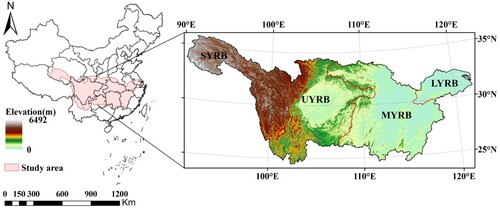
The Yangtze River Basin (YRB) originates in the hinterland of the Qinghai-Tibet Plateau and is the largest river in China, with a total area of 1.8 × 10⁶ km² and a total length of 6397 km, involving mountains, plateaus, basins, hills and plains (Figure 1). The mainstream of the YRB flows through 19 provinces, cities and autonomous regions. The upper reach of the YRB (UYRB) is from the source of the YRB (SYRB) to Yichang City, the middle reach of the YRB (MYRB) is from Yichang City to Hukou City, and the lower reach of the YRB (LYRB) is from Hukou City to the YRB Estuary. In recent decades, the YRB experienced rapid urbanization, and large urban agglomerations had been formed, such as Chengdu-Chongqing, the middle reaches of the YRB and the Yangtze River Delta. There are many climatic types in the YRB, including plateau mountain, southwest tropical monsoon and subtropical monsoon regions. The annual average rainfall in the YRB is approximately 1100 mm, which is mainly concentrated during the rainy season, accounting for 70%–90% of the annual rainfall. The annual average temperature of the YRB is characterized by diurnal asymmetrical variation. As an important ecological civilization construction base, the YRB, which accounts for 25%, 40% and 60% of the country’s cultivated land area, grain output and fish output, respectively, may be more susceptible to the impact of climate change (Yu et al. 2023).

Figure 1. The location of the YRB in China and the elevation of the YRB.

2.2. Data sources

The Aqua MYD11A2 LST product for 2003–2021 (V6.1), with 1-km spatial resolution and 8-day temporal resolution, was used to train and test the RF model. Overpass times of Aqua satellite was close to the times of the daily maximum and minimum. Good quality data were extracted from quality control documents, and outliers were eliminated using the Hampel filtering method.

Month AT, Pre and LAI data for the CMIP6 models were obtained from the CMIP6 archives. According to previous studies, we chose SSP1-2.6, SSP2-4.5 and SSP5-8.5 represented different radiative forcings (Zhu, Jiang, and Li 2021). SSP1-2.6 referred to sustainable development. SSP2-4.5 referred to that socio-economic factors follow the historical trend and do not change significantly. SSP5-8.5 referred to fossil fuel development, and the global economy was growing rapidly. The resolutions and agencies/countries of the five models selected in this study were listed in Table 1.

Table 1. The resolution and agencies/country of five models selected in the study.

Model	Resolution(km)	Country
EC-Earth3-veg	512*256	EC-Earth-Consortium/Europe
GFDL-ESM4	288*180	NOAA-GFDL/United States
BBC-CSM2-MR	320*160	BCC/China
EC-Earth3	512*256	EC-Earth-Consortium/Europe
MRI-ESM2-0	320*160	MRI/Japan

The high-resolution AT and Pre datasets were presented as grid data with a 1-km resolution (approximately 30’’) provided by WorldClim. The datasets were used as high-resolution reference data for spatial downscaling of AT and Pre. The WorldClim data generated based on weather stations worldwide using a thin-plate spline interpolation method and reflected topographic effects and climate information. Cross-validation correlations indicated that these reference data exhibited good performance globally (Ding and Peng 2021). Observation-based data for AT and Pre (spatial resolution of 0.0083333°) were used to evaluate the performance of the downscaled AT and Pre results from 2003 to 2014.

High-resolution GLASS LAI datasets for 2003–2014 (V6.0), with a spatial resolution of 0.05^。was produced by a generalized regression neural network using the MODIS LAI and surface reflectance products, and the data quality was reliable (Xu et al. 2018).

In addition, the digital elevation model (DEM) of 1-km and a vector boundary of the YRB were obtained from the Resource and Environment Science and Data Center. The slope and aspect were calculated using the DEM. All data information was summarized in Table 2.

Table 2. Summary of datasets used in this study.

Factors	Datasets	units	Sources
LST	MYD11A2	K	National Aeronautics and Space Administration (NASA) Earth Observing System (https://ladsweb.modaps.eosdis.nasa.gov/search/)
AT/Pre	high-resolution	°C/mm	WorldClim (https://worldclim.org/)
	Observation-based		National Qinghai-Tibet Plateau Scientific Data Center (https://data.tpdc.ac.cn/)
	CMIP6		WCRP Coupled Model Intercomparison Project (Phase 6) (https://esgf-node.llnl.gov/search/cmip6/)
LAI	CMIP6	m^2/m^2	WCRP Coupled Model Intercomparison Project (Phase 6) (https://esgf-node.llnl.gov/search/cmip6/)
	GLASS		UNIVERSITY OF MARYLAND GLASS Products (http://www.glass.umd.edu/)
DEM		m	Resource and Environment Science and Data Center (https://www.resdc.cn)

2.3. Methods

2.3.1. Delta downscaling

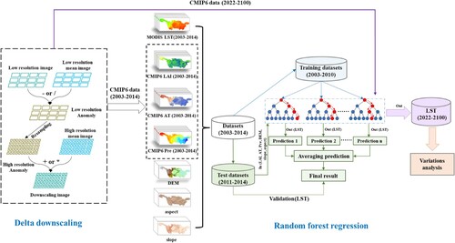
The Delta downscaling method was used to generate 1-km high-resolution Pre and AT datasets and 5-km LAI datasets. As part of the Bias Correction and Spatial Disaggregation (BCSD) method, Delta downscaling had been widely used in various studies because of its simplicity and high accuracy (Peng et al. 2017; Shui et al. 2019). The downscaling process was illustrated in Figure 2.

Figure 2. Flowchart of the methods used in the study.

Pre: (1) $\begin{array}{c}(\mathit{a}){\displaystyle \frac{{\mathit{X}}_{{\mathit{m}}_{\mathit{n}}}}{\overline{{\mathit{X}}_{{\mathit{a}}_{\mathit{n}}}}}={\mathit{E}}_{{\mathit{m}}_{\mathit{n}}}(\mathit{b}){\mathit{E}}_{{\mathit{m}}_{\mathit{n}}}\to {{\mathit{E}}^{\mathrm{\prime }}}_{{\mathit{m}}_{\mathit{n}}}(\mathit{c}){{\mathit{E}}^{\mathrm{\prime }}}_{{\mathit{m}}_{\mathit{n}}}\ast \overline{{\mathit{Z}}_{{\mathit{a}}_{\mathit{n}}}}={\mathit{Y}}_{{\mathit{m}}_{\mathit{n}}}}\end{array}$(1) AT or LAI: (2) $\begin{array}{c}(\mathit{a}){\mathit{X}}_{{\mathit{m}}_{\mathit{n}}}-\overline{{\mathit{X}}_{{\mathit{a}}_{\mathit{n}}}}={\mathit{E}}_{{\mathit{m}}_{\mathit{n}}}(\mathit{b}){\mathit{E}}_{{\mathit{m}}_{\mathit{n}}}\to {{\mathit{E}}^{\mathrm{\prime }}}_{{\mathit{m}}_{\mathit{N}}}(\mathit{c}){{\mathit{E}}^{\mathrm{\prime }}}_{{\mathit{m}}_{\mathit{n}}}+\overline{{\mathit{Z}}_{{\mathit{a}}_{\mathit{n}}}}={\mathit{Y}}_{{\mathit{m}}_{\mathit{n}}}\end{array}$(2) where $\mathit{m}$ was the annual time series value (2003–2014 and 2022–2100), $\mathit{n}$ was the monthly time series value (1–12), and $\mathit{a}$ was the annual time series value of the selected reference data (1970–2000 in Pre and AT, 2003–2014 in LAI). In this study, since there was no such long time series data for LAI, the reference period and historical period of LAI were selected as 2003–2014. ${\mathit{X}}_{{\mathit{m}}_{\mathit{n}}}$was a long time series with low-resolution data, $\overline{{\mathit{X}}_{{\mathit{a}}_{\mathit{n}}}}$ was the average of the low-resolution data in period $\mathit{a}$. ${\mathit{E}}_{{\mathit{m}}_{\mathit{n}}}$ was the low-resolution residual, ${{\mathit{E}}^{\mathrm{\prime }}}_{{\mathit{m}}_{\mathit{n}}}$ was the high-resolution residual. Low-resolution residuals were resampled to high-resolution residuals using bilinear interpolation (Peng et al. 2017). $\overline{{\mathit{Z}}_{{\mathit{a}}_{\mathit{n}}}}$was the average value of the high-resolution data in the corresponding period and ${\mathit{Y}}_{{\mathit{m}}_{\mathit{n}}}$ was the downscaled data.

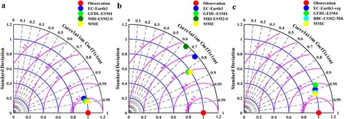
In order to reduce the error between different models, multi-model ensemble (MME) mean was performed for each climate variable. In addition, Taylor diagram was used to evaluate the simulation capability of the models (Feng 2022). The diagram included the correlation coefficient between model data and observed values, the ratio of standard deviations, and the ratio of root mean square error to standard deviation (RMSD). Generally speaking, a higher correlation coefficient and a smaller RMSD indicated the stronger the simulation ability of the model.

2.3.2. Random forest

Random forest (RF), a machine learning method widely used for classification and regression, was used in this study to establish nonlinear relationships between LST and predictor variables. The samples of each tree were randomly generated from the training samples, and the final prediction result was the average of the multiple regression trees. Compared with other regression models, the RF model has higher accuracy, strong generalization ability, and insensitivity to multicollinearity (Peng et al. 2021; Xiao et al. 2021). In this study, AT, Pre, LAI, DEM, slope and aspect were selected as the predictor variables. To unify the resolution of the data and reduce the amount of computation, we resampled all the datasets to 5-km. We selected data from 2003 to 2010 as the training datasets of the model and data from 2011 to 2014 as the testing datasets of the model. The predictor variables from 2022 to 2100 were then input into the trained model to calculate the corresponding LST (Figure 2). In the process of model training, max-depth and n-estimators, two important parameters were adjusted to prevent overfitting and thus obtain the best model. In this study, the n-estimators and max depth were 150 and 5, respectively, which were selected based on several tests.

2.3.3. Accuracy evaluation

To ensure the accuracy of the Delta downscaling and RF regression models, the root mean square error (RMSE), absolute mean error (MAE) and coefficient of determination (R²) were calculated to measure the accuracy. The RMSE and MAE indicated the deviation between the downscaled or predicted values and the actual values, and R² was often used to reflect the fit of the model (Wen et al. 2022). (3) $\begin{array}{c}RMSE=\sqrt{{\displaystyle \frac{{\sum }_{\mathit{i}=1}^{\mathit{n}}{({\mathit{A}}_{\mathit{i}}-{\mathit{P}}_{\mathit{i}})}^2}{\mathit{n}}}}\end{array}$(3) (4) $\begin{array}{c}MAE={\displaystyle \frac{{\sum }_{\mathit{i}=1}^{\mathit{n}}|{\mathit{P}}_{\mathit{i}}-{\mathit{A}}_{\mathit{i}}|}{\mathit{n}}}\end{array}$(4) (5) $\begin{array}{c}{\mathit{R}}^2={\displaystyle \frac{{\sum }_{\mathit{i}=1}^{\mathit{n}}{({\mathit{A}}_{\mathit{i}}-{\mathit{P}}_{\mathit{i}})}^2}{{\sum }_{\mathit{i}=1}^{\mathit{n}}{({\mathit{A}}_{\mathit{i}}-{\overline{\mathit{A}}}_{\mathit{i}})}^2}}\end{array}$(5) ${\mathit{A}}_{\mathit{i}}$ was the actual data, ${\mathit{P}}_{\mathit{i}}$ was the downscaled or predicted value, and $\mathit{n}$ was the number of effective pixels.

2.3.4. Temporal, spatial and trend analysis for LST

Absolute variability (AV) was used to measure the deviation of the data over a certain period relative to the multiyear average. The AV values of LST were related to short-term fluctuations in atmospheric circulation over time and space (Wei et al. 2021). (6) $\begin{array}{c}AV={\displaystyle \frac{{\sum }_{\mathit{i}=1}^{\mathit{n}}|{\mathit{x}}_{\mathit{i}}-{\mathit{m}}_{\mathit{X}}|}{\mathit{n}}}\end{array}$(6) ${\mathit{x}}_{\mathit{i}}$ was the LST value in year $\mathit{i}$, ${\mathit{m}}_{\mathit{X}}$ was the average from 2022 to 2100, and $\mathit{n}$ was number 79. We used the coefficient of variation (CV) to measure the spatial fluctuation of the AV in the YRB.

Additionally, this study also used the Sen’s trend estimator and Mann-Kendall (M-K) test, two nonparametric methods, to examine the trend of interannual and seasonal LST changes on the grid scales from 2022 to 2100 and to indicate whether the long-term trend was significant by using the statistic $|{\mathit{Z}}_{\mathit{S}}|$. $|{\mathit{Z}}_{\mathit{S}}|$>1.96 indicated that the time series trend was significant at 95% confidence level. Compared to the parameter trend test method, which required data to be independent and conformed to a normal distribution, the non-parametric trend test only required data to be independent. In this study, winter, spring, summer and autumn were from December (previous year) to February, March to May, June to August, and September to November, respectively. The RF model was constructed, and all statistical analyses were conducted using MATLAB R2017b.

3 . Results

3.1. Evaluation of downscaled AT, pre and LAI

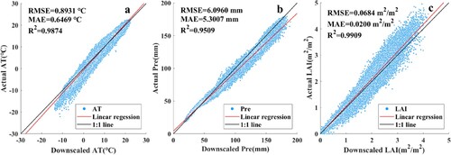
The spatial patterns of AT, Pre and LAI before and after downscaling were highly consistent (Figure 3a–f). The highest R² occurred in the downscaled LAI (0.9909), followed by the downscaled AT (0.9874), and downscaled Pre (0.9509) (Figure 4a–c). In the low temperature zone, mainly distributed in the western YRB, the downscaled AT was overestimated relative to the actual AT, but the overall error was smaller, with an RMSE of 0.8931 °C and MAE of 0.6469 °C. The RMSE and MAE (6.0960 mm and 5.3007 mm, respectively) of downscaled Pre and actual Pre demonstrated that the downscaling data were still reliable for analysis. The downscaled LAI and actual LAI were uniformly distributed around the 1:1 line, and there was a slight underestimation in the high value area. The RMSE and MAE of LAI were 0.0684 m²/m² and 0.0200 m²/m², respectively.

Figure 3. Spatial comparison of AT (a and d), Pre (b and e) and LAI (c and f) before and after downscaling. AT, Pre and LAI take August 2009 of GFDL-ESM4, March 2008 of GFDL-ESM4 and November 2014 of EC-Earth3-veg as examples, respectively.

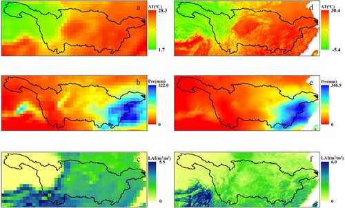
Figure 4. Relationship between downscaled values and actual values in monthly mean AT (a), Pre (b) and LAI (c).

The simulation capability of MME was superior to a single model in the three climate variables (Figure 5a–c). In terms of the correlation coefficient between MME and the actual value, AT was 0.99, LAI was 0.96, while Pre was 0.83. The RMSD was close to 0.2 for AT and LAI, and 0.6 for Pre. In a word, AT had the best simulation effect, followed by LAI and Pre.

Figure 5. Taylor diagrams for CMIP6 model and observed data. From left to right were AT (a), Pre (b) and LAI (c), respectively.

3.2. Evaluation of RF model accuracy

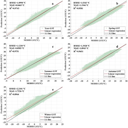
The scatter plots of the predicted LST and MODIS LST illustrated that the model exhibited good performance for interannual and seasonal LST predictions. The RMSEs varied from 1.0998 °C to 2.2101 °C, indicating that the predicted LST can effectively reflect the results of MODIS LST (Figure 6a–e). The smallest MAE arose in the prediction of interannual LST (0.8465 °C), followed by MAE of summer LST (0.8583 °C), and the MAE of other seasons were all above 1 °C. The R² values ranged from 0.8964 to 0.9743. The highest and lowest R² values occurred in summer and winter, respectively, and the R² values of all other seasons exceeded 0.9581. The summer LST of prediction and summer LST of MODIS were evenly distributed around the 1:1 line, coinciding with the linear regression line. The predicted LST in spring was underestimated in the high-temperature regions and underestimated in the low temperature regions. The predicted values of autumn LST were also overestimated in the low temperature regions.

Figure 6. The relationship between the predicted LST and MODIS LST in year (a), spring (b), summer (c), autumn (d) and winter (e).

3.3. Temporal changes of future LST

Interannual LST and seasonal LST fluctuated under the three scenarios, and the fluctuation of the spring LST was more drastic (Figure 7a–e). interannual LST increased by 0.546 °C, 1.170 °C and 2.129 °C under different scenarios, respectively (Table 3). Under the SSP1-2.6 scenario, the warming range of seasonal LST was 0.148–1.513 °C, and the maximum value occurred in winter. For SSP2-4.5 scenario, LST increased by more than 1 °C in autumn and winter, 0.741 °C and 0.772 °C in spring and summer, respectively. The seasonal LST under the SSP5-5.8 scenario had the largest warming amplitude relative to the other two scenarios. Spring, summer, autumn and winter LST increased by 1.693 °C, 1.295 °C, 1.654 °C and 3.674 °C, respectively (Table 3).

Figure 7. Temporal changes of interannual (a), spring (b), summer (c), autumn (d) and winter (d) LST under SSP1-2.6, SSP2-4.5, and SSP5-8.5 scenarios from 2022 to 2100. The shading is at the 95% confidence level.

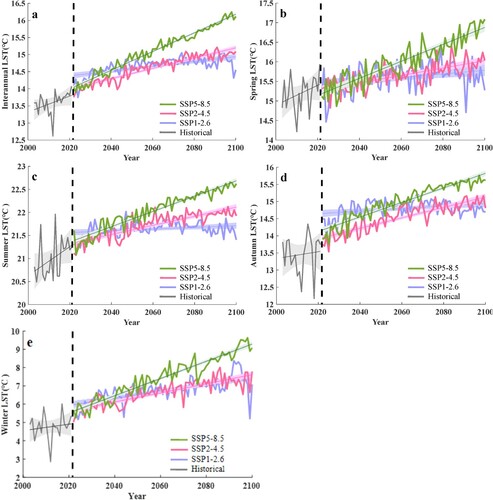
Table 3. The amplitude of changes in interannual and seasonal LST in the future period (°C).

	2022–2100			2025–2050			2050–2075			2075–2100
	SSP 1–2.6	SSP 2–4.5	SSP 5–8.5	SSP 1–2.6	SSP 2–4.5	SSP 5–8.5	SSP 1–2.6	SSP 2–4.5	SSP 5–8.5	SSP 1–2.6	SSP 2–4.5	SSP 5–8.5
Year	0.546	1.170	2.129	0.513	0.395	0.873	0.188	0.253	0.670	−0.078	0.073	0.780
Spring	0.359	0.741	1.693	0.753	0.220	0.563	0.083	−0.050	0.473	−0.380	0.105	0.840
Summer	0.148	0.772	1.295	0.308	0.270	0.640	0.060	0.133	0.438	−0.153	0.080	0.340
Autumn	0.289	1.186	1.654	0.755	0.500	0.888	0.230	0.238	0.550	−0.230	0.183	0.245
Winter	1.513	1.942	3.674	1.095	0.540	1.348	0.298	0.553	1.383	0.388	0.085	1.678

The amplitude changes in the recent period (2025–2050), middle period (2050–2075) and end period (2075–2100) were also different. Interannual and seasonal LST in the recent period showed an increasing trend in three scenarios, among which winter LST increased by more than 1 °C under SSP1-2.6 and SSP5-8.5 scenarios (Figure 7a–e) (Table 3). During the middle period, spring LST decreased by 0.050 °C under the SSP2-4.5 scenario and increased under the other scenarios. The remaining seasonal and interannual LST increased under all three scenarios. In the end period, LST exhibited an increasing trend under SSP2-4.5 and SSP5-8.5 scenarios, and the largest increase was in winter under SSP5-8.5 scenario, with an amplitude of 1.678 °C. LST under SSP1-2.6 scenario decreased by 0.078 °C in interannual LST, 0.380 °C in spring, 0.153 °C in summer, and 0.230 °C in autumn, respectively. While winter LST increased by 0.388 °C.

3.4. Spatial changes of future LST

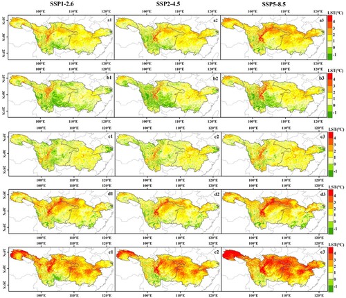
In both scenarios, interannual LST during 2022–2100 increased over a large area compared to the base period (2003–2021). The largest increment was located in the western border of the Chengdu Plain, while the LST of the southwest region of the UYRB decreased compared to the base period (Figure 8a1–a3). Spring LST increased significantly, mainly in the middle region of the UYRB, with an increment of more than 3 °C. The cooling area was larger than the interannual LST (Figure 8b1–b3). The increment in summer LST mainly concentrated between 1 and 2 °C under the SSP5-8.5 scenario. The spatial pattern in the other two scenarios was slightly different from that under the SSP5-8.5 scenario, which was mainly reflected in the obvious shrinkage of the warming area (Figure 8c1–c3). The spatial variation patterns of autumn LST under the three scenarios were essentially the same, with the larger increment region concentrated in the northern YRB and the cooling region concentrated in the northern Yunnan and Jiangxi (Figure 8d1–d3). There were clear spatial differences in winter LST variation compared to interannual and other seasons. The area with an increment greater than 3 °C was widely increased and scattered in all sub-basins of the YRB. The increment in SYRB was significantly higher than that in LYRB (Figure 8e1–e3).

Figure 8. Changes of LST in the future period (2022–2100) relative to the base period (2003–2021) in year (a1–a3), spring (b1–b3), summer (c1–c3), autumn (d1–d3) and winter (e1–e3) under SSP1-2.6 (a1–e1), SSP2-4.5 (a2–e2), and SSP5-8.5 (a3–e3) scenarios.

3.5. AV change

The interannual AV showed an increasing trend with increasing radiative forcing. Under SSP1-2.6 scenarios, the interannual AV values of the most regions were below 0.5 °C, and the mean value was 0.31 °C (Figure 9a). AV values of higher than 0.6 °C mainly occurred in the northern YRB under the SSP2-4.5 scenario (Figure 9b). Compared with the two scenarios described above, the AV value of SSP5-8.5 exhibited the largest spatial fluctuation (CV = 59.0%) (Table 4). The highest value was found in the SYRB, the western UYRB, and the northern MYRB, with a value surpassing 0.9 °C. Low values were mainly located in the eastern UYRB and southern MYRB (Figure 9c).

Figure 9. AV variation of the interannual LST from 2022 to 2100 under SSP1-2.6 (a), SSP2-4.5 (b) and SSP5-8.5 (c) scenarios.

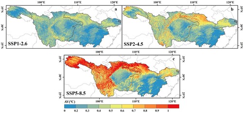
Table 4. Mean AV values (°C) and CV of year and four seasons under SSP1-2.6, SSP2-4.5 and SSP5-8.5 scenarios.

		SSP 1–2.6			SSP 2–4.5		SSP 5–8.5
	mean	std	CV	Mean	std	CV	mean	std	CV
year	0.31	0.13	41.9%	0.40	0.19	47.5%	0.36	0.61	59.0%
spring	0.47	0.16	34.0%	0.46	0.17	37.0%	0.64	0.31	48.4%
summer	0.28	0.13	46.4%	0.33	0.17	51.5%	0.42	0.24	57.1%
autumn	0.39	0.16	41.0%	0.50	0.21	42.0%	0.66	0.38	57.6%
winter	0.70	0.23	32.9%	0.74	0.25	33.8%	1.08	0.47	43.5%

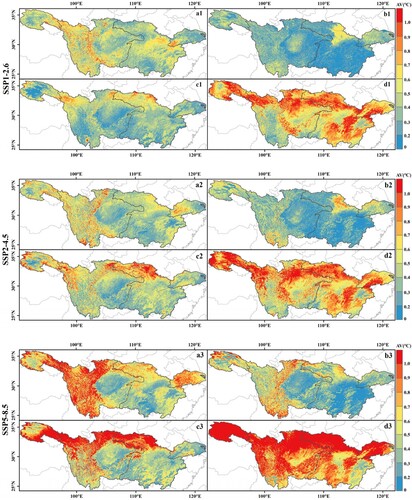
Similarly, AV increased sequentially from spring to winter, excluding summer, in the same scenario. In SSP1-2.6 scenario, winter AV had the smallest spatial variation (CV = 32.9%), and mean AV was 0.70 °C (Table 4). The low AV values were mainly observed in the southern UYRB (Figure 10d1). The AV values in summer were basically under 0.3 °C except for the northern UYRB (Figure 10b1). The mean AV values in spring and autumn reached 0.47 and 0.39 °C, respectively (Table 4). Meanwhile, spring AV showed moderate spatial variation, whereas autumn AV showed high spatial variation (CV = 34.0%, CV = 41.0%, respectively). In the SSP2-4.5, the spatial distribution of AV values in spring, summer and winter was similar to that in the SSP1-2.6. High AV values in autumn occurred in the northern YRB and the SYRB (Figure 10c2). For the SSP5-8.5 scenario, the four seasons showed high spatial fluctuation, with the value of CV greater than 43.5% (Table 4). High AV values were mainly distributed in the western YRB in spring, extended to the northern MYRB in autumn, and were distributed throughout the entire YRB in winter (Figure 10a3, c3–d3). The winter AV was greater than 0.9 °C in large areas, and the average value was 1.08 °C. The spatial distribution of low AV values remained consistent in spring, summer and autumn, and were mainly scattered in the eastern UYRB and the southern MYRB (Figure 10a3–c3).

Figure 10. AV variation of the spring (a1–a3), summer (b1–b3), autumn (c1–c3) and winter (d1–d3) LST from 2022 to 2100 under SSP1-2.6 (a1–d1), SSP2-4.5 (a2–d2), and SSP5-8.5 (a3–d3) scenarios.

3.6. Trend analysis

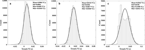
For the interannual LST under the three scenarios, over 87.5% area showed a significant warming trend during 2022–2100 (p < 0.05). Only northern Guizhou, southern Sichuan, northern Hunan and Jiangxi showed an inapparent cooling trend (p > 0.05) (Figure 11a–c). Under SSP1-2.6 scenario, the trend variation of LST varied from −0.0480 °C/y to 0.0628 °C/y, and the average variation rate was 0.0062 ± 0.0066 °C/y (p < 0.05) (Figure 12a). LST under SSP2-4.5 scenario warmed faster compared with SSP1-2.6 scenario, with an increase rate of 0.0143 ± 0.0079 °C/y (p < 0.05) (Figure 12b). The area with warming rate more than 0.02 °C/y (p < 0.05) was mainly located in the western UYRB and the northern YRB (Figure 11b). For SSP5-8.5 scenario, 93.7% of the area showed an upward trend. The warming rate of the SYRB, the western UYRB and Northern MYRB exceeded 0.04 °C/y (p < 0.05) (Figure 11c).

Figure 11. Trends of interannual LST under SSP1-2.6 (a), SSP2-4.5 (b) and SSP5-8.5 (c) scenarios. Pixels with significant changes (p < 0.05) were colored in yellow in the two insets.

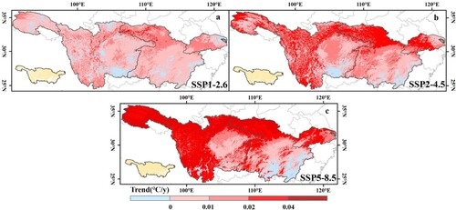
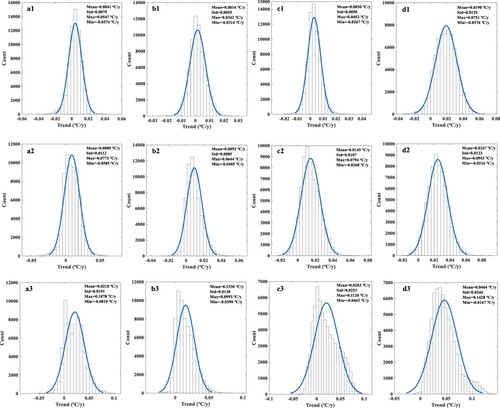
Figure 12. Histogram statistics under SSP1-2.6 (a), SSP2-4.5 (b) and SSP5-8.5 (c) scenarios.

At seasonal scale, the LST warming areas in spring, summer and autumn exceeded 60.4% under SSP1-2.6 scenario, and the areas with insignificant cooling were scattered throughout the whole YRB (p > 0.05) (Figure 13a1–a3). The trend of winter LST showed an apparent discrepancy with that in the other three seasons. The mean warming rate of winter LST reached 0.0190 ± 0.0129 °C/y (p < 0.05) (Figure 14d1), and the warming area reached 94.6%, which was much higher than the other three seasons (Figure 13d1). Meanwhile, an insignificant cooling trend was observed in the western UYRB. Under SSP2-4.5 scenario, The LST increased at an accelerated rate in four seasons, ranging from 0.0089 ± 0.0112 °C/y to 0.0247 ± 0.0123 °C/y (Figure 14a2–d2). 78.6% of the regions showed a remarkable upward trend (p < 0.05) in spring LST, mainly distributed in the regions except northern Guizhou and southern LYRB (Figure 13a2). The warming area of summer LST increased by 10.2% compared to spring LST, mainly located in northern Guizhou (Figure 13b2). The autumn LST was characterized by extensive warming, with a warming area of 93.4%, and there was no obvious cooling area (Figure 13c2). In 98.6% region, winter LST exhibited a significant warming trend (p < 0.05) and the rate was more than 0.01 °C/y (Figure 13d2). The LST under the SSP5-8.5 scenario presented characteristics of extensive and rapid increases. In spring, the warming rate of the SYRB, the western UYRB, the northern MYRB and the LYRB exceeded 0.03 °C/y (p < 0.05) (Figure 13a3). The spatial pattern of warming in autumn LST was similar to that in spring LST, except for LYRB. However, the LST in autumn had a significant cooling area of 24.5% (p < 0.05), mainly scattered in Chongqing and the southern MYRB (Figure 13c3). Although the average warming rate of summer LST was the lowest of the four seasons, with a warming rate of 0.0153 ± 0.0130 °C/y, it still exhibited a warming area of 92.0% (Figure 13b3 and Figure 14b3). The LST warmed 99.7% of the area during winter. Except for the southern MYRB, the increase rate of LST was greater than 0.03 °C/y (p < 0.05), and the highest value was 0.14 °C/y (p < 0.05) (Figure 13d3 and Figure 14d3).

Figure 13. Trends of spring (a1–a3), summer (b1–b3), autumn (c1–c3) and winter (d1–d3) LST under SSP1-2.6 (a1–d1), SSP2-4.5 (a2–d3) and SSP5-8.5 (a3–d3) scenarios. Pixels with significant changes (p < 0.05) were colored in yellow in the two insets.

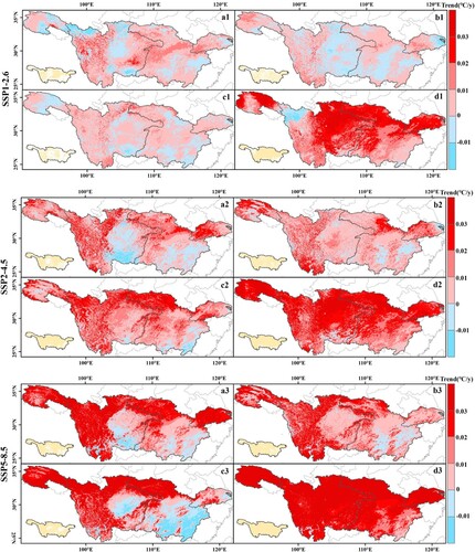
Figure 14. histogram statistics under SSP126 (a1–d1), SSP245 (a1–d2) and SSP585 (a3–d3) scenarios in spring (a1–a3), summer (b1–b3), autumn (c1–c3) and winter (d1–d3).

4. Discussion

Historical observations had shown that global temperature was in a stage of continuous warming, and the YRB had a positive response to global warming (Huang, Li, and Song 2022; Liu et al. 2022). Nevertheless, future changes in the YRB remain unclear. In this study, high-resolution AT, Pre and LAI data under three SSP scenarios of the CMIP6 model were generated based on the Delta spatial downscaling method. High-resolution LST data from 2022 to 2100 were calculated by combining LST during 2003–2021, elevation, slope and aspect. Therefore, the inability to analyze future LST changes was solved in the YRB.

The annual mean LST of the YRB continued to warm at an accelerated rate under the three SSP scenarios, particularly in the northern and western YRB (southeast of the Tibetan Plateau) under the SSP2-4.5 and SSP5-8.5 scenarios (Figure 11c). Rapid warming of western YRB would affect the future ecological environment and water resource availability (You et al. 2021). The SYRB was distributed in many snow-capped mountains and frozen soil, such as the Geladandong snow-capped mountains in the western YRB. Future warming would lead to accelerated melting of snow and glaciers, potentially causing flooding or waterlogging in the MYRB and LYRB, and disruption of hydrological systems (You et al. 2019; You et al. 2020). Yue (2022) also deemed that the YRB would face a higher flood disaster threat index and wider flood area in the future. Therefore, flood protection measures needed to be developed to ensure that they could be implemented when disasters occurred. With the increase of LST in the future, the frequency and severity of drought events caused by increased evapotranspiration would increase (Zuo et al. 2019). For example, extreme heat events in Europe in 2003 and Russia in 2010 exacerbated drought pressures (He et al. 2023). Similarly, the YRB had the characteristics of short-term fluctuation of drought and coexistence of drought and flood, so the study of drought scenario deserved more attention. An increase in LST may also inhibit future vegetation growth, leading to a weakened carbon sequestration capacity. A recent study showed that, although CO₂ increase was the main driver of vegetation greening, the negative impact of global warming on vegetation offset part of the increase, which meat that future vegetation greening may be limited (Zhao et al. 2020). The National Climate Change Assessment report released by the Chinese government in 2006 predicted that China’s temperature would continue to rise from 2020 to 2100, particularly in winter, which was consistent with our research results (Ding et al. 2006). Currently, the increase in anthropogenic greenhouse gas emissions was considered to be the main cause of global temperature rise (Yang et al. 2021). Our results also showed that winter LST warming was faster under the SSP5-8.5 scenario (Figure 13d1–d3). Examining the response of temperature warming to external forcing revealed that human influence could be detected in seasonal changes, with the strongest in winter. According to previous studies, China was the world’s largest carbon emitter, with an increase of 0.64 °C per unit ppm (Qian and Zhang 2019; Ying et al. 2021). Coupled with the complex topography of the YRB, with high altitudes and large topographic differences, greenhouse gas emissions were more destructive to this region than to other regions (Zhou et al. 2022). Topographic effects may also be one of the reasons for the significant increase of future LST in the western Sichuan basin relative to the base period (Tian et al. 2022). In addition, Chengdu, Mianyang and Deyang had experienced rapid urbanization in recent years. It was found that the warming effect of urbanization increased turbulence, which in turn increased boundary temperature (Yao 2020). If the urbanization level continued to increase in the future, then the Sichuan basin LST may increase further.

The AV values of LST could explain the fluctuations in regional atmospheric circulation (Wei et al. 2021). High AV values were mainly distributed in the western and northern YRB, mainly due to the long-term control of the Western Pacific Subtropical High pressure (WPSH) and Indian summer monsoon over the YRB (Figures 9 and 10) (Guan et al. 2010; Huang et al. 2021). The prevailing downdraft was conducive to surface warming, and under the action of a large area of high pressure, high temperature was frequent and intense, which was also the reason for the continuous high temperature and drought in the YRB. Simultaneously, the alternate occurrence of El Niño and La Niña stimulated atmospheric fluctuations, thus affecting the position of the WPSH (Zhang, Xu, and Shi 2015). In addition, we found that the AV values in the SSP5-8.5 scenario were larger than those in the other two scenarios (Figure 10). A previous study by Yang et al. (2022) showed that under the SSP5-8.5 scenario, the event frequency of strong WPSH would increase in the future. This was mainly due to the enhanced response of Pre and atmospheric convection to sea surface temperature changes caused by global warming.

In the original CMIP6 models, there were many reasons for the errors, such as the complexity of climatic causes and differences in topography and underlying surface. And larger errors tended to be concentrated in areas with less human activity, such as the Tibetan Plateau (Fan et al. 2020). Previous studies had found that high-resolution reference climate datasets with topographic effects could generate downscaling data with higher spatial resolution and correction errors (Peng et al. 2019). The WorldClim climate data not only achieved satisfactory results in previous studies, but also relatively reliable results in this study. In addition, the resolution of downscaling data depended on the resolution of reference data, and the development of higher resolution climate data would significantly improve the spatial resolution of downscaling. It was worth noting that even if the Delta spatial downscaling method could introduce the effect of terrain, it still could not completely eliminate the deviation. It was found that the AT was overestimated in the low temperature region, and the error source was mainly in the spring (Table 5). The evaluation results of the CMIP6 model showed that AT has some errors in areas with complex terrain (Zhang et al. 2022). The downscaled Pre in the YRB was overestimated overall, which was consistent with the results of Feng (2022). These phenomena meant that the CMIP6 model still had a defect in the process of reproducing the atmosphere of complex terrain, which was consistent with the findings reported in CMIP5 and CMIP6 (You et al. 2021; Feng 2022; Zhang et al. 2022). The downscaling of Pre had been difficult, and many studies had shown that the downscaling effect of Pre in different regions was worse than that of AT, and so were our results (Shui et al. 2019; Feng et al. 2022). Although previous studies did not conduct spatial downscaling for LAI, from the perspective of the CMIP6 LAI assessment, MME could better simulate the spatial and temporal distribution of LAI in China (Sun, Xue, and Zhou 2023). Meanwhile, from the downscaling results of this study, LAI showed a lower error and higher R² in both years and seasons.

Table 5. Downscaling errors of AT, Pre and LAI in year, spring, summer, autumn and winter.

	Pre (mm)			AT (°C)			LAI
	RMSE	MAE	R^2	RMSE	MAE	R^2	RMSE	MAE	R^2
spring	9.847	6.915	0.967	1.269	0.960	0.976	0.114	0.088	0.978
summer	14.965	12.239	0.790	0.772	0.590	0.991	0.091	0.070	0.993
autumn	7.803	6.586	0.857	0.973	0.697	0.986	0.074	0.056	0.998
winter	3.909	2.410	0.972	0.910	0.605	0.986	0.097	0.064	0.945

As for the RF model, we found that there was still an overestimation or underestimation problem with an overall higher performance (Figure 6). By comparing the performance of the three trees when n-estimators were 50, 150 and 250, it was found that the accuracy of 150 was slightly improved compared with that of 50. Nevertheless, performance decreased when the n-estimators were 250 (Table 6). This indicated that our model achieved the best performance in this study. Therefore, the overestimation or underestimation problem in this region was not due to the parameter setting. Wang (2022) also found overestimation when using RF model to predict NPP in the Guangdong-Hong Kong-Macao Greater Bay Area. He believed that even if the resolution of CMIP6 data were improved by downscaling, it would still cause errors, which would lead to algorithm errors in model construction. Our downscaling results for the three climate variables showed overestimation and underestimation in different regions, especially in spring, which indirectly explained the uncertainty in the RF model. In addition, changes in LST were influenced by many factors (Yang et al. 2021). For example, the net radiation balance formula showed that LST was related to downward shortwave radiation and upward longwave radiation (Liu et al. 2022). Moreover, changes in cloud cover, aerosols and land use could also drive LST changes. Thus, increasing the predictable variables and sample size may also be a way to improve the accuracy of the model.

Table 6. Comparison of regression tree performance.

	n-estimators = 50			n-estimators = 150			n-estimators = 250
	MAE	RSME	R^2	MAE	RSME	R^2	MAE	RSME	R^2
year	0.8483	1.1025	0.9742	0.8465	1.0998	0.9743	0.8466	1.0999	0.9743
spring	1.2024	1.5448	0.9552	1.1944	1.5343	0.9581	1.1967	1.5375	0.9556
summer	0.8605	1.1240	0.9750	0.8583	1.1210	0.9751	0.8594	1.1223	0.9750
autumn	1.0987	1.4166	0.9601	1.0943	1.3928	0.9651	1.0932	1.4099	0.9604
winter	1.7243	2.2127	0.8961	1.7226	2.2101	0.8964	1.7242	2.2115	0.8962

5. Conclusion

In this study, the Delta spatial downscaling method was used to improve the resolution of the Pre, AT and LAI of CMIP6. The results showed that the data after downscaling had high accuracy and MME could effectively reflect the actual climate variables. As a simple spatial scaling method, delta was suitable for small and medium research areas to achieve rapid and effective spatial downscaling. On this basis, we built a RF model to calculate the LST data from 2022 to 2100. The performance evaluation showed that the RF model could effectively predict the LST in the YRB. However, the problem of overestimation and underestimation still existed, therefore, the performance of the model should be improved to enhance the prediction accuracy in the future. The results of future LST analysis showed that the warming rate of SSP5-8.5 was the fastest, followed by SSP2-4.5, and SSP1-2.6 was the slowest. During 2075–2100, the LST under the SSP1.2-6 scenario had a downward trend, except in winter. The future LST in western Sichuan basin would increase obviously compared with the base period. Secondly, at both annual and seasonal scales, the LST under the SSP5-8.5 scenario had the largest fluctuation, especially in the western and northern YRB. Finally, 87.5% of the area showed a warming trend in the interannual LST under three scenarios. From a seasonal perspective, the area and rate of LST warming in winter under the three scenarios were significantly higher than those during the other three seasons.

Disclosure statement

No potential conflict of interest was reported by the author(s).

Additional information

Funding

This work was supported by the National Natural Science Foundation of China (U2244216), the National key R&D plan (2022YFF0802101), the Fundamental Research Funds for the Central Universities (SWU-KT22009), and the Key Project of Innovation LREIS (KPI001).

References

- Bartkowiak, P., M. Castelli, and C. Notarnicola. 2019. “Downscaling Land Surface Temperature from MODIS Dataset with Random Forest Approach Over Alpine Vegetated Areas.” Remote Sensing 11: 1319. https://doi.org/10.3390/rs11111319.
- Ding, Y., and S. Peng. 2021. “Spatiotemporal Change and Attribution of Potential Evapotranspiration Over China from 1901 to 2100.” Theoretical and Applied Climatology 145 (1-2): 79–94. https://doi.org/10.1007/s00704-021-03625-w.
- Ding, Y., G. Ren, G. Shi, P. Gong, Z. Hua, P. Zhai, D. Zhang, Z. Ci, S. Wang, H. Wang, et al. 2006. “National Assessment Report of Climate Change (i): Climate Change in China and its Future Trend.” Advances in Climate Change Research 2: 3–8.
- Du, Z., J. Zhao, X. Liu, Z. Wu, and H. Zhang. 2019. “Recent Asymmetric Warming Trends of Daytime Versus Nighttime and Their Linkages with Vegetation Greenness in Temperate China.” Environmental Science and Pollution Research 26 (35): 35717–35727. https://doi.org/10.1007/s11356-019-06440-z.
- Fan, X. X., Q. Y. Duan, C. W. Chen, Y. Wu, and C. Xing. 2020. “Global Surface Air Temperatures in CMIP6: Historical Performance and Future Changes.” Environmental Research Letters 15 (10): 104056. https://doi.org/10.1088/1748-9326/abb051.
- Feng, W. 2022. “Spatial-Temporal Variation and Prediction of NPP in the Yangtze River Basin Based on CASA Model and CMIP6 Model.” PhD diss., Southwest university.
- Feng, Y., Z. He, S. Jiao, and W. Liu. 2022. “Scenario Prediction of Extreme Precipitation in Guizhou Province Based on CMIP6 Climate Model.” Research of Soil and Water Conservation, 1–9. https://doi.org/10.13869/j.cnki.rswc.20220621.004.
- Guan, Z., J. Cai, W. Tang, and Y. Bai. 2010. “Variations of West Pacific Subtropical High Associated with Principal Patterns of Summertime Temperature Anomalies in the Middle and Lower Reaches of the Yangtze River.” Journal of the Meteorological Sciences 5: 666–675.
- He, B., W. Wang, A. Sharifi, and X. Liu. 2023. “Progress, Knowledge Gap and Future Directions of Urban Heat Mitigation and Adaptation Research Through a Bibliometric Review of History and Evolution.” Energy and Buildings 287: 112976–117788. https://doi.org/10.1016/j.enbuild.2023.112976.
- Huang, J., Q. Li, and Z. Song. 2022. “Historical Global Land Surface Air Apparent Temperature and Its Future Changes Based on CMIP6 Projections.” Science of The Total Environment 816: 151656. https://doi.org/10.1016/j.scitotenv.2021.151656.
- Huang, X., S. Yang, A. Haywood, D. Jiang, Y. Wang, M. Sun, Z. Tang, and Z. Ding. 2021. “Warming-Induced Northwestward Migration of the Asian Summer Monsoon in the Geological Past: Evidence from Climate Simulations and Geological Reconstructions.” Journal of Geophysical Research: Atmospheres 126: e2021JD03590. https://doi.org/10.1029/2021JD035190.
- Jia, H., D. Yang, W. Deng, Q. Wei, and W. Jiang. 2021. “Predicting Land Surface Temperature with Geographically Weighed Regression and Deep Learning.” WIRES Data Mining and Knowledge Discovery 11: e1396. https://doi.org/10.1002/widm.1396.
- Li, Z., F. Zheng, W. Liu, and D. Jiang. 2012. “Spatially Downscaling GCMs Outputs to Project Changes in Extreme Precipitation and Temperature Events on the Loess Plateau of China During the 21st Century.” Global and Planetary Change 82-83: 65–73. https://doi.org/10.1016/j.gloplacha.2011.11.008.
- Liu, J., S. Liu, X. Tang, Z. Ding, M. Ma, and P. Yu. 2022. “The Response of Land Surface Temperature Changes to the Vegetation Dynamics in the Yangtze River Basin.” Remote Sensing 14: 5093. https://doi.org/10.3390/rs14205093.
- Mao, K., Y. Yan, M. Cao, Z. Yuan, and Z. Qin. 2020. “Reconstruction of Surface Temperature Data and Analysis of Spatial and Temporal Changes in North America.” Remote Sensing for Natural Resources, 1–13. https://doi.org/10.6046/zrzyyg.2021254.
- Masson-Delmotte, V., P. Zhai, A. Pirani, S. Connors, C. Péan, S. Berger, et al. 2021. “Climate Change 2021: The Physical Science Basis.” Contribution of Working Group I to the Sixth Assessment Report of the Intergovernmental Panel on Climate Change 2.
- Mohammad, P., and A. Goswami. 2021. “A Spatio-Temporal Assessment and Prediction of Surface Urban Heat Island Intensity Using Multiple Linear Regression Techniques Over Ahmedabad City, Gujarat.” Journal of the Indian Society of Remote Sensing 49 (5): 1091–1108. https://doi.org/10.1007/s12524-020-01299-x.
- Peng, S., Y. Ding, W. Liu, and Z. Li. 2019. “1 km Monthly Temperature and Precipitation Dataset for China from 1901 to 2017.” Earth System Science Data 11: 1931–1946. https://doi.org/10.5194/essd-11-1931-2019.
- Peng, S., Y. Ding, Z. Wen, Y. Chen, Y. Cao, and J. Ren. 2017. “Spatiotemporal Change and Trend Analysis of Potential Evapotranspiration Over the Loess Plateau of China During 2011–2100.” Agricultural and Forest Meteorology 233: 183–194. https://doi.org/10.1016/j.agrformet.2016.11.129.
- Peng, W., X. Yuan, W. Gao, R. Wang, and W. Chen. 2021. “Assessment of Urban Cooling Effect Based on Downscaled Land Surface Temperature: A Case Study for Fukuoka, Japan.” Urban Climate 36: 100790. https://doi.org/10.1016/j.uclim.2021.100790.
- Qian, C., and X. Zhang. 2019. “Changes in Temperature Seasonality in China: Human Influences and Internal Variability.” Journal of Climate 32 (19): 6237–6249. https://doi.org/10.1175/JCLI-D-19-0081.1.
- Schwingshackl, C., M. Hirschi, and S. Seneviratne. 2018. “Global Contributions of Incoming Radiation and Land Surface Conditions to Maximum Near-Surface Air Temperature Variability and Trend.” Geophysical Research Letters 45 (10): 5034–5044. https://doi.org/10.1029/2018GL077794.
- Shui, J., J. Ren, S. Peng, and X. Zhan. 2019. “A Dataset of 1 km-Spatial-Resolution Monthly Mean Temperature and Monthly Precipitation in the Loess Plateau from 1901 to 2014.” Science Data Bank 4: 133–142. https://doi.org/10.5194/essd-11-1931-2019.
- Song, Z., H. Yang, X. Huang, W. Yu, J. Huang, and M. Ma. 2021. “The Spatiotemporal Pattern and Influencing Factors of Land Surface Temperature Change in China from 2003 to 2019.” International Journal of Applied Earth Observation and Geoinformation 104: 102537. https://doi.org/10.1016/j.jag.2021.102537.
- Sun, X., W. Xue, and B. Zhou. 2023. “CMIP6 Evaluation and Projection of Terrestrial Ecosystem Over Asia.” Climate Change Research 19: 49–65. https://doi.org/10.12006/j.issn.1673-1719.2022.045.
- Tang, C., X. Tao, C. Dai, and H. Wei. 2022. “Spatiotemporal Modal Analysis and Prediction of Surface Temperature in East Asia and the Western Pacific.” Journal of Tropical Oceanography, 1–10. https://doi.org/10.11978/2022009.
- Tian, H., L. Liu, Z. Y. Zhang, H. J. Chen, X. Y. Zhang, T. X. Wang, and Z. W. Kang. 2022. “Spatiotemporal Diversity and Attribution Analysis of Land Surface Temperature in China from 2001 to 2020.” Acta Geographica Sinica 77 (07): 1713–1729. https://doi.org/10.11821/dlxb202207010.
- Timm, O., T. Giambelluca, and H. Diaz. 2015. “Statistical Downscaling of Rainfall Changes in Hawai‘i Based on the CMIP5 Global Model Projections.” Journal of Geophysical Research: Atmospheres 120 (1): 92–112. https://doi.org/10.1002/2014JD022059.
- Tokarska, K., M. Stolpe, S. Sippel, E. Fischer, C. Smith, F. Lehner, and R. Knutti. 2020. “Past Warming Trend Constrains Future Warming in CMIP6 Models.” Science Advances 6 (12): eaaz9549. https://doi.org/10.1126/sciadv.aaz9549.
- Wang, Z. Y. 2022. “NPP Estimation of Terrestrial Ecosystems Under CMIP6 ScenarioMIP Based on Random Forest: A Case Study of the Guangdong-Hong Kong-Macao Greater Bay Area.” PhD diss.., Jiangxi University of Science and Technology.
- Wang, G., Y. He, B. Zhang, X. Wang, S. Cheng, Y. Xie, S. Wang, and S. Guan. 2023. “Historical Evaluation and Projection of Precipitation Phase Changes in the Cold Season Over the Tibetan Plateau Based on CMIP6 Multimodels.” Atmospheric Research 281: 106494. https://doi.org/10.1016/j.atmosres.2022.106494.
- Wei, B., Y. Bao, S. Yu, S. Yin, and Y. Zhang. 2021. “Analysis of Land Surface Temperature Variation Based on MODIS Data a Case Study of the Agricultural Pastural Ecotone of Northern China.” International Journal of Applied Earth Observation and Geoinformation 100: 102342. https://doi.org/10.1016/j.jag.2021.102342.
- Wen, A., T. Wu, X. Wu, X. Zhu, R. Li, J. Ni, G. Hu, Y. Qiao, D. Zou, J. Chen, et al. 2022. “Evaluation of MERRA-2 Land Surface Temperature Dataset and its Application in Permafrost Mapping Over China.” Atmospheric Research 279: 106373. https://doi.org/10.1016/j.atmosres.2022.106373.
- Xiao, Y., W. Zhao, M. Ma, and K. He. 2021. “Gap-free LST Generation for MODIS/Terra LST Product Using a Random Forest-Based Reconstruction Method.” Remote Sensing 13: 2828. https://doi.org/10.3390/rs13142828.
- Xu, B., J. Li, T. Park, Q. Liu, Y. Zeng, G. Yin, J. Zhao, W. Fan, L. Yang, and Y. Knyazikhin. 2018. “An Integrated Method for Validating Long-Term Leaf Area Index Products Using Global Networks of Site-Based Measurements.” Remote Sensing of Environment 209: 134–151. https://doi.org/10.1016/j.rse.2018.02.049.
- Yang, K., W. Cai, G. Huang, K. Hu, B. Ng, and G. Wang. 2022. “Increased Variability of the Western Pacific Subtropical High Under Greenhouse Warming.” Proceedings of the National Academy of Sciences 119 (23): e2120335119. https://doi.org/10.1073/pnas.2120335119.
- Yang, M., W. Zhao, Q. Zhan, and D. Xiong. 2021. “Spatiotemporal Patterns of Land Surface Temperature Change in the Tibetan Plateau Based on MODIS/Terra Daily Product from 2000 to 2018.” IEEE Journal of Selected Topics in Applied Earth Observations and Remote Sensing 14: 6501–6514. https://doi.org/10.1109/JSTARS.2021.3089851.
- Yao, Y. Q. 2020. “Land use in Sichuan Basin and Meteorological Effect of Urbanization in Chengdu Area.” PhD diss., Chengdu University of Information Technology.
- Ying, N., W. Wang, J. Fan, D. Zhou, Z. Han, Q. Chen, Q. Ye, and Z. G. Xue. 2021. “Climate Network Approach Reveals the Modes of CO2 Concentration to Surface air Temperature.” Chaos: An Interdisciplinary Journal of Nonlinear Science 31 (3): 031104. https://doi.org/10.1063/5.0040360.
- You, Q., Z. Cai, F. Wu, Z. Jiang, N. Pepin, and S. Shen. 2021. “Temperature Dataset of CMIP6 Models Over China: Evaluation, Trend and Uncertainty.” Climate Dynamics 57 (1-2): 17–35. https://doi.org/10.1007/s00382-021-05691-2.
- You, Q., F. Wu, H. Wang, Z. Jiang, N. Pepin, and S. Kang. 2020. “Projected Changes in Snow Water Equivalent Over the Tibetan Plateau Under Global Warming of 1.5° and 2°C.” Journal of Climate 33: 5141–5154. https://doi.org/10.1175/JCLI-D-19-0719.1.
- You, Q., Y. Zhang, X. Xie, and F. Wu. 2019. “Robust Elevation Dependency Warming Over the Tibetan Plateau Under Global Warming of 1.5 °C and 2 °C.” Climate Dynamics 53 (3-4): 2047–2060. https://doi.org/10.1007/s00382-019-04775-4.
- Yu, P. J., J. L. Liu, H. Y. Tang, X. Z. Sun, S. W. Liu, X. G. Tang, Z. Ding, M. G. Ma, and E. Ci. 2023. “Establishing a Soil Quality Index to Evaluate Soil Quality After Afforestation in a Karst Region of Southwest China.” CATENA 230: 107237. https://doi.org/10.1016/j.catena.2023.107237.
- Yue, Y. L. 2022. “The Changes of Future Runoff and Drought and Flood in the Yangtze River Basin Under Climate Change.” PhD diss., East China Normal University.
- Zafra, C., Y. Ángel, and E. Torres. 2017. “ARIMA Analysis of the Effect of Land Surface Coverage on PM 10 Concentrations in a High-Altitude Megacity.” Atmospheric Pollution Research 8 (4): 660–668. https://doi.org/10.1016/j.apr.2017.01.002.
- Zhang, J. Y., Y. R. Lun, Y. X. Liu, X. Li, and Z. X. Xu. 2022. “CMIP6 Evaluation and Projection of Climate Change in Tibetan Plateau.” Journal of Beijing Normal University (Natural Science) 58: 77–89. https://doi.org/10.12202/j.0476-0301.2021114.
- Zhang, Y. Y., H. M. Xu, and N. Shi. 2015. “Influence of Spring Arctic Oscillation on Surface Air Temperature Over Yangtze River Basin in Mid-Summer.” Chinese Journal of Atmospheric Sciences 39: 1049–1058. https://doi.org/10.3878/j.issn.1006-9895.1501.14238.
- Zhao, Q., Z. C. Zhu, H. Zeng, W. Q. Zhao, and R. B. Myneni. 2020. “Future Greening of the Earth May not be as Large as Previously Predicted.” Agricultural and Forest Meteorology 292-293: 108111–101923. https://doi.org/10.1016/j.agrformet.2020.108111.
- Zhou, M., Z. Yu, H. Gu, Q. Ju, Y. Gao, L. Wen, T. K. Huang, and W. Wang. 2022. “Evaluation and Projections of Surface air Temperature Over the Tibetan Plateau from CMIP6 and CMIP5: Warming Trend and Uncertainty.” Climate Dynamics, 3863–3883. https://doi.org/10.1007/s00382-022-06518-4.
- Zhu, H., Z. Jiang, and L. Li. 2021. “Projection of Climate Extremes in China, an Incremental Exercise from CMIP5 to CMIP6.” Science Bulletin 66 (24): 2528–2537. https://doi.org/10.1016/j.scib.2021.07.026.
- Zuo, D. P., S. Y. Cai, Z. X. Xu, D. Z. Peng, G. Y. Kan, W. C. Sun, B. Pang, and H. Yang. 2019. “Assessment of Meteorological and Agricultural Droughts Using in-Situ Observations and Remote Sensing Data.” Agricultural Water Management 222: 125–138. https://doi.org/10.1016/j.agwat.2019.05.046.