ROI-constrained visualization of flood scenes to improve perception efficiency

ABSTRACT

Efficient and intuitive representation of floods can improve people’s perception, which is useful for flood emergency management and decision making. However, the current methods of visualizing flood disaster scenes have the shortcomings of data redundancy and low-efficiency. The interference of the complex background can be avoided through region of interest (ROI) extraction, because the attention will be quickly attracted by a few salient visual objects. First, the characteristics of the flood disaster scene object are analysed, and the method for scene division and data organization is established. Second, the region of interest is extracted according to the time series data of the flood evolution process simulated using cellular automata, and the dynamic identification model of the objects of interest is established. Then, a dynamic scheduling queue model with service interruption is designed to optimize the rendering efficiency of flood scenes and improve the perception efficiency. Finally, a prototype visualization system was developed and the experimental results show that approximately 30% of the redundant data are reduced, and the scene rendering efficiency is increased by approximately 15%. The non-ROI visualization is weakened by using the rules of human visual cognition, which improves the perception efficiency of flood scenes.

KEYWORDS:

• Floods
• region of interest
• perception efficiency
• 3D scenes
• adaptive optimization

1. Introduction

As one of the most serious natural disasters, flood disasters always cause serious losses and have broad implications (Peden, Mayhew, and Baker 2022; Schröter et al. 2021; Tierolf, Moel, and Vliet 2021; Zhang et al. 2022). Floods pose a serious threat to urban development due to the concentration of economic activity, infrastructure and population (Romero and Leandro 2022; Totschnig and Fuchs 2013). According to statistics from the Global Disaster Data Platform, from 2011 to 2020, the average annual number of people affected by floods in the world was as high as 50 million, and 43,960 people were missing and died during this period. To tackle flood-related risk challenges, the conceptualization and visualization of flood risk systems provides insights which might help to provide guidance for flood emergency management, post-disaster assessment, and long-term flood adaptation planning (Li et al. 2022a; 2022b; Mai et al. 2020; Pugliese et al. 2022; Zhuo and Han 2020).

Flood visualization, which uses graphical language to visually represent floods, can convey useful information from abstract flood data and is beneficial to disaster prevention, mitigation and relief tasks such as post-disaster assessment, reconstruction, and disaster education (Lim, Brandt, and Seipel 2015; Minano et al. 2021; Seipel and Lim 2017; Zhang et al. 2020b). In particular, the development of Earth Observing Technology, 3DGIS, virtual geographic environment and other technologies has greatly enhanced the expression, interpretation and use of flood information, and improved people's cognitive level and awareness of disaster prevention and mitigation (Haynes, Hehl-Lange, and Lange 2018; Hernández et al. 2022; Hu et al. 2018; Li et al. 2021b; Spero et al. 2022; Wilkinson et al. 2015). Detailed 3D city model is very valuable and useful, which can be used for accurate spatial analysis and geographical calculation (Biljecki, Ledoux, and Stoter 2017; Bittner et al. 2018; Bshouty, Shafir, and Dalyot 2020; Nouvel et al. 2017). For example, Feng et al. (2022) extracted the facade openings of urban buildings (such as basement windows, doors, and underground garage entrances, etc.), which can help identify places that are more susceptible to water ingress during flooding. At the same time, efficient scene visualization is also essential, for it can effectively support the accurate transmission of geographic information (Zhang et al. 2020d). However, the high precision of scene data and the high efficiency of visualization are mutually restricted, and limited computer resources cannot cope with the efficient rendering of massive scene data. Inefficient and unclear expressions may lead to poor user experience and cannot support scientific decision-making.

The existing methods for flood scenes optimization are through visibility culling (Andújar, Vázquez, and Navazo 2000; Mao, Harrie, and Ban 2012; Yılmaz and Güdükbay 2007), model simplification (Li and Nan 2021; Liu et al. 2017), GPU unit programming (Fu, Yang, and Chen 2021a; Zhang, Wei, and Xu 2020a), dynamic scheduling based on external storage (Song and Li 2018), data caching and prescheduling (Zhang et al. 2017; Zhang et al. 2020c) and parallel computing (Huang, Chen, and Zhou 2020; She et al. 2017). On the other hand, some studies have shown that the multilevel representation of virtual scenes plays a crucial role in scene optimization. For example, Yao et al. (2017) proposed a method for building and scheduling the rendering of quadtrees for 3D models of the city based on rendering weights. Chen et al. (2018) used local curvature entropy to optimize 3D terrain. Li et al. (2021a) selected terrains with better geometric and shading details using summed-area tables (SATs).

Although certain improvements have been achieved using the above methods, the laws of human visual cognition are not considered. The theory of visual attention (TVA) shows that when the human visual system is faced with a complex scene, the attention will be quickly attracted by a few salient visual objects, and these objects will be preferentially processed (Carrasco 2011; Xie et al. 2022). Through ROI extraction, the interference of the complex background of the noninterest area can be avoided and the processing efficiency can be improved (Li and Dong 2013). Therefore, it has been widely employed in image object recognition, tracking and classification (Cheng and Buckles 2014; Saligrama, Konrad, and Jodoin 2010). Fu et al. (2021b) used the overlapping area of eyes to calculate the ROI to realize the rendering optimization of Virtual Reality (VR) flood scenes, which expanded a new perspective of scene optimization (Li et al. 2023). However, the region of interest calculated by this method is still rough. Due to the dynamic nature of the flooding process, the region of interest is constantly changing. Existing flood scene optimization methods do not fully consider the dynamic characteristics of flood disaster scenes and the selective filtering of information of interest by the human visual system, which results in low rendering efficiency and poor user experience due to redundant information that is not of interest.

To address the above problems, this paper proposes a ROI-constrained visualization method of flood scenes to improve perception efficiency. First, the characteristics of the flood disaster scene object are analysed, and the method for scene division and data organization is established. Second, the region of interest is extracted according to the time series data of the flood evolution process, and the dynamic identification model of the objects of interest is established. Finally, a dynamic scheduling queue model with service interruption is designed to optimize the rendering efficiency of flood scenes and improve the perception efficiency.

The remainder of this paper is organized as follows. Section 2 introduces the optimization method for rendering flood disaster scenes. Section 3 describes the development of the prototype system and the corresponding experimental analysis. Section 4 presents the conclusions of this study and provides a brief discussion of future work.

2. Methodology

2.1. Overall framework

The overall framework of this paper is shown in Figure 1. This framework focuses on the optimal representation of objects of interest in flood scenes. The former reduces redundant data, while the latter puts emphasis on improving scene rendering efficiency. The ultimate goal is to improve the perception efficiency of flood scenes.

Figure 1. Overall framework.

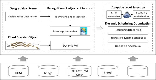
First, the basic geographic scenes based on multisource data fusion are constructed, and the flood spatiotemporal processes are simulated using cellular automata. Second, a dynamic identification method for objects of interest is designed, which based on the region of interest in multitime flood scenes. Finally, the error correction model and boundary optimization algorithm are designed to optimize the selection of multilevel scene objects. On this basis, a dynamic scheduling and queuing model with service interruption and dynamic priority is established to realize the adaptive optimization representation of the virtual scene of flood disasters.

2.2. ROI-constraints dynamic recognition of objects of interest

2.2.1. Data representation of flood scene objects

To ensure the integrity of flood disaster scenes, the scenes generally include basic geographic objects, disaster objects, disaster situation objects, emergency management objects, and secondary disaster objects (Li et al. 2020). Since geographic objects and disaster objects are the main sources of scene rendering pressure, this paper focuses on the rendering optimization methods for these two types of objects.

First, flood disasters involve a wide range of geographies, and geographic objects need to be organized and stored through data partitioning and pyramid model building. On the one hand, it facilitates data storage and dynamic loading. On the other hand, it facilitates multilevel adaptive expression of block data with ROI constraints to reduce the redundancy of scene data. Oblique photogrammetric data is used as a data source for geographic scene modelling in this article. Although it is used to represent three-dimensional real landscapes on the ground, it can still be stored using a two-dimensional data structure. On the other hand, region of interest recognition requires frequent calculations when floods are still ongoing, so recognition must be fast to ensure the efficiency of scene visualization. The rule blocking in the quadtree structure makes the detection of objects of interest faster and simpler. The rule blocking in the quadtree structure makes the detection of objects of interest faster and simpler, so regular quadtree is used for data organization, and some improvements are made. The accuracy of each node in the quadtree are extracted to build a Linear List and sorted, so that the level of detail can be found quickly according to viewpoint information. The basic unit of geographic object is represented as follows. (1) $Til{e}_{i,j}^{Lo{d}_{m,k}}=\{\mathrm{Data}\mathrm{Position},\mathrm{Accuracy},\mathrm{Bounding}\}.$(1) $Til{e}_{i,j}^{Lo{d}_{m,k}}$ represents the $k$th Level of Detail (LOD) Model of the $m$ layer of the ($i,j$) index block, and it is jointly represented by attributes such as centre position ($Position$), model accuracy ($Accuracy$) and bounding box ($Bounding$).

Second, as an important representation content of the disaster scene, the flood disaster object needs to be constructed from the aspects of its geometric structure, texture expression, spatiotemporal process, and attribute information. The cellular automata (CA) model can reveal the spatiotemporal complexity of flood disaster environments through repetitive simple calculations and has been proven to be simple and accurate in describing flow dynamics (Dottori and Todini 2011; Li et al. 2013; 2015, 2019; Parsons and Fonstad 2007; Rinaldi et al. 2007). Therefore, the cellular automata method is used to simulate flood evolution and construct a realistic flood representation model in this paper. The flood disaster object is represented as follows. (2) $Floo{d}_{t_i}=\{M,N,Size,Po{s}_0,\{deep(row,col)\}\}.$(2) $Floo{d}_{t_i}$ represents the flood simulation data at time $t_i$, which is represented by the number of rows ($M$), columns ($N$), grid size ($Size$), starting coordinates ($Po{s}_0$), and water depth values ($deep$) in the rows and columns ($row,col$).

2.2.2. Recognition of objects of interest in flood scenes

Considering that users mainly pay attention to the relevant scene objects within the flood disaster range when interacting with the scene, and pay less attention to the unaffected regions (Fu et al. 2021b), the inundation range of flood disasters at each moment is set as the boundary constraints of the region of interest. The specific steps of identifying the object of interest are as follows.

First, scene object spatial consistency processing is performed. Due to the different processing methods of multisource data, the direction and scale of the geographic object bounding box and the region of interest are inconsistent. Therefore, to simplify the spatial calculation process between the scene object and the region of interest, the surrounding circle of the scene object and the flood cells are used as the basic unit of calculation.

The second is the classification of interest types of scene objects. Spatial superposition analysis on the cell set of the submerged range of the flood evolution at each moment and the basic unit of the scene object is performed, and the type attribute of the basic unit of the scene object is obtained, as shown in Figure 2. The specific method is as follows.

Figure 2. Classification of interest types of scene objects.

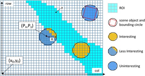
Calculate the range of the flood object grid in the scene object bounding circle, and set the local origin coordinates of the flood object as $(x_0,y_0)$, cell size as $a$, and scene object bounding circle as $C(p_x,p_{y}R)$, so the starting and ending column number can be represented as follows. (3) $\{\begin{array}{c}co{l}^{min}=Round\left({\displaystyle \frac{p_x-R-x_0}{a}}\right)\\ co{l}^{max}=Round\left({\displaystyle \frac{p_x+R-x_0}{a}}\right)\end{array}.$(3)

For each column, calculate the starting and ending row numbers. (4) $\{\begin{array}{c}ro{w}_i^{min}=Round\left({\displaystyle \frac{p_y-\sqrt{R^2-{(p_x-a\cdot i)}^2}-y_0}{a}}\right)\\ ro{w}_i^{max}=Round\left({\displaystyle \frac{p_y+\sqrt{R^2-{(p_x-a\cdot i)}^2}-y_0}{a}}\right)\end{array}.$(4)

Round () is the rounding function.

The total number of grids within the scene object bounding circle can be calculated as $M=\sum _{i=co{l}^{min}}^{co{l}^{max}}(ro{w}_i^{max}-ro{w}_i^{min})$, and the total number of grids within the inundation range can be calculated as $N=card(\{gri{d}_i|dee{p}_{gri{d}_i}⟩0\})$. Therefore, the type of interest of the scene object is shown in formula 5. (5) $Object=\{\begin{array}{c}Uninteresting,N=0\\ LessInteresting,0<N<M\\ Interesting,N=M\end{array}.$(5)

2.3. Flood scene representation optimization

2.3.1. Adaptive level selection optimization

Adaptive level selection has its own advantages in representation, which can optimize storage and improve the efficiency of on-demand visualization. For example, Hadimlioglu and King (2019) described a method for flood visualization using adaptive grids for position-based fluids method to visualize the depth of water.

1. Scene object level selection optimization with ROI constraints.

The screen projection error formula is used as the basis for level selection (Lindstrom et al. 1996; Zhang et al. 2017) to realize the preliminary multilevel expression of scene objects. The original digital surface model (DSM) collected is difficult to transmit, store, and visualize due to its high accuracy and wide range. Therefore, it is generally chunked and LOD simplification is applied to each data block. Different degrees of simplification in the simplification process lead to different geometric errors in the original data. The screen projection pixel error of the object can be calculated by formula (6), and then the value is compared with the given error threshold. If it is greater than this threshold then the current tile continues to the next level of subdivision, otherwise the current level is used for scene visualization. (6) $\rho ={\displaystyle \frac{L}{2\tan (\alpha /2)}\times {\displaystyle \frac{\delta }{D}.}}$(6) In practice, since users have different degrees of interest in different regions, the abovementioned level selection is still rough, and there is data redundancy. Therefore, further simplification is needed in combination with ROI. The spatial domain enhancement function T is constructed, and the enhancement or suppression of objects is realized by performing T transformation on ρ of different types of objects (Figure 3). (7) ${\rho }^{\mathrm{\prime }}=T\rho .$(7) The specific operations are as follows:

Figure 3. Schematic diagram of the error correction algorithm.

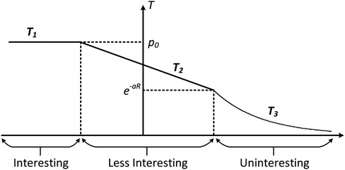
Since the data in the range of interest are strongly considered by users, it is necessary to enhance the objects of interest. Considering that the number of objects of interest is relatively small compared to the objects of noninterest, and the difference between them is small, the error correction factor of the objects of interest is uniformly set to the same constant $p_0$. (8) $T_1=p_0,p_0>1.$(8) For a human visual sensory stimulus, its behaviour follows the Weber-Fechner law, and the psychological quantity is a logarithmic function of the stimulus quantity (Sebastian, Abrams, and Geisler 2014). At the same time, the degree of interest in noninterested objects decreases as the distance of the remaining ROI increases. Therefore, the enhancement transformation function for noninterested objects is defined as follows. (9) $T_3=e^{-\alpha d},$(9) $d$ is the shortest distance between the scene object not of interest and the region of interest. $d>R$, and the adaptive adjustment parameter $\alpha >0$.

1. Boundary optimization based on visual continuity.

The initial level selection is based on the viewing distance, so the continuity of the level distribution of adjacent data can be guaranteed. However, after adding the spatial domain enhancement transformation function, the original continuity is destroyed, resulting in a level mutation at the boundary of the region of interest, and the visual continuity is destroyed. Therefore, it is necessary to smooth the mutation of details to optimize the boundary of the region of interest in the scene. The buffer zone is established with the object of weak interest in 2.2.2, and a linear transformation function is constructed with ${\displaystyle \frac{N}{M}}$ as the adjustment parameter of screen error. Then, hierarchical optimization of the scene objects at the boundary of the region of interest is performed to realize the visual continuity of the scene objects. As formula 10 shows. (10) $T_2=e^{-\alpha R}+(p_0-e^{-\alpha R})\ast {\displaystyle \frac{N}{M}.}$(10)

Figure 4. Flow chart of dynamic scheduling.

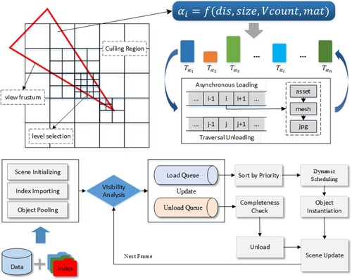
2.3.2 Dynamic scheduling optimization with service interruption

After the above tile-level optimization selection, the tile set that needs to be scheduled is obtained, and then the scheduling mechanism needs to be further optimized to improve the rendering efficiency of scene data. First, sort the tile sets that need to be scheduled to optimize the reasonable allocation of computer scheduling resources. Then, the data in the loading queue are judged in turn, and frame loading technology is used to realize the progressive loading of tile objects. Finally, an unloading mechanism considering the integrity of the scene is constructed to maintain the balance between the continuity of the system's visual effects and memory (Figure 4). The specific steps are as follows.

1. Rendering data sorting

There are different degrees of importance between the tile data blocks that fall into the viewing frustum. If only traversed block by block in a random way, it is very likely that the tile blocks with low interest are scheduled while those of interest have not yet started to update. Therefore, it is necessary to measure and sort the degree of interest of the visible tile block and preferentially load data blocks with high interest values.

From the summary of 2.3.1, the value of $T$ can be a good measure of the interest degree of scene objects. Therefore, $T$ is used as the basis for quantifying and sorting the importance of scene objects. The larger $T$ is, the higher the priority of dynamic scheduling of scene objects. The time cost of sorting is worth the better visual effect.

1. Progressive dynamic scheduling with service interruption

Add the selected optimized and sorted tiles to the current demand list $S_{new}$. Calculate the intersection and difference between the current demand list $S_{new}$ and the previous demand list $S_{old}$, the tile set $S^{+}$ to be loaded, the tile set $S^{-}$ to be unloaded, and the tile set $S^0$ that do not need to be processed are obtained. (11) $\{\begin{array}{c}{S}^{+}=\{s|s\in S_{new}\cap s\notin S_{old}\}\\ S^{-}=\{s|s\notin S_{new}\cap s\in S_{old}\}\\ S^0=\{s|s\in S_{new}\cap s\in S_{old}\}\end{array}.$(11) Different processing operations are taken for different types of sets.

1. For $S^{+}$, add it to the loading queue to judge whether it needs to be loaded;

2. For $S^{-}$, add it to the unloading queue to judge whether it needs to be unloaded;

3. For $S^0$, skip without any processing. This is because the time interval between frames is extremely short, and the set range of the current demand list $S_{new}$ and the previous demand list $S_{old}$ have not changed much. Under this condition, there are many elements in $S^0$, and skipping the calculation can effectively reduce computation.

The tile set $S^{+}$ that needs to be scheduled for each frame continuously enters the queue for queuing to receive services in turn; that is, the tile data are dynamically scheduled from the external memory to the memory and sent to the rendering pipeline for rendering. However, a queue that processes too long for each frame will cause the current frame to take too long to process, resulting in a drop-in frame rate. Therefore, to ensure the stability of the frame rate, the method of frame-by-frame loading, that is, progressive loading, is adopted.

A dynamic scheduling queuing model with service interruption and dynamic priority is applied in this paper for optimization. The length of the queue is controlled to be $N$, and only these $N$ pieces of data can be processed in each frame. $p_0$, $p_1$ … $p_n$ are set as the state parameters of the tile loading progress, only one phase of the task is completed per frame, and the loading of the frame is terminated after the loading progress of the data is recorded. Then, wait until the next frame continues loading according to the loading progress to ensure that the queue reorganization problems caused by changes in scene requirements can be responded to in time, as shown in $s_1$, $s_4$ and $s_{N-1}$ in Figure 6. In progressive loading, if the tile of the previous frame has not been loaded ($s_0$) or is being loaded but not completed ($s_2$) while the current frame needs to be unloaded, then terminate its loading progress in time and move it to the unloading queue. At the same time, the queue structure is dynamically adjusted, and the loading of newly added data that need to be scheduled is prioritized. The dynamic scheduling queuing model with service interruption and dynamic priority is shown in Figure 5.

1. Unloading mechanism that keeps the scene intact

Figure 5. Dynamic scheduling queuing model.

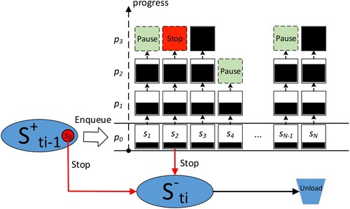
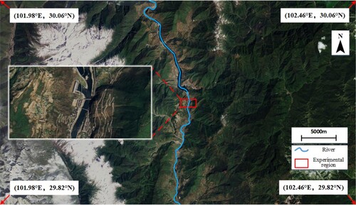
Figure 6. Experimental case region.

Due to the scheduling asymmetry caused by the real-time unloading and the delay of loading, the old scene is unloaded when the new scene is not loaded completely, and the scene representation is missing or flickering. Therefore, uninstallation can be performed only when the scene is judged to be complete. Whether the data are completely loaded can be quickly judged by the loading progress parameter $p_i$ set in 2.3.2, so it is only necessary to judge the integrity of each tile data in$S_{new}$, which represents the integrity of the scene tree. After the scene integrity is judged, the unloading process can be performed according to the current loading state of the data to ensure the correct release of the memory space.

3. Experimental analysis

3.1. Study area description

The case region selected in this paper is shown in Figure 6. The study area is located at the eastern edge of the Qinghai Tibet Plateau, and belongs to a typical mountain valley area. Excluding the non data portion (54.55%), the area is largely forested (41%), and a small part is covered in shrub and herbaceous associations (2.06%) and water bodies (0.98%). Urban fabric, industrial, commercial and transport units account for 0.66% of the region (https://osmlanduse.org/#13.41666666666667/102.2192/29.91687/0/). More than five earthquakes have occurred in the region in the past year, including a 6.8 magnitude earthquake on September 5, 2022. If water facilities such as reservoirs and embankments are damaged, it will cause flood disasters. In addition, the blockage of rivers by landslides and mudslides generated by earthquakes will lead to river diversions and overflows bringing flooding, or the formation of weirs, posing a potential threat.

The large-scale 3D reality model experimental data coverage is approximately 1.12 km², and the corresponding data blocks are managed by a total of 316 folders, occupying a total of 186 GB of disk space. First, the format conversion of the oblique photogrammetry model data is performed, and the original osgb data are converted into the obj three-dimensional format supported by unity. To alleviate the problem of slow parsing of the obj format when the system is dynamically scheduled, the grid data in the obj format are preprocessed into the AssetBundle format supported by Unity. At the same time, by calculating the attribute information of each tile offline, including location, size, precision and URL, an index file of tile data is constructed and stored in JSON format.

3.2. Prototype system development

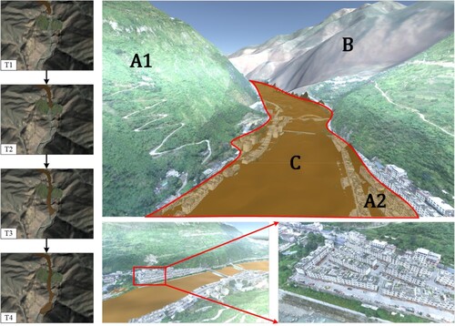
This paper chooses Microsoft Visual Studio 2017 and Unity 3D 2018 as the development environment, and the experiment is carried out with an Alienware m17 R4 laptop, the CPU is an Intel Core i7-10870H @2.2 GHz octa-core, the graphics card is an NVIDIA GeForce RTX 3080 laptop GPU, and the Windows10 operating system. A prototype system for interactive browsing of flood disaster scenes is developed, and the scene construction results of the prototype system are shown in Figure 7.

Figure 7. Flood disaster scene visualization prototype system interface. ($A_1$) Scene objects that are not in the area of interest. ($A_2$) Scene objects in the area of interest. ($B$) Basic terrain scene generated by DEM and images. ($C$) Flood disaster object.

3.3. Results analysis

3.3.1 Cognitive efficiency improvement analysis

To verify the effectiveness of the method in this paper, a questionnaire survey including three questions was conducted from the aspects of the real-life evaluation of user experience, the fluency of interactive exploration of scene roaming, and the content of attention to the scene, which is shown in Table 1. By experiencing the flood disaster visualization prototype system built in this paper, users score the first two questions. The score for each question is between 1 and 5 points. The higher the score is, the stronger the experience and the better the effect. The third question needs the user to answer which objects in the flood disaster scene are of interest after the experience.

Table 1. Questionnaire question design.

Type	Question	Score/Options
realization	Are you satisfied with the realism of the flood scene?	1. Very irreal 2. Irreal 3. Neutral 4. Real 5. Very real
Rendering efficiency	Do you think the flood scene is fluid?	1. Very rough 2. Rough 3. Neutral 4. Smooth 5. Very smooth
concern	Which objects in this flood scene do you primarily focus on?	1. Buildings affected 2. Flood 3. Depth of water 4. Terrain 5. Other

A total of 26 experiencers were convened, including 14 males and 12 females, ranging in age from 22 to 27 years old, all of whom had a bachelor's degree or above, and all had some understanding of 3D visualization of flood disasters. To avoid the influence of the experimental sequence on the results, the 26 experiencers were randomly divided into two groups, A and B. Group A first experienced the flood scene before optimization, and then experienced the flood scene optimized by the method in this paper, and the order of experience in group B was reversed. The experience time for each experiencer was 1 min, and the questionnaire was completed after the experience was completed. After the experiment, the average scores of the first two questions and the number of answer options for the last question were counted, as shown in Table 2.

Table 2. Comparative analysis of the average scores of the questionnaires.

Group	Q1(original /optimized)	Q2(original /optimized)	Q3
A	3.8/4.1	4.2/4.6	10/2/1/0/0
B	3.7/4.0	4.1/4.6	11/2/0/0/0

As seen from the above table, whether it is to experience the scene before optimization or the scene after optimization first, users always think that the optimized scene is more realistic, the visualization of the optimized flood scene is smoother, and the order of experiments had little effect on their perception of flood scenes. In addition, most of the experimenters expressed their interest in flooded buildings in the scene, and only a small number of users were interested in flood disaster information. They answered that the dynamic characteristics of the flood model attracted their attention, which also showed that users were more interested in the scenes within the flood range, and their focus was mainly on the inundation region of the flood disaster.

Using SPSS software (version 25), Mann-Whitney U-test was performed for two questions (q1 and q2) for Group A and Group B. The results of the four group tests showed that p (asymptotic significance) were less than 0.05. Therefore, the original hypothesis (no significant difference between experimental and control groups) was rejected and the experimental group could be considered as optimizing the control group.

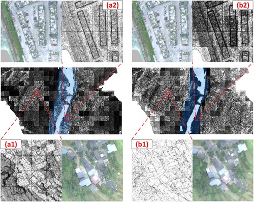
3.3.2 Rendering efficiency optimization analysis

To verify the feasibility of the method in this paper, qualitative and quantitative analysis methods are used for experimental verification. First, the flood scenes in the case area before optimization and after optimization using the method in this paper are qualitatively analysed. The experimental results are shown in Figure 8. (a1) and (a2) are the flood scenes before optimization, and (b1) and (b2) are the flood scenes after optimization. Compared with (a1) and (a2), it can be seen that the difference in the detailed expression of each area of the scene before optimization is small. Compared with (b1) and (b2), it is clear that the focus of the optimized scene detail expression is shifted to the region of interest. Comparing (a1) and (b1), it can be seen that the method in this paper simplifies the objects outside the region of interest. Compared with (a2) and (b2), it can be seen that the detailed expression of objects of interest to users within the flooded area is enhanced. The optimization method in this paper makes the distribution of the focus of the scene expression more hierarchical and more focused, which greatly reduces the redundant information in the scene.

Figure 8. Comparison of grid distribution and scene effects before and after optimization.

Second, the optimization effect of this method in flood scene representation is proven by quantitative analysis. First, the effect of ROI constraints is verified. To avoid the influence of the unstable dynamic scheduling process on the experimental analysis results, the average value of the number of triangles and the frame rate of the flood scene under three different static perspectives is calculated, as shown in Table 3. Due to the constraints of the region of interest, the number of scene triangles by the optimization method in this paper is reduced by approximately 30%, and the frame rate is increased by more than 15% due to the removal of a large amount of redundant scene data (Table 4).

Table 3. Mann – Whitney U before and after scene optimization.

Statistic hypothesis	Mann-Whitney U test	Wilcoxon rank-sum test	Z	p
A-q1	55	146	−2.202	0.28
A-q2	49.5	140.5	−2.046	0.41
B-q1	54	145	−2.281	0.23
B-q2	43	134	−2.454	0.14

Table 4. The effect of ROI on the number of triangles and frame rate in static scenes.

Angles of view	triangular surfaces		fps
	original	optimized	original	optimized
1	3.1 M	2.0 M	340	400
2	6.1 M	4.2 M	177	206
3	3.5 M	2.3 M	317	364

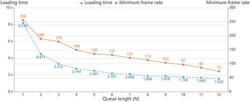
Next, the optimization effect of the dynamic scheduling strategy with service interruption is verified. To obtain appropriate queue length parameters, the relationship between scene loading time, minimum frame rate and queue length in a fixed viewing angle is calculated, as shown in Figure 9. As the queue length increases, the scene loading time and minimum frame rate continue to decrease. When the queue length $N$ exceeds 8, the loading time becomes stable and no longer decreases significantly. Therefore, to avoid freezing in scene visualization, the queue length parameter is set to 8 for the experiment, which does not make the loading time too long or the frame rate too low.

Figure 9. The relationship between scene loading time, frame rate and queue length.

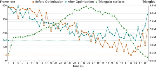
According to the composition characteristics of the scene data, the loading process is divided into four stages: loading the AB package ($p_1$), decompressing the AB package ($p_2$), instantiating the mesh objects ($p_3$), and adding the texture ($p_4$), and the service interruption mechanism is realized by Unity. Automatically roam along a fixed path at the same speed and count the changes in the frame rate and the number of triangular surfaces over time, as shown in Figure 10. As the number of triangles in the scene continues to increase, the frame rate gradually decreases. Although the scene data gradually decrease after 35 s, there are considerable objects that need to be updated in the scene, which makes the frame rate remain at a low level. It was not until after 55 s that the amount of data was reduced to a lower level that the frame rate picked up. More importantly, in the early stage of roaming, there is little difference in frame rate before and after optimization, and only after 39 s does it indicate that the frame rate after optimization is higher. To determine the reason, the change in the amount of new data in the scene over time was analysed. The results show that in the early stage of roaming, especially before 8 s, the frame rate before and after optimization is basically the same because the amount of newly added data is less. However, after 39s, the scene gradually becomes more complex, and the amount of newly added data is larger. In this case, the queue length is controlled by the dynamic scheduling optimization method of this paper so that the frame rate does not descend rapidly below 50 frames per second, similar to the unoptimized rate, but remains relatively stable above 148 frames per second. It can be seen that the rendering efficiency of the scene can be significantly improved by the optimization method of this paper.

Figure 10. Comparison of frame rates before and after optimization.

3.4 Discussion

The inundation range of flood disasters at each moment is set as the boundary constraints of the region of interest in this paper. This means that when the flood range is small, there are fewer refined data and more simplified data, resulting in a significant overall optimization effect. The advantage of this method is particularly prominent in flood visualization in high mountain canyon areas, as the shape of the flooded area is similar to a long strip, as shown in Figure 8. On the other hand, when the area of interest is large, the visualization lacks focus due to an increase in the amount of data that needs to be finely represented, such as in plain areas where the flood inundation range is large and extensive. Due to the complexity of the human visual system and visual tasks, the region of interest is often unable to be accurately determined. Therefore, further optimization should be considered to address the negative impact of changes in the scope of the region of interest.

The detailed representation could be also a key element for the generation of realistic 3D views able to enhance risk perception and communication (Costabile et al. 2021). The realistic scene was constructed using high-precision DSM data obtained from photogrammetry in this paper, as well as using cellular automata to simulate the flood evolution process offline, achieving enhanced expression of flood risk. However, it still lacks detailed consideration of the visualization effect of flood expression in this paper, as during reconstruction, discretization and interpolation artefacts can occur, including water climbing uphill, sinking into the ground, etc., which is considered misleading and unaesthetic (Cornel et al. 2019).

Geohazard research requires extensive spatiotemporal understanding based on an adequate multi-scale representation of modelling results (Havenith, Cerfontaine, and Mreyen 2019). VR technology could create 3D real-world environments and provide an attractive solution to overcome the multi-dimensional and spatiotemporal obstacles (Sermet and Demir 2022). Similarly, with the development of extended reality technology in recent years, the perception of geographic information has been widely improved. In this paper, the focus of scene representation is shifted to the region of interest by enhancing the content of interest and simplifying the content of non-interest. The method is suitable for universal 3D geographic scene visualization and can provide a theoretical basis for other related research.

4. Conclusions and future work

This research article presents a ROI-constrained visualization method of flood scenes to improve perception efficiency. A dynamic recognition method of flood scene ROIs is proposed based on the characteristics of the flood evolution process, which can avoid the interference of complex background to improve the processing efficiency, because the attention will be quickly attracted by several salient objects. A multi-level scene object selection and dynamic scheduling method with service interruption is designed to optimize the representation of flood disaster scenes adaptively. The method adaptively acquires large-scale flood scene ROIs and dynamically optimizes reorganization of rendering queues, which reduces the computational redundancy of dynamic data scheduling and overload of scene information representation. Experimental results show that approximately 30% of the redundant data are reduced, and the scene rendering efficiency is increased by approximately 15%. The non-ROI visualization is weakened by using the rules of human visual cognition, which improves the perception efficiency of flood scenes. The main contributions of this paper are summarized as follows.

First, the selective filtering feature of human visual system is used to enhance the expression of flood scene. The ROI recognition method is proposed to filter the key objects in the scene to distinguish the level of expression details of different objects. Then the hierarchical selection and boundary optimization algorithm is constructed, which considers visual continuity, which can reduce redundant data and improve user perception efficiency.

Second, the adaptive dynamic scheduling algorithm is designed to better support the stable update and efficient rendering of flood scenes. A dynamic scheduling queuing model with service interruption is designed, which can quickly optimize and adjust the rendering queue structure by listening for changing update requests, so as to achieve stable update of flood scenes. The algorithm can alleviate the problem of massive and high-precision flood scene rendering stagnation during interactive browsing, and help to improve user experience and the efficiency of geographic information expression.

However, there are still some shortcomings in this paper. For example, this paper only optimizes high-precision basic geographic objects and does not consider the optimization of other disaster information in flood disaster scenes. In addition, Accurate ROI recognition is expected to further improve frame rate. The inundation range of flood disasters at each moment is set as the boundary constraints of the region of interest in this paper. For larger regions of interest, the visualization is no longer focused due to the increasing amount of data that needs to be finely represented. Due to the complexity of the human visual system and visual tasks, the region of interest is often unable to be accurately determined. The experimental results may be further enhanced if the region of interest can be accurately acquired in real time, for example, by in-depth analysis and utilization of the eye-movement data acquired by the eye-tracking device (Liao et al. 2019). Therefore, in the follow-up research work, we will combine the relevant theories of cognitive psychology to optimize the visual representation of the whole process and all elements of the flood disaster scene, further improve the theoretical framework of the visualization of the virtual flood disaster scene, and provide a comprehensive and effective solution for flood disaster management.

Data availability statement

The data presented in this study are available on request from the corresponding author.

Disclosure statement

No potential conflict of interest was reported by the author(s).

Additional information

Funding

This paper was funded by National Natural Science Foundation of China [grant number U2034202, 42271424 and 41871289].

References

- Andújar, C., C. S. Vázquez, and I. Navazo. 2000. “LOD Visibility Culling and Occluder Synthesis.” Computer-Aided Design 32 (13): 773–783. https://doi.org/10.1016/S0010-4485(00)00067-1.
- Biljecki, F., H. Ledoux, and J. Stoter. 2017. “Generating 3D City Models Without Elevation Data.” Computers, Environment and Urban Systems 64: 1–18. https://doi.org/10.1016/j.compenvurbsys.2017.01.001.
- Bittner, K., P. d’Angelo, M. Körner, and P. Reinartz. 2018. “DSM-to-LoD2: Spaceborne Stereo Digital Surface Model Refinement.” Remote Sensing 10 (12): 1926. https://doi.org/10.3390/rs10121926.
- Bshouty, E., A. Shafir, and S. Dalyot. 2020. “Towards the Generation of 3D OpenStreetMap Building Models from Single Contributed Photographs.” Computers, Environment and Urban Systems 79: 101421. https://doi.org/10.1016/j.compenvurbsys.2019.101421.
- Carrasco, M. 2011. “Visual Attention: The Past 25 Years.” Vision Research 51 (13): 1484–1525. https://doi.org/10.1016/j.visres.2011.04.012.
- Chen, Q., G. Liu, X. Ma, G. Mariethoz, Z. He, Y. Tian, and Z. Weng. 2018. “Local Curvature Entropy-Based 3D Terrain Representation Using a Comprehensive Quadtree.” ISPRS Journal of Photogrammetry and Remote Sensing 139: 30–45. https://doi.org/10.1016/j.isprsjprs.2018.03.001.
- Cheng, G. C., and B. Buckles. 2014. “A Nonparametric Approach to Region-of-Interest Detection in Wide-Angle Views.” Pattern Recognition Letters 49 (1): 24–32. https://doi.org/10.1016/j.patrec.2014.05.019.
- Cornel, D., A. Buttinger-Kreuzhuber, A. Konev, Z. Horváth, M. Wimmer, R. Heidrich, and J. Waser. 2019. “Interactive Visualization of Flood and Heavy Rain Simulations.” Computer Graphics Forum 38 (3): 25–39. https://doi.org/10.1111/cgf.13669.
- Costabile, P., C. Costanzo, G. De Lorenzo, R. De Santis, N. Penna, and F. Macchione. 2021. “Terrestrial and Airborne Laser Scanning and 2-D Modelling for 3-D Flood Hazard Maps in Urban Areas: New Opportunities and Perspectives.” Environmental Modelling & Software 135: 104889. https://doi.org/10.1016/j.envsoft.2020.104889.
- Dottori, F., and E. Todini. 2011. “Developments of a Flood Inundation Model Based on the Cellular Automata Approach: Testing Different Methods to Improve Model Performance.” Physics and Chemistry of the Earth, Parts A/B/C 36 (7): 266–280. https://doi.org/10.1016/j.pce.2011.02.004.
- Feng, Y., Q. Xiao, C. Brenner, A. Peche, J. Yang, U. Feuerhake, and M. Sester. 2022. “Determination of Building Flood Risk Maps from LiDAR Mobile Mapping Data.” Computers, Environment and Urban Systems 93: 101759. https://doi.org/10.1016/j.compenvurbsys.2022.101759.
- Fu, H., H. Yang, and C. Chen. 2021a. “Large-scale Terrain-Adaptive LOD Control Based on GPU Tessellation.” Alexandria Engineering Journal 60 (3): 2865–2874. https://doi.org/10.1016/j.aej.2021.01.029.
- Fu, L., J. Zhu, W. L. Li, Q. Zhu, B. L. Xu, Y. K. Xie, Y. H. Zhang, et al. 2021b. “Tunnel Vision Optimization Method for VR Flood Scenes Based on Gaussian Blur.” International Journal of Digital Earth 14 (7): 821–835. https://doi.org/10.1080/17538947.2021.1886359.
- Hadimlioglu, I. A., and S. A. King. 2019. “Visualization of Flooding Using Adaptive Spatial Resolution.” ISPRS International Journal of Geo-Information 8 (5): 204. https://doi.org/10.3390/ijgi8050204.
- Havenith, H. B., P. Cerfontaine, and A. S. Mreyen. 2019. “How Virtual Reality Can Help Visualise and Assess Geohazards.” International Journal of Digital Earth 12 (2): 173–189. https://doi.org/10.1080/17538947.2017.1365960.
- Haynes, P., S. Hehl-Lange, and E. Lange. 2018. “Mobile Augmented Reality for Flood Visualisation.” Environmental Modelling & Software 109: 380–389. https://doi.org/10.1016/j.envsoft.2018.05.012.
- Hernández, D., J. M. Cecilia, J. C. Cano, and C. T. Calafate. 2022. “Flood Detection Using Real-Time Image Segmentation from Unmanned Aerial Vehicles on Edge-Computing Platform.” Remote Sensing 14 (1): 223. https://doi.org/10.3390/rs14010223.
- Hu, Y., J. Zhu, W. L. Li, Y. H. Zhang, M. Y. Hu, and Z. Y. Cao. 2018. “A Construction Optimization and Interaction Method for Flood Disaster Scenes Based on Mobile VR.” Acta Geodaetica et Cartographica Sinica 47 (08): 1123–1132. https://doi.org/10.11947/j.AGCS.2018.20180114.
- Huang, W. M., J. Chen, and M. Y. Zhou. 2020. “A Binocular Parallel Rendering Method for VR Globes.” International Journal of Digital Earth 13 (9): 998–1016. https://doi.org/10.1080/17538947.2019.1620883.
- Li, W., and P. Dong. 2013. “Object Recognition Based on the Region of Interest and Optical bag of Words Model.” In Proceedings of the Fifth International Conference on Internet Multimedia Computing and Service, 394–398. https://doi.org/10.1145/2499788.2499873.
- Li, Y., J. Gong, H. Liu, J. Zhu, Y. Song, and J. Liang. 2015. “Real-time Flood Simulations Using CA Model Driven by Dynamic Observation Data.” International Journal of Geographical Information Science 29 (4): 523–535. https://doi.org/10.1080/13658816.2014.977292.
- Li, Y., J. Gong, J. Zhu, Y. Song, Y. Hu, and L. Ye. 2013. “Spatiotemporal Simulation and Risk Analysis of dam-Break Flooding Based on Cellular Automata.” International Journal of Geographical Information Science 27 (10): 2043–2059. https://doi.org/10.1080/13658816.2013.786081.
- Li, Y., B. Hu, D. Zhang, J. Gong, Y. Song, and J. Sun. 2019. “Flood Evacuation Simulations Using Cellular Automata and Multiagent Systems -a Human-Environment Relationship Perspective.” International Journal of Geographical Information Science 33 (11): 2241–2258. https://doi.org/10.1080/13658816.2019.1622015.
- Li, M. L., and L. L. Nan. 2021. “Feature-preserving 3D Mesh Simplification for Urban Buildings.” ISPRS Journal of Photogrammetry and Remote Sensing 173: 135–150. https://doi.org/10.1016/j.isprsjprs.2021.01.006.
- Li, S., C. Zheng, R. Wang, Y. Huo, W. Zheng, H. Lin, and H. Bao. 2021a. “Multi-resolution Terrain Rendering Using Summed-Area Tables.” Computers & Graphics 95: 130–140. https://doi.org/10.1016/j.cag.2021.02.003.
- Li, W., J. Zhu, P. Dang, J. Wu, J. Zhang, L. Fu, and Q. Zhu. 2023. “Immersive Virtual Reality as a Tool to Improve Bridge Teaching Communication.” Expert Systems with Applications 217: 119502. https://doi.org/10.1016/j.eswa.2023.119502.
- Li, W., J. Zhu, L. Fu, Q. Zhu, Y. Guo, and Y. Gong. 2021b. “A Rapid 3D Reproduction System of dam-Break Floods Constrained by Post-Disaster Information.” Environmental Modelling & Software 139: 104994. https://doi.org/10.1016/j.envsoft.2021.104994.
- Li, W., J. Zhu, L. Fu, Q. Zhu, Y. Xie, and Y. Hu. 2020. “An Augmented Representation Method of Debris Flow Scenes to Improve Public Perception.” International Journal of Geographical Information Science 35 (8): 1521–1544. https://doi.org/10.1080/13658816.2020.1833016.
- Li, W., J. Zhu, Y. Gong, Q. Zhu, B. Xu, and M. Chen. 2022a. “An Optimal Selection Method for Debris Flow Scene Symbols Considering Public Cognition Differences.” International Journal of Disaster Risk Reduction 168 (102698): 1–12. https://doi.org/10.1016/j.ijdrr.2021.102698.
- Li, W., J. Zhu, S. Pirasteh, Q. Zhu, L. Fu, J. Wu, Y. Hu, and Y. Dehbi. 2022b. “Investigations of Disaster Information Representation from a Geospatial Perspective: Progress, Challenges and Recommendations.” Transactions in GIS 26 (3): 1376–1398. https://doi.org/10.1111/tgis.12922.
- Liao, H., W. Dong, H. Huang, G. Gartner, and H. Liu. 2019. “Inferring User Tasks in Pedestrian Navigation from eye Movement Data in Real-World Environments.” International Journal of Geographical Information Science 33 (4): 739–763. https://doi.org/10.1080/13658816.2018.1482554.
- Lim, N. J., S. A. Brandt, and S. Seipel. 2015. “Visualisation and Evaluation of Flood Uncertainties Based on Ensemble Modelling.” International Journal of Geographical Information Science 30 (2): 240–262. https://doi.org/10.1080/13658816.2015.1085539.
- Lindstrom, P., D. Koller, W. Ribarsky, L. F. Hodges, N. Faust, and G. A. Turner. 1996. “Real-time, continuous level of detail rendering of height fields.” Proceedings of the 23rd annual conference on Computer graphics and interactive techniques 109–118. doi: 10.1145/237170.237217.
- Liu, M., J. Zhu, Q. Zhu, H. Qi, L. Yin, X. Zhang, B. Feng, H. He, W. Yang, and L. Chen. 2017. “Optimization of Simulation and Visualization Analysis of dam-Failure Flood Disaster for Diverse Computing Systems.” International Journal of Geographical Information Science 31 (9): 1891–1906. https://doi.org/10.1080/13658816.2017.1334897.
- Mai, T., S. Mushtaq, K. Reardon-Smith, P. Webb, R. Stone, J. Kath, and D. A. An-Vo. 2020. “Defining Flood Risk Management Strategies: A Systems Approach.” International Journal of Disaster Risk Reduction 47: 101550. https://doi.org/10.1016/j.ijdrr.2020.101550.
- Mao, B., L. Harrie, and Y. Ban. 2012. “Detection and Typification of Linear Structures for Dynamic Visualization of 3D City Models.” Computers, Environment and Urban Systems 36 (3): 233–244. https://doi.org/10.1016/j.compenvurbsys.2011.10.001.
- Minano, A., J. Thistlethwaite, D. Henstra, and D. Scott. 2021. “Governance of Flood Risk Data: A Comparative Analysis of Government and Insurance Geospatial Data for Identifying Properties at Risk of Flood.” Computers, Environment and Urban Systems 88: 101636. https://doi.org/10.1016/j.compenvurbsys.2021.101636.
- Nouvel, R., M. Zirak, V. Coors, and U. Eicker. 2017. “The Influence of Data Quality on Urban Heating Demand Modeling Using 3D City Models.” Computers, Environment and Urban Systems 64: 68–80. https://doi.org/10.1016/j.compenvurbsys.2016.12.005.
- Parsons, J. A., and M. A. Fonstad. 2007. “A Cellular Automata Model of Surface Water Flow.” Hydrological Processes 21 (16): 2189–2195. https://doi.org/10.1002/(ISSN)1099-1085.
- Peden, A. E., A. Mayhew, and S. D. Baker. 2022. “Experiences, Beliefs, and Attitudes of Lifeguards from Australia and the United Kingdom Toward Lifeguard Involvement in Flood Mitigation and Response.” International Journal of Disaster Risk Reduction 76: 103013. https://doi.org/10.1016/j.ijdrr.2022.103013.
- Pugliese, F., G. Caroppi, A. Zingraff-Hamed, G. Lupp, and C. Gerundo. 2022. “Assessment of NBSs Effectiveness for Flood Risk Management: The Isar River Case Study.” Journal of Water Supply: Research and Technology-Aqua 71 (1): 42–61. https://doi.org/10.2166/aqua.2021.101.
- Rinaldi, P. R., D. D. Dalponte, M. J. Vénere, and A. Clausse. 2007. “Cellular Automata Algorithm for Simulation of Surface Flows in Large Plains.” Simulation Modelling Practice and Theory 15 (3): 315–327. https://doi.org/10.1016/j.simpat.2006.11.003.
- Romero, T. Q., and J. Leandro. 2022. “A Method to Devise Multiple Model Structures for Urban Flood Inundation Uncertainty.” Journal of Hydrology 604: 127246. https://doi.org/10.1016/j.jhydrol.2021.127246.
- Saligrama, V., J. Konrad, and P. M. Jodoin. 2010. “Video Anomaly Identification.” IEEE Signal Process Magazine 27 (5): 18–33. https://doi.org/10.1109/MSP.2010.937393.
- Schröter, K., M. Barendrecht, M. Bertola, A. Ciullo, R. T. da Costa, L. Cumiskey, A. Curran, et al. 2021. “Large-scale Flood Risk Assessment and Management: Prospects of a Systems Approach.” Water Security 14: 100109. https://doi.org/10.1016/j.wasec.2021.100109.
- Sebastian, S., J. Abrams, and W. S. Geisler. 2014. “Measuring the Laws of Natural Vision by Constrained Natural Scene Sampling.” Journal of Vision 14 (10): 647. https://doi.org/10.1167/14.10.647.
- Seipel, S., and N. J. Lim. 2017. “Color map Design for Visualization in Flood Risk Assessment.” International Journal of Geographical Information Science 31 (11): 2286–2309. https://doi.org/10.1080/13658816.2017.1349318.
- Sermet, Y., and I. Demir. 2022. “Geospatial VR: A web-Based Virtual Reality Framework for Collaborative Environmental Simulations.” Computers & Geosciences 159: 105010. https://doi.org/10.1016/j.cageo.2021.105010.
- She, J., Y. Zhou, X. Tan, X. Li, and X. Guo. 2017. “A Parallelized Screen-Based Method for Rendering Polylines and Polygons on Terrain Surfaces.” Computers & Geosciences 99: 19–27. https://doi.org/10.1016/j.cageo.2016.10.011.
- Song, Z. Y., and J. Li. 2018. “A Dynamic Tiles Loading and Scheduling Strategy for Massive Oblique Photogrammetry Models.” 2018 IEEE 3rd International Conference on Image, Vision and Computing (ICIVC), 648–652. https://doi.org/10.1109/ICIVC.2018.8492731.
- Spero, H. R., I. Vazquez-Lopez, K. Miller, R. Joshaghani, S. Cutchin, and J. Enterkine. 2022. “Drones, Virtual Reality, and Modeling: Communicating Catastrophic dam Failure.” International Journal of Digital Earth 15 (1): 585–605. https://doi.org/10.1080/17538947.2022.2041116.
- Tierolf, L., D. H. Moel, and J. V. Vliet. 2021. “Modeling Urban Development and its Exposure to River Flood Risk in Southeast Asia.” Computers, Environment and Urban Systems 87: 101620. https://doi.org/10.1016/j.compenvurbsys.2021.101620.
- Totschnig, R. and Fuchs, S., 2013. Mountain Torrents: Quantifying Vulnerability and Assessing Uncertainties.” Engineering Geology 155: 31–44. https://doi.org/10.1016/j.enggeo.2012.12.019.
- Wilkinson, M. E., E. Mackay, P. F. Quinn, M. Stutter, K. J. Beven, C. J. Macleod, M. G. Macklin, et al. 2015. “A Cloud Based Tool for Knowledge Exchange on Local Scale Flood Risk.” Journal of Environmental Management 161: 38–50. https://doi.org/10.1016/j.jenvman.2015.06.009.
- Xie, Y., J. Zhu, J. Lai, P. Wang, D. Feng, Y. Cao, T. Hussain, and S. Baik. 2022. “An Enhanced Relation-Aware Global-Local Attention Network for Escaping Human Detection in Indoor Smoke Scenarios.” ISPRS Journal of Photogrammetry and Remote Sensing 186: 140–156. https://doi.org/10.1016/j.isprsjprs.2022.02.006.
- Yao, C., G. Peng, Y. Song, and M. Duan. 2017. “A Quadtree Organization Construction and Scheduling Method for Urban 3d Model Based on Weight.” ISPRS - International Archives of the Photogrammetry, Remote Sensing and Spatial Information Sciences 42: 977–980. https://doi.org/10.5194/isprs-archives-XLII-2-W7-977-2017.
- Yılmaz, T., and U. Güdükbay. 2007. “Conservative Occlusion Culling for Urban Visualization Using a Slice-Wise Data Structure.” Graphical Models 69 (3): 191–210. https://doi.org/10.1016/j.gmod.2007.01.002.
- Zhang, G., J. Gong, Y. Li, J. Sun, B. Xu, D. Zhang, J. Zhou, L. Guo, S. Shen, and B. Yin. 2020b. “An Efficient Flood Dynamic Visualization Approach Based on 3D Printing and Augmented Reality.” International Journal of Digital Earth 13 (11): 1302–1320. https://doi.org/10.1080/17538947.2019.1711210.
- Zhang, H., X. Guo, D. Wang, and J. Jia. 2020c. “Preloading Mechanism of Large-Scale Web3D Scene Based on DR Prediction.” Journal of System Simulation 32 (07): 1341–1348. https://doi.org/10.16182/j.issn1004731x.joss.19-vr0469.
- Zhang, K., M. H. Shalehy, G. T. Ezaz, A. Chakraborty, K. M. Mohib, and L. Liu. 2022. “An Integrated Flood Risk Assessment Approach Based on Coupled Hydrological-Hydraulic Modeling and Bottom-up Hazard Vulnerability Analysis.” Environmental Modelling & Software 148: 105279. https://doi.org/10.1016/j.envsoft.2021.105279.
- Zhang, F., Q. Wei, and L. Xu. 2020a. “An Fast Simulation Tool for Fluid Animation in VR Application Based on GPUs.” Multimedia Tools and Applications 79: 16683–16706. https://doi.org/10.1007/s11042-019-08002-4.
- Zhang, Y. H., Q. Zhu, J. Zhu, M. W. Liu, H. G. He, W. J. Yang, P. C. Zhang, and Z. Y. Cao. 2017. “Lightweight Web Visualization of Massive DSM Data.” Journal of Geomatics Science and Technology 34 (06): 649–653. https://doi.org/10.3969/j.issn.1673-6338.2017.06.020.
- Zhang, Y. H., J. Zhu, Q. Zhu, Y. K. Xie, W. L. Li, L. Fu, J. X. Zhang, and J. M. Tan. 2020d. “The Construction of Personalized Virtual Landslide Disaster Environments Based on Knowledge Graphs and Deep Neural Networks.” International Journal of Digital Earth 13 (12): 1637–1655. https://doi.org/10.1080/17538947.2020.1773950.
- Zhuo, L., and D. Han. 2020. “Agent-based Modelling and Flood Risk Management: A Compendious Literature Review.” Journal of Hydrology 591: 125600. https://doi.org/10.1016/j.jhydrol.2020.125600.