Space-associated domain adaptation for three-dimensional mineral prospectivity modeling

ABSTRACT

Geographical information systems (GIS) are essential tools for mineral prospectivity modeling (MPM). Three-dimensional (3D) MPM is able to learn the association between geological evidence and mineralization in shallow zones and thereby build a prospectivity model for deep zones, making it a desirable technique to target deep-seated orebodies. However, existing 3D MPM methods directly generalize the model learned in shallow zones to the deep zones without attention to model transferability caused by the different metallogenic mechanisms between the two zones. In this study, we aim to robustly transfer the prospectivity model learned from shallow zones to deep zones. We cast the 3D MPM as a domain adaptation problem, which is an important realm of transfer learning. Because the metallogenic mechanism can be closely associated with spatial locations, we specifically focus on domain adaption concerning the spatial locations that are ignored by conventional domain adaptation methods. To measure the spatial-associated domain discrepancy, we propose a novel spatial-associated maximum mean discrepancy (SAMMD), which compares the joint distributions of features and spatial locations across domains. Based on the SAMMD criterion, a deep neural network, referred to as the spatial-associated domain adaptation network, is devised to learn cross-domain but mineralization-indicative features for building prospectivity model that is transferable to deep zones. A case study of the world-class Sanshandao gold deposit, in eastern China, was carried out to validate the effectiveness of the proposed methods. The results show that compared with other leading MPM methods and other domain adaption variants, the proposed method has superior prediction accuracy and targeting efficiency, demonstrating the effectiveness and robustness of the proposed method in targeting deep-seated orebodies in areas with different metallogenic mechanisms and no labeled data.

KEYWORDS:

• Mineral prospectivity modeling
• domain adaptation
• spatial factor
• feature dissimilarity
• kernel learning

1. Introduction

Geographical information systems (GIS) have been widely applied in mineral prospectivity modeling (MPM) (Bonham-Carter 1994; Carranza 2008; Rodriguez-Galiano et al. 2014, 2015). Owing to a powerful ability to acquire, store, process, analyze, and visualize spatial data, GIS workflows are capable of collecting multi-source/scale geosciences data, representing geological objects and evidence, analyzing the geoscientific information, modeling the association to mineralizations, and predicting mineral exploration targets in the MPM task. With the advances of three-dimensional (3D) GIS, especially 3D modeling and 3D spatial analysis techniques, GIS-based 3D MPM has emerged (Deng et al. 2022; Fallara, Legault, and Olivier 2006; Li et al. 2015, 2019; Mao et al. 2019; Wang et al. 2015, 2011; Xiao et al. 2015; Yuan et al. 2014). GIS-based 3D MPM has recently become a desirable technique for visualization and quantitative targeting of deep-seated mineralization.

GIS-based mineral prospectivity methods can be categorized into two groups: data-driven and knowledge-driven. Knowledge-driven models use subjective evidence based on prior knowledge of processes that may contribute to the formation of mineral deposits under circumstances where few mineral deposits are known to occur (Carranza 2008). On the other hand, data-driven models can be built with less subjective knowledge of geological settings and mineral deposits (Bonham-Carter 1994). Due to the emergence of geosciences data in this big-data era and demand for reduced dependence on subjective experience, data-driven prospectivity methods have become the advocated paradigm in MPM (Carranza and Laborte 2015a, 2015b; McKay and Harris 2016; Xiong and Zuo 2018; Yousefi and Nykänen 2016).

Conventionally, multivariate analysis has been used to find associations between predictor variables and mineralization. However, due to the complicated mineralization processes, associations between geological evidence and mineralization are very complex. Therefore, the machine learning approach is a promising category of data-driven methods to model the complex associations of mineralization. Mainstream machine learning approaches such as support vector machines (Zuo and Carranza 2011), random forests (Carranza and Laborte 2015b; Rodriguez-Galiano et al. 2014, 2015), artificial neural networks (Brown et al. 2000; Chen 2015; Chen and Wu 2017), and ensemble approaches (Wang et al. 2020) are utilized to integrate multi-source geoinformation and build mineral prospectivity models. Recently, deep learning-based methods have been applied to MPM because they can automatically extract high-level representations directly from data (Zuo 2020; Zuo et al. 2021). A series of advances have evolved mainly in 2D MPM (Li, Qian, and Li 2020; Li et al. 2021; Xiong and Zuo 2018, 2020, 2021; Yang et al. 2021; Zhang et al. 2021). Despite starting relatively late in 3D MPM, Li et al. (2021) first adopted 3D convolutional neural networks (CNN) to learn the 3D evidence layers and extract high-level features. Deng et al. (2022) proposed a 2D CNN method that directly learns high-level features from primitive shape descriptors of 3D geological models. These deep learning methods have achieved outstanding performance in predicting exploration targets.

The specific task of 3D MPMs is to predict the 3D distribution of mineral prospectivity and identify mineralization targets in deep-seated zones. While machine-learning methods have been shown to be effective in the predictive mapping of mineral prospectivity, modeling of mineral prospectivity in deep-seated zones is rather challenging. Due to the differences in temperature, pressure, and rock permeability at different positions, the characteristics of tectonic stress, fluid transport, and mineral localization mechanisms can be different between shallow and deep zones. With increasing prospective depths, such differences would become more significant, consistent with Tobler's first law of geography: ‘Near things are more related than distant things (Tobler 1970, 2004)’. Additionally, because of the limited exploration depth and the high cost of data acquisition, the geoinformation related to deep-seated zones is generally highly scarce, uncertain and heterogeneous. Directly generalizing the mineralization information captured from shallow zones limits the effectiveness of mineral prospectivity models in deep zones (Cloetingh and Podladchikov 2000). However, existing 3D MPM methods predict mineral prospectivity in deep zones by directly learning and generalizing mineral associations from shallow zones. The differences in metallogenic mechanism and the information discrepancy between the two zones are not typically emphasized.

From a machine learning perspective, 3D MPM targeting deep-seated economic orebodies can be regarded as a domain adaptation problem, an important subcategory of transfer learning (Pan and Yang 2009; Weiss, Khoshgoftaar, and Wang 2016; Zhuang et al. 2020). Domain adaptation seeks to enhance the performance of a target model with inadequate or no labeled data by transferring the features learned from a source domain with sufficient labeled data. The major goal of domain adaptation is to narrow the gap across domains, thereby guaranteeing model performance. A discrepancy-based mechanism is commonly applied to bridge the gap between source and target domains through a latent feature space (Ding and Fu 2017; Gong, Grauman, and Sha 2013; Long et al. 2014; Pan et al. 2011; Sun, Feng, and Saenko 2015; Wang et al. 2018; Zhang, Li, and Ogunbona 2017; Zhang et al. 2013). Recent advances in deep learning shows that deep neural networks ensure domain adaptation models to learn more transferable features (Bousmalis et al. 2016; Long et al. 2015, 2016, 2017; Tzeng et al. 2014; Yan et al. 2017; Zhang et al. 2015). For 3D MDM scenario, the shallow zones generally include adequate labeled data, and thus can be regarded as the source domain in domain adaptation. In contrast, the deep zones, whose metallogenic mechanism are probably different, are endowed and with limited or even no labeled data, and thereby correspond to the target domain. Therefore, 3D MPM can be regarded as a typical domain adaptation task. By casting 3D MPM as a domain adaptation problem, it is expected to bridge the discrepancy of metallogenic mechanism and mineralization information between shallow and deep zones.

Even though domain adaptation is reasonable for 3D MPM scenarios, introducing the domain adaptation paradigm to model mineral prospectivity is non-trivial. The spatial variance of metallogenic mechanism follows Tobler's first law of geography, wherein the metallogenic mechanism in deep zones is correlated to that in shallow zones (Tobler 1970, 2004), but the mechanism at nearby locations is more correlated than the distant ones. This suggests that the domain discrepancy in 3D MPM is essentially associated with spatial locations, making the spatial location a determinant in domain adaptation. Existing domain adaptation methods were originally designed for problems involving, for example, images, videos, or text for applications in computer vision and natural language processing. These methods only estimate the domain discrepancy according to the feature discrepancy. To the best of our knowledge, none of them has considered the domain discrepancy across the geographical space and used spatial locations to estimate feature transferability for domain adaptation.

In this study, we introduce a transfer learning paradigm to 3D MPM and present a spatial-associated domain adaptation method for building mineral prospecivity models. Specifically, the spatial-associated maximum mean discrepancy (SAMMD) is derived, which measures kernel mean embedding of the joint distributions of features and spatial locations and enables the estimation of the domain discrepancy over geospace. Using SAMMD, a spatial-associated domain adaptation network is developed, which incorporates SAMMD as the domain adaptation module to the top layers of a convolution neural network (CNN). The network learns mineralization-associated and transferable features across geospace by minimizing the fitness to source data (shallow zones) and the SAMMD between source and target domains (deep zones). The 3D mineral prospectivity model evolves and is developed based on the network. A case study investigating the Sanshandao gold deposit in eastern China demonstrates that the proposed method achieves outstanding results regarding prediction accuracy and target efficiency.

2. Methodology

2.1. Problem definitions

For a domain adaptation problem in the 3D MPM scenario, we are given a source domain (i.e. shallow zones) of m labeled data $(X^s,Y^s):=\left\{\right(x_1^s,y_1^s),\dots ,(x_m^s,y_m^s\left)\right\}$, where $x_i^s$ and $y_i^s$ denote the features and the ore-bearing label in the source domain, respectively, and the target domain (i.e. deep zones) of n unlabeled data $X^t:=\{x_1^t,\dots ,x_n^t\}$, where $x_i^t$ denotes the observed features in the target domain. Each source domain and target domain data is associated with the spatial location $Z^s:=\{z_1^s,\dots ,z_m^s\}$ and $Z^t:=\{z_1^t,\dots ,z_n^t\}$ in source and target domains, respectively. The source and target domain data are represented as marginal distributions $P\left(X^s\right)$ and $Q\left(X^t\right)$, joint distributions $P(X^s,Y^s)$ and $Q(X^t,Y^t)$, and conditional distributions $P\left(Y^s\right|X^s)$ and $Q\left(Y^t\right|X^t)$, where $Y^t$ represents the predicted ore-bearing label in the target domain. Due to the different metallogenic mechanism between source and target domains, we assume $P\left(X^s\right)\ne Q\left(X^t\right)$, $P(X^s,Z^s)\ne Q(X^t,Z^t)$ and $P\left(Y^s\right|X^s)\ne Q(Y^t\left|X^t\right)$. The study aims to learn transferable features to reduce the difference between $P(X^s,Z^s)$ and $Q(X^t,Z^t)$, so that the prospectivity model can approach $Q\left(Y^t\right|X^t)$ for the target domain by using the supervised information from the source domain.

2.2. Maximum mean discrepancy

Given the information obtained from shallow zones, we can introduce the domain adaptation method in transfer learning to model mineral prospectivity. According to the domain adaptation method, although the source domain data and the target domain data have distinct distributions, the features of the two domains and the correlation between features and labels are related. Thus, the source domain data can be transferred to the learning task of the target domain (Goodchild 2003; Gretton et al. 2012). To build a transferable model across different domains, a crucial issue is to reduce cross-domain discrepancy of features. Maximum mean discrepancy (MMD) is currently one of the most mainstream non-parametric methods to measure the discrepancy between distributions from source and target domains (Gretton et al. 2012; Gretton, Sriperumbudur et al. 2012; Gretton, Sutherland, and Jitkrittum 2019). Given samples from two distributions P and Q, MMD maximizes the two-sample test statistic that determines whether two arbitrary independent samples are drawn from the same distribution. Thus, MMD minimizes the Type-II error (the probability of mistakenly accepting the null hypothesis P = Q when $P\ne Q$) in a two-sample test, i.e. the distribution discrepancy $d_k(P,Q)=0$ if and only if P = Q.

The MMD is defined by introducing a reproducing kernel Hilbert space (RKHS) $\mathcal{H}$ of, say, the probability distribution $P\left(x\right)$ over the feature space $\mathcal{X}$. $\mathcal{H}$ is endowed with a characteristic kernel $k(x,x^{\mathrm{\prime }}):\mathcal{X}\times \mathcal{X}\to \mathbb{R}$ as the family of functions satisfying the reproducing kernel property $f\left(x\right)=〈f,k(x,.){〉}_{\mathcal{H}}$. The kernel is positive definite and can be regarded as the inner product of a nonlinear feature map $\varphi \left(x\right)$ : $〈\varphi \left(x\right),\varphi \left(x^{\mathrm{\prime }}\right){〉}_{\mathcal{H}}=k(x,x^{\mathrm{\prime }})$ (Steinwart and Christmann 2008). The probability distribution embedding of $P\left(x\right)$ can be extended by defining mean embedding ${\mu }_P\in \mathcal{H}$ for distribution $P\left(x\right)$: (1) ${\mu }_P=E_{x\sim P}\left[\varphi \right(x\left)\right]={\int }_x\varphi \left(x\right)\mathrm{d}P\left(x\right).$(1) The probability embedding has the property that $E_x\varphi =〈\varphi \left(x\right),{\mu }_P{〉}_{\mathcal{H}}$ is true for any $\varphi \in \mathcal{H}$. MMD is defined as the distance measure in RKHS between probability distribution embeddings. In a scenario of domain adaptation, let $x^s\sim P$ and $x^t\sim Q$ be the features that follow different probability distributions in the source and target domains, respectively. The square of MMD is expressed as: (2) $d_{\mathrm{M}\mathrm{M}\mathrm{D}}(P,Q)={\Vert E_{x^s}\varphi \left(x^s\right)-E_{x^t}\varphi \left(x^t\right)\Vert }_{\mathcal{H}}^2.$(2) Suppose m features $\{x_i^s{\}}_{i=1}^m$ from source domain are drawn from distribution $P\left(x\right)$ and n features $\{x_j^t{\}}_{j=1}^n$ from target domain are drawn from distribution $Q\left(x\right)$. The empirical MMD is defined as: (3) $\begin{array}{rl}{\tilde{d}}_{\mathrm{M}\mathrm{M}\mathrm{D}}(P,Q)& ={\Vert \sum _{i=1}^m\varphi \left(x_i^s\right)-\sum _{j=1}^n\varphi \left(x_j^t\right)\Vert }_{\mathcal{H}}^2=\frac{1}{m^2}\sum _{i=1}^m\sum _{j=1}^m{k}_{\varphi }(x_i^s,x_j^s)+\frac{1}{n^2}\sum _{i=1}^n\sum _{j=1}^n{k}_{\varphi }(x_i^t,x_j^t)\\ & -\frac{2}{mn}\sum _{i=1}^m\sum _{j=1}^n{k}_{\varphi }(x_i^s,x_j^t).\end{array}$(3) Here, the kernel $k(x,x^{\mathrm{\prime }})$ is defined as a convex combination of U multivariate isotropic Gaussian kernels $k_u(x,x^{\mathrm{\prime }})=e^{-\Vert x-x^{\mathrm{\prime }}{\Vert }^2/{\gamma }_u}$ with different bandwidths ${\gamma }_u$, formulated as: (4) $k_{\varphi }(x,x^{\mathrm{\prime }})=\sum _{u=1}^U{\text{β}}_u{k}_{{}_{\varphi }u},\sum _{u=1}^U{\text{β}}_u=1,{\text{β}}_u\ge 0,$(4) where ${\text{β}}_u$ denotes the combination coefficient for $k_{{}_{\varphi }u}$. In practice, ${\text{β}}_u,u=1,\dots ,U$, is determined by maximizing the two-sample test statistic and minimizing Type-II error. Interested readers are referred to Gretton, Sriperumbudur et al. (2012) for technical details of MMD.

Equation (3(3) $\begin{array}{rl}{\tilde{d}}_{\mathrm{M}\mathrm{M}\mathrm{D}}(P,Q)& ={\Vert \sum _{i=1}^m\varphi \left(x_i^s\right)-\sum _{j=1}^n\varphi \left(x_j^t\right)\Vert }_{\mathcal{H}}^2=\frac{1}{m^2}\sum _{i=1}^m\sum _{j=1}^m{k}_{\varphi }(x_i^s,x_j^s)+\frac{1}{n^2}\sum _{i=1}^n\sum _{j=1}^n{k}_{\varphi }(x_i^t,x_j^t)\\ & -\frac{2}{mn}\sum _{i=1}^m\sum _{j=1}^n{k}_{\varphi }(x_i^s,x_j^t).\end{array}$(3) ) measures the feature discrepancy between the source and target domains. Thus, to build transferable mineral propectivity models, we can extract transferable features by minimizing (3(3) $\begin{array}{rl}{\tilde{d}}_{\mathrm{M}\mathrm{M}\mathrm{D}}(P,Q)& ={\Vert \sum _{i=1}^m\varphi \left(x_i^s\right)-\sum _{j=1}^n\varphi \left(x_j^t\right)\Vert }_{\mathcal{H}}^2=\frac{1}{m^2}\sum _{i=1}^m\sum _{j=1}^m{k}_{\varphi }(x_i^s,x_j^s)+\frac{1}{n^2}\sum _{i=1}^n\sum _{j=1}^n{k}_{\varphi }(x_i^t,x_j^t)\\ & -\frac{2}{mn}\sum _{i=1}^m\sum _{j=1}^n{k}_{\varphi }(x_i^s,x_j^t).\end{array}$(3) ).

2.3. Space-Associated maximum mean discrepancy

To consider domain discrepancy associated with spatial locations, the original MMD is generalized by associating features with spatial coordinates. To this end, we assume that the feature x and spatial coordinate z are from space $\mathcal{X}$ and $\mathcal{Z}$ and follow joint distribution $P(x,z)$ over $\mathcal{X}$ and $\mathcal{Z}$. With this setting, the discrepancy between joint distributions $P(x,z)$ and $Q(x,z)$ is measured instead of that between marginal distributions $P\left(x\right)$ and $Q\left(x\right)$ in the original MMD. Let ${\mathcal{H}}_{\varphi }$ and ${\mathcal{H}}_{\psi }$ be RKHSs endowed with kernels $k_{\varphi }(x,x^{\mathrm{\prime }})$ and $k_{\psi }(z,z^{\mathrm{\prime }})$ that satisfy reproducing kernel properties for nonlinear mappings $\varphi \left(x\right)$ and $\psi \left(z\right)$, respectively: $\varphi \left(x\right)=〈\varphi ,k_{\varphi }(x,\cdot ){〉}_{{\mathcal{H}}_{\varphi }}$ and $\psi \left(z\right)=〈\psi ,k_{\psi }(\psi ,\cdot ){〉}_{{\mathcal{H}}_{\psi }}$, where $〈\varphi \left(x\right),\varphi \left(x^{\mathrm{\prime }}\right){〉}_{{\mathcal{H}}_x}=k_{\varphi }(x,x^{\mathrm{\prime }})$ and $〈\psi \left(z\right),\psi \left(z^{\mathrm{\prime }}\right){〉}_{{\mathcal{H}}_{\psi }}=k_{\psi }(z,z^{\mathrm{\prime }})$. The tensor product of ${\mathcal{H}}_x$ and ${\mathcal{H}}_z$ is also assumed to be a Hilbert space ${\mathcal{H}}_{\varphi \otimes \psi }={\mathcal{H}}_{\varphi }\otimes {\mathcal{H}}_{\psi }$, which satisfies $〈\varphi \left(x\right)\otimes \psi \left(z\right),\varphi \left(x^{\mathrm{\prime }}\right)\otimes \psi \left(z^{\mathrm{\prime }}\right){〉}_{{\mathcal{H}}_{\varphi \otimes \psi }}=k_{\varphi }(x,x^{\mathrm{\prime }})k_{\psi }(z,z^{\mathrm{\prime }})$. The tensor product representation leverages the established theories and algorithms for RKHSs. It facilitates efficient computations and enables us to utilize existing tools and techniques for modeling and learning in combining $\mathcal{X}$ and $\mathcal{Z}$. Analogous to the mean embedding definition in Equation (1(1) ${\mu }_P=E_{x\sim P}\left[\varphi \right(x\left)\right]={\int }_x\varphi \left(x\right)\mathrm{d}P\left(x\right).$(1) ), the mean embedding of joint probability distribution $P(x,z)$ is defined as: (5) ${\mu }_{x,z}=E_{x,z\sim P(x,z)}\left[\varphi \right(x)\otimes \psi (z\left)\right]={\int }_{x\times z}\varphi \left(x\right)\otimes \psi \left(z\right)\mathrm{d}P(x,z).$(5) Let $(x^s,z^s)\sim P(x,z)$ and $(x^t,z^t)\sim Q(x,z)$ be features from source and target domains that follow joint probability distributions of $P(x,z)$ and $Q(x,z)$, respectively. Based on the mean embedding of joint distributions in Equation (5(5) ${\mu }_{x,z}=E_{x,z\sim P(x,z)}\left[\varphi \right(x)\otimes \psi (z\left)\right]={\int }_{x\times z}\varphi \left(x\right)\otimes \psi \left(z\right)\mathrm{d}P(x,z).$(5) ), the SAMMD measures the discrepancy of $P(x,z)$ and $Q(x,z)$ as: (6) $d_{\mathrm{S}\mathrm{A}\mathrm{M}\mathrm{M}\mathrm{D}}(P,Q)={\Vert E_{x,z\sim P(x,z)}[\varphi \left(x^s\right)\otimes \psi \left(z^s\right)]-E_{x,z\sim Q(x,z)}[\varphi \left(x^t\right)\otimes \psi \left(z^t\right)]\Vert }_{{\mathcal{H}}_{\varphi }\otimes {\mathcal{H}}_{\psi }}^2.$(6) The idea of using joint probability distributions for domain adaptation was first introduced in Long et al. (2017) and inspired the SAMMD in our method.

Given m features and spatial locations $\{x_i^s,z_i^s{\}}_{i=1}^m$ from the source domain and n features and spatial locations $\{x_j^s,z_j^s{\}}_{j=1}^n$ from the target domain, an empirical estimate of SAMMD computes the squared population between the empirical kernel mean embedding of $P(x,z)$ and $Q(x,z)$, formulated as: (7) $\begin{array}{rll}{\tilde{d}}_{\mathrm{S}\mathrm{A}\mathrm{M}\mathrm{M}\mathrm{D}}(P,Q)& ={\Vert \frac{1}{m}\sum _{i=1}^m\varphi \left(x_i^s\right)\otimes \psi \left(z_i^s\right)-\frac{1}{n}\sum _{j=1}^n\varphi \left(x_j^t\right)\otimes \psi \left(z_j^t\right)\Vert }_{{\mathcal{H}}_k}^2& \\ & =\frac{1}{m^2}\sum _{i=1}^m\sum _{j=1}^m{k}_{\varphi }(x_i^s,x_j^s)k_{\psi }(z_i^s,z_j^s)+\frac{1}{n^2}\sum _{i=1}^n\sum _{j=1}^n{k}_{\varphi }(x_i^t,x_j^t)k_{\psi }(z_i^t,z_j^t)\\ & -\frac{2}{mn}\sum _{i=1}^m\sum _{j=1}^n{k}_{\varphi }(x_i^s,x_j^t)k_{\psi }(z_i^s,z_j^t).\end{array}$(7) Equation (7(7) $\begin{array}{rll}{\tilde{d}}_{\mathrm{S}\mathrm{A}\mathrm{M}\mathrm{M}\mathrm{D}}(P,Q)& ={\Vert \frac{1}{m}\sum _{i=1}^m\varphi \left(x_i^s\right)\otimes \psi \left(z_i^s\right)-\frac{1}{n}\sum _{j=1}^n\varphi \left(x_j^t\right)\otimes \psi \left(z_j^t\right)\Vert }_{{\mathcal{H}}_k}^2& \\ & =\frac{1}{m^2}\sum _{i=1}^m\sum _{j=1}^m{k}_{\varphi }(x_i^s,x_j^s)k_{\psi }(z_i^s,z_j^s)+\frac{1}{n^2}\sum _{i=1}^n\sum _{j=1}^n{k}_{\varphi }(x_i^t,x_j^t)k_{\psi }(z_i^t,z_j^t)\\ & -\frac{2}{mn}\sum _{i=1}^m\sum _{j=1}^n{k}_{\varphi }(x_i^s,x_j^t)k_{\psi }(z_i^s,z_j^t).\end{array}$(7) ) indicates that, when introducing the spatial coordinate information, SAMMD uses the ‘uneven weight’ in contrast to the ‘even weight’ in MMD. Thus, SAMMD assigns higher importance to features with larger values of $k_{\psi }$, which captures the spatial association between samples. Here, we wish that nearby samples be more transferable than distant ones. Thus, we focus more on samples that are spatially proximate to each other in SAMMD. To this end, $k_{\psi }(z_i,z_j)$ is defined to be a monotonically decreasing function related to the spatial distance $\Vert z_i-z_j\Vert$ between $z_i$ and $z_j$, which expresses the spatial dependent of the two samples. Additionally, we take into account the spatial anisotropy in $k_{\psi }(z_i,z_j)$. Then, $k_{\psi }(z_i,z_j)$ is formulated as: (8) $k_{\psi }(z_i,z_j)=\exp (-{(z_i-z_j)}^T{\mathrm{\Sigma }}^{-1}(z_i-z_j)),$(8) where $\sum \in {\mathbb{R}}^{3\times 3}$ is the positive definite symmetric matrix encoding the spatial anisotropy. Here, the off-diagonal entry of Σ expresses the correlation between the spatial dimensions (Appendix 2). Since each dimension of spatial coordinates is expected to be positively correlated, we constrain Σ to be semi-positive definite: $\sum ⪰0$. In 3D MPM, the value of Σ is optimized by minimizing the SAMMD to ensure feature transferability across geospaces.

In the Appendix 1, it is proven that $k_{\psi }(z_i,z_j)$ is equivalent to the variogram of Gaussian models that express spatial variability. Moreover, the singular value decomposition of $\sum$ extracts the major axis directions of spatial variability and the associated variances, which indicates the spatial anisotropy in feature transfer. Therefore, the proposed SAMMD allows interpretability of the model in the spatial dimension.

2.4. Spatial-associated domain adaption network

Recent advances in 3D MPM (Deng et al. 2022; Li et al. 2021) show that deep networks can learn high-level features that are associated with mineralization. To further enhance the domain adaptation capability of deep networks, the proposed SAMMD is combined with deep neural networks. This results in a space-associated domain adaptation network for learning transferable features and adapting to mineral prospectivity in deep zones (Figure 1).

Figure 1. Pipeline and architecture of spatial-associated domain adaptation network for 3D MPM. Given the 3D geological model and a target voxel, we generate a multi-channel image for the voxel via descriptor extraction and projection and input it to the deep neural network. The backbone of the network is a convolution neural network consisting of five convolutional layers and three fully-connected layers. The mineralization-associated features are extracted from fully-connected layers for domain adaptation. To extract the transferable features across geospace, we achieve domain adaptation by using the SAMMD module, which measures the spatial-associated domain discrepancy between shallow and deep zones according to spatial distance and feature dissimilarity. The transferable features learned by minimizing the SAMMD are finally used to predict the ore-bearing probability for the target voxel.

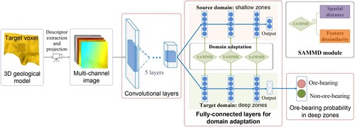
The domain adaptation network developed in this study is an extension of the convolutional neural network (CNN) for 3D MPM proposed in our previous work by Deng et al. (2022). The network takes the input of projected images of 3D geological models and learns the mineralization-associated features from the images. The network's backbone is based on the AlexNet architecture (Krizhevsky, Sutskever, and Hinton 2012), which comprises five convolutional layers and three fully-connected (FC) layers. The final fully-connected layer outputs the ore-bearing probability. Originally, the network $F_{\mathrm{\Theta }}$ with network parameters Θ is trained in a data-driven fashion by minimizing the empirical error between the output mineralization probability ${\tilde{y}}_i^{\mathrm{\prime }}=F_{\mathrm{\Theta }}\left(x_i\right)$ given the input $x_i$ and the known mineralization information $y_i$: (9) $E_{\mathrm{d}\mathrm{a}\mathrm{t}\mathrm{a}}\left(\mathrm{\Theta }\right)=-\sum _{i=1}^{m}J(F\left(x_i\right),y_i)=-\sum _{i=1}^m{y}_i\log F_{\mathrm{\Theta }}\left(x_i^s\right)$(9) where m is the number of samples with known mineralization information, and J measures the empirical error, which uses cross entropy loss in our scenario.

The minimization of Equation (9(9) $E_{\mathrm{d}\mathrm{a}\mathrm{t}\mathrm{a}}\left(\mathrm{\Theta }\right)=-\sum _{i=1}^{m}J(F\left(x_i\right),y_i)=-\sum _{i=1}^m{y}_i\log F_{\mathrm{\Theta }}\left(x_i^s\right)$(9) ) results in a CNN that fits known mineralization information and specifies 3D MPM in known areas which are generally in shallow zones. As a result of network training, the learned features, from lower to higher levels of the CNN, transit from generic to specific. In other words, the feature transferability can be substantially decreased in the FC layers on the top of CNN, which has been demonstrated by Yosinski et al. (2014). Thus, for predicting mineral prospectivity in deep zones (target domain) that have no or minimal labeling (mineralization) data, the above CNN architecture can suffer from over-fitting to shallow zones and performance degradation in deep zones. Therefore, in addition to training the network according to the labeled samples of the source domain, the SAMMD is exploited as the regularizer to improve feature transferability in FC layers.

The SAMMD measures both the feature and spatial discrepancy between source and target domains. SAMMD is minimized between FC layer features learned in shallow (source) and deep zones (target domains) to learn transferable features on FC layers of the CNN. This allows the enforcement of the distribution similarity and spatial correlation between the high-level features of CNN, thus ensuring the learned features are adaptive to the two domains. SAMMD is measured over FC layers and combined with the empirical error in the training loss (Equation 9(9) $E_{\mathrm{d}\mathrm{a}\mathrm{t}\mathrm{a}}\left(\mathrm{\Theta }\right)=-\sum _{i=1}^{m}J(F\left(x_i\right),y_i)=-\sum _{i=1}^m{y}_i\log F_{\mathrm{\Theta }}\left(x_i^s\right)$(9) ). Then, the network learning problem becomes: (10) $\begin{array}{cc}\underset{\mathrm{\Theta }}{min}\underset{\text{β},\mathrm{\Sigma }}{max}& \mathrm{Loss}(\mathrm{\Theta },\text{β},\mathrm{\Sigma })=E_{\mathrm{d}\mathrm{a}\mathrm{t}\mathrm{a}}\left(\mathrm{\Theta }\right)+\alpha {\displaystyle \sum _{l\in \mathcal{L}}{\tilde{d}}_{\mathrm{S}\mathrm{A}\mathrm{M}\mathrm{M}\mathrm{D}}(P_l,Q_l;\text{β},\mathrm{\Sigma })}\\ \mathrm{s}.\mathrm{t}.& {\displaystyle \sum _{u=1}^U{\text{β}}_u=1,{\text{β}}_u\ge 0,\mathrm{\forall }u\in 1,\dots ,U}\\ & \mathrm{\Sigma }⪰0\end{array}$(10) where $\mathcal{L}$ denotes the set of FC layers, $P_l$ and $Q_l$ are joint distribution of features and spatial postions for l-th $\mathrm{F}\mathrm{C}$ layer in source and target domains, ${\tilde{d}}_{\mathrm{S}\mathrm{A}\mathrm{M}\mathrm{M}\mathrm{D}}(P_l,Q_l;\mathrm{\Theta })$ is the empirical SAMMD estimated given the network parameters Θ and kernel parameters β and Σ, respectively, and α denotes the weighting. Note that in Equation (10(10) $\begin{array}{cc}\underset{\mathrm{\Theta }}{min}\underset{\text{β},\mathrm{\Sigma }}{max}& \mathrm{Loss}(\mathrm{\Theta },\text{β},\mathrm{\Sigma })=E_{\mathrm{d}\mathrm{a}\mathrm{t}\mathrm{a}}\left(\mathrm{\Theta }\right)+\alpha {\displaystyle \sum _{l\in \mathcal{L}}{\tilde{d}}_{\mathrm{S}\mathrm{A}\mathrm{M}\mathrm{M}\mathrm{D}}(P_l,Q_l;\text{β},\mathrm{\Sigma })}\\ \mathrm{s}.\mathrm{t}.& {\displaystyle \sum _{u=1}^U{\text{β}}_u=1,{\text{β}}_u\ge 0,\mathrm{\forall }u\in 1,\dots ,U}\\ & \mathrm{\Sigma }⪰0\end{array}$(10) ), we maximize the SAMMD loss $\sum _{l\in \mathcal{L}}{\tilde{d}}_{\mathrm{S}\mathrm{A}\mathrm{M}\mathrm{M}\mathrm{D}}(P_l,Q_l;\text{β},\mathrm{\Sigma })$ with respect to β and Σ, which optimizes the parameters β and Σ such that the two-sample test statistic is maximized. Thus, network learning is equivalent to minimizing the upper bound of the spatial-associated feature discrepancy between source and target domains. With such a training loss, the mineralization data (target labels) in Equation (10(10) $\begin{array}{cc}\underset{\mathrm{\Theta }}{min}\underset{\text{β},\mathrm{\Sigma }}{max}& \mathrm{Loss}(\mathrm{\Theta },\text{β},\mathrm{\Sigma })=E_{\mathrm{d}\mathrm{a}\mathrm{t}\mathrm{a}}\left(\mathrm{\Theta }\right)+\alpha {\displaystyle \sum _{l\in \mathcal{L}}{\tilde{d}}_{\mathrm{S}\mathrm{A}\mathrm{M}\mathrm{M}\mathrm{D}}(P_l,Q_l;\text{β},\mathrm{\Sigma })}\\ \mathrm{s}.\mathrm{t}.& {\displaystyle \sum _{u=1}^U{\text{β}}_u=1,{\text{β}}_u\ge 0,\mathrm{\forall }u\in 1,\dots ,U}\\ & \mathrm{\Sigma }⪰0\end{array}$(10) ) can be unknown. Instead, the unlabeled data and spatial coordinates in deep zones in SAMMD are leveraged to guide the network to learn transferable features from the shallow zones.

2.5. Model learning

The model learning problem in Equation (10(10) $\begin{array}{cc}\underset{\mathrm{\Theta }}{min}\underset{\text{β},\mathrm{\Sigma }}{max}& \mathrm{Loss}(\mathrm{\Theta },\text{β},\mathrm{\Sigma })=E_{\mathrm{d}\mathrm{a}\mathrm{t}\mathrm{a}}\left(\mathrm{\Theta }\right)+\alpha {\displaystyle \sum _{l\in \mathcal{L}}{\tilde{d}}_{\mathrm{S}\mathrm{A}\mathrm{M}\mathrm{M}\mathrm{D}}(P_l,Q_l;\text{β},\mathrm{\Sigma })}\\ \mathrm{s}.\mathrm{t}.& {\displaystyle \sum _{u=1}^U{\text{β}}_u=1,{\text{β}}_u\ge 0,\mathrm{\forall }u\in 1,\dots ,U}\\ & \mathrm{\Sigma }⪰0\end{array}$(10) ) is a constrained minimax optimization problem with enormous numbers of parameters. Directly using network learning algorithms such as stochastic gradient descent to learn the parameters is intractable since the optimization is constrained. Thus, we use an alternating optimization approach that iteratively updates parameters $\mathrm{\Theta },\text{β}$ and Σ to optimize the learning problem in Equation (10(10) $\begin{array}{cc}\underset{\mathrm{\Theta }}{min}\underset{\text{β},\mathrm{\Sigma }}{max}& \mathrm{Loss}(\mathrm{\Theta },\text{β},\mathrm{\Sigma })=E_{\mathrm{d}\mathrm{a}\mathrm{t}\mathrm{a}}\left(\mathrm{\Theta }\right)+\alpha {\displaystyle \sum _{l\in \mathcal{L}}{\tilde{d}}_{\mathrm{S}\mathrm{A}\mathrm{M}\mathrm{M}\mathrm{D}}(P_l,Q_l;\text{β},\mathrm{\Sigma })}\\ \mathrm{s}.\mathrm{t}.& {\displaystyle \sum _{u=1}^U{\text{β}}_u=1,{\text{β}}_u\ge 0,\mathrm{\forall }u\in 1,\dots ,U}\\ & \mathrm{\Sigma }⪰0\end{array}$(10) ). In each iteration of the algorithm, every parameter is optimized sequentially by taking the other two variables as constants.

(1)	Optimization of Θ. The network parameters are associated with the two terms in Equation (10(10) $\begin{array}{cc}\underset{\mathrm{\Theta }}{min}\underset{\text{β},\mathrm{\Sigma }}{max}& \mathrm{Loss}(\mathrm{\Theta },\text{β},\mathrm{\Sigma })=E_{\mathrm{d}\mathrm{a}\mathrm{t}\mathrm{a}}\left(\mathrm{\Theta }\right)+\alpha {\displaystyle \sum _{l\in \mathcal{L}}{\tilde{d}}_{\mathrm{S}\mathrm{A}\mathrm{M}\mathrm{M}\mathrm{D}}(P_l,Q_l;\text{β},\mathrm{\Sigma })}\\ \mathrm{s}.\mathrm{t}.& {\displaystyle \sum _{u=1}^U{\text{β}}_u=1,{\text{β}}_u\ge 0,\mathrm{\forall }u\in 1,\dots ,U}\\ & \mathrm{\Sigma }⪰0\end{array}$(10) ). It is straightforward to learn Θ in a back-propagation fashion using mini-batch stochastic gradient descent. However, in practice, the pair-wise estimate of the gradient of SAMMD can be time-consuming. Instead, the linear-time unbiased estimate of SAMMD can be adopted (Gretton, Sriperumbudur et al. 2012): (11) $\begin{array}{rll}{\hat{d}}_{\mathrm{S}\mathrm{A}\mathrm{M}\mathrm{M}\mathrm{D}}(P,Q)& =\frac{2}{m}\sum _{i=1}^{\frac{m}{2}}{h}_{\mathrm{S}\mathrm{A}\mathrm{M}\mathrm{M}\mathrm{D}}(x_{2i-1}^s,z_{2i-1}^s,x_{2i}^s,z_{2i}^s,x_{2i-1}^t,z_{2i-1}^t,x_{2i}^t,z_{2i}^t),& \\ h_{\mathrm{S}\mathrm{A}\mathrm{M}\mathrm{M}\mathrm{D}}& =k_{\varphi }(x_{2i-1}^s,x_{2i}^s)k_{\psi }(z_{2i-1}^s,z_{2i}^s)+k_{\varphi }(x_{2i-1}^t,x_{2i}^t)k_{\psi }(z_{2i-1}^t,z_{2i}^t)\\ & -k_{\varphi }(x_{2i-1}^s,x_{2i}^t)k_{\psi }(z_{2i-1}^s,z_{2i}^t)-k_{\varphi }(x_{2i}^s,x_{2i-1}^t)k_{\psi }(z_{2i}^s,z_{2i-1}^t)\end{array}$(11) We compute the gradients $\frac{\mathrm{\partial }{h}_{\mathrm{S}\mathrm{A}\mathrm{M}\mathrm{M}\mathrm{D}}}{\mathrm{\partial }{\mathrm{\Theta }}^l}$ for each tuple $v_i=$ $(x_{2i-1}^s,z_{2i-1}^s,x_{2i}^s,z_{2i}^s,x_{2i-1}^t,z_{2i-1}^t,x_{2i}^t,z_{2i}^t)$ for l-th FC-layer. Then, in each iteration, ${\mathrm{\Theta }}^l$ is updated via gradient descent according to the gradient: (12) $\frac{\mathrm{\partial }\mathrm{L}\mathrm{o}\mathrm{s}\mathrm{s}\left(\mathrm{\Theta }\right)}{\mathrm{\partial }{\mathrm{\Theta }}^l}=-\frac{\mathrm{\partial }J\left(v_i\right)}{\mathrm{\partial }{\mathrm{\Theta }}^l}+\frac{2\lambda }{m}\sum _{i=1}^{m/2}\frac{\mathrm{\partial }{h}_{\mathrm{S}\mathrm{A}\mathrm{M}\mathrm{M}\mathrm{D}}\left(v_i\right)}{\mathrm{\partial }{\mathrm{\Theta }}^l}$(12)
(2)	Optimization of β. When fixing Θ and Σ, we follow the idea of Gretton, Sriperumbudur et al. (2012) to find β that maximizes SAMMD loss in Equation (7(7) $\begin{array}{rll}{\tilde{d}}_{\mathrm{S}\mathrm{A}\mathrm{M}\mathrm{M}\mathrm{D}}(P,Q)& ={\Vert \frac{1}{m}\sum _{i=1}^m\varphi \left(x_i^s\right)\otimes \psi \left(z_i^s\right)-\frac{1}{n}\sum _{j=1}^n\varphi \left(x_j^t\right)\otimes \psi \left(z_j^t\right)\Vert }_{{\mathcal{H}}_k}^2& \\ & =\frac{1}{m^2}\sum _{i=1}^m\sum _{j=1}^m{k}_{\varphi }(x_i^s,x_j^s)k_{\psi }(z_i^s,z_j^s)+\frac{1}{n^2}\sum _{i=1}^n\sum _{j=1}^n{k}_{\varphi }(x_i^t,x_j^t)k_{\psi }(z_i^t,z_j^t)\\ & -\frac{2}{mn}\sum _{i=1}^m\sum _{j=1}^n{k}_{\varphi }(x_i^s,x_j^t)k_{\psi }(z_i^s,z_j^t).\end{array}$(7) ). To maximize the two-sample test statistic, optimization of β is equivalent to maximizing the population variance of SAMMD. Let $h_{\text{β}}$ denote a vector in which each entry is the component in terms of u-th kernel function $k_{\varphi u}$ for representing the kernel $k(x,x^{\mathrm{\prime }})$ in Equation (4(4) $k_{\varphi }(x,x^{\mathrm{\prime }})=\sum _{u=1}^U{\text{β}}_u{k}_{{}_{\varphi }u},\sum _{u=1}^U{\text{β}}_u=1,{\text{β}}_u\ge 0,$(4) ): $k_{\varphi u}(x_{2i-1}^s,x_{2i}^s)k_{\psi }(z_{2i-1}^s,z_{2i}^s)+k_{\varphi u}(x_{2i-1}^t,x_{2i}^t)k_{\psi }(z_{2i-1}^t,z_{2i}^t)-$ $k_{\varphi u}(x_{2i-1}^s,x_{2i}^t)k_{\psi }(z_{2i-1}^s,z_{2i}^t)-k_{\varphi u}(x_{2i}^s,x_{2i-1}^t)k_{\psi }(z_{2i}^s,z_{2i-1}^t)$. The variance of SAMMD can be expanded in terms of kernel parameters β as (13) $\begin{array}{rll}{\sigma }_k^2\left({\text{β}}^{\mathrm{T}}{h}_{\text{β}}\right)& =E{({\text{β}}^{\mathrm{T}}{h}_{\text{β}}-E\left({\text{β}}^{\mathrm{T}}{h}_{\text{β}}\right))}^2& \\ & ={\text{β}}^{\mathrm{T}}\mathrm{cov}\left(h_{\text{β}}\right)\text{β},\end{array}$(13) where $\mathrm{cov}\left(h_{\text{β}}\right)\in {\mathbb{R}}^{U\times U}$ is the covariance matrix of $h_{\text{β}}$. Thus, optimization of β reduces to the solution of quadratic programming (QP) problem, namely (14) $\underset{{\text{β}}^{\mathrm{T}}\zeta =1,\text{β}\ge 0}{min}{\text{β}}^{\mathrm{T}}\mathrm{cov}\left(h_{\text{β}}\right)\text{β}.$(14) The QP problem can be efficiently solved by methods such as active set, which is endowed with polynomial complexity.
(3)	Optimization of Σ. When fixing Θ and β, optimization of Σ is equivalent to maximization of the SAMMD. For simplicity, ${\hat{d}}_{\mathrm{S}\mathrm{A}\mathrm{M}\mathrm{M}\mathrm{D}}\left(\mathrm{\Sigma }\right)$ can be rewritten as: (15) $\begin{array}{rll}{\hat{d}}_{\mathrm{S}\mathrm{A}\mathrm{M}\mathrm{M}\mathrm{D}}\left(\mathrm{\Sigma }\right)& =\sum _{i=1}^{m+n}{k}_{\varphi }(x_i,x_i)& \\ & +2\sum _{i\ne j}\mathrm{s}\mathrm{i}\mathrm{g}\mathrm{n}(i,j)k_{\varphi }(x_i,x_j)\exp (-{(z_i-z_j)}^{\mathrm{T}}{\mathrm{\Sigma }}^{-1}(z_i-z_j))\end{array}$(15) where $\mathrm{s}\mathrm{i}\mathrm{g}\mathrm{n}(i,j)$ indicates the sign, which satisfies $\mathrm{sign}(i,j)=1$ if samples i and j are from the same domain and $\mathrm{sign}(i,j)=-1$ otherwise. Simply maximizing ${\hat{d}}_{\mathrm{S}\mathrm{A}\mathrm{M}\mathrm{M}\mathrm{D}}$ often leads to a trivial solution of $\mathrm{\Sigma }\to \mathrm{\infty }$. Thus, values of σ are penalized from becoming too large. Knowing that Σ is a semi-positive definite matrix, the trace of Σ is penalized instead. Therefore, σ is optimized by solving the problem: (16) $\begin{array}{cc}\underset{\mathrm{\Sigma }}{max}& {\displaystyle \sum _{i\ne j}\mathrm{s}\mathrm{i}\mathrm{g}\mathrm{n}(i,j)k_{\varphi }(x_i,x_j)\exp (-{(z_i-z_j)}^{\mathrm{T}}{\mathrm{\Sigma }}^{-1}(z_i-z_j))-\alpha \mathrm{tr}\left(\mathrm{\Sigma }\right)}\\ \mathrm{s}.\mathrm{t}.& \mathrm{\Sigma }⪰0.\end{array}$(16) where $\mathrm{tr}\left(\cdot \right)$ is the trace of Σ and α is the weight. The derivative of the objective function in Equation (16(16) $\begin{array}{cc}\underset{\mathrm{\Sigma }}{max}& {\displaystyle \sum _{i\ne j}\mathrm{s}\mathrm{i}\mathrm{g}\mathrm{n}(i,j)k_{\varphi }(x_i,x_j)\exp (-{(z_i-z_j)}^{\mathrm{T}}{\mathrm{\Sigma }}^{-1}(z_i-z_j))-\alpha \mathrm{tr}\left(\mathrm{\Sigma }\right)}\\ \mathrm{s}.\mathrm{t}.& \mathrm{\Sigma }⪰0.\end{array}$(16) ) is then: (17) $\frac{\mathrm{\partial }{\hat{d}}_{\mathrm{S}\mathrm{A}\mathrm{M}\mathrm{M}\mathrm{D}}}{\mathrm{\partial }\mathrm{\Sigma }}=\sum _{i\ne j}{\omega }_{ij}\left(\mathrm{\Sigma }\right){\mathrm{\Sigma }}^{-1}(z_i-z_j)(z_i-z_j{)}^{\mathrm{T}}{\mathrm{\Sigma }}^{-1}-\alpha \mathrm{I}=0.$(17) where ${\omega }_{ij}\left(\mathrm{\Sigma }\right)=\mathrm{s}\mathrm{i}\mathrm{g}\mathrm{n}(i,j)k_{\varphi }(x_i,x_j)\exp (-(z_i-z_j{)}^{\mathrm{T}}{\mathrm{\Sigma }}^{-1}(z_i-z_j))$. Knowing that the derivative of Σ is highly nonlinear, we linearize it by fixing Σ in ${\omega }_{ij}$ Equation (17(17) $\frac{\mathrm{\partial }{\hat{d}}_{\mathrm{S}\mathrm{A}\mathrm{M}\mathrm{M}\mathrm{D}}}{\mathrm{\partial }\mathrm{\Sigma }}=\sum _{i\ne j}{\omega }_{ij}\left(\mathrm{\Sigma }\right){\mathrm{\Sigma }}^{-1}(z_i-z_j)(z_i-z_j{)}^{\mathrm{T}}{\mathrm{\Sigma }}^{-1}-\alpha \mathrm{I}=0.$(17) ) and this implies an update for optimizing Σ, (18) ${\mathrm{\Sigma }}^{\left(t\right)}={\left(\frac{1}{\alpha }\sum _{i\ne j}{\omega }_{ij}\right({\mathrm{\Sigma }}^{(t-1)}\left)\right(z_i-z_j\left)\right(z_i-z_j{)}^{\mathrm{T}})}^{\frac{1}{2}}$(18) Here, ${\mathrm{\Sigma }}^{\left(t\right)}$ is the updated Σ in iteration step t. During implementation, the initial value of Σ is set to the identity matrix $I_{3\times 3}$, and then Σ is updated iteratively by using Equation (18(18) ${\mathrm{\Sigma }}^{\left(t\right)}={\left(\frac{1}{\alpha }\sum _{i\ne j}{\omega }_{ij}\right({\mathrm{\Sigma }}^{(t-1)}\left)\right(z_i-z_j\left)\right(z_i-z_j{)}^{\mathrm{T}})}^{\frac{1}{2}}$(18) ) until convergence.

Algorithm 1 Framework of domain alg:Framwork adaptation with SAMMD.

Input: The feature representations and space position for source and target domain observation data, $(X^s,Z^s)$ and $(X^t,Z^t)$; the label for source domain observation data, $Y^s$; learning rate η; penalty parameter λ;

Output: Network parameters Θ, multi-kernel coefficients β and matrix Σ.

1. Initialize ${\mathrm{\Theta }}^{\left(0\right)}$ randomly, ${\text{β}}^{\left(0\right)}=\frac{1}{U}{\mathbf{1}}^{\mathrm{T}}$ and ${\mathrm{\Sigma }}^{\left(0\right)}={\mathbf{I}}_{3\times 3}$, where $\mathbf{1}$ is an all-ones vector and ${\mathbf{I}}_{3\times 3}$ is an identity matrix;

2. for $epoch\tau =1\to E$ do

3.  Update Θ according to the gradient $\frac{\mathrm{\partial }\mathrm{L}\mathrm{o}\mathrm{s}\mathrm{s}(\mathrm{\Theta },\text{β},\mathrm{\Sigma })}{\mathrm{\partial }{\mathrm{\Theta }}^l}$ in Eq.(12(12) $\frac{\mathrm{\partial }\mathrm{L}\mathrm{o}\mathrm{s}\mathrm{s}\left(\mathrm{\Theta }\right)}{\mathrm{\partial }{\mathrm{\Theta }}^l}=-\frac{\mathrm{\partial }J\left(v_i\right)}{\mathrm{\partial }{\mathrm{\Theta }}^l}+\frac{2\lambda }{m}\sum _{i=1}^{m/2}\frac{\mathrm{\partial }{h}_{\mathrm{S}\mathrm{A}\mathrm{M}\mathrm{M}\mathrm{D}}\left(v_i\right)}{\mathrm{\partial }{\mathrm{\Theta }}^l}$(12) ): ${\mathrm{\Theta }}^{\left(\tau \right)}\leftarrow {\mathrm{\Theta }}^{(\tau -1)}-\eta \frac{\mathrm{\partial }\mathrm{L}\mathrm{o}\mathrm{s}\mathrm{s}({\mathrm{\Theta }}^{(\tau -1)},{\text{β}}^{(\tau -1)},{\mathrm{\Sigma }}^{(\tau -1)})}{\mathrm{\partial }\mathrm{\Theta }};$

4.  Optimize β by solving the QP problem in Equation (14(14) $\underset{{\text{β}}^{\mathrm{T}}\zeta =1,\text{β}\ge 0}{min}{\text{β}}^{\mathrm{T}}\mathrm{cov}\left(h_{\text{β}}\right)\text{β}.$(14) ): ${\text{β}}^{\left(\tau \right)}=\underset{{\text{β}}^{\mathrm{T}}\zeta =1,\text{β}\ge 0}{\arg min}{\text{β}}^{\mathrm{T}}\mathrm{cov}(h_{\text{β}}({\mathrm{\Theta }}^{\left(\tau \right)},{\mathrm{\Sigma }}^{(\tau -1)}))\text{β}$

5.  $t=0;$ ${\mathrm{\Sigma }}^{\left(t\right)}={\mathrm{\Sigma }}^{(\tau -1)}$;

6.  while not converged do

7.   Update Σ according to Equation (18(18) ${\mathrm{\Sigma }}^{\left(t\right)}={\left(\frac{1}{\alpha }\sum _{i\ne j}{\omega }_{ij}\right({\mathrm{\Sigma }}^{(t-1)}\left)\right(z_i-z_j\left)\right(z_i-z_j{)}^{\mathrm{T}})}^{\frac{1}{2}}$(18) ): ${\mathrm{\Sigma }}^{\left(t\right)}={\left(\frac{1}{\alpha }\sum _{i\ne j}{\omega }_{ij}\right({\mathrm{\Sigma }}^{(t-1)};{\mathrm{\Theta }}^{\left(\tau \right)},{\text{β}}^{\left(\tau \right)}\left)\right(z_i-z_j\left)\right(z_i-z_j{)}^{\mathrm{T}})}^{\frac{1}{2}}$

8.   t = t + 1;

9.  end while

10.  ${\mathrm{\Sigma }}^{\left(\tau \right)}={\mathrm{\Sigma }}^{\left(t\right)}$;

11.  end for

A complete procedure for our method is summarized in Algorithm 1. The effectiveness of the algorithm is validated by a case study, which will be discussed in the next section.

3. Study area and data

3.1. Study area

A case study in the Sanshandao gold deposit, eastern China (Figure 2), is undertaken to validate the effectiveness of the proposed method for 3D MPM. The Sanshandao gold deposit was chosen for two reasons. Firstly, the deposit is endowed with a ‘ladder-like’ mineralization pattern with depth (Song et al. 2015). There is a consensus that the metallogenetic mechanism between shallow and deep zones of the deposit is related but different (Bahiru and Woldai 2016; Eldursi et al. 2009; So et al. 1998; Yang et al. 2006). Secondly, the Sanshandao deposit has been explored and mined for four decades, with recent exploration progress exceeding depths of $-3,000$ m. Thus, a large amount of legacy exploration data are available as the training/validation data.

Figure 2. Geological map of the Sanshandao gold deposit (adapted from Song et al. 2021).

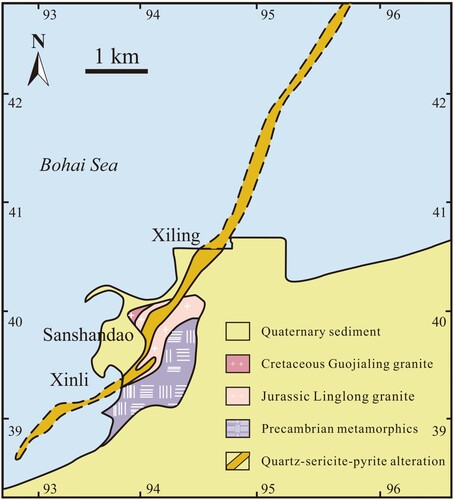
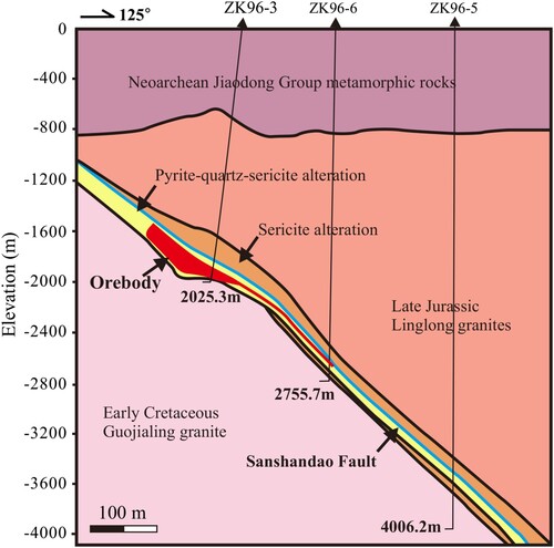
The Sanshandao gold deposit is located in the northwest of the Jiabei Uplift, 25 km north of Laizhou city. The orebodies in the Sanshandao gold deposit are located in the footwall of the Sanshandao fault. There is a consensus that the orebodies are closely related to the geometry of the Sanshandao fault (Song et al. 2021; Yan et al. 2018). The main orebodies extend approximately 1,000 m along the strike of the Sanshandao fault, with a dip angle of approximately ${40}^{\circ }$ and an extended depth of about 1,500 m. In recent years, many deep drill holes in the deposit revealed the alteration and mineralization at −1170 to −3555 m (Figure 3). By including the newly discovered gold resources on the seabed in the north of the mining area, the total resource reserves of the orebodies are as high as 600 t (Song et al. 2015), making it one of the largest gold deposits in China.

Figure 3. Mineralization-alteration zoning pattern (at section line # 96) of the Sanshandao gold deposit (adapted from Hu et al. 2013).

3.2. Data preparation

The current and legacy exploration datasets for the deposit were retrieved to predict mineral prospectivity for the Sanshandao deposit. The data collected contains 27 cross-sections, 121 drillholes, and 48,119 gold assays (until June 2019). Here, the interval of the parallel cross-sections is generally 100 m. The geological profiles at each cross-section are generated according to drill holes and controlled source audio-frequency magnetotellurics (CSAMT). The gold grades in drillhole samples were determined by fire assay, followed by flame atomic absorption analysis. The cross-section profiles, drillhole data, and the associated gold assay data were digitalized. The digitalized dataset forms the GIS database for the Sanshandao gold deposit. Based on the GIS database, the 3D models of the Sanshandao gold deposit were then reconstructed.

Since the geometry of the Sanshandao fault controls the gold mineralization, a 3D geologic model of the Sansandao fault was constructed to represent its geometry. In the 3D modeling process, 3D contours of the fault surface were delineated according to the cross-section profiles. Then, the geometry between the 3D contours was interpolated using the implicit modeling method (Macêdo, Paulo Gois, and Velho 2011), resulting in the 3D model of the Sanshandao fault (Figure 4(a)). The mesh of the 3D models were generated using the surface generation package of CGAL (Fabri and Pion 2009) with 30 m resolution for triangular faces. The 3D models of orebodies of the Sanshandao deposit (Figure 4(b)) were generated using a procedure analogous to that of the fault model. Then, the area of the Sanshandao deposit was then partitioned into regular voxels. The size of each voxel is ${25}^3{\mathrm{m}}^3$. To reflect the 3D distribution of mineralization, we interpolated gold grades using the Kriging method according to Au assay samples. The key characteristics of the data used in this study are summarized in Table 1.

Figure 4. 3D models of Sanshandao faults (a), orebodies (Au grade ≥ 1g/t) (b), and drillholes (c). Left column: down-plunge views, right column: top views.

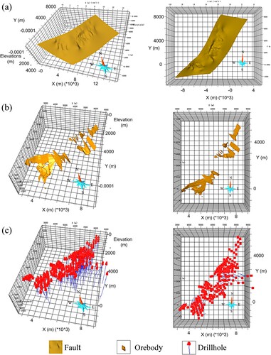
Table 1. Summary of data characteristics.

Data type	Resolution	Analytic/Construction method
Geological profile	∼100 m	Drill hole / CSAMT
Gold assay data	Sampling resolution ∼1 m at drill holes	Fire assay, followed by flame atomic absorption analysis
3D geologic model	Triangular mesh resolution ∼30 m	Implicit modeling
3D voxel model	$25\mathrm{m}\times 25\mathrm{m}\times 25\mathrm{m}$	Voxelization of 3D geologic model / Kriging interpolation

4. Results

4.1. Mineral prospectivity modeling

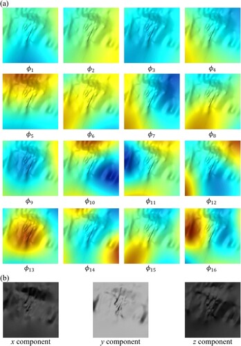
To predict the mineral prospectivity in deep-seated areas, space-associated models were built to transfer the association learned in shallow areas of the Sanshandao deposit. The workflow utilized previously by Deng et al. (2022) was used to generate multi-channel images input to the deep neural network (Figure 1). The workflow includes the computations of shape descriptors for the 3D fault model (Figure 5) and the projection of shape descriptors onto multi-channel images (Figure 6) for the voxels. Here, the multi-channel image has a resolution of $224\times 224$ and includes 20 channels, i.e. 19 channels projected from shape descriptors as described above and one extra channel representing the surface distance to the voxel. As in Deng et al. (2022), it is justified that these channels can encode the information of geological control from the geological boundary (i.e. the Sanshandao fault) to the locations of the voxels.

Figure 5. Shape descriptors of Laplace–Beltrami eigenfunctions (a) and surface normals (b) of the Sanshandao fault.

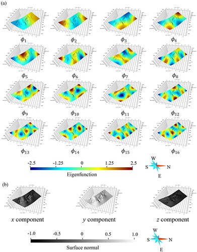
Figure 6. Projection results of the shape descriptors for target voxels: Laplace–Beltrami eigenfunctions (a) and surface normals (b).

To build the mineral prospectivity model in a domain adaptation fashion, the area of the Sanshandao deposit was partitioned into source and target domain according to the data availability of each area. The ‘known’ area corresponds to voxels inside the orebody model, and the remaining voxels are controlled by drillholes. These known area voxels, 48,119 voxels in the case study, form the source domain examples. According to the cutoff Au grade of 1.0 g/t, every source domain example was labeled as ore-bearing or non-ore-bearing, resulting in 17,822 ore-bearing voxels and 30,297 non-ore-bearing voxels. The known area voxels were partitioned into training and validation sets. 8,966 known voxels with depths between −1500 to −3000 m were used for validation. In addition, 31,358 unknown voxels in the deep zones were taken as the target domain examples in the domain adaptation.

The proposed approach was implemented using PyTorch, an open-source Python machine learning library developed by Facebook AI Research (FAIR) (Paszke et al. 2019). In this framework, the space-associated deep adaptation network was trained in an end-to-end manner. RAdam (Rectified Adam) (Liu et al. 2019) was used to calculate gradients of the joint loss function in Equation (10(10) $\begin{array}{cc}\underset{\mathrm{\Theta }}{min}\underset{\text{β},\mathrm{\Sigma }}{max}& \mathrm{Loss}(\mathrm{\Theta },\text{β},\mathrm{\Sigma })=E_{\mathrm{d}\mathrm{a}\mathrm{t}\mathrm{a}}\left(\mathrm{\Theta }\right)+\alpha {\displaystyle \sum _{l\in \mathcal{L}}{\tilde{d}}_{\mathrm{S}\mathrm{A}\mathrm{M}\mathrm{M}\mathrm{D}}(P_l,Q_l;\text{β},\mathrm{\Sigma })}\\ \mathrm{s}.\mathrm{t}.& {\displaystyle \sum _{u=1}^U{\text{β}}_u=1,{\text{β}}_u\ge 0,\mathrm{\forall }u\in 1,\dots ,U}\\ & \mathrm{\Sigma }⪰0\end{array}$(10) ), which provides a dynamic heuristic method to provide automated variance decay, thus eliminating the need for manual tuning involved in warm-up process during training. The domain adaptation prospectivity network was trained from scratch rather than pre-trained from large-scale datasets. Dropout regularization was applied to both FC6 and FC7 during training.

4.2. Performance assessment

The results were compared with several leading MPM methods and another domain adaption variant to validate the performance of the proposed method. To verify the contribution of domain adaptation, CNNs (Deng et al. 2022), random forests (Carranza and Laborte 2015b; Xiang et al. 2020) and multi-layer perceptrons (Abedi and Norouzi 2012; Ghezelbash, Maghsoudi, and Carranza 2020)were chosen for comparison. Here, the CNN is equivalent to the backbone of the spatial-associated domain adaptation network in Figure 1. The random forest and the multi-layer perceptrons are statistical learning-based methods and associate the hand-crafted predictor variables with mineralization. In random forest and multi-layer perceptrons, the predictor variables are the same as those in Mao et al. (2019).

To specifically verify the contribution of SAMMD, another mineral prospectivity model was built based on domain adaptation. The domain adaptation model is a variant of the network in Figure 1, in which the SAMMD module is replaced with the original MMD proposed by Long et al. (2015). The same setting of source and target domains was used to train the MMD model.

The five methods described above were then compared according to their receiver operating characteristic (ROC) curves (Barreno, Cardenas, and Tygar 2007) and success-rate curves (Agterberg and Bonham-Carter 2005). The ROC curve plots the actual positive rate (TPR) variations against the false positive rate (FPR) at different decision thresholds to distinguish prospective areas. The area under the curve (AUC) method was employed to assess the prediction accuracy of the compared methods. The AUC is the probability that a random positive example is estimated more highly than a random negative example. The success-rate curve plots the proportion of the prospective regions to prospective areas against the proportion of prospective areas to the whole study area at different thresholds to distinguish prospective areas. A higher success rate indicates that, given a certain percentage of perspective areas, more orebodies can be successfully targeted and thus the estimated model has a higher targeting efficiency. Only the examples in the validation set were used to plot ROC curves.

Several interesting characteristics are observed from both AUCs and success rates (Figure 7). Firstly, the deep learning models (CNN, MMD, and SAMMD) achieve solid improvement over statistical learning models that use hand-crafted predictor variables. This outcome indicates that the CNN backbone (Figure 1) can learn features more closely associated with the deep mineralization on top of the network. Deep learning approaches have the advantage of being able to learn complex and abstract features that may not be easily identified by conventional statistical methods. However, they require large-scale training data. Thereby, the transfer learning scheme is advocated to leverage data from other domains to improve the performance of deep learning models.

Figure 7. ROC curves (a) and success-rate curves (b) for the five evaluated prospectivity models. The SAMMD-based model attains the best performance among the five tested methods.

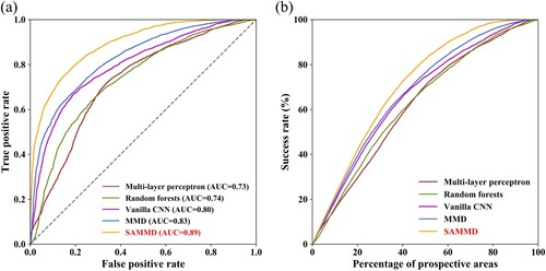
It is seen that the two deep transfer learning models (SAMMD and MMD) perform better than the vanilla CNN model. This outcome reflects the discrepancy between shallow and deep zones, demonstrating that minimizing the feature discrepancy in the mineral prospectivity model improves the transferability of features to deep mineralization. The domain adaption approaches allow us to transfer information from related domains, which considers domain discrepancy in applications while reducing the amount of data required for training. In 3D MPM, when the domain discrepancy is associated with spatial locations, simply considering the feature discrepancy across domains can be insufficient to effectively quantify domain discrepancy. Notably, the SAMMD model is substantially superior to the original MMD model. In contrast to the original MMD that measures feature transferability only from the feature space, the SAMMD further incorporates the proximity of geospace into the feature discrepancy assessment. The results of SAMMD demonstrate that leveraging the characteristics of spatial correlation and spatial variance can correct the measure of feature transferability. This suggests that minimizing SAMMD in spatial-associated domain adaptation networks can promote positive transfer while suppressing excess transfer in the transfer learning. As indicated from AUCs and success rate curves, the prospectivity model based on SAMMD can be more sensitive to deep mineralization and exclude more false positives in delineating prospective areas, reflecting that SAMMD is crucial to ensure prediction accuracy and targeting efficiency in 3D MPM. Thus, the spatial-associated domain adaptation enables us to use spatial information to guide the feature transfer and boost the performance of 3D MPM.

4.3. Interpretation of SAMMD

Theoretical analysis has shown that the risk of the target domain is bounded by the discrepancy between source and target domains (Ben-David et al. 2010; Mansour, Mohri, and Rostamizadeh 2009). To test the risk of the target domain for the three leading models (CNN, MMD and SAMMD), the domain discrepancy and the empirical risk were evaluated. Since the domain discrepancy of joint distributions over feature space and geospace cannot be measured by generic metrics like the $\mathcal{A}$-distance described by Ben-David et al. (2010), the SAMMD defined in Equation (7(7) $\begin{array}{rll}{\tilde{d}}_{\mathrm{S}\mathrm{A}\mathrm{M}\mathrm{M}\mathrm{D}}(P,Q)& ={\Vert \frac{1}{m}\sum _{i=1}^m\varphi \left(x_i^s\right)\otimes \psi \left(z_i^s\right)-\frac{1}{n}\sum _{j=1}^n\varphi \left(x_j^t\right)\otimes \psi \left(z_j^t\right)\Vert }_{{\mathcal{H}}_k}^2& \\ & =\frac{1}{m^2}\sum _{i=1}^m\sum _{j=1}^m{k}_{\varphi }(x_i^s,x_j^s)k_{\psi }(z_i^s,z_j^s)+\frac{1}{n^2}\sum _{i=1}^n\sum _{j=1}^n{k}_{\varphi }(x_i^t,x_j^t)k_{\psi }(z_i^t,z_j^t)\\ & -\frac{2}{mn}\sum _{i=1}^m\sum _{j=1}^n{k}_{\varphi }(x_i^s,x_j^t)k_{\psi }(z_i^s,z_j^t).\end{array}$(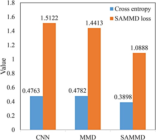7) ) was used as the cross-domain discrepancy metric. Here, the SAMMD loss was computed at the top layers of network models. On the other hand, the cross-entropy loss for the validation set was employed to measure the empirical risk of the target domain. Figure 8 illustrates the outcomes of SAMMD and cross-entropy data. According to the SAMMD, the features learned by CNN have the highest cross-domain discrepancy, followed by those learned by the MMD model, and the features learned by the SAMMD model yield the smallest metric of cross-domain discrepancy. This demonstrates that deep features learned from shallow zones by CNN cannot be simply generalized to the target domain. While the features learned by the MMD model show a smaller cross-domain discrepancy than the vanilla CNN, the MMD model, as a variant of CNN considering domain discrepancy of individual features, cannot substantially reduce the spatial-associated cross-domain discrepancy of features. In comparison, the features learned by the SAMMD model reduce the cross-domain discrepancy by minimizing the joint distribution discrepancy over features and geospace, suggesting the necessity of introducing spatial factors into transfer learning in 3D MPM. On the other hand, the cross-entropies of CNN and MMD are nearly identical, with the cross-entropy of MMD slightly higher than that of CNN. In contrast, the SAMMD model attains the minimum cross-entropy. The results of cross-entropy suggest that simply minimizing the feature discrepancy between shallow and deep zones cannot yield safely transferable features to indicate the mineral prospectivity for the deep zones (target domains) in 3D MPM. Notably, when minimizing the joint discrepancy over features and geospace, the learned features are considerably more transferable to the deep zones and the empirical risk of the target domain is essentially reduced. Therefore, spatial factors are essential to guide feature transfer from shallow to deep zones in 3D MPM.

Figure 8. Cross entropy and SAMMD loss resulting from CNN, MMD and SAMMD models.

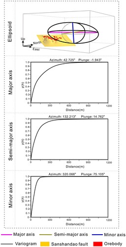
In the transfer learning process, the spatial kernel $k_{\psi }$ defined in Equation (8(8) $k_{\psi }(z_i,z_j)=\exp (-{(z_i-z_j)}^T{\mathrm{\Sigma }}^{-1}(z_i-z_j)),$(8) ) is optimized to maximize the SAMMD. In particular, the learned parameter Σ reflects spatial anisotropy of feature transferability. As shown in the Appendix 1, the anisotropy can be interpreted by estimating the singular value decomposition (SVD) of Σ. The directional variograms interpreted from Σ show evident spatial anisotropy (Figure 9). The variogram of the major axis has the most extensive range. The major axis roughly coincides with the strike directions of the Sanshandao fault and the orebodies, suggesting the domain discrepancy varies gently along the strike direction of the Sanshandao fault. Since the Sanshandao fault is the ore-controlling structure, the low domain discrepancy along the strike direction of the Sanshandao fault suggests a similar metallogenic mechanism at roughly the same depth along the Sanshandao fault. The direction of the semi-major axis is roughly consistent with the horizontal extending direction of major orebodies at Sanshandao (Song et al. 2015). The variogram range of the semi-major axis is nearly 2/3 of the range for the major axis, suggesting that the domain discrepancy varies moderately along the horizontal extending direction of orebodies. The variogram of minor axis has the smallest range, which is approximately 1/5 of the range for the major axis. This small range highlights the substantial variation of domain discrepancy along the deep direction.

Figure 9. Variograms corresponding to the SAMMDs for 3D MPM at Sanshandao.

4.4. 3D predictive mapping and target appraisal

Given the mineral probability predicted by the 3D MPM models, potential areas in the deep zones of the study area can be identified for future exploration. To determine the potential areas, an optimal threshold of probability was chosen to separate high-probability areas from the low-probability background. Following the work of (Chen and Wu 2017; Deng et al. 2022), the probability value with the maximum Youden index (MYI) (Ruopp et al. 2008; Youden 1950) was chosen as the threshold. Table 2 lists the MYIs and corresponding thresholds for the SAMMD model and the counterpart MMD model. The SAMMD model exhibits higher MYIs, consistent with the results of ROC and success rate curves. The thresholds for SAMMD and MMD are both higher than the prior probability (0.3703) of ore-bearing voxels.

Table 2. MYIs and the corresponding thresholds for the SAMMD and the MMD-based models.

Prospectivity model	MYI	Probability
$\mathrm{S}\mathrm{A}\mathrm{M}\mathrm{M}\mathrm{D}$	0.6251	0.4546
MMD	0.5197	0.4065

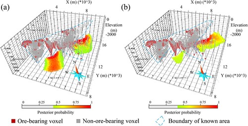
Figure 10 shows the potential mineralization areas predicted by MMD and SAMMD models. Both of them identify two potential areas: One is located in the northern segment of the study area, and the other one is located in the middle segment of the study area. In the northern segment, the potential areas identified by the two methods overlap to a large extent. Both of the potential areas are plate-shaped and are likely the NE extension of the orebodies. In the middle segment, the SAMMD and MMD methods both identify a potential area extending from the main orebodies. However, the SAMMD method predicts higher gold prospectivity over a larger potential area in the segment compared to the MMD method. Considering that this shallow zone above this potential area hosts a large amount of gold mineralization and orebodies have been discovered in other deep zones in the study area, we argue that the high potential area predicted by SAMMD could be the deep extension of shallow orebodies and has a reasonable potential for future exploration.

Figure 10. The high-potential areas resulting from the SAMMD (a) and the MMD (b) models.

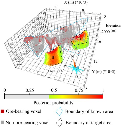
Overall, two potential areas are delineated by the SAMMD model (Figure 11). Target I extends from the northern segment of orebodies in the northwest direction and is located at elevations from −1600 to −2200 m. Target II is sited at elevations from −1000 to −2000 m beneath the middle segment of the orebodies, which is considered to be their deep extension.

Figure 11. Two mineral exploration targets identified by the SAMMD model.

5. Discussion and conclusions

In this paper, we have proposed a spatial-associated domain adaptation method for 3D MPM. Unlike existing methods for 3D MPM, this evolving technique has several distinct advantages. Firstly, the proposed method considers the differences in metallogenic mechanism between the shallow known zones and deep unknown zones. This is achieved by introducing a transfer learning paradigm to 3D MPM and casting the 3D MPM as a domain adaptation problem. This approach allows us to avoid the bias inherent in the mineral prospectivity model constructed solely based on examples from shallow known zones. As a result, it provides a more adaptive model that can effectively prospect deep unknown zones. Secondly and more importantly, the proposed method can bridge the domain discrepancy concerning not only the features but the geospace, which is a major contributing factor to the differences in metallogenic mechanism. This ensures the measure of spatial-associated domain discrepancy in 3D MPM. The resulting workflow prevents the limitation of MPM that solely relies on across-domain features or predictor variables to predict mineral prospectivity. Finally, the proposed method combines the scheme of spatial-associated domain adaptation with a deep learning framework. The model leads to a spatial-associated deep adaption network that learns feature representation ‘end-to-end’. The learned features are indicative of mineralization and are transferable across the geospace for 3D MPM. As demonstrated in a case study of deep mineral prospectivity modeling, the advantages of the proposed method enable a substantial improvement in the prediction accuracy and targeting efficiency in 3D MPM, providing a novel and effective tool for deep exploration targeting.

While the proposed method addresses the mineral prospectivity modeling problem (i.e. solving the ‘where’ problem) by assessing the difference of metallogenic mechanism between shallow and deep zones, how to extend the proposed method to achieve quantitative mineral resource estimation (i.e. solving the ‘how much’ problem) by considering the domain discrepancy between shallow and deep zones is a promising avenue for our future work. To estimate the ore-bearing ratio in deep zones, in particular, we will scale SAMMD and the associated spatial-associated domain adaptation network to the regression task for the prediction of the ore-bearing ratio in deep zones. We anticipate that this will further improve the applicability and reliability of GIS in mineral exploration targeting.

Data and codes availability statement

The codes that support the findings of this study are available with the identifier at the private link (https://figshare.com/s/1b1de1850615d1c98154).

The data for this study is confidential geological data and written consent was not given for it to be shared publicly, so due to the sensitive nature of the research supporting data is not available.

Acknowledgments

We thank the anonymous reviewers for their constructive suggestions to help us improve the manuscript of this paper.

Disclosure statement

No potential conflict of interest was reported by the author(s).

Additional information

Funding

This research was funded by the National Natural Science Foundation of China (Nos. 41972309, 42272344, 42030809, 42072325, 72088101) and National Key R&D Program of China (No. 2019YFC1805905).

Appendices

Appendix 1.

Relation between the spatial kernel $k_{\psi }(z_i,z_j)$ and the variogram of Gaussian model in 3D space

The Gaussian model representing the geometric anisotropy in 3D space has the form (Allard, Senoussi, and Porcu 2016; Chiles and Delfiner 2009): ({A1) $\gamma \left(h\right)=1-\exp (-\Vert Ah{\Vert }^2),$({A1) where h is the lag and A is the product of a diagonal matrix D and a rotation matrix $R:A=$ DR. Here, the row vectors of R correspond to the main directions of anisotropy and the diagonal entries $b_i$ of A are equal to $1/a_i$, where $a_i$ is the range in i-th main direction of anisotropy.

Given the spatial kernel ({A2) $k_{\psi }(z_i,z_j)=\exp (-{(z_i-z_j)}^T{\mathrm{\Sigma }}^{-1}(z_i-z_j))$({A2) we can use singular value decomposition (SVD) to decompose the matrix ${\mathrm{\Sigma }}^{-1}$. Since Σ can be regarded as the covariance matrix, which is a real symmetric matrix, the SVD of ${\mathrm{\Sigma }}^{-1}$ has the form: ({A3) ${\mathrm{\Sigma }}^{-1}=V{\mathrm{\Lambda }}^{-1}{V}^{\mathrm{T}}$({A3) where V is an orthogonal matrix in which each vector is an eigenvector of Σ and Λ is a diagonal matrix in which each diagonal entry is an eigenvalue of Σ.

Inserting Equation (A3({A3) ${\mathrm{\Sigma }}^{-1}=V{\mathrm{\Lambda }}^{-1}{V}^{\mathrm{T}}$({A3) ) into Equation (A2({A2) $k_{\psi }(z_i,z_j)=\exp (-{(z_i-z_j)}^T{\mathrm{\Sigma }}^{-1}(z_i-z_j))$({A2) ), we have ({A4) $\begin{array}{rll}{k}_{\psi }(z_i,z_j)& =\exp (-{(z_i-z_j)}^{T}V{\mathrm{\Lambda }}^{-1}{V}^T(z_i-z_j))& \\ & =\exp (-{(z_i-z_j)}^{T}V{\mathrm{\Lambda }}^{-\frac{1}{2}}{\mathrm{\Lambda }}^{-\frac{1}{2}}{V}^T(z_i-z_j))\\ & =\exp (-{\Vert {\mathrm{\Lambda }}^{-\frac{1}{2}}{V}^T(z_i-z_j)\Vert }^2)\\ & =\exp (-\Vert \tilde{A}h{\Vert }^2),\end{array}$({A4) where $\tilde{A}={\mathrm{\Lambda }}^{-\frac{1}{2}}{V}^T$ and $h=z_i-z_j$. Note that $\tilde{A}=={\mathrm{\Lambda }}^{-\frac{1}{2}}{V}^T$ indicates the matrix $\tilde{A}$, like the A in Equation (A1({A1) $\gamma \left(h\right)=1-\exp (-\Vert Ah{\Vert }^2),$({A1) ), is the product of a diagonal matrix and rotation (orthogonal) matrix.

Under the the assumption of second-order stationarity, the variogram is related to the covariance, formulated as: ({A5) $\gamma \left(h\right)=\mathrm{cov}\left(0\right)-\mathrm{cov}\left(h\right),$({A5) Combining Equations (A1({A1) $\gamma \left(h\right)=1-\exp (-\Vert Ah{\Vert }^2),$({A1) ), (A4({A4) $\begin{array}{rll}{k}_{\psi }(z_i,z_j)& =\exp (-{(z_i-z_j)}^{T}V{\mathrm{\Lambda }}^{-1}{V}^T(z_i-z_j))& \\ & =\exp (-{(z_i-z_j)}^{T}V{\mathrm{\Lambda }}^{-\frac{1}{2}}{\mathrm{\Lambda }}^{-\frac{1}{2}}{V}^T(z_i-z_j))\\ & =\exp (-{\Vert {\mathrm{\Lambda }}^{-\frac{1}{2}}{V}^T(z_i-z_j)\Vert }^2)\\ & =\exp (-\Vert \tilde{A}h{\Vert }^2),\end{array}$({A4) ), and (A5({A5) $\gamma \left(h\right)=\mathrm{cov}\left(0\right)-\mathrm{cov}\left(h\right),$({A5) ), the spatial kernel function $k_{\psi }(z_i,z_j)$ can be regarded as the covariance function associated with the variogram of Gaussian model $\gamma \left(h\right)$. In other words, the relation between $k_{\psi }(z_i,z_j)$ and $\gamma \left(h\right)$ is formulated as: ({A6) $\begin{array}{rll}\gamma \left(h\right)& =1-\exp (-\Vert \tilde{A}h{\Vert }^2).& \\ & =1-\exp (-{(z_i-z_j)}^T{\mathrm{\Sigma }}^{-1}(z_i-z_j))\\ & =1-k_{\psi }(z_i,z_j).\end{array}$({A6) Therefore, the spatial kernel $k_{\psi }(z_i,z_j)$ and the variogram of Gaussian model for representing geometric anisotropy in 3D space is equivalent.

According to relation between $k_{\psi }(z_i,z_j)$ and $\gamma \left(h\right)$, $k_{\psi }(z_i,z_j)$ can be used to interpret feature transferability in 3D space. The eigenvectors of Σ indicate the main directions of anisotropy, i.e. the directions with maximized/minimized/tertiary feature transferability, and the singular values of Σ indicate the range of variation in three main directions.

Appendix 2.

The entry of matrix Σ in definition of spatial kernel $k_{\psi }(z_i,z_j)$

The spatial kernel $k_{\psi }(z_i,z_j)$ can be written as ({A7) $k_{\psi }(z_i,z_j)=\exp (-h^T{\mathrm{\Sigma }}^{-1}h),$({A7) where $h=z_i-z_j$ is the 3D vector representing the spatial separation between $z_i$ and $z_j$

Let ${\sigma }_{kl},k,l=1,2,3,$ denotes the entry of matrix Σ in Equation (A7({A7) $k_{\psi }(z_i,z_j)=\exp (-h^T{\mathrm{\Sigma }}^{-1}h),$({A7) ). Expanding Equation (A7({A7) $k_{\psi }(z_i,z_j)=\exp (-h^T{\mathrm{\Sigma }}^{-1}h),$({A7) ) yields, (A8) $\begin{array}{rll}{k}_{\psi }(z_i,z_j)& =\exp (-\sum _{k=1}^3\sum _{l=1}^3{\sigma }_{kl}{h}_k{h}_l)& \\ & =\exp (-\sum _{k=1}^3{\sigma }_{kk}{h}_k^2-2\sum _{k\ne l}{\sigma }_{kl}{h}_k{h}_l),\end{array}$(A8) where the subscript of h, say, $h_k$, is the k-th component of h.

We show that $k_{\psi }(z_i,z_j)$ is consistent with the variogram $\gamma \left(h\right)$ that represents geometric anisotropy in 3D space (Appendix 1). To represent geometric anisotropy the variogram $\gamma \left(h\right)$ can be estimated in a new orthogonal coordinate system as: $\gamma \left(h\right)={\gamma }_0\left(\sum _{k=1}^3{b}_k{h}_k^{\prime }\right)$ (Chiles and Delfiner 2009), where $h_k^{\prime }$ is the k-th component of the spatial separation measured in the new orthogonal coordinate system. According to Equation (A5({A5) $\gamma \left(h\right)=\mathrm{cov}\left(0\right)-\mathrm{cov}\left(h\right),$({A5) ), we have ({A9) $k_{\psi }(z_i,z_j)=\exp (-\sum _{k=1}^3{b}_k^2{h_k^{\prime }}^2).$({A9) This implies the off-diagonal entry ${\sigma }_{kl},k\ne l$ in Equation (A8(A8) $\begin{array}{rll}{k}_{\psi }(z_i,z_j)& =\exp (-\sum _{k=1}^3\sum _{l=1}^3{\sigma }_{kl}{h}_k{h}_l)& \\ & =\exp (-\sum _{k=1}^3{\sigma }_{kk}{h}_k^2-2\sum _{k\ne l}{\sigma }_{kl}{h}_k{h}_l),\end{array}$(A8) ) is zero if the new orthogonal coordinate system coincide to the original coordinate system. Otherwise, it invokes rotations to the original coordinate in order to form the new coordinate system that satisfies Equation (A9({A9) $k_{\psi }(z_i,z_j)=\exp (-\sum _{k=1}^3{b}_k^2{h_k^{\prime }}^2).$({A9) ) (Chiles and Delfiner 2009). Such rotations will lead to the correlation of original spatial dimensions in the new coordinate system. Thus, the off-diagonal ${\sigma }_{kl}$ entry measures the correlation between the k-dimension and l-dimension in 3D space.

References

- Abedi, Maysam, and Gholam-Hossain Norouzi. 2012. “Integration of Various Geophysical Data with Geological and Geochemical Data to Determine Additional Drilling for Copper Exploration.” Journal of Applied Geophysics 83:35–45. https://doi.org/10.1016/j.jappgeo.2012.05.003.
- Agterberg, Frederik P., and Graeme F. Bonham-Carter. 2005. “Measuring the Performance of Mineral-potential Maps.” Natural Resources Research 14 (1): 1–17. https://doi.org/10.1007/s11053-005-4674-0.
- Allard, Denis, Rachid Senoussi, and Emilio Porcu. 2016. “Anisotropy Models for Spatial Data.” Mathematical Geosciences 48 (3): 305–328. https://doi.org/10.1007/s11004-015-9594-x.
- Bahiru, Engdawork Admassu, and Tsehaie Woldai. 2016. “Integrated Geological Mapping Approach and Gold Mineralization in Buhweju Area, Uganda.” Ore Geology Reviews 72:777–793. https://doi.org/10.1016/j.oregeorev.2015.09.010.
- Barreno, Marco, Alvaro Cardenas, and J. Doug Tygar. 2007. “Optimal ROC Curve for A Combination of Classifiers,.Advances in Neural Information Processing Systems.Vancouver, B.C., Canada.
- Ben-David, Shai, John Blitzer, Koby Crammer, Alex Kulesza, Fernando Pereira, and Jennifer Wortman Vaughan. 2010. “A Theory of Learning From Different Domains.” Machine Learning 79 (1-2): 151–175. https://doi.org/10.1007/s10994-009-5152-4.
- Bonham-Carter, Graeme F. 1994. “Geographic Information Systems for Geoscientists-modeling with GIS.” Computer Methods in the Geoscientists 13:398. https://doi.org/10.1016/0098-3004(95)90019-5.
- Bousmalis, Konstantinos, George Trigeorgis, Nathan Silberman, Dilip Krishnan, and Dumitru Erhan. 2016. “Domain Separation Networks.” CoRR. http://arxiv.org/abs/1608.06019.
- Brown, Warick M., T. D. Gedeon, D. I. Groves, and R. G. Barnes. 2000. “Artificial Neural Networks: a New Method for Mineral Prospectivity Mapping.” Australian Journal of Earth Sciences 47 (4): 757–770. https://doi.org/10.1046/j.1440-0952.2000.00807.x.
- Carranza, Emmanuel John M. 2008. Geochemical Anomaly and Mineral Prospectivity Mapping in GIS. Amsterdam: Elsevier.
- Carranza, Emmanuel John M., and Alice G. Laborte. 2015a. “Data-driven Predictive Mapping of Gold Prospectivity, Baguio District, Philippines: Application of Random Forests Algorithm.” Ore Geology Reviews 71:777–787. https://doi.org/10.1016/j.oregeorev.2014.08.010.
- Carranza, Emmanuel John M., and Alice G. Laborte. 2015b. “Random Forest Predictive Modeling of Mineral Prospectivity with Small Number of Prospects and Data with Missing Values in Abra (Philippines).” Computers & Geosciences 74:60–70. https://doi.org/10.1016/j.cageo.2014.10.004.
- Chen, Yongliang. 2015. “Mineral Potential Mapping with a Restricted Boltzmann Machine.” Ore Geology Reviews 71:749–760. https://doi.org/10.1016/j.oregeorev.2014.08.012.
- Chen, Yongliang, and Wei Wu. 2017. “Mapping Mineral Prospectivity Using An Extreme Learning Machine Regression.” Ore Geology Reviews 80:200–213. https://doi.org/10.1016/j.oregeorev.2016.06.033.
- Chiles, Jean-Paul, and Pierre Delfiner. 2009. Geostatistics: Modeling Spatial Uncertainty. Vol. 497. John Wiley & Sons.
- Cloetingh, S., and Y. Y. Podladchikov. 2000. “Perspectives on Tectonic Modeling.” Tectonophysics 320 (3-4): 169–173. https://doi.org/10.1016/S0040-1951(00)00154-2.
- Deng, Hao, Yang Zheng, Jin Chen, Shuyan Yu, Keyan Xiao, and Xiancheng Mao. 2022. “Learning 3D Mineral Prospectivity From 3D Geological Models Using Convolutional Neural Networks: Application to a Structure-controlled Hydrothermal Gold Deposit.” Computers & Geosciences 161:105074. https://doi.org/10.1016/j.cageo.2022.105074.
- Ding, Zhengming, and Yun Fu. 2017. “Robust Transfer Metric Learning for Image Classification.” IEEE Transactions on Image Processing 26:660–670. https://doi.org/10.1109/TIP.2016.2631887.
- Eldursi, Khalifa, Yannick Branquet, Laurent Guillou-Frottier, and Eric Marcoux. 2009. “Numerical Investigation of Transient Hydrothermal Processes Around Intrusions: Heat-transfer and Fluid-circulation Controlled Mineralization Patterns.” Earth and Planetary Science Letters 288 (1-2): 70–83. https://doi.org/10.1016/j.epsl.2009.09.009.
- Fabri, Andreas, and Sylvain Pion. 2009. “CGAL: The Computational Geometry Algorithms Library.In Proceedings of the 17th ACM SIGSPATIAL International Conference on Advances in Geographic Information Systems.Beijing, China.
- Fallara, Francine, Marc I. Legault, and Rabeau Olivier. 2006. “3-D Integrated Geological Modeling in the Abitibi Subprovince (Québec, Canada): Techniques and Applications.” Exploration and Mining Geology 15 (1-2): 27–43. https://doi.org/10.2113/gsemg.15.1-2.27.
- Ghezelbash, Reza, Abbas Maghsoudi, and Emmanuel John M. Carranza. 2020. “Sensitivity Analysis of Prospectivity Modeling to Evidence Maps: Enhancing Success of Targeting for Epithermal Gold, Takab District, NW Iran.” Ore Geology Reviews 120:103394. https://doi.org/10.1016/j.oregeorev.2020.103394.
- Gong, Boqing, Kristen Grauman, and Fei Sha. 2013. “Connecting the Dots with Landmarks: Discriminatively Learning Domain-Invariant Features for Unsupervised Domain Adaptation.” In Proceedings of the 30th International Conference on Machine Learning, edited by Sanjoy Dasgupta and David McAllester, Vol. 28 of Proceedings of Machine Learning Research, Atlanta, Georgia, USA, 17–19 Jun, 222–230. PMLR.
- Goodchild, Michael F. 2003. “The Fundamental Laws of GIScience.” http://csiss.ncgia.ucsb.edu/aboutus/presentations/files/goodchild_ucgis_jun03.pdf.
- Gretton, Arthur, Karsten M. Borgwardt, Malte J. Rasch, Bernhard Schölkopf, and Alexander Smola. 2012. “A Kernel Two-sample Test.” Journal of Machine Learning Research 13:723–773. https://doi.org/10.1142/S0219622012400135.
- Gretton, Arthur, Bharath Sriperumbudur, Dino Sejdinovic, Heiko Strathmann, Sivaraman Balakrishnan, Massimiliano Pontil, and Fukumizu Kenji. 2012. “Optimal Kernel Choice for Large-Scale Two-Sample Tests..” In Advances in Neural Information Processing Systems, Vol. 25. https://proceedings.neurips.cc/paper/2012/file/dbe272bab69f8e13f14b405e038deb64-Paper.pdfMorgan Kaufmann Publishers, Inc.
- Gretton, Arthur, Dougal Sutherland, and Wittawat Jitkrittum. 2019. “Interpretable Comparison of Distributions and Models.” https://slideslive.com/38923184/interpretable-comparison-of-distributions-and-models.
- Hu, F., Hongrui Fan, X. Jiang, X. Li, K. Yang, and Terrence Mernagh. 2013. “Fluid Inclusions At Different Depths in the Sanshandao Gold Deposit, Jiaodong Peninsula, China.” Geofluids 13 (4): 528–541. https://doi.org/10.1111/gfl.12065.
- Krizhevsky, Alex, Ilya Sutskever, and Geoffrey E. Hinton. 2012. “Imagenet Classification with Deep Convolutional Neural Networks. In Advances in Neural Information Processing Systems, 1097–1105Lake Tahoe, Nevada, USA.
- Li, Shi, Jianping Chen, Chang Liu, and Yang Wang. 2021. “Mineral Prospectivity Prediction Via Convolutional Neural Networks Based on Geological Big Data.” Journal of Earth Science 32 (2): 327–347. https://doi.org/10.1007/s12583-020-1365-z.
- Li, Wenbin, Jianliang Qian, and Yaoguo Li. 2020. “Joint Inversion of Surface and Borehole Magnetic Data: A Level-set Approach.” Geophysics 85 (1): J15–J32. https://doi.org/10.1190/geo2019-0139.1.
- Li, Xiaohui, Feng Yuan, Mingming Zhang, Cai Jia, Simon M. Jowitt, Alison Ord, Tongke Zheng, Xunyu Hu, and Yang Li. 2015. “Three-dimensional Mineral Prospectivity Modeling for Targeting of Concealed Mineralization Within the Zhonggu Iron Orefield, Ningwu Basin, China.” Ore Geology Reviews 71:633–654. https://doi.org/10.1016/j.oregeorev.2015.06.001.
- Li, Xiaohui, Feng Yuan, Mingming Zhang, Simon M. Jowitt, Alison Ord, Taofa Zhou, and Wenqiang Dai. 2019. “3D Computational Simulation-based Mineral Prospectivity Modeling for Exploration for Concealed Fe–Cu Skarn-type Mineralization Within the Yueshan Orefield, Anqing District, Anhui Province, China.” Ore Geology Reviews 105:1–17. https://doi.org/10.1016/j.oregeorev.2018.12.003.
- Li, Tong, Renguang Zuo, Yihui Xiong, and Yong Peng. 2021. “Random-drop Data Augmentation of Deep Convolutional Neural Network for Mineral Prospectivity Mapping.” Natural Resources Research 30 (1): 27–38. https://doi.org/10.1007/s11053-020-09742-z.
- Liu, Liyuan, Haoming Jiang, Pengcheng He, Weizhu Chen, Xiaodong Liu, Jianfeng Gao, and Jiawei Han. 2019. “On the Variance of The Adaptive Learning Rate and Beyond.” https://arxiv.org/abs/1908.03265.
- Long, Mingsheng, Yue Cao, Jianmin Wang, and Michael I. Jordan. 2015. “Learning Transferable Features with Deep Adaptation Networks. In Proceedings of the 32nd International Conference on International Conference on Machine Learning, 97–105.Lille, France.
- Long, Mingsheng, Jianmin Wang, Guiguang Ding, Jiaguang Sun, and Philip S. Yu. 2014. “Transfer Joint Matching for Unsupervised Domain Adaptation.In 2014 IEEE Conference on Computer Vision and Pattern Recognition.Columbus, Ohio, USA.
- Long, Mingsheng, Han Zhu, Jianmin Wang, and Michael I. Jordan. 2016. “Unsupervised Domain Adaptation with Residual Transfer Networks. In Proceedings of the 30th International Conference on Neural Information Processing Systems, 136–144.Long Beach, California, USA.
- Long, Mingsheng, Han Zhu, Jianmin Wang, and Michael I. Jordan. 2017. “Deep Transfer Learning with Joint Adaptation Networks. In International Conference on Machine Learning, 2208–2217. PMLR.Atlanta, Georgia, USA.
- Macêdo, Ives, Joao Paulo Gois, and Luiz Velho. 2011. “Hermite Radial Basis Functions Implicits.” In Computer Graphics Forum, Vol. 30, 27–42. Wiley Online Library.
- Mansour, Yishay, Mehryar Mohri, and Afshin Rostamizadeh. 2009. “Domain Adaptation: Learning Bounds and Algorithms.” https://arxiv.org/abs/0902.3430.
- Mao, Xiancheng, Jia Ren, Zhankun Liu, Jin Chen, Lei Tang, Hao Deng, Richard C. Bayless, et al. 2019. “Three-dimensional Prospectivity Modeling of the Jiaojia-type Gold Deposit, Jiaodong Peninsula, Eastern China: A Case Study of the Dayingezhuang Deposit.” Journal of Geochemical Exploration203:27–44. https://doi.org/10.1016/j.gexplo.2019.04.002.
- McKay, G., and J. R. Harris. 2016. “Comparison of the Data-driven Random Forests Model and a Knowledge-driven Method for Mineral Prospectivity Mapping: A Case Study for Gold Deposits Around the Huritz Group and Nueltin Suite, Nunavut, Canada.” Natural Resources Research 25 (2): 125–143. https://doi.org/10.1007/s11053-015-9274-z.
- Pan, Sinno Jialin, Ivor W. Tsang, James T. Kwok, and Qiang Yang. 2011. “Domain Adaptation Via Transfer Component Analysis.” IEEE Transactions on Neural Networks 22:199–210. https://doi.org/10.1109/TNN.2010.2091281.
- Pan, Sinno Jialin, and Qiang Yang. 2009. “A Survey on Transfer Learning.” IEEE Transactions on Knowledge and Data Engineering 22:1345–1359. https://doi.org/10.1109/TKDE.2009.191.
- Paszke, Adam, Sam Gross, Francisco Massa, Adam Lerer, James Bradbury, Gregory Chanan, and Trevor Killeen. 2019. “Pytorch: An Imperative Style, High-performance Deep Learning Library.” Advances in Neural Information Processing Systems 32. https://doi.org/10.48550/arXiv.1912.01703.
- Rodriguez-Galiano, Victor, Maria Paula Mendes, Maria Jose Garcia-Soldado, Mario Chica-Olmo, and Luis Ribeiro. 2014. “Predictive Modeling of Groundwater Nitrate Pollution Using Random Forest and Multisource Variables Related to Intrinsic and Specific Vulnerability: A Case Study in An Agricultural Setting (Southern Spain).” Science of the Total Environment 476-477:189–206. https://doi.org/10.1016/j.scitotenv.2014.01.001.
- Rodriguez-Galiano, Victor, Manuel Sánchez Castillo, M. Chica-Olmo, and Mario Chica Rivas. 2015. “Machine Learning Predictive Models for Mineral Prospectivity: An Evaluation of Neural Networks, Random Forest, Regression Trees and Support Vector Machines.” Ore Geology Reviews 71:804–818. https://doi.org/10.1016/j.oregeorev.2015.01.001.
- Ruopp, Marcus D., Neil J. Perkins, Brian W. Whitcomb, and Enrique F. Schisterman. 2008. “Youden Index and Optimal Cut-point Estimated From Observations Affected by a Lower Limit of Detection.” Biometrical Journal: Journal of Mathematical Methods in Biosciences 50 (3): 419–430. https://doi.org/10.1002/(ISSN)1521-4036.
- So, Chil-Sup, Zhang Dequan, Seong-Taek Yun, and Li Daxing. 1998. “Alteration-mineralization Zoning and Fluid Inclusions of the High Sulfidation Epithermal Cu-Au Mineralization At Zijinshan, Fujian Province, China.” Economic Geology 93 (7): 961–980. https://doi.org/10.2113/gsecongeo.93.7.961.
- Song, Ming-chun, Zheng-jiang Ding, Jun-jin Zhang, Ying-xin Song, Jun-wei Bo, Yu-qun Wang, and Hong-bo Liu. 2021. “Geology and Mineralization of the Sanshandao Supergiant Gold Deposit (1200 T) in the Jiaodong Peninsula, China: A Review.” China Geology 4:686–719. https://doi.org/10.31035/cg2021070.
- Song, Ming-chun, San-zhong Li, M. Santosh, Shujuan Zhao, Shan Yu, Pei-hou Yi, and Shu-xue Cui. 2015. “Types, Characteristics and Metallogenesis of Gold Deposits in the Jiaodong Peninsula, Eastern North China Craton.” Ore Geology Reviews 65:612–625. https://doi.org/10.1016/j.oregeorev.2014.06.019.
- Song, Mingchun, Jie Li, Xuefeng Yu, Yingxin Song, Zhengjiang Ding, and Shiyong Li. 2015. “Discovery and Tectonic-magmatic Background of Superlarge Gold Deposit in Offshore of Northern Sanshandao, Shandong Peninsula, China.” Acta Geologica Sinica 89:365–383. https://en.cnki.com.cn/Article_en/CJFDTOTAL-DZXE201502012.htm.
- Steinwart, Ingo, and Andreas Christmann. 2008. Support Vector Machines. Springer Science & Business Media.
- Sun, Baochen, Jiashi Feng, and Kate Saenko. 2015. “Return of Frustratingly Easy Domain Adaptation.” CoRR. http://arxiv.org/abs/1511.05547.
- Tobler, Waldo R. 1970. “A Computer Movie Simulating Urban Growth in the Detroit Region.” Economic Geography 46:234–240. https://doi.org/10.2307/143141.
- Tobler, Waldo. 2004. “On the First Law of Geography: A Reply.” Annals of the Association of American Geographers 94 (2): 304–310. https://doi.org/10.1111/j.1467-8306.2004.09402009.x.
- Tzeng, Eric, Judy Hoffman, Ning Zhang, Kate Saenko, and Trevor Darrell. 2014. “Deep Domain Confusion: Maximizing for Domain Invariance.” https://arxiv.org/abs/1412.3474.
- Wang, Jindong, Yiqiang Chen, Shuji Hao, Wenjie Feng, and Zhiqi Shen. 2018. “Balanced Distribution Adaptation for Transfer Learning.” CoRR http://arxiv.org/abs/1807.00516.
- Wang, Gongwen, Ruixi Li, Emmanuel John M. Carranza, Shouting Zhang, Changhai Yan, Yanyan Zhu, and Jianan Qu. 2015. “3D Geological Modeling for Prediction of Subsurface Mo Targets in the Luanchuan District, China.” Ore Geology Reviews 71:592–610. https://doi.org/10.1016/j.oregeorev.2015.03.002.
- Wang, Gongwen, Shouting Zhang, Changhai Yan, Yaowu Song, Yue Sun, Dong Li, and Fengming Xu. 2011. “Mineral Potential Targeting and Resource Assessment Based on 3D Geological Modeling in Luanchuan Region, China.” Computers & Geosciences 37 (12): 1976–1988. https://doi.org/10.1016/j.cageo.2011.05.007.
- Wang, Kaijian, Xinqi Zheng, Gongwen Wang, Dongya Liu, and Ning Cui. 2020. “A Multi-Model Ensemble Approach for Gold Mineral Prospectivity Mapping: A Case Study on the Beishan Region, Western China.” Minerals 10:1126. https://doi.org/10.3390/min10121126.
- Weiss, Karl, Taghi Khoshgoftaar, and DingDing Wang. 2016. “A Survey of Transfer Learning.” Journal of Big Data 3 (1): 9. https://doi.org/10.1186/s40537-016-0043-6.
- Xiang, Jie, Keyan Xiao, Emmanuel John M. Carranza, Jianping Chen, and Shi Li. 2020. “3D Mineral Prospectivity Mapping with Random Forests: A Case Study of Tongling, Anhui, China.” Natural Resources Research 29 (1): 395–414. https://doi.org/10.1007/s11053-019-09578-2.
- Xiao, Keyan, Nan Li Alok Porwal, Eun-Jung Holden, Leon Bagas, and Yongjun Lu. 2015. “GIS-based 3D Prospectivity Mapping: A Case Study of Jiama Copper-polymetallic Deposit in Tibet, China.” Ore Geology Reviews 71:611–632. https://doi.org/10.1016/j.oregeorev.2015.03.001.
- Xiong, Yihui, and Renguang Zuo. 2018. “GIS-based Rare Events Logistic Regression for Mineral Prospectivity Mapping.” Computers & Geosciences 111:18–25. https://doi.org/10.1016/j.cageo.2017.10.005.
- Xiong, Yihui, and Renguang Zuo. 2020. “Recognizing Multivariate Geochemical Anomalies for Mineral Exploration by Combining Deep Learning and One-class Support Vector Machine.” Computers & Geosciences 140:104484. https://doi.org/10.1016/j.cageo.2020.104484.
- Xiong, Yihui, and Renguang Zuo. 2021. “Robust Feature Extraction for Geochemical Anomaly Recognition Using a Stacked Convolutional Denoising Autoencoder.” Mathematical Geosciences 54:623–644. https://doi.org/10.1007/s11004-021-09935-z.
- Yan, Hongliang, Yukang Ding, Peihua Li, Qilong Wang, Yong Xu, and Wangmeng Zuo. 2017. “Mind the Class Weight Bias: Weighted Maximum Mean Discrepancy for Unsupervised Domain Adaptation. In 2017 IEEE Conference on Computer Vision and Pattern Recognition (CVPR), 945–954.Honolulu, Hawaii, USA.
- Yan, Jiayong, Zhihui Wang, Jinhui Wang, and Jianhua Song. 2018. “Using Marine Magnetic Survey Data to Identify a Gold Ore-controlling Fault: a Case Study in Sanshandao Fault, Eastern China.” Journal of Geophysics and Engineering 15 (3): 729–738. https://doi.org/10.1088/1742-2140/aa9c69.
- Yang, Liqiang, Jun Deng, Qingfei Wang, and Yinghua Zhou. 2006. “Coupling Effects on Gold Mineralization of Deep and Shallow Structures in the Northwestern Jiaodong Peninsula, Eastern China.” Acta Geologica Sinica-English Edition 80:400–411. https://doi.org/10.1111/j.1755-6724.2006.tb00257.x.
- Yang, Na, Zhenkai Zhang, Jianhua Yang, Zenglin Hong, and Jing Shi. 2021. “A Convolutional Neural Network of GoogLeNet Applied in Mineral Prospectivity Prediction Based on Multi-source Geoinformation.” Natural Resources Research 30 (6): 3905–3923. https://doi.org/10.1007/s11053-021-09934-1.
- Yosinski, Jason, Jeff Clune, Y. Bengio, and Hod Lipson. 2014. “How Transferable are Features in Deep Neural Networks.” Advances in Neural Information Processing Systems (NIPS) 27. https://doi.org/10.48550/arXiv.1411.1792. MIT Press.
- Youden, William J. 1950. “Index for Rating Diagnostic Tests.” Cancer 3:32–35. https://doi.org/10.1002/(ISSN)1097-0142.
- Yousefi, Mahyar, and Vesa Nykänen. 2016. “Data-driven Logistic-based Weighting of Geochemical and Geological Evidence Layers in Mineral Prospectivity Mapping.” Journal of Geochemical Exploration 164:94–106. https://doi.org/10.1016/j.gexplo.2015.10.008.
- Yuan, Feng, Xiaohui Li, Mingming Zhang, Simon M. Jowitt, Cai Jia, Tongke Zheng, and Taofa Zhou. 2014. “Three-dimensional Weights of Evidence-based Prospectivity Modeling: A Case Study of the Baixiangshan Mining Area, Ningwu Basin, Middle and Lower Yangtze Metallogenic Belt, China.” Journal of Geochemical Exploration 145:82–97. https://doi.org/10.1016/j.gexplo.2014.05.012.
- Zhang, Shuai, Emmanuel John M. Carranza, Hantao Wei, Keyan Xiao, Fan Yang, Jie Xiang, Shihong Zhang, and Yang Xu. 2021. “Data-driven Mineral Prospectivity Mapping by Joint Application of Unsupervised Convolutional Auto-encoder Network and Supervised Convolutional Neural Network.” Natural Resources Research 30 (2): 1011–1031. https://doi.org/10.1007/s11053-020-09789-y.
- Zhang, J., W. Li, and P. Ogunbona. 2017. “Joint Geometrical and Statistical Alignment for Visual Domain Adaptation.” In 2017 IEEE Conference on Computer Vision and Pattern Recognition (CVPR), Los Alamitos, CA, USA, July, 5150–5158. IEEE Computer Society.
- Zhang, Kun, Bernhard Schölkopf, Krikamol Muandet, and Zhikun Wang. 2013. “Domain Adaptation under Target and Conditional Shift. In International Conference on Machine Learning.Atlanta, Georgia, USA.
- Zhang, Xu, Felix Xinnan Yu, Shih-Fu Chang, and Shengjin Wang. 2015. “Deep Transfer Network: Unsupervised Domain Adaptation.” https://arxiv.org/abs/1503.00591.
- Zhuang, Fuzhen, Zhiyuan Qi, Keyu Duan, Dongbo Xi, Yongchun Zhu, Hengshu Zhu, Hui Xiong, and Qing He. 2020. “A Comprehensive Survey on Transfer Learning.” Proceedings of the IEEE 109:43–76. https://doi.org/10.1109/PROC.5.
- Zuo, Renguang. 2020. “Geodata Science-based Mineral Prospectivity Mapping: A Review.” Natural Resources Research 29 (6): 3415–3424. https://doi.org/10.1007/s11053-020-09700-9.
- Zuo, Renguang, and Emmanuel John M. Carranza. 2011. “Support Vector Machine: a Tool for Mapping Mineral Prospectivity.” Computers & Geosciences 37 (12): 1967–1975. https://doi.org/10.1016/j.cageo.2010.09.014.
- Zuo, Renguang, Oliver P. Kreuzer, Jian Wang, Yihui Xiong, Zhenjie Zhang, and Ziye Wang. 2021. “Uncertainties in GIS-based Mineral Prospectivity Mapping: Key Types, Potential Impacts and Possible Solutions.” Natural Resources Research 30 (5): 3059–3079. https://doi.org/10.1007/s11053-021-09871-z.
Appendices
Appendix 1.
Relation between the spatial kernel  and the variogram of Gaussian model in 3D space