Automatic extraction and reconstruction of a 3D wireframe of an indoor scene from semantic point clouds

ABSTRACT

Accurate indoor 3D models are essential for building administration and applications in digital city construction and operation. Developing an automatic and accurate method to reconstruct an indoor model with semantics is a challenge in complex indoor environments. Our method focuses on the permanent structure based on a weak Manhattan world assumption, and we propose a pipeline to reconstruct indoor models. First, the proposed method extracts boundary primitives from semantic point clouds, such as floors, walls, ceilings, windows, and doors. The primitives of the building boundary are aligned to generate the boundaries of the indoor scene, which contains the structure of the horizontal plane and height change in the vertical direction. Then, an optimization algorithm is applied to optimize the geometric relationships among all features based on their categories after the classification process. The heights of feature points are captured and optimized according to their neighborhoods. Finally, a 3D wireframe model of the indoor scene is reconstructed based on the 3D feature information. Experiments on three different datasets demonstrate that the proposed method can be used to effectively reconstruct 3D wireframe models of indoor scenes with high accuracy.

KEYWORDS:

• Point cloud
• primitive extraction
• semantic optimization
• indoor model reconstruction

1. Introduction

1.1. Background

With the development of smart cities and digital twins, indoor 3D models play a crucial role as the spatial foundation of these fields, as nearly 90% of human activities happen indoors (Leech et al. 2002). Accurate 3D indoor models contribute significantly to the city’s digital representation and the administration of the relationship between human and indoor scenes. Compared with traditional and vision methods, such as total stations and multi-views methods, the LiDAR point cloud has the advantages of efficiency, structural computing ability, and precise acquisition. Therefore, the LiDAR point cloud has become a crucial data source in indoor scene reconstruction. In general, reconstructing indoor 3D wireframe models from point clouds is usually manual or semi-manual, which is time-consuming and non-standard. An automatic model reconstruction pipeline can save time and generate a standard model with higher accuracy (Esfahani et al. 2021). However, the occlusion and invisible semantics make it difficult to reconstruct an indoor model with accurate geometry and semantics automatically. In addition, due to the non-linear indoor structures, the strict Manhattan world can not satisfy the requirement of 3D indoor reconstruction. Hence, accurately reconstructing indoor models with semantics based on weak Manhattan or non-Manhattan world assumptions is challenging.

1.2. Related works

1.2.1. Indoor structure primitive extraction

Indoor structure primitive extraction is the first stage in automatically reconstructing indoor 3D wireframe models. Computer cartography methods have been applied to extract a single type of primitive directly from the building (Hackel, Wegner, and Schindler 2016; Santos, Galo, and Carrilho 2019). However, these methods could be affected by occlusion and noise generally. Lim et al. (2020) projected the occlusion points to the extracted convex hull planes to overcome the occlusion issue. Besides, some researchers utilized multi-source primitives to generate complete structures. For example, Wang et al. (2018) utilized facets to extract line segments from multi-source semantic point clouds and generate clear lines using a 3D number of false alarms algorithm. Their works proved the effectiveness of multi-source primitives extraction for structure generation. With the development of machine learning, related methods have been used to extract primitives directly from point clouds (Coudron et al. 2020; Kim et al. 2023; Wu and Xue 2021).

Moreover, researchers tried indirect methods to reduce calculational complexity for extraction. Some projected 3D planar point clouds to the 2D plane and extracted primitives from 2D images (Cheng et al. 2021; Jung et al. 2018; Lin et al. 2015; Lu, Liu, and Li 2019). These methods improved the efficiency of primitive extraction, but the strict Manhattan world constrains these methods, and the projection process will enlarge some extraction errors.

To further explore the extraction and representation of multi-room spatial layouts and the weak Manhattan world, researchers proposed the 2D/3D cell decomposition method. (Cui et al. 2019; Han et al. 2021; Oesau, Lafarge, and Alliez 2014; Previtali, Díaz-Vilariño, and Scaioni 2018; Tran and Khoshelham 2020). These methods focus on extracting multi-room structures by 2D/3D cell complexes, which makes the weak Manhattan primitives more convenient for extraction. Other researchers also use slicing methods to extract weak Manhattan primitives from horizontal planes. Yang et al. (2019) adopted a slicing approach in which they captured a slice of the offset space and proposed a mean shift method for iterative extraction of polylines, including straight lines and curves. H. Wu et al. (2021) proposed a modified ring-stepping clustering (M-RSC) method to extract linear and curved structures from horizontal slices. These slicing methods reduced the difficulty of curve primitive extraction.

1.2.2. Indoor feature optimization

The extracted primitives should be optimized before reconstruction because of geometric features’ irregularities and distortion. Currently, indoor feature optimization methods are divided into three main categories: least-square, cell decomposition, and deep learning optimization.

The least-square optimization method performs well for line segments on the horizontal plane (Jung et al. 2016; Jung et al. 2018; Wu et al. 2021; Yang et al. 2019). For instance, H. Wu et al. (2021) employed the least-square principle for matrix solving through condition adjustment point by point. These methods are usually based on the strict Manhattan world and focus on local feature optimization, lacking context or global feature consistency consideration.

Researchers usually optimize cell complexes with graph optimization methods for indoor space optimization (Barazzetti 2016; Han et al. 2021; Mura, Mattausch, and Pajarola 2016; Ochmann, Vock, and Klein 2019; Oesau, Lafarge, and Alliez 2014; Previtali, Díaz-Vilariño, and Scaioni 2018; Tang et al. 2022). Recently, Han et al. (2021) and Tang et al. (2022) used a Markov random field to solve the multi-label issue of 2D cell decomposition. Cell decomposition methods focus on global space segmentation and optimization. Due to the over-segmentation, these methods may lack local feature optimization.

Deep learning-based methods are recently applied in geometry optimization. Wang et al. (2018) proposed a deep-learning method to optimize the line segment. A conditional generative adversarial network (cGAN) model was trained to optimize image lines based on priori categories. However, due to the difficulty of 3D line representation in the deep learning framework, such a method has not been widely applied in indoor geometry feature optimization.

Therefore, optimizing local features and the context relationship with the weak Manhattan world is still challenging.

1.2.3. Indoor 3D model reconstruction

Height reconstruction is a crucial part of indoor models. Some researchers stretch the features with a specific height determined by the height histogram of point clouds or the height difference between the ceiling and floor (Jung et al. 2016; Jung et al. 2018; Ochmann et al. 2016; Ochmann, Vock, and Klein 2019; Previtali, Díaz-Vilariño, and Scaioni 2018; Xie and Wang 2017). These methods can not represent the actual height change of the indoor scene.

Researchers proposed several methods further to explore the detailed reconstruction in the vertical direction. Mura, Mattausch, and Pajarola (2016) proposed a composed 3D cell decomposition with a planar structure considering sloped roofs. Wang et al. (2018) reconstructed an indoor 3D wireframe with a rich height change by combining the line segments of each ceiling directly. Han et al. (2021) stretched the cell complex to the original plane to reconstruct the different ceiling heights.

Except for the vertical extraction directly, some researchers proposed reconstructing indoor models based on the space relationship (Ai, Li, and Shan 2021; Bassier and Vergauwen 2020; Lim and Doh 2021; Nikoohemat et al. 2020). These methods capture spatial relationships between indoor structures but may not effectively represent fine details.

According to the previous review, several trends and challenges of 3D indoor scene reconstruction are revealed.

1. In recent years, researchers have shifted their focus from the strict Manhattan world to the weak Manhattan world or non-Manhattan world scenarios. Primitive extraction from point clouds based on the weak or non-Manhattan world is challenging.

2. The primitives extracted from the weak or non-Manhattan world contain special structures, including curves, non-perpendicular line segments, sloping ceilings, etc. The primitives’ feature optimization methods need further exploration.

3. Researchers have tried to reconstruct indoor scene structures in the vertical direction, such as height change of rooms and multi-story buildings. Reconstructing indoor 3D models with actual height change is a substantial challenge.

1.3. Our works

This paper proposes a novel 3D wireframe modeling pipeline to reconstruct a structural integrity 3D wireframe with actual height information. First, we extract the 2D initial boundary wireframe using point clouds after semantic segmentation. Then, A geometry semantic-constrained optimization method is proposed to optimize the consistency and integrity of the 2D wireframe. Finally, we extract the actual heights from the point cloud and accurately reconstruct a semantic 3D wireframe.

There are three main contributions of our method summarized as follows:

1. By processing the circular curve structures and ceiling height changes, the fundamental world is expanded to the weak Manhattan World.

2. Multi-source semantic boundary extraction and an overall iteration optimization algorithm are proposed to restore the complete structure boundary and optimize the consistency of the geometric structure for the linear and circular structures.

3. The proposed method reconstructs a 3D wireframe with actual height and semantics by capturing the latent height change and semantic information from the multi-source semantic point cloud.

The remaining sections of the paper are organized as follows. Section 2 elucidates the fundamental principle of the proposed pipeline. Section 3 describes the proposed method’s experiments and the results of the indoor dataset. Finally, a brief discussion and conclusion are summarized in Section 4and Section 5.

2. Methodology

2.1. Overview

This paper considers that our work is based on the weak Manhattan world assumption described by vertical planes (Saurer, Fraundorfer, and Pollefeys 2012). In this kind of world, the vertical planes of a building are arbitrarily oriented around the vertical direction and do not have to be orthogonal to each other. Therefore, the circular curves and the variable height can be considered in our work.

The proposed method comprises three main components, as shown in Figure 1: 2D wireframe extraction from point clouds, 2D wireframe optimization with the semantic-constrained optimization method, and 3D wireframe reconstruction with height information.

Figure 1. Flowchart of the proposed method.

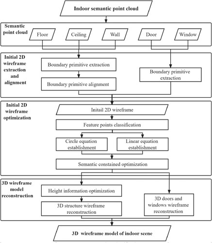
First, the indoor point clouds are classified into six main classes, floors, walls, ceilings, doors, windows, and others with existing point cloud segmentation methods, such as the RandLA-Net (Hu et al. 2020).

Second, alpha-shape-based algorithms are applied to extract the incomplete 2D boundary primitives using semantic point clouds. Afterward, a boundary alignment strategy is applied to obtain the initial 2D boundary. This part can be found in subsection 2.2.

Then, the 2D wireframe’s features are classified based on the contextual relationship. Semantic-constrained feature optimization methods are proposed to optimize the irregular geometry structure. This part can be found in subsection 2.3.

Finally, we reconstruct a 3D wireframe model with a complete and regular geometric structure and actual height change. This part can be found in subsection 2.4.

2.2. Initial 2D wireframe extraction and alignment

This subsection presents a method to generate the initial 2D wireframe from the semantic point cloud.

2.2.1. Boundary primitive extraction

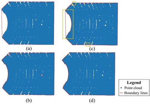
The floor’s point cloud contains abundant features of the indoor scene. However, the occlusions in indoor scenes may cause deficiencies in point clouds. We propose an alpha shape algorithm-based method to detect the boundary primitive from the floor point cloud and fix the primitives missing as possible, such as occlusions caused by objects. Here, two parameters are utilized as the input of the proposed method, namely ${\alpha }_1$ and ${\alpha }_2$, where ${\alpha }_1>{\alpha }_2$. The larger the alpha parameter is, the fewer details the extracted boundary contains. Therefore, a rough boundary primitive could be extracted with the parameter ${\alpha }_1$, shown in Figure 2 (a). A detailed boundary could be extracted with the smaller parameter ${\alpha }_2$, shown in Figure 2 (b). The rough boundary loses some concave structures, and the detailed boundary contains some redundant primitive. We combined the two boundaries’ primitives and generated polygons among the common points. The polygons with these characteristics will be removed from the redundant boundary’s primitives: the area is too small or too large, and rough and detailed primitives are close to overlapping. For example, polygons with an area smaller than 0.05 $m^2$ are considered noise or irregular boundaries from data acquisition. The ratio between a polygon’s area and the area enclosed by the rough boundary determines large-area polygons. Ratios exceeding 5% indicate occlusion-induced missing regions, while ratios exceeding 10% are more likely to suggest concave-shaped structures. Detailed boundary line segments are removed from small, occlusion, and overlapping polygons, while rough boundary line segments are removed from concave-shaped polygons. A clear floor boundary primitive can be generated finally.

Figure 2. Floor boundary primitive extraction. (a) Rough boundary of ${\alpha }_1$. (b) Detailed boundary of ${\alpha }_2$. (c) Illustration of combined polygons. (d) Result of boundary extraction.

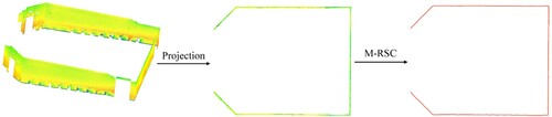
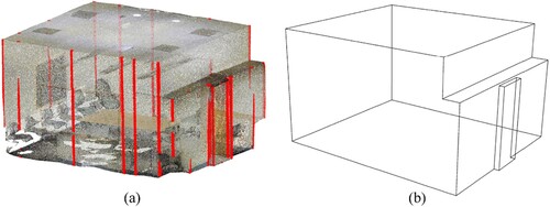
The wall’s point cloud can provide some structural primitives when the floor’s point cloud is too broken to extract a complete boundary. First, we denoised the wall’s point cloud to retain the wall’s structures. The wall point cloud is assumed to be perpendicular to the horizontal plane. Therefore, the wall’s point cloud is projected to a horizontal plane for further extraction. A modified ring-stepping clustering (M-RSC) method (Wu et al. 2021) is applied to extract line segments from the point cloud, as shown in Figure 3.

Figure 3. Wall primitives extraction with the M-RSC method.

In addition, due to the inclusion of height information in the feature points of the ceiling and its relatively complete point cloud with less occlusion, we utilize the alpha shape algorithm to extract the primitives of the ceiling.

2.2.2. Boundary primitive alignment

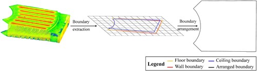
After extracting the boundary primitives, overlapping primitives from different sources necessitates a boundary primitives alignment process to generate a clear boundary. This process is illustrated in Figure 4. All points from the different boundaries are grouped into a pointset. Then, an alpha-shape method is applied to extract the primitives from the pointset. The corner points of ceilings should be saved to extract the height information. Finally, an initial 2D wireframe of an indoor scene can be generated.

Figure 4. Illustration of the boundary primitives alignment.

2.3. Initial 2D wireframe optimization

2.3.1. Feature points classification

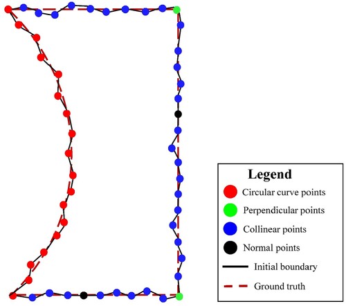
The initial 2D wireframe is rough, with some distortion and irregular features. A semantic-constrained optimization model is proposed to optimize distortion and the irregular geometric structure based on the geometric semantic categories. As Figure 5 shows, the initial boundaries (black lines) consist of many vertices (dots). Before applying the semantic-constrained optimization model, a feature classification method is introduced to classify the feature points into different categories: circular curve points (red dots), perpendicular points (green dots), collinear points (blue dots), and normal points (black dots).

• Circular curve classification

Figure 5. Classification of feature points.

The initial 2D wireframe is divided into polylines to determine the circular curve. Polylines that consist of more than three points are utilized to fit circular curves using the least-squares method, which can determine the center and radius (denoted as $\hat{R}$) of the fitting circular curve. $R_i$ is the distance between feature points on the polyline and the fitted center. First, the polylines with a fitted radius large enough are considered straight lines. Other polylines are estimated by the mean absolute percentage error index (MAPE), shown in Equation (1). (1) $\begin{array}{c}MAPE={\displaystyle \frac{100\text{\%}}{n}\sum _{i=1}^n\left|{\displaystyle \frac{\hat{R}-R_i}{R_i}}\right|}\end{array}$(1) A polyline can be referred to as a circular curve if its MAPE index is smaller than 5%. Furtherly, if the central angle of a fitted circle for a polyline is too small, the polylines are considered non-circular polylines.

• Linear structure classification

Suppose the coordinates of vertices in the initial wireframe are $\left(x_i,y_i\right)$ $\left(i=1,2,\dots ,n\right)$, where $n$ is the number of vertices. Then, the angles of points are calculated with Equation (2). (2) $\begin{array}{c}\{\begin{array}{c}{A}_i={\alpha }_{i,i+1}-{\alpha }_{i,i-1},if{\alpha }_{i,i+1}>{\alpha }_{i,i-1}\\ A_i={\alpha }_{i,i-1}-{\alpha }_{i,i+1},if{\alpha }_{i,i-1}>{\alpha }_{i,i+1}\end{array}\end{array}$(2) where ${\alpha }_{i,j}=\arctan {\displaystyle \frac{y_j-y_i}{x_j-x_i}}$.

The points whose angles satisfy the specific condition shown in Equation (3) will be classified into perpendicular, collinear, and normal points. (3) $\{\begin{array}{c}Perpendicularpoints:\left|A_i-{90}^{\circ }\right|<{\theta }_{1}or\left|A_i-{270}^{\circ }\right|<{\theta }_1\left(A_i\ne {90}^{\circ }or{A}_i\ne {270}^{\circ }\right)\\ Collinearpoints:\left|A_i-{180}^{\circ }\right|<{\theta }_2\left(A_i\ne {180}^{\circ }\right)\\ Normalpoints\end{array}$(3) where ${\theta }_1$ and ${\theta }_2$ are angle classification thresholds.

2.3.2. Initial 2D wireframe optimization model

This section proposes circular curve and linear polyline optimization models individually and combines them to optimize the 2D initial wireframe simultaneously.

• Circular curve feature optimization model

The points of the circular curve should satisfy the circle geometry condition, shown in Equation (4), where $\left(a,b\right)$ is the center of the circular curve and $r$ is the radius. Because the corrected value is small, the observation point is expanded by the Taylor formula to obtain the first term in Equation (5), where $V_{x_i}$ and $V_{y_i}$ are the corrected values of the observation values, and $\delta a,\delta b,\mathrm{a}\mathrm{n}\mathrm{d}\delta r$ are the corrected values of the circle’s parameters. Linearized equations are organized as the conditional optimization equation with parameters point by point, shown in Equation (6), to correct observation values and calculate circle parameters. (4) $\begin{array}{c}{\left(x-a\right)}^2+{\left(y-b\right)}^2=r^2\end{array}$(4) (5) $\begin{array}{c}\left(x_i-a^0\right)V_{x_i}+\left(y_{\mathrm{i}}-b^0\right)V_{y_i}+\left(a^0-x_i\right)\delta a+\left(b^0-y_i\right)\delta b-r^0\delta r+{\displaystyle \frac{1}{2}\left[{\left(x_i-a^0\right)}^2+{\left(y_i-b^0\right)}^2-r^{0^2}\right]=0}\end{array}$(5) (6) $\begin{array}{c}{\mathit{A}}_{1\mathit{i}}{\mathit{V}}_{1\mathit{i}}+{\mathit{B}}_{1\mathit{i}}{\mathit{X}}_1-{\mathit{W}}_{1\mathit{i}}=0\end{array}$(6)

Here, ${\mathit{A}}_{1\mathit{i}}=\left[\left(x_i-a^0\right),\left(y_{\mathrm{i}}-b^0\right)\right]$ is the coefficient matrix of the corrected values, ${\mathit{V}}_{1\mathit{i}}=[V_{x_i},V_{y_i}{]}^T$ is the matrix of the corrected values, ${\mathit{B}}_{1\mathit{i}}=\left[\left(a^0-x_i\right),\left(b^0-y_i\right),-r^0\right]$ is the coefficient matrix of the circle parameters, ${\mathit{X}}_1=[\delta a,\delta b,\delta r{]}^T$ is the vector of the circle parameters, and ${\mathit{W}}_{1\mathit{i}}=\left[-{\displaystyle \frac{1}{2}\left[{\left(x_i-a^0\right)}^2+{\left(y_i-b^0\right)}^2-r^{0^2}\right]}\right]$ is the closure error.

• Linear feature optimization model

(1) Perpendicular condition

In the initial 2D wireframe, there is a non-perpendicular condition consisting of two adjacent lines, as shown in Figure 6(a). The corresponding geometric equation is shown in Equation (7). The matrix representation of the linearized equations is given in Equation (8). (7) $\begin{array}{c}{\displaystyle \frac{Y_i-Y_j}{X_i-X_j}\times {\displaystyle \frac{Y_k-Y_i}{X_k-X_i}=-1}}\end{array}$(7) (8) $\begin{array}{c}{\mathit{A}}_{2\mathit{i}}{\mathit{V}}_{2\mathit{i}}-{\mathit{W}}_{2\mathit{i}}=0\end{array}$(8) Here, ${\mathit{A}}_{2\mathit{i}}=\left[-\left(X_k-X_i\right),-\left(Y_k-Y_i\right),X_k-2X_i+X_j,Y_k-2Y_i+Y_j,X_i-X_j,Y_i-Y_j\right]$ is the coefficient matrix, ${\mathit{V}}_{2\mathit{i}}=[V_{X_j},V_{Y_j},V_{X_i},V_{Y_i},V_{X_k},V_{Y_k}{]}^T$ is the corrected value of the observation points, and ${\mathit{W}}_{2\mathit{i}}=-\left(Y_i-Y_j\right)\left(Y_k-Y_i\right)-\left(X_i-X_j\right)\left(X_k-X_i\right)$ is the closure error.

Figure 6. Illustration of linear feature optimization. (a) Perpendicular condition. (b) Collinear condition.

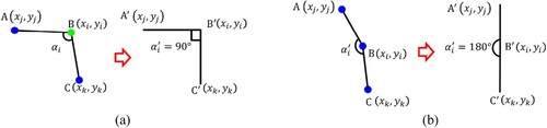
(2) Collinear condition

Figure 6 (b) shows an angle consisting of two adjacent lines slightly different from the flat angle. The two lines are supposed to be the collinear condition and satisfy the geometry given in Equation (9). The matrix representation of the linearized equations is given in Equation (10). (9) $\begin{array}{c}{\displaystyle \frac{Y_i-Y_j}{X_i-X_j}={\displaystyle \frac{Y_k-Y_i}{X_k-X_i}}}\end{array}$(9) (10) $\begin{array}{c}{\mathit{A}}_{3\mathit{i}}{\mathit{V}}_{3\mathit{i}}-{\mathit{W}}_{3\mathit{i}}=0\end{array}$(10) Here, ${\mathit{A}}_{3\mathit{i}}=\left[-\left(Y_k-Y_i\right),\left(X_k-X_i\right),Y_k-Y_j,Y_k-\left(X_k-X_j\right),-\left(Y_i-Y_j\right),X_i-X_j\right]$ is the coefficient matrix, ${\mathit{V}}_{3\mathit{i}}=[V_{X_j},V_{Y_j},V_{X_i},V_{Y_i},V_{X_k},V_{Y_k}{]}^T$ is the small corrected value of the observation points, and ${\mathit{W}}_{3\mathit{i}}=\left(X_i-X_j\right)\left(Y_k-Y_i\right)-\left(X_k-X_i\right)\left(Y_k-Y_i\right)$ is the the closure error.

2.3.3. Irregular point optimization method

To maintain the contextual geometry relationship, simultaneously optimizing all irregular conditions pertaining to other points is essential. Each irregular point is evaluated to determine its relationship with other irregular points. Point groups are organized by considering each irregular point along with its previous and next points. The start node-set and end node-set are determined based on the sequence of point groups. After retrieving all the points, if there is only one start node and one end node, all feature points are optimized together. Otherwise, points between the corresponding start and end nodes are optimized block by block. Different semantic-constrained optimization models are employed in block optimization depending on the presence of a circular curve.

• Semantic-constrained optimization method with linear irregularity

All feature points can be organized as linearized equations based on their specific types if there is merely linear irregularity. Because many linearized equations are arranged one after another, these equations can be enumerated in the following matrix. (11) $\begin{array}{c}\mathit{A}\mathit{V}\mathbf{-}\mathit{W}\mathbf{=}\mathbf{0}\end{array}$(11) (12) $\begin{array}{c}\mathit{W}=AL-{\mathit{A}}_{\mathbf{0}}\end{array}$(12) In this equation, $\mathit{V}$ is the adjusted value of observation, which can be expressed as the vector $[V_{X_1},V_{Y_2},\dots ,V_{X_n},V_{Y_n}{]}^T$. $\mathit{W}$ is the closure error vector, $\mathit{L}$ is the observation vector, and ${\mathit{A}}_0$ is the constant vector of the true value. $\mathit{A}$ is a $\left(n-t\right)\times 2n$ designed matrix, where $n$ is the number of observed points, and $t$ is the number of common points between two irregular points called pseudo common points. Typically, pseudo-common points are corrected twice using the preceding and succeeding irregular parts, or their values are the average of the two optimization results. However, this method may violate geometric constraints and disrupt the continuity of line segments. To address this issue, we propose a combined semantic-constrained optimization method, which corrects pseudo-common points simultaneously using two irregular parts. As a result, the corrected pseudo-common points can satisfy the requirements of both geometric structures. Here, $\mathit{A}$ is an approximate block diagonal matrix shown in Equation (13). In this matrix, $\mathit{O}$ is the zero matrix. The parameter matrices ${\mathit{A}}_{\mathit{i}}$ and ${\mathit{A}}_{\mathit{i}+1}$ are enumerated as the form of Equation (14). However, if there is a pseudo-common point between ${\mathit{A}}_{\mathit{i}}$ and ${\mathit{A}}_{\mathit{i}+1}$, the enumerated form will take the change shown in Equation (15). (13) $\begin{array}{c}\mathit{A}=\left[\begin{array}{ccc}{\mathit{A}}_{\mathbf{1}}& \cdots & \mathit{O}\\ ⋮& \ddots & ⋮\\ \mathit{O}& \cdots & {\mathit{A}}_{\left(\mathit{n}-\mathit{t}\right)}\end{array}\right]\end{array}$(13) (14) $\begin{array}{c}\left[\begin{array}{cccccccc}{a}_{i,1}& a_{i,2}& a_{i,3}& a_{i,4}& a_{i,5}& a_{i,6}& 0& 0\\ 0& 0& a_{i+1,1}& a_{i+1,2}& a_{i+1,3}& a_{i+1,4}& a_{i+1,5}& a_{i+1,6}\end{array}\right]\end{array}$(14) (15) $\begin{array}{c}\left[\begin{array}{cccccccccc}{a}_{i,1}& a_{i,2}& a_{i,3}& a_{i,4}& a_{i,5}& a_{i,6}& 0& 0& 0& 0\\ 0& 0& 0& 0& a_{i+1,1}& a_{i+1,2}& a_{i+1,3}& a_{i+1,4}& a_{i+1,5}& a_{i+1,6}\end{array}\right]\end{array}$(15)

Finally, the corrected value vector $\mathit{V}$ can be calculated as follows: (16) $\begin{array}{c}\mathit{V}={\mathit{P}}^{-1}{\mathit{A}}^{\mathit{T}}{\left(\mathit{A}{\mathit{P}}^{-1}{\mathit{A}}^{\mathit{T}}\right)}^{-1}\mathit{W}\end{array}$(16) Here, $\mathit{P}$ represents the weight matrix of observation values determined by each observation’s condition. If all observations have the same condition, $\mathit{P}$ is an identity matrix. In our case, $\mathit{P}$ is set as an identity matrix.

• Semantic-constrained optimization method with the circle curve and linear irregularity

The circular curve could occur alone or be connected with linear structures in the indoor scene. Despite having different geometric conditions, their general matrices follow the same format. The observation points can be enumerated in matrix format as follows. (17) $\begin{array}{c}\mathit{A}V+BX-W=0\end{array}$(17) Equation (5) states that a circular curve has three unknown parameters. A semantic-constrained optimization method with parameters determines the observed and parameter-corrected values.

If the circular curve occurs alone, all points will be enumerated in the form of Equation (17). Under this condition, $\mathit{V}$ is a $2n$ designed corrected value vector of observation points on the circular curve. $\mathit{B}$ is $[{\mathit{B}}_1,{\mathit{B}}_2,\dots ,{\mathit{B}}_{\mathit{n}}{]}^{\mathit{T}}$, which is an $n\times 3$ designed coefficient matrix of unknown parameters, where ${\mathit{B}}_{\mathit{i}}$ is the coefficient vector of each point based on Equation (6). $\mathit{W}$ is a constant vector with the same form as Equation (12). $\mathit{X}$ is a column vector with three elements, including $\delta a,\delta b,\mathrm{a}\mathrm{n}\mathrm{d}\delta r$. $\mathit{A}$ is the $n\times 2n$ designed block diagonal matrix shown in Equation (18), where ${\mathit{A}}_{\mathit{i}}$ is the coefficient matrix of the circular curve conditional equation shown in Equation (6). $n$ is the number of observation points. (18) $\begin{array}{c}\mathit{A}=\left[\begin{array}{ccc}{\mathit{A}}_{\mathbf{1}}& \cdots & \mathit{O}\\ ⋮& \ddots & ⋮\\ \mathit{O}& \cdots & {\mathit{A}}_{\mathit{n}}\end{array}\right]\end{array}$(18) If the circular curve concatenates with linear geometry components, $\mathit{B}$ has the same format as the condition of the circular curve occurring alone and has $m$ elements. Under this condition, $n$ is the total number of observation points of circle curves and linear structures. To provide a clear illustration, we assume there are $m$ circular curve points and linear structure points and that $m$ plus $t$ equals $n$. The circular curve and linear structure coefficient matrices are combined and enumerated based on their sequence of appearance to optimize two types of geometry conditions. The example that two different categories of geometric structures occurring together are taken as follows. A concatenated matrix is shown as follows, where ${\mathit{A}}_{\mathit{c}}$ is the coefficient matrix of the circular curve, which is the same as that in Equation (18), and ${\mathit{A}}_{\mathit{l}}$ is the coefficient matrix of the linear structure, which is the same as that in Equation (13). Similarly, ${\mathit{V}}_{\mathit{t}otal}$ and ${\mathit{W}}_{\mathit{t}otal}$ are composed of vectors representing the two categories of geometric structures, shown in Equation (20). (19) $\begin{array}{c}{\mathit{A}}_{\mathit{t}otal}=\left[\begin{array}{cc}{\mathit{A}}_{\mathit{c}}& \mathit{O}\\ \mathit{O}& {\mathit{A}}_{\mathit{l}}\end{array}\right]\end{array}$(19) (20) $\begin{array}{c}{\mathit{V}}_{\mathit{t}otal}=\left[\begin{array}{c}{\mathit{V}}_{\mathit{c}}\\ {\mathit{V}}_{\mathit{l}}\end{array}\right]{\mathit{W}}_{\mathit{t}otal}=\left[\begin{array}{c}{\mathit{W}}_{\mathit{c}}\\ {\mathit{W}}_{\mathit{l}}\end{array}\right]\end{array}$(20) After constructing the combined matrix and vector, the parameter vector and corrected value vector solutions can be calculated as follows. (21) $\begin{array}{c}\mathit{X}={\left[{\mathit{B}}^{\mathit{T}}{\left({\mathit{A}}_{\mathit{t}otal}\mathit{P}{\mathit{A}}_{\mathit{t}otal}{}^{\mathit{T}}\right)}^{-1}\mathit{B}\right]}^{-1}{\mathit{B}}^{\mathit{T}}{\left({\mathit{A}}_{\mathit{t}otal}\mathit{P}{\mathit{A}}_{\mathit{t}otal}{}^{\mathit{T}}\right)}^{-1}{\mathit{W}}_{\mathit{t}otal}\end{array}$(21) (22) $\begin{array}{c}{\mathit{V}}_{\mathit{t}otal}=\mathit{P}{\mathit{A}}_{\mathit{t}otal}{}^{\mathit{T}}\left[-{\left({\mathit{A}}_{\mathit{t}otal}\mathit{P}{\mathit{A}}_{\mathit{t}otal}{}^{\mathit{T}}\right)}^{-1}\left(\mathit{B}X-{\mathit{W}}_{\mathit{t}otal}\right)\right]\end{array}$(22) Here, $\mathit{P}$ is an identity matrix which is the weight matrix of observation values. Moreover, if there are more than two continuous structures in one region restrained by a starting point and a corresponding endpoint, we can enumerate them in matrices successively according to Equation (19) and Equation (20) and calculate the solution by using Equation (21) and Equation (22).

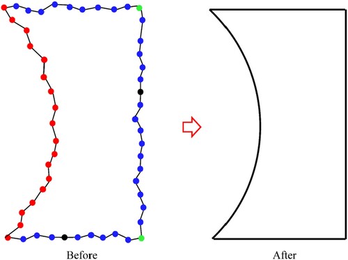
An iteration method is utilized to optimize the initial feature points shown in Figure 7. The corresponding geometry conditions are solved using Equation (16) and Equation (22) in the first iteration. The solution is compared with the original coordinates and is used to calculate three indicators of iteration convergence, $\mathrm{\Delta }x$, $\mathrm{\Delta }y$, and $\mathrm{\Delta }pt$, which are the difference values of the x coordinate, the y coordinate, and the point, respectively. If these indicators do not satisfy the convergence thresholds, the corrected feature points are reclassified, and the iteration steps are repeated. By iteration, a geometrically correct 2D wireframe can be generated when all indicators are satisfied. The comparison of the initial 2D wireframe and the optimized 2D wireframe is shown in Figure 8.

Figure 7. Pipeline of the iterative semantic constrained optimization method.

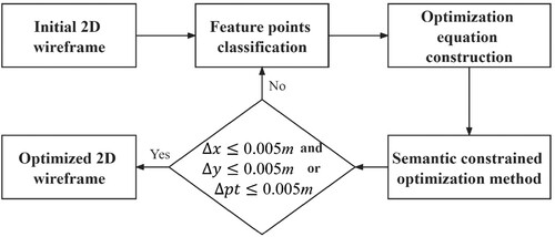
Figure 8. Comparison between the initial 2D wireframe and optimized 2D wireframe.

2.4. 3D wireframe model reconstruction

2.4.1. Door and window wireframe reconstruction

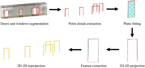
We introduce a method for extracting the wireframe of doors and windows whose pipeline is shown in Figure 9. First, the plane is fitted by the eigenvalue method from the original points. Points whose distance between the plane and themselves is larger than double the standard deviation are removed. The final plane is determined when all remaining points are below the threshold. By using the plane equation, points of doors and windows are projected onto a 2D plane. The alpha shape method is then utilized to extract the feature points, which will be subsequently categorized. The semantic-constrained optimization method is applied to regularize the feature points. Finally, the optimized points are reprojected into 3D space to generate the doors and windows’ 3D wireframes, as shown in Figure 9.

Figure 9. Pipeline of door and window wireframe extraction.

2.4.2. 3D structure wireframe reconstruction

The height information is necessary for feature points to reconstruct a 3D wireframe. The heights of feature points are extracted with point cylinders, as shown in Figure 10. Points whose distance to the feature points is smaller than the threshold, usually 2.5 centimeters, are gathered within the cylinder. The highest point, which exhibits no significant height difference from the second-highest point, is assigned the top height for the feature points. The bottom heights of feature points are extracted similarly. However, some abnormal heights impact the vertical structure, which is shown in Figure 11(a).

Figure 10. Illustration of height information extraction. (a) Schematic diagram of the cylinder method. (b) Example of height extraction by the cylinder method.

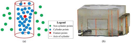
Figure 11. Height information optimization. (a) Abnormal height. (b) Height undulation. (c) Corrected abnormal height. (d) Smooth height edges.

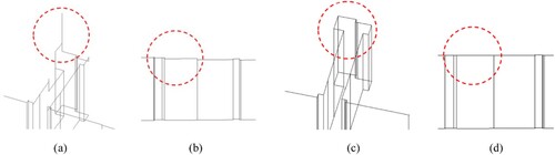
A height distribution histogram is counted from the point cloud, as shown in Figure 12. The height ranges with significant differences are identified based on the statistical analysis. For heights within a specific range, the weighted average is calculated and assigned as the reference for height, denoted as $h_{ref}$. To further smooth the heights, neighboring heights are considered. If a point’s height significantly deviates from its neighboring points, it is corrected to the nearest value between the two neighboring heights. The corrected height is shown in Figure 11 (c). However, some slight undulation may persist, as shown in Figure 11 (b). The bottom and top heights of feature points are adjusted to match the corresponding reference heights, provided that the difference between the reference height and the original height is below a threshold, usually within 5 centimeters, shown in Figure 11 (d).

Figure 12. Reference height extraction by a height histogram. (a) Histogram of the height distribution of points. (b) Corresponding plane detected by the histogram.

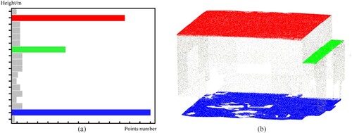
Once the height information is determined, the feature points’ 3D coordinates can be determined. It allows for the reconstruction of the 3D model in three steps. First, the feature points on the floor are connected from point to point, forming the indoor scene’s floor structure. Similarly, the ceiling’s feature points are also connected based on height. Finally, the vertical wall line segment is generated for the corner points. The door and window wireframes are placed on the wall based on their coordinates to express the connectivity of the indoor scene. The result of height information extraction and 3D wireframe reconstruction is shown in Figure 13.

Figure 13. Height information extraction and reconstruction. (a) Height information in the point cloud. (b) Reconstruction structure from height information.

3. Experiments and results

3.1. Data preparation

This study verifies our method using three public benchmark datasets captured by different devices and institutions. The three benchmark datasets are the Stanford 2D–3D-Semantics dataset (Scene 1) (Armeni et al. 2017), the ISPRS benchmark on multisensorial indoor mapping and positioning (Scene 2) (Wang et al. 2018; Wen et al. 2020). and the International Society for Photogrammetry and Remote Sensing (ISPRS) benchmark dataset (Scene 3) (Khoshelham et al. 2017). The experimental datasets contain typical indoor scenes of different scales, precision, and geometric structures.

A long corridor is selected as Scene 1, representing a long and narrow scene with many doors and windows, which is used to trial the ability to reconstruct opening areas.

Due to the full semantic element and many variations in the vertical direction, Scene2 is selected to test and compare our method with other methods. This indoor scene contains a corridor and multiple rooms with high clutter and missing structures.

In addition, Scene 3 is selected to reconstruct the 3D wireframe and evaluate accuracy quantitively. This scene consists of 13 rooms and has high clutter caused by many showpieces. This scene has many curves and changes in height. Due to the scenario complexity and comprehensive structure categories, it’s challenging to reconstruct an accurate 3D wireframe. The comprehensive structures, including linear and circular structures and abundant height changes, can provide abundant evaluation samples for the proposed method.

We used RandLA-Net to finish the semantic segmentation and segment the point cloud into six semantic categories: floor, wall, ceiling, doors and windows, and others Table 1 and Figure 14.

Figure 14. Three experimental scenes.

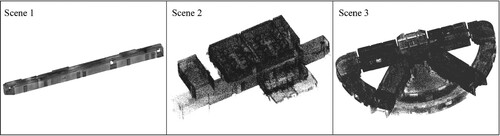
Table 1. Data description of testing scenes.

Indoor scene	Scene 1	Scene 2	Scene 3
Source	S3DIS Dataset	ISPRS Dataset	ISPRS Dataset
Category	Long Corridor	Multiroom	Granger Museum
Characteristic	Long and narrow, many doors and windows	High clutter with a height change	High clutter and complex
Point number	4481021	8688375	23517095
Clutter	Low	Medium	High
Area ($m^2$)	88.882	238.996	2020.340

3.2. Parameters setting and accuracy evaluation indices

3.2.1. Parameters setting

All the experiments in the three scenes are implemented using a laptop with an AMD Ryzen 7 5800H processor, an NVIDIA 3060 laptop with 16 GB of memory, and a Windows operating system.

Here, the parameters for primitives’ extraction are introduced as follows. During the initial wireframe extraction, two parameters, namely ${\alpha }_1$ and ${\alpha }_2$ are used to extract the floor’s boundary primitives. The values of these two parameters are listed in Table 2. Referring to Wu et al.’s work (Wu et al. 2021), the parameters for the wall’s primitive boundary extraction are listed in Table 3. Due to the fewer attachments and less occlusion, the ceiling point clouds are completer than the floor point clouds. Therefore, we set the alpha shape’s ceiling parameters to be 0.08–0.1 m for most indoor scenes. In addition, the parameters for doors and windows extraction are set as an extremely large value to capture the corners and reduce fragmented details, such as 200 m.

Table 2. Parameters for floor boundary extraction.

Indoor scene	Scene 1	Scene 2	Scene 3
${\mathit{\alpha }}_1$(m)	15	15	15
${\mathit{\alpha }}_2$(m)	0.1	0.1	0.1

Table 3. Parameters for wall boundary extraction.

Indoor scene	Scene 1	Scene 2	Scene 3
R	0.03	0.05	0.03
$N_{stop}$	5	15	10

Section 2.3 uses some thresholds to classify the feature points and control the iteration process. A couple of linear feature classification threshold ${\theta }_1$ and ${\theta }_2$ are set to $5^{\circ }$. Smaller thresholds can only capture a limited number of irregular phenomena in the scene, while a larger threshold increases the likelihood of misclassification and non-convergence during the iterative process. To avoid or reduce overfitting optimization and non-convergence, we set the termination thresholds as follows: $\mathrm{\Delta }x=0.005m$ and $\mathrm{\Delta }y=0.005m$, or $\mathrm{\Delta }pt=0.005m$, and the maximum iteration number is five.

3.2.2. Accuracy evaluation indices

To evaluate the accuracy of the reconstructed 3D wireframe model, we utilized three evaluation indices to evaluate the performance of our model. The schematic diagram of the methods of evaluation is shown in Figure 15.

Figure 15. Three indicators of accuracy evaluation.

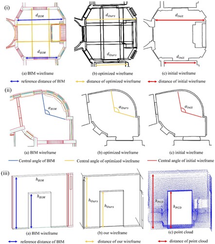
The first evaluation indicator is planar accuracy, which refers to Yang et al.’s work (Yang et al. 2019) and is shown in Equation (23). It calculates the planar distance and curves’ length from structures. $\mathrm{\Delta }{d}_{Ours}^i$ denotes the distance difference between our wireframe and BIM, while $\mathrm{\Delta }{d}_{Init}^i$ denotes the distance difference between the initial wireframe and BIM.

The second indicator is the central angle for evaluating the circular curves, which is shown in Equation (24). The central angles are calculated based on the arc length and radius of circular curves. The arc length and radius of the curves are calculated from the optimized and initial wireframes. $\mathrm{\Delta }{\alpha }_{Ours}^i$ denotes the angle difference between our wireframe and BIM, while $\mathrm{\Delta }{d}_{Init}^i$ denotes the angle difference between the initial wireframe and BIM.

Thirdly, the height difference is utilized to evaluate the 3D reconstruction accuracy, which is shown in Equation (25). The heights of the corresponding position from BIM, our wireframe, and the original point cloud are used to evaluate the height accuracy. Considering that our wireframe’s 3D information is extracted from the point cloud, the point cloud’s height is set as the comparison’s foundation. The height differences between the BIM and our wireframe are denoted by $\mathrm{\Delta }{h}_{BIM}^i$, while the height differences between the original point cloud and our wireframe are denoted by $\mathrm{\Delta }{h}_{BIM}^i$. (23) $\begin{array}{c}\{\begin{array}{c}{d}_{BIM}^i=P_{BIM}^j-P_{BIM}^k\\ d_{Ours}^i=P_{Ours}^j-P_{Ours}^k\\ d_{Init}^i=P_{Init}^j-P_{Init}^k\end{array},\{\begin{array}{c}\mathrm{\Delta }{d}_{Ours}^i=\left|d_{BIM}^i-d_{Ours}^i\right|\\ \mathrm{\Delta }{d}_{Init}^i=\left|d_{BIM}^i-d_{Init}^i\right|\end{array}\end{array}$(23) (24) $\begin{array}{c}\alpha ={\displaystyle \frac{s}{2\pi R}\ast {360}^{\circ },\{\begin{array}{c}\mathrm{\Delta }{\alpha }_{Ours}^i=\left|{\alpha }_{BIM}^i-{\alpha }_{Ours}^i\right|\\ \mathrm{\Delta }{\alpha }_{Init}^i=\left|{\alpha }_{BIM}^i-{\alpha }_{Init}^i\right|\end{array}}\end{array}$(24) (25) $\begin{array}{c}\{\begin{array}{c}{h}_{BIM}^i=P_{BIM}^j-P_{BIM}^k\\ h_{Ours}^i=P_{Ours}^j-P_{Ours}^k\\ h_{PCD}^i=P_{PCD}^j-P_{PCD}^k\end{array},\{\begin{array}{c}\mathrm{\Delta }{h}_{BIM}^i=\left|h_{BIM}^i-h_{PCD}^i\right|\\ \mathrm{\Delta }{h}_{Ours}^i=\left|h_{Ours}^i-h_{PCD}^i\right|\end{array}\end{array}$(25)

3.3. Initial 2D wireframe extraction and optimization

3.3.1. Initial 2D wireframe results

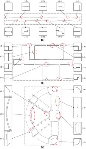
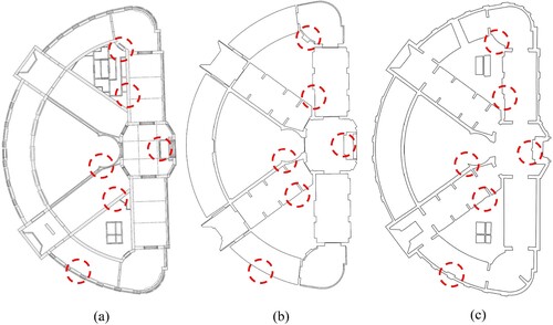
After aligning all boundary primitives, the initial 2D wireframes of the experimental scenes are shown in Figure 16, which highlights the irregularities in the initial wireframes. The initial results fail to achieve geometric consistency and accuracy in the structure. The analysis is summarized as follows.

Figure 16. Initial 2D wireframe of experimental scenes. (a) Scene 1. (b) Scene 2. (c) Scene 3.

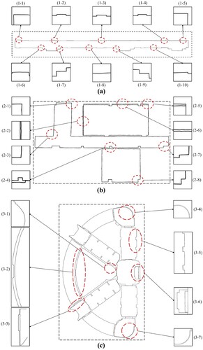
Scene 1 is a long and narrow corridor with many perpendicular and colinear structures. However, due to the quality of the scan, there are some noticeable protrusions where the walls should be straight, such as in (1–8). Additionally, the corners of the rectangular room are not perfectly perpendicular, as seen in (1–1) and (1–5). Furthermore, because of the susceptibility to edge noise during primitive extraction, the extracted boundaries may exhibit slight irregular deformations, as shown in (1–2) and (1–3).

Scene 2 comprises multiple rooms and a corridor and presents three primary irregularities. Firstly, small deformations result in deviations from straight lines caused by the point cloud thickness, as observed in (2–4). Secondly, due to scan quality, non-perpendicular corners are observed in (2–3) and (2–8). Lastly, a lack of parallelism is observed between two straight lines that should be parallel, as in (2–2) and (2–6). In this scene, preserving the parallel or tangent relationships between rooms during optimization is crucial for achieving good results.

Scene 3 is a large, complex environment encompassing various linear and circular structures. In addition to the above phenomena, two primary concerns need to be addressed in relation to circular structures. Firstly, the circular curves in the scene exhibit slight undulations along their edges, which can be observed in (3–1). Secondly, the curves of the concentric circles in the scene are not parallel, as is evident in (3–2) and (3–4).

3.3.2. Initial wireframe optimization

Because of the above phenomena, the initial 2D wireframe should be optimized to advance geometric consistency and accuracy.

The optimized 2D wireframes are shown in Figure 17, demonstrating significant geometric and semantic consistency improvements. For Scene 1, we successfully overcame the challenges brought about by the abundant and continuous irregular structures through our optimization method. The collinear and perpendicular structures of the walls were restored well. For Scene 2, the parallel walls were adjusted to their correct relationship, and adjacent rooms were nearly parallel or tangent after optimization. The optimization method effectively avoided local over-optimization and geometric deformation. In Scene 3, the geometric structure of multiple rooms was reconstructed successfully. We focused on optimizing the circular curve structures in addition to the linear ones. The circular curves with slight undulations were smoothed out, and the concentric circles’ circular curves were restored to their parallel relationship.

Figure 17. Optimized 2D wireframe of experimental scenes. (a) Scene 1. (b) Scene 2. (c) Scene 3.

3.4. 3D wireframe model reconstruction

The floor and ceiling height values are applied to feature points to generate the 3D feature points. Using the categories and the 3D coordinates of feature points, we can reconstruct scenes with three basic structures: floors, walls, and ceilings. Doors and windows are reconstructed from corresponding semantic point clouds and placed on basic structures to reconstruct a complete indoor scene. The effectiveness of our method in reconstructing structures is demonstrated by the 3D wireframes of experimental scenes in Figures 18–20.

Figure 18. 3D wireframes of Scene 1. (a) 3D wireframe with semantics. (b) Details of doors and windows.

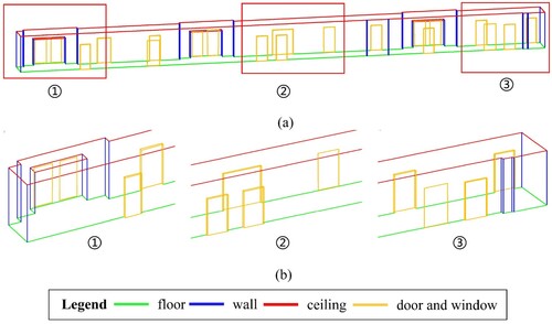
Figure 19. 3D wireframe of Scene 2.

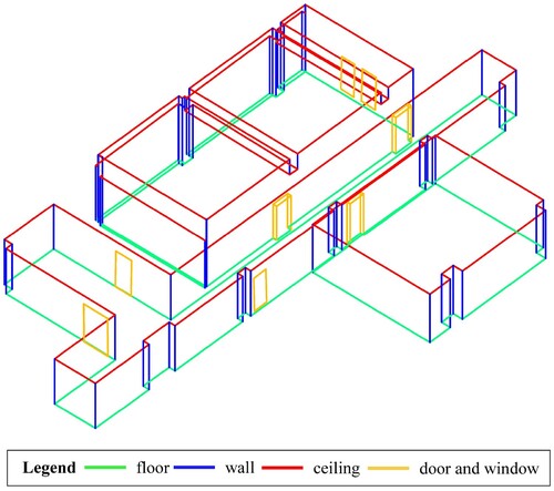
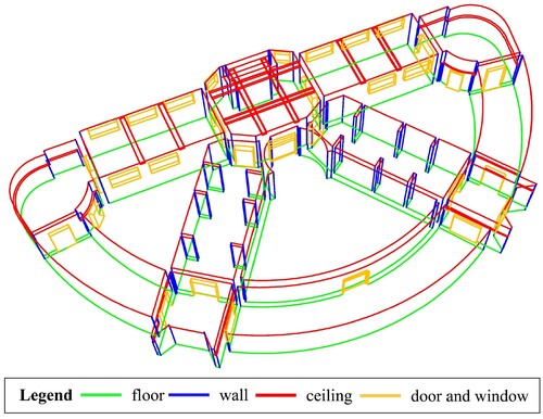
Figure 20. 3D wireframe of Scene 3.

Scene 1 is a long, narrow corridor featuring multiple doors and windows with uneven heights, including some low doorcases. Our focus in this scene was to test the ability of our method to reconstruct opening areas. The details of opening areas are illustrated in Figure 18 (b), where all doors and windows are reconstructed on the surface of the walls. With the semantic-constrained optimization method, the geometric structures of the opening areas were accurately reconstructed. The 3D reconstruction method based on feature points effectively reconstructed the uneven heights, and low doorcases were reconstructed correctly.

Scene 2 is a multi-room environment with walls of uneven width on the upper and lower levels and local depressions on the ceiling caused by crossbeams. These characteristics constitute a structurally complex indoor scene. Due to the multi-source feature points extraction, uneven width of walls and the crossbeams can be extracted and reconstructed. In addition, the doors and windows are reconstructed in the correct place. Different rooms are closely adjacent without spatial conflict.

Scene 3 is a comprehensive scenario that contains circular curves, uneven heights, and opening areas. In Scene 3, the height difference between the inner and outer walls and the height changes caused by the ceiling structure were well reconstructed. Doors between two adjacent rooms are parallel or tangential. After processing with the proposed method, a clear, semantically accurate 3D wireframe is reconstructed.

3.5. Accuracy evaluation and analysis

In this subsection, the accuracy of our method is evaluated quantitatively. Considering the characteristics of our method, the effectiveness is evaluated through three aspects: geometric accuracy of the planar structure, extracted height, and circular curves. The BIM from the ISPRS dataset is used as the reference.

Table 4 presents the averages of the three evaluation indicators for Scene 3, while Figure 21 illustrates the corresponding broken line graphs. Regarding planar structures, our method demonstrates improved accuracy in most conditions, resulting in an average accuracy improvement of 20%. However, in certain cases, there may be structures where the optimization made by the excessive threshold or number of iterations results in less accurate outcomes.

Figure 21. Distribution of the accuracy evaluation. (a) Planar accuracy. (b) Curve accuracy. (c) Height accuracy.

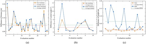
Table 4. Average of evaluation indicators.

Indicator1	$\mathrm{\Delta }d$(m)	Improvement
Our wireframe	0.044	20%
Initial wireframe	0.055
Indicator2	$\mathrm{\Delta }\alpha {(}^{\circ })$	Improvement
Our wireframe	2.197	33.3%
Initial wireframe	3.298
Indicator3	$\mathrm{\Delta }h$(m)	Improvement
Our wireframe	0.008	87.7%
BIM	0.065

The central angle reflects the accuracy of the circular curves. Our method can improve the geometric circle curves by approximately 33.3% on average. It effectively corrects distortions in circular curves that have significant deviations. For the relatively accurate circular curves, due to the combined optimization strategy, it would not cause local over-fitting.

In height evaluation, our method successfully extracts heights that closely align with the point cloud data, with differences limited to the millimeter level. However, two phenomena are observed when comparing the point cloud with the BIM. Firstly, some experimental samples, particularly components such as doors and windows, exhibit differences close to the centimeter level. This demonstrates the accurate 3D reconstruction capability of the proposed method. Secondly, the average height difference for ceilings is primarily at the decimeter level. This difference can be attributed to additional structural elements present in the ceiling, which may cause a bias between the point cloud and the designed BIM.

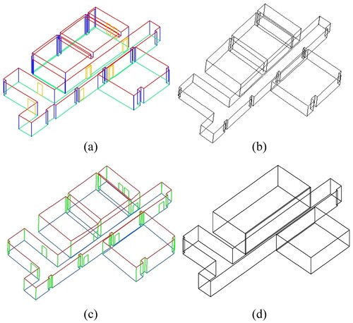
3.6. Comparison with existing methods

To elucidate the advancement and efficacy of the proposed method, we conduct a comparison analysis with four methods qualitatively and quantitatively (Han et al. 2021; Oesau, Lafarge, and Alliez 2014; Wang et al. 2018; Wu et al. 2021). These methods include classical and state-of-art methods and are divided into 2D and 3D wireframe reconstruction. H. Wu et al. proposed a 2D method that extracted linear and curve primitives from sliced wall point clouds and optimized them by a local least-square model. Other methods focused on 3D wireframe reconstruction. Oesau et al. extracted and optimized indoor wireframes with a graph cut from the point cloud. Wang et al. directly extracted line segments from point clouds and reconstructed the 3D wireframe with semantics and height changes. Han et al. segmented rooms with graph theory and reprojects primitives to the original plane to generate a 3D model with actual height.

3.6.1. Qualitative analysis

The 2D wireframe comparison is shown in Figure 22. Compared to Wu et al.’s method, our wireframes exhibit superior optimization performance in structural refinement, resulting in more regular and smooth boundaries by employing a combined optimization strategy.

Figure 22. 2D Method comparison on Scene 3. (a) BIM. (b) our method. (c) Wu et al.’s method.

The 3D wireframe comparison is shown in Figure 23. Compared to Oesau et al.’s method, our method exhibits advantages regarding semantic attribute extraction and accurate height reconstruction of the structures. Compared to Wang et al.’s method, by extracting primitives from multi-sources point clouds, our method captures more details effectively, such as the interior and exterior boundaries of the upper room. Han et al.’s method successfully reconstructed the individual rooms’ heights, but the excessive segmentation resulting from cell decomposition affected the integrity reconstruction of the internal and boundary structures of the rooms, where our method performed well.

Figure 23. 3D Method comparison on Scene 2. (a) Our method. (b) Oesau et al.’s method. (c) Wang et al.’s method. (d) Han et al.’s method.

3.6.2. Quantitative analysis

To provide a more comprehensive assessment of various methods, we analyzed the position error of points, which is calculated as Equation (26). Here,$x_i,y_i,z_i$ are the wireframes’ points coordinates, and $X_i,Y_i,Z_i$ are the reference’s coordinates. Specifically, we selected a series of corresponding points from the reconstructed wireframes and the measurement reference. (26) $\begin{array}{c}\{\begin{array}{c}3Dconditions:{\displaystyle \frac{{\sum }_{i=1}^N\sqrt{{\left(x_i-X_i\right)}^2+{\left(y_i-Y_i\right)}^2+{\left(z_i-Z_i\right)}^2}}{N},,i=1,2,\dots ,N}\\ 2Dconditions:{\displaystyle \frac{{\sum }_{i=1}^N\sqrt{{\left(x_i-X_i\right)}^2+{\left(y_i-Y_i\right)}^2}}{N},i=1,2,\dots ,N}\end{array}\end{array}$(26) For Scene 2, the point cloud is set as the reference. Based on the abundant level of reconstructed structures, we pick up 43, 36, and 19 points from our wireframe, Wang et al.’s wireframe, and Han et al.’s wireframe. The position error of points is shown in Table 5.

Table 5. The position error of points of Scene 2.

Method	Ours	Wang et al.’s	Han et al.’s
Position error(m)	0.050	0.211	0.142

For Scene 3, a BIM provided with the dataset is set as the reference. We pick up 82 and 76 points from our wireframe and Wu et al.’s wireframe. The position error of points is shown in Table 6.

Table 6. The position error of points of Scene 3.

Method	Ours	Wu et al.’s
Position error(m)	0.069	0.087

Based on the tables above, our wireframes outperform the comparison methods in Scene 2 and Scene 3. It indicates that the proposed semantic-constrained combined optimization model exhibits superior accuracy in indoor wireframe reconstruction.

4. Discussion

(1) The impact of semantics segmentation method for 3D reconstruction.

In general, many semantic segmentation methods can be used to finish this process. The RandLA-net is chosen in this paper because of its advantage of process efficiency, local feature utilization, and segmentation accuracy (Guo et al. 2020). When the segmentation results occur error segmentation, since the semantic point clouds required in this paper are mostly faceted point clouds with fixed normal vectors, super voxel segmentation and region growing method can be used to aggregate various semantic point clouds further and reduce the impact of error segmentation on graph element extraction, which is shown in Figure 24.

Figure 24. Semantic segmentation results optimization. (a) semantic point cloud with error segmentation. (b) semantic segmentation point cloud after processing.

(2) Optimal parameter selection for initial wireframe extraction

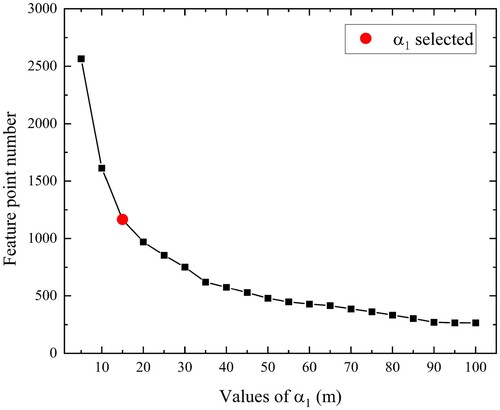
The ${\alpha }_1$ aims to extract the rough boundary of the floor and skip various deficiencies. To determine the suitable parameters, we tested the values of ${\alpha }_1$ from 5 to 100. The corresponding feature points number is shown in Figure 25. The trend of decreasing the number of feature points has changed before and after the value of 15 m. To balance the convex hull’s details and the ability of the ability to fill in occlusion, we selected 15 m as the value of ${\alpha }_1$. The ${\alpha }_2$ aims to capture the details of boundary. All scenes’ average point spacing value in our experiments is 0.012 m. Considering the average value and the maximum distance between neighbor points, we selected 0.1 m as the value of ${\alpha }_2$. The parameters selection is empirical and practical and can be further adjusted based on the practical datasets.

Figure 25. Illustration of ${\alpha }_1$ selection.

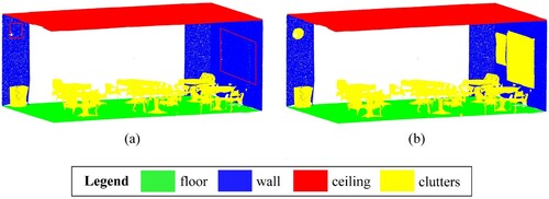
(3) The impact of different categories of ceiling structures on 3D wireframe reconstruction

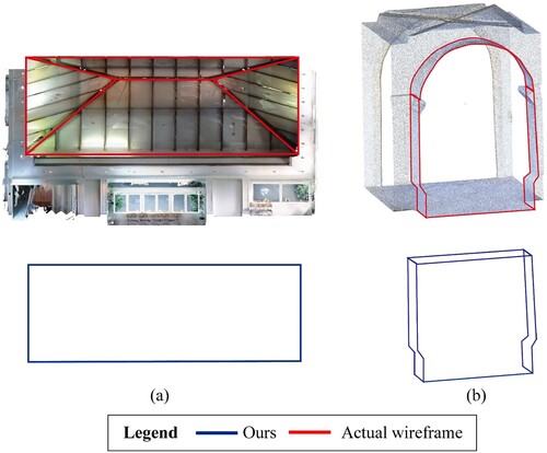
The proposed method performs well in reconstructing horizontal ceilings with varying heights and sloping ceilings. However, the proposed method still cannot reconstruct some non-horizontal structures. Due to the optimization of this method mainly on the edges, the points inside the ceiling are not considered, and it is difficult to reconstruct the sloping roof that bulges in the middle of the building, which can be seen in Figure 26 (a). In addition, because the point cloud of the ceiling is projected on a horizontal plane, some 3D features cannot be detected or will be discrete. This condition will fail to reconstruct the correct 3D structure, such as curved roofs shown in Figure 26 (b).

Figure 26. Illustration of non-horizontal structure. (a) the sloping roof that bulges in the middle of the building. (b) curved roofs.

5. Conclusion

In this study, we proposed a novel method to reconstruct a 3D wireframe from point clouds. Compared with similar previously proposed methods, our method not only extracted and optimized linear features of point clouds but also became suitable for curves and smoothly restored the height of scenes. Our method is tested on three different indoor scenes and evaluated quantitatively.

The main conclusions drawn are as follows:

1. The proposed multi-sources primitive extraction method can fix the deficiency caused by occlusion. Due to the multi-sources feature points, implicit height change can be captured from the point cloud. Compared with other methods, the proposed method can provide more details.

2. The semantic-constrained optimization method can optimize the structure based on its geometric semantics for the irregularity and the missing geometric semantic consistency issue. By iterating, the primitives can be corrected to parallel, perpendicular, and circular. The proposed method optimized the local geometric structure and considered the geometric context relationship, maintaining the whole scene’s consistency and integrity.

3. Reconstruction experiments show the effectiveness of our method. The proposed method can reconstruct 3D semantic wireframes with actual height and semantics. Compared with a designed BIM, the accuracy can be improved by approximately 20% to 33% in different aspects. The high accuracy and abundant semantics can contribute to the indoor scene digital representation.

Considering the limitation and conclusion, the proposed method can be further improved in future work. The multi-room and multi-story connectivity building reconstruction should be considered. This paper focuses on the structure of 3D wireframe. Combined with room plan segmentation and connectivity detection, the indoor scene will be complete and highly accurate in geometric, semantic, and topology, providing high-quality data for building applications. In addition, the optimization method should be expanded to vertical aspects or 3D lines to reconstruct more complex structures.

Data and codes availability statement

The experimental data of ISPRS benchmark on multisensorial indoor mapping and positioning is openly available at http://mi3dmap.net/, S3DIS is available at http://buildingparser.stanford.edu/dataset.html. The code please contact the author Junyi Wei ([email protected]) if needed.

Acknowledgements

Thanks to all authors for their contributions to this article, anonymous reviewers and editors for their valuable comments on the manuscript.

Disclosure statement

No potential conflict of interest was reported by the author(s).

Additional information

Funding

This work was supported by the National Key Research and Development Program of China (Grant No. 2021YFB2501103), the National Science Foundation of China (Grant No. 42271429 and 42130106). the Key Research and Development Projects of Shanghai Science and Technology Commission (Grant No. 21DZ1204103).

References

- Ai, Mengchi, Zhixin Li, and Jie Shan. 2021. “Topologically Consistent Reconstruction for Complex Indoor Structures from Point Clouds.” Remote Sensing 13 (19): 3844. https://doi.org/10.3390/rs13193844.
- Armeni, Iro, Sasha Sax, Amir R Zamir, and Silvio Savarese. 2017. “Joint 2D-3D-semantic Data for Indoor Scene Understanding.” arXiv preprint arXiv:1702.01105. https://doi.org/10.48550/arXiv.1702.01105.
- Barazzetti, Luigi. 2016. “Parametric as-Built Model Generation of Complex Shapes from Point Clouds.” Advanced Engineering Informatics 30 (3): 298–311. https://doi.org/10.1016/j.aei.2016.03.005.
- Bassier, Maarten, and Maarten Vergauwen. 2020. “Unsupervised Reconstruction of Building Information Modeling Wall Objects from Point Cloud Data.” Automation in Construction 120: 103338. https://doi.org/10.1016/j.autcon.2020.103338.
- Cheng, Dongyang, Junchao Zhang, Dangjun Zhao, Jianlai Chen, and Di Tian. 2021. “Automatic Extraction of Indoor Structural Information from Point Clouds.” Remote Sensing 13 (23): 4930. https://doi.org/10.3390/rs13234930.
- Coudron, Inge, Steven Puttemans, Toon Goedemé, and Patrick Vandewalle. 2020. “Semantic Extraction of Permanent Structures for the Reconstruction of Building Interiors from Point Clouds.” Sensors 20 (23): 6916. https://doi.org/10.3390/s20236916.
- Cui, Y., Q. Li, B. Yang, W. Xiao, C. Chen, and Z. Dong. 2019. “Automatic 3-D Reconstruction of Indoor Environment with Mobile Laser Scanning Point Clouds.” IEEE Journal of Selected Topics in Applied Earth Observations and Remote Sensing 12 (8): 3117–3130. https://doi.org/10.1109/JSTARS.2019.2918937.
- Esfahani, Mansour Esnaashary, Christopher Rausch, Mohammad Mahdi Sharif, Qian Chen, Carl Haas, and Bryan T. Adey. 2021. “Quantitative Investigation on the Accuracy and Precision of Scan-to-BIM Under Different Modelling Scenarios.” Automation in Construction 126: 103686. https://doi.org/10.1016/j.autcon.2021.103686.
- Guo, Yulan, Hanyun Wang, Qingyong Hu, Hao Liu, Li Liu, and Mohammed Bennamoun. 2020. “Deep Learning for 3d Point Clouds: A Survey.” IEEE Transactions on Pattern Analysis and Machine Intelligence 43 (12): 4338–4364. https://doi.org/10.1109/TPAMI.2020.3005434.
- Hackel, T., J. D. Wegner, and K. Schindler. 2016. Contour Detection in Unstructured 3D Point Clouds. Paper presented at the 2016 IEEE Conference on Computer Vision and Pattern Recognition (CVPR), 27–30 June 2016.
- Han, Jiali, Mengqi Rong, Hanqing Jiang, Hongmin Liu, and Shuhan Shen. 2021. “Vectorized Indoor Surface Reconstruction from 3D Point Cloud with Multistep 2D Optimization.” ISPRS Journal of Photogrammetry and Remote Sensing 177: 57–74. https://doi.org/10.1016/j.isprsjprs.2021.04.019.
- Hu, Qingyong, Bo Yang, Linhai Xie, Stefano Rosa, Yulan Guo, Zhihua Wang, Niki Trigoni, and Andrew Markham. 2020. Randla-net: Efficient Semantic Segmentation of Large-scale Point Clouds. Paper presented at the 2020 IEEE/CVF Conference on Computer Vision and Pattern Recognition (CVPR), 2020.
- Jung, Jaehoon, Sungchul Hong, Sanghyun Yoon, Jeonghyun Kim, and Joon Heo. 2016. “Automated 3D Wireframe Modeling of Indoor Structures from Point Clouds Using Constrained Least-Squares Adjustment for as-Built BIM.” Journal of Computing in Civil Engineering 30 (4): 04015074. https://doi.org/10.1061/(ASCE)CP.1943-5487.0000556.
- Jung, Jaehoon, Cyrill Stachniss, Sungha Ju, and Joon Heo. 2018. “Automated 3D Volumetric Reconstruction of Multiple-Room Building Interiors for as-Built BIM.” Advanced Engineering Informatics 38: 811–825. https://doi.org/10.1016/j.aei.2018.10.007.
- Khoshelham, K., L. Díaz Vilariño, M. Peter, Z. Kang, and D. Acharya. 2017. “The ISPRS Benchmark on Indoor Modeling.” ISPRS - International Archives of the Photogrammetry, Remote Sensing and Spatial Information Sciences XLII-2/W7: 367–372. https://doi.org/10.5194/isprs-archives-xlii-2-w7-367-2017.
- Kim, Minju, Dongmin Lee, Taehoon Kim, Sangmin Oh, and Hunhee Cho. 2023. “Automated Extraction of Geometric Primitives with Solid Lines from Unstructured Point Clouds for Creating Digital Buildings Models.” Automation in Construction 145: 104642. https://doi.org/10.1016/j.autcon.2022.104642.
- Leech, Judith A., William C. Nelson, Richard T. Burnett, Shawn Aaron, and Mark E. Raizenne. 2002. “It’s About Time: A Comparison of Canadian and American Time–Activity Patterns.” Journal of Exposure Science & Environmental Epidemiology 12 (6): 427–432. https://doi.org/10.1038/sj.jea.7500244
- Lim, Gahyeon, and Nakju Doh. 2021. “Automatic Reconstruction of Multi-Level Indoor Spaces from Point Cloud and Trajectory.” Sensors 21 (10): 3493. https://doi.org/10.3390/s21103493.
- Lim, G., Y. Oh, D. Kim, C. Jun, J. Kang, and N. Doh. 2020. “Modeling of Architectural Components for Large-Scale Indoor Spaces from Point Cloud Measurements.” IEEE Robotics and Automation Letters 5 (3): 3830–3837. https://doi.org/10.1109/LRA.2020.2976327.
- Lin, Yangbin, Cheng Wang, Jun Cheng, Bili Chen, Fukai Jia, Zhonggui Chen, and Jonathan Li. 2015. “Line Segment Extraction for Large Scale Unorganized Point Clouds.” ISPRS Journal of Photogrammetry and Remote Sensing 102: 172–183. https://doi.org/10.1016/j.isprsjprs.2014.12.027.
- Lu, Xiaohu, Yahui Liu, and Kai Li. 2019. “Fast 3D Line Segment Detection from Unorganized Point Cloud.” arXiv preprint arXiv:1901.02532. https://doi.org/10.48550/arXiv.1901.02532.
- Mura, C., O. Mattausch, and R. Pajarola. 2016. “Piecewise-planar Reconstruction of Multi-Room Interiors with Arbitrary Wall Arrangements.” Computer Graphics Forum 35 (7): 179–188. https://doi.org/10.1111/cgf.13015.
- Nikoohemat, Shayan, Abdoulaye A. Diakité, Sisi Zlatanova, and George Vosselman. 2020. “Indoor 3D Reconstruction from Point Clouds for Optimal Routing in Complex Buildings to Support Disaster Management.” Automation in Construction 113: 103109. https://doi.org/10.1016/j.autcon.2020.103109.
- Ochmann, Sebastian, Richard Vock, and Reinhard Klein. 2019. “Automatic Reconstruction of Fully Volumetric 3D Building Models from Oriented Point Clouds.” ISPRS Journal of Photogrammetry and Remote Sensing 151: 251–262. https://doi.org/10.1016/j.isprsjprs.2019.03.017.
- Ochmann, Sebastian, Richard Vock, Raoul Wessel, and Reinhard Klein. 2016. “Automatic Reconstruction of Parametric Building Models from Indoor Point Clouds.” Computers & Graphics 54: 94–103. https://doi.org/10.1016/j.cag.2015.07.008.
- Oesau, Sven, Florent Lafarge, and Pierre Alliez. 2014. “Indoor Scene Reconstruction Using Feature Sensitive Primitive Extraction and Graph-cut.” ISPRS Journal of Photogrammetry and Remote Sensing 90: 68–82. https://doi.org/10.1016/j.isprsjprs.2014.02.004.
- Previtali, Mattia, Lucía Díaz-Vilariño, and Marco Scaioni. 2018. “Indoor Building Reconstruction from Occluded Point Clouds Using Graph-Cut and ray-Tracing.” Applied Sciences-Basel 8 (9): 1529. https://doi.org/10.3390/app8091529.
- Santos, R. C. dos, M. Galo, and A. C. Carrilho. 2019. “Extraction of Building Roof Boundaries from LiDAR Data Using an Adaptive Alpha-Shape Algorithm.” IEEE Geoscience and Remote Sensing Letters 16 (8): 1289–1293. https://doi.org/10.1109/LGRS.2019.2894098.
- Saurer, Olivier, Friedrich Fraundorfer, and Marc Pollefeys. 2012. Homography based Visual Odometry with Known Vertical Direction and Weak Manhattan World Assumption. Paper presented at the Proc. IEEE/IROS Workshop on Visual Control of Mobile Robots.
- Tang, Shengjun, Xiaoming Li, Xianwei Zheng, Bo Wu, Weixi Wang, and Yunjie Zhang. 2022. “BIM Generation from 3D Point Clouds by Combining 3D Deep Learning and Improved Morphological Approach.” Automation in Construction 141: 104422. https://doi.org/10.1016/j.autcon.2022.104422.
- Tran, Ha, and Kourosh Khoshelham. 2020. “Procedural Reconstruction of 3D Indoor Models from Lidar Data Using Reversible Jump Markov Chain Monte Carlo.” Remote Sensing 12 (5): 838. https://doi.org/10.3390/rs12050838.
- Wang, Cheng, Shiwei Hou, Chenglu Wen, Zheng Gong, Qing Li, Xiaotian Sun, and Jonathan Li. 2018. “Semantic Line Framework-Based Indoor Building Modeling Using Backpacked Laser Scanning Point Cloud.” ISPRS Journal of Photogrammetry and Remote Sensing 143: 150–166. https://doi.org/10.1016/j.isprsjprs.2018.03.025.
- Wen, C., Y. Dai, Y. Xia, Y. Lian, J. Tan, C. Wang, and J. Li. 2020. “Toward Efficient 3-D Colored Mapping in GPS-/GNSS-Denied Environments.” IEEE Geoscience and Remote Sensing Letters 17 (1): 147–151. https://doi.org/10.1109/LGRS.2019.2916844.
- Wu, Yijie, and Fan Xue. 2021. “FloorPP-Net: Reconstructing Floor Plans using Point Pillars for Scan-to-BIM.” arXiv preprint arXiv:2106.10635. https://doi.org/10.48550/arXiv.2106.10635.
- Wu, Hangbin, Han Yue, Zeran Xu, Huimin Yang, Chun Liu, and Long Chen. 2021. “Automatic Structural Mapping and Semantic Optimization from Indoor Point Clouds.” Automation in Construction 124: 103460. https://doi.org/10.1016/j.autcon.2020.103460.
- Xie, L., and R. Wang. 2017. “Automatic Indoor Building Reconstruction from Mobile Laser Scanning Data.” ISPRS - International Archives of the Photogrammetry, Remote Sensing and Spatial Information Sciences XLII-2/W7: 417–422. https://doi.org/10.5194/isprs-archives-XLII-2-W7-417-2017.
- Yang, Fan, Gang Zhou, Fei Su, Xinkai Zuo, Lei Tang, Yifan Liang, Haihong Zhu, and Lin Li. 2019. “Automatic Indoor Reconstruction from Point Clouds in Multi-Room Environments with Curved Walls.” Sensors 19 (17): 3798. https://doi.org/10.3390/s19173798.