Extracting subpixel vegetation NDVI time series for evaluating the mixed pixel effect on GPP estimation in urban areas

ABSTRACT

The normalized difference vegetation index (NDVI) is the most widely used vegetation index for monitoring vegetation vigor and cover. As NDVI time series are usually derived at coarse or medium spatial resolutions, pixel size often represents a mixture of vegetated and non-vegetated surfaces. In heterogeneous urban areas, mixed pixels impede the accurate estimation of gross primary productivity (GPP). To address the mixed pixel effect on NDVI time series and GPP estimation, we proposed a framework to extract subpixel vegetation NDVI (NDVI_vege) from Landsat OLI images in urban areas, using endmember fractions, mixed NDVI (NDVI_mix), and NDVI of non-vegetation endmembers. Results demonstrated that the NDVI_vege extracted by this framework agreed well with the true NDVI_vege cross seasons and vegetation fractions, with R² ranging from 0.74 to 0.82 and RMSE ranging from 0.03 to 0.04. The NDVI_vege time series was applied to evaluate vegetation GPP in Wuhan, China. The total annual GPP estimated with NDVI_vege was 28-35% higher than the total annual GPP estimated with NDVI_mix, implying uncertainty in the GPP estimations caused by mixed pixels. This study showed the potential of the proposed framework to resolve NDVI_vege for characterizing vegetation dynamics in heterogeneous areas.

KEYWORDS:

• Normalized difference vegetation index (NDVI)
• mixture analysis
• urban vegetation
• gross primary production (GPP)

1. Introduction

Vegetation in urban areas plays a major role in CO₂ (Churkina 2008). The increasing rate of urbanization and the growing population in cities worldwide have caused conversions from native vegetation to non-vegetated surfaces, driving an increasing number of investigations on the change in urban vegetation primary productivity (Imhoff et al. 2004; Liu et al. 2019). Gross primary productivity (GPP) is a key variable in the global carbon cycle, and it summarizes the photosynthetic uptake of carbon by plants. Estimating GPP in urban areas can help us understand the impact of human activities on global and regional carbon cycles.

A wide range of models has been developed to estimate GPP. Among these models, approaches using satellite data make GPP estimation simpler and possibly more accurate (Nightingale et al. 2007). One of the most established models for estimating GPP from remote sensing data is the light-use efficiency (LUE) model (Monteith 1972). In this model, GPP is calculated as the product of the amount of solar radiation absorbed by plants and the conversion rate from absorbed solar radiation to plant carbon uptake, which is derived from the spectral index or radiative transfer function. The normalized difference vegetation index (NDVI) is the most-widely used spectral vegetation index for characterizing vegetation vigor and cover. It is often used to estimate the amount of solar radiation absorbed by plants in terrestrial ecosystems (Hu et al. 2022; Running et al. 2000; Zhao and Running 2010). However, NDVI time series are usually derived at coarse or medium spatial resolutions, and the pixel size often represents a mixture of different surfaces and vegetation. Particularly, in urban areas where land cover is highly fragmented and vegetation is easily mixed with other materials (Powell et al. 2007), spatial resolution remains a bottleneck in monitoring the dynamics of GPP in urban areas (Liu et al. 2018; Zhong et al. 2019). Although the mixed pixel effect has received increasing attention (Chen et al. 2018; Chen, Chen, and Ju 2013; Parazoo et al. 2022), the extent to which a mixture of vegetated and non-vegetated surfaces contributes to GPP estimation in urban areas. The resolution to this issue can be obtained by either implementing the spatiotemporal fusion method to downscale NDVI, employing very high spatial resolution (VHSR) images directly, or unmixing NDVI.

The spatiotemporal fusion method combines high spatial resolution data with high temporal resolution data. Zhu et al. (2018) provided a thorough review of various spatiotemporal fusion algorithms. Typical methods, such as the Spatial and Temporal Adaptive Reflectance Fusion Model (STARFM) (Gao et al. 2006), Enhanced STARFM (ESTARFM) (Zhu et al. 2010), and Flexible Spatiotemporal Data Fusion (FSDAF) (Zhu et al. 2016), have been evaluated under diverse environmental conditions. Zhou et al. (2021) evaluated the impacts of misregistration and radiometric inconsistency on six typical spatiotemporal fusion methods. Most of these methods were developed to fuze MODIS and Landsat data because the daily interval of MODIS data makes it easier to obtain pairs of cloud-free Landsat and MODIS images that are captured simultaneously or at least on very close dates (Hilker et al. 2009; Zhu et al. 2018). The time series of the fused NDVI can provide more accurate and detailed estimations of vegetation productivity (Liu et al. 2018; Singh 2011), owing to its fine spatial and temporal resolution. However, most areas in a city are still highly heterogeneous within 30 or 20 m pixels.

VHSR satellite images provide detailed spatial information about objects. The limitation of VHSR data is their high cost for large scales and time series. Although the spatial temporal fusion methods can also be used to fuse medium-spatial-resolution images (e.g. Landsat series and Sentinel-2) and VHSR images (Gärtner, Förster, and Kleinschmit 2016), they require the high computation capability and the same spatial coverage of VHSR and medium-resolution images. Thus, in studies of urban areas, VHSR satellite images are mainly used for mapping land cover or land-use types. Recently, Miller et al. (2018) estimated GPP across the Minneapolis-Saint Paul, USA, using an NDVI time series derived from 2-m resolution WorldView-2 satellite imagery. However, this study was only conducted in a part of the city (894 km²) during the summers of 2006 and 2008. Owing to the availability and cost of VHSR, they have rarely been used to evaluate vegetation dynamics at large scales.

Attempts have been made to extract the subpixel reflectance or NDVI based on the fractions of subpixel surfaces. Asner, Wessman, and Privette (1997) deconvolved the AVHRR subpixel reflectance of vegetation in heterogeneous regions using co-located Landsat TM and AVHRR data. Atzberger et al. (2014) examined two unmixing approaches for deriving crop-specific NDVI profiles using SPOT-VGT, MODIS, and Landsat TM data. They found that the NDVI profiles simulated using both approaches corresponded to the true Landsat NDVI data. These studies used unmixed reflectance or NDVI with a linear mixing model. The reflectance or NDVI of the mixed coarse-resolution pixel is the linearly weighted reflectance or NDVI of the adjacent pixels or the endmembers within a mixed pixel, where the endmember is defined as the surface material with a unique and pure spectrum (Roberts 2002; Roth, Dennison, and Roberts 2012). Given that NDVI represents a nonlinear combination of reflectance in two distinctive bands, applying the linear-mixing model could potentially lead to inaccuracies in the derived subpixel NDVI estimates. Moreover, solving the linear-unmixing model needs to be conducted region by region, thereby neglecting the intra-class variability of NDVI within each individual region (Atzberger et al. 2014).

The objectives of this study were to provide a more accurate estimation of the subpixel vegetation NDVI in an efficient way and to evaluate the extent to which a mixture of vegetated and non-vegetated surfaces impacts GPP estimations in urban areas. We proposed a novel framework to extract the vegetation NDVI (NDVI_vege) contained within 30-m Landsat pixels using a nonlinear machine-learning model and a few scenes of VHSR images. This method avoids the heavy computational load associated with the spatiotemporal fusion method and reduces the economic cost of acquiring VHSR images of large areas. The proposed framework was tested to extract the NDVI_vege time series in Wuhan, a metropolis in central China, and the NDVI_vege was compared with those derived from the linear unmixing model. The resulting NDVI_vege time series was applied to estimate urban vegetation GPP to show the uncertainties in GPP estimations, mainly caused by mixed pixels.

2. Methods and datasets

2.1. Framework to extract subpixel vegetation NDVI

According to the theory of spectral mixture analysis, the NDVI of a mixed pixel should be correlated with the fractions and NDVI values of the objects within the pixel (Busetto, Meroni, and Colombo 2008). To extract NDVI_vege, the fractions of all endmembers and NDVI values of the non-vegetation endmembers were required. In this study, we assumed that the NDVI values were constant for the non-vegetation endmembers throughout the year and could be represented by the NDVI values of the selected reference endmembers. NDVI_vege was a function of the NDVI derived from 30-m Landsat OLI images (NDVI_mix), the fraction of the vegetation endmember (frac_vege), and the product of the fractions of non-vegetation endmembers and their NDVI values: (1) $NDV{I}_{vege}=f(NDV{I}_{mix,}fra{c}_{vege,}fra{c}_{impe}\times NDV{I}_{impe},fra{c}_{water}\times NDV{I}_{water},fra{c}_{shade}\times NDV{I}_{shade})$(1) where i is the number of non-vegetation endmembers; $fra{c}_{impe}$, $fra{c}_{water,}$ and $fra{c}_{shade}$ are the fractions of water, impervious surface, and shade endmember, respectively; and $NDV{I}_{impe,}NDV{I}_{water}$, and $NDV{I}_{shade}$ are the average NDVI of the reference endmembers of water, impervious surface, and shade, respectively. Once the nonlinear relationship $f$ is determined, subpixel NDVI_vege can be derived from the mixed pixels.

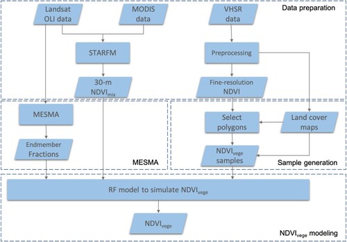
The framework comprised of four parts. First, the data were prepared. To prepare for the pair of 30-m NDVI images and NDVI_vege data extracted from VHSR, we generated a 30-m NDVI time series using STARFM and preprocessed VHSR images. The selected pair of 30-m NDVI images and VHSR images should be on the same date or close dates. Second, Multiple Endmember Spectral Mixture Analysis (MESMA). MESMA was applied to the 30-m NDVI image to derive fractions of endmembers within a pixel. The NDVI values of the non-vegetation endmembers were determined and assumed to be constant throughout the year. Third, we consider sample generation. For each VHSR image, a land cover map was created using the object-based classification method. We randomly selected sample pixels in the 30-m NDVI images and delineated the corresponding polygons on the VHSR images, within which the mean NDVI of vegetation was treated as the true NDVI_vege. Fourth, NDVI_vege modeling. The random forest (RF) regression model was trained with samples to estimate the NDVI_vege.

The framework to simulate subpixel NDVI_vege from pairs of a 30-m NDVI image and a VHSR image is summarized in Figure 1. Although the NDVI_vege product maintains a spatial resolution of 30 m, it represents the vegetation NDVI within a mixed pixel, rather than reflecting the composite NDVI value arising from the mixed constituents, as derived from the original reflectance imagery.

Figure 1. Flowchart of the framework. NDVI_mix represents 30-m spatial resolution NDVI data and NDVI_vege represents the subpixel vegetation NDVI.

2.2. Study area

The proposed framework was tested to derive the NDVI_vege time series for Wuhan (113°41’E–115°05’E, 29°50’N–31°22’N), a metropolis located in central China (Figure 2). Wuhan is the capital of the Hubei Province and covers an area of 8569.15 km². Wuhan’s climate is humid subtropical, with an annual total precipitation of 1315 mm and an annual mean temperature of 17.13°C. Wuhan has a wealth of water and forest resources, and contains 166 lakes and over 70 parks.

Figure 2. Study area and locations of VHSR satellite images used to calibrate and validate the framework.

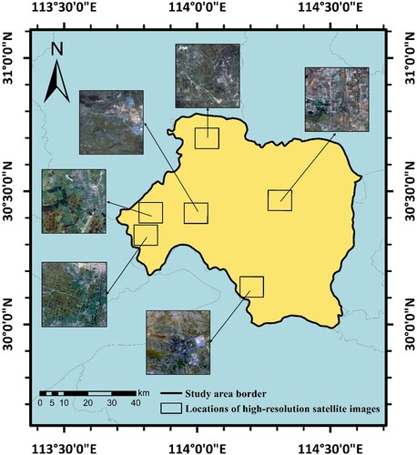
Wuhan has grown rapidly over the last three decades. The urban area in Wuhan increased from 658.64 km² in 1990 to 1362.77 km² in 2015 based on the remote sensing monitoring data (Li, Wang, and Song 2022), and the urban landscape becomes more fragmented. Our study area includes 11 out of 13 districts in Wuhan, which are within one tile of the Landsat images.

2.3. Datasets and processing

2.3.1. Satellite data

1. 30-m NDVI times series

Landsat OLI surface reflectance images (path 123 row 039, cloud cover < 20%) from 2013 and 2015 were downloaded from the US Geological Survey (USGS) Earth Resources Observation Systems (EROS) data center. To generate the 30-m NDVI time series, Landsat OLI images were fused with 8-day MODIS composites (MOD09A1, from the Terra platform) using STARFM. MOD09A1 images, which had a 500-m spatial resolution and seven spectral bands, were downloaded from the EOS data gateway of NASA’s Goddard Space Flight Center (https://earthexplorer.usgs.gov). Please refer to Gao et al. (2006) and our previous study (Liu et al. 2018) for details on data fusion.

(2)	VHSR satellite images

Six VHSR satellite images from WorldView-2 and Gaofen-2 (GF-2), which covered a part of the study area with a cloud cover of less than 10%, were used to extract NDVI_vege. WorldView-2 collects images at 0.5-m panchromatic (PAN) and 2-m multispectral (MS) bands. WorldView-2 images from March 4th, June 13th, and September 18th, 2013, were used in this study. GF-2 employs two PAN and MS cameras capable of collecting images with spatial resolutions of 1 and 4 m in the PAN and MS bands, respectively. Gaofen-2 images from April 22^nd, August 14th, and September 2nd, 2015, were downloaded from the China Centre for Resources Satellite Data and Application (http://www.cresda.com/CN/). Table 1 summarizes the band wavelengths and spatial resolutions of the VHSR satellite images used in the study. The VHSR images were orthorectified and projected onto a UTM_Zone_49N projection.

Table 1. The band wavelengths and the spatial resolution of VHSR satellite images used in this study.

GF-2			WorldView-2
Band order	Wavelengths (nm)	Spatial resolution (m)	Band order	Wavelengths (nm)	Spatial resolution (m)
Band 1	450–520	4	Band 2	450–510	2
Band 2	520–590	4	Band 3	510–580	2
Band 3	630–690	4	Band 4	585–625	2
Band 4	770–890	4	Band 7	770–895	2

2.3.2. Meteorological data

To estimate the vegetation GPP in the study area, we obtained daily meteorological data from 15 weather stations within and around the study area in 2013 and 2015. Meteorological data, including minimum temperature, relative humidity, and solar radiation, were downloaded from the Chinese National Meteorological Information Center (http://data.cma.gov.cn). The daily vapor pressure deficit (VPD) was calculated using the daily mean relative humidity (RH) and vapor pressure (VP) ($VPD=VP\times 100/RH-VP$).

Daily meteorological data were averaged every eight days and interpolated at 30-m spatial resolution using the inverse distance weighting method.

2.4. MESMA and accuracy assessment

Linear spectral mixture analysis assumes that the reflectance measurement of a mixed-composition pixel is a linear combination of the reflectance from endmembers (Powell et al. 2007). MESMA is a linear spectral mixture analysis that allows the number and type of endmembers to vary with the pixels. MESMA, including creating the spectral library, was conducted with VIPER Tool 2.1 (http://www.vipertools.org/), an add-on of ENVI (L3Harris Geospatial Solutions, Inc., Broomfield, U.S.) (Roberts, Halligan, and Philip 2007).

First, we manually extracted the spectra of the endmembers from each Landsat OLI image to build large reference libraries. According to the land cover types in the study area, endmembers selected from the images included grasslands, croplands, forests, rivers, lakes, and built-up areas. These endmembers were divided into spectrally distinct categories: vegetation, water bodies, and impervious surfaces. The reference endmember library was then reduced to 35 endmembers for the 2013 image and 33 endmembers for the 2015 image following the procedure outlined by Roth, Dennison, and Roberts (2012).

MESMA was applied to each image to estimate the endmember fractions. The default shade endmember in VIPER Tools was used in this study. According to previous studies, a maximum RMSE value of 2.5% and a threshold RMSE value of 0.7% were used to restrict MESMA (Roth et al. 2012; Wetherley, Roberts, and McFadden 2017). In addition, fractions of subpixel endmembers were constrained between 0 and 1, and no pixels contained shade endmembers higher than 80%. The maximum three-endmember combination was set in this study because previous studies have shown that model complexity is positively related to computing time and negatively related to accuracy (Powell et al. 2007). MESMA evaluates all possible endmember combinations pixel-by-pixel to select the best-fitting model. Fraction images from 2013 and 2015 are shown in Figures S1 and S2, respectively.

To assess the accuracy of the MESMA results, we randomly selected 60 pairs of samples generated as described in Section 2.6. Because this study focused on deriving NDVI_vege from mixed pixels, we compared the vegetation fractions of MESMA and those extracted from VHSR to validate the MESMA results (Figure S3).

2.5. Land cover classifications

For each VHSR image, an object-based classification method was used to classify the study area into vegetation, built-up areas, water bodies, and shade, corresponding to the endmember types in MESMA. The RGB image was first segmented into objects using the Trimble eCognition software (Trimble Inc., Sunnyvale, U.S.). The most commonly used method to choose segmentation parameters is visual inspection (Im et al. 2014). We manually experimented using multiple segmentation parameters. For the WorldView-2 images, we chose scale = 110, shape = 0.3, and compactness = 0.5; for the GF-2 images, we chose scale = 100, shape = 0.3, and compactness = 0.5. The support vector machine (SVM) algorithm was then applied to classify objects into different land cover types. Built-up areas, water bodies, and shade were treated as nonvegetated areas.

Moreover, 30-m land cover maps for 2013 and 2015 were created using Landsat OLI images to parameterize the GPP estimation model. Each pixel was identified as the land cover type with the maximum fraction from the unmixing result. Multi-season NDVI values and spectral reflectance of the base scenes (Landsat OLI images of September 10th, 2013 and September 8th, 2015) were used as inputs of an SVM model to classify vegetation into evergreen broadleaf forest (EBF), deciduous broadleaf forest (DBF), grassland, and cropland. This study ignored needle trees and shrubs, because needle trees and shrubs are not the dominant tree type in Wuhan, usually mixed with broadleaf trees.

To train and validate the supervised classification model, we collected samples for each image through visual interpretation of Landsat and VHRS images. We randomly selected 80% of the samples as the training dataset, and the remaining samples as the testing dataset for each image. Table S1 provides the overall accuracy of the classifications based on Landsat OLI, GF-2, and Worldview-2 images.

2.6. Sample generation

To estimate subpixel NDVI_vege using a machine learning model, we collected NDVI samples from pairs of Landsat OLI and VHSR images. Pixels in the Landsat OLI images with vegetation fractions higher than 70% were identified as pure pixels. We assumed that subpixel extraction of NDVI_vege was not necessary for these pure vegetation pixels. We also assumed that NDVI_vege from pixels with vegetation fractions lower than 10% can be ignored because minimal vegetation fractions may greatly bias the model to extract NDVI_vege. Pixels with vegetation fractions higher than 10% but lower than 70% were randomly selected for each Landsat OLI image. The polygon was composed of 15$\times$15 pixels for the WorldView-2 images and 8$\times$8 pixels for the Gaofen-2 images. The corresponding polygons were generated on the paired VHSR image. The land cover fraction within a polygon was computed as the ratio of the pixels of a certain land cover type to the total number of pixels. Land-cover fractions calculated based on VHSR were used to evaluate the performance of MESMA. The mean NDVI of the vegetation pixels within a polygon was treated as the true NDVI_vege. NDVI_mix from selected pixels in the Landsat OLI image and NDVI_vege from the corresponding polygons in the VHSR images were used to train and validate the machine learning model.

2.7. Predicting subpixel NDVI_vege

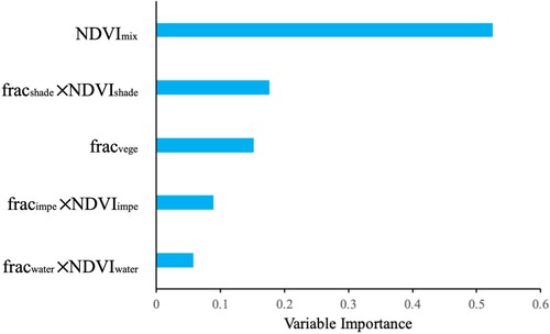
The NDVI_vege within a 30-m pixel was derived using the RF regression algorithm. RF is a nonlinear ensemble learning method for classification or regression purposes through constructing and averaging a large number of randomized decision trees (Hastie, Tibshirani, and Friedman 2009). The advantage of the RF algorithm is its suitability for a small sample size and the quantitative assessment of the contribution of individual predictors (Hastie, Tibshirani, and Friedman 2009; Hutengs and Vohland 2016). As presented in Equation (1), the inputs of the RF model include NDVI_mix, the fraction of the vegetation endmember, and the product of the fractions of impervious surface, water, and shade endmembers and their NDVI values. For simplicity, the NDVI of a non-vegetated land cover type was calculated as the average NDVI value of reference endmembers with the same land cover type. The variable importance score was used to evaluate the contributions of the input features in predicting the NDVI_vege.

In this study, we specified two parameters in the RF regression model: the number of variables selected at each split (mtry), and the overall number of trees (ntree) that are grown. The ntree value was evaluated from 100 to 1000 at intervals of 100, and was determined once the out-of-bag error stabilized. The mtry value was evaluated to be approximately one-third of the number of input features until a minimal out-of-bag error of prediction was achieved. Two-thirds of the samples were randomly selected to train the RF model, and the remaining samples were used to validate the regression model. The RF regression model was implemented using Python3.5, with the scikit-learn 0.19.1.

Considering the seasonal variations in NDVI and the availability of VHSR images, we built two RF regression models each year, with one for the meteorological spring and summer (from March to August) and the other for fall and winter (from September to February). The R² and root mean square error (RMSE) were used to evaluate the differences between the estimated subpixel NDVI_vege and true NDVI_vege derived from VHSR images. Samples from the WorldView-2 image of March 4th and June 13th, 2013, and from the Gaofen-2 image on April 22^nd and August 14th, 2015, were used to train the spring and summer model. Samples generated from September VHSR images were used to train and validate the fall and winter models.

To test the hypothesis that the RF-based nonlinear model outperforms the linear unmixing method in extracting the subpixel NDVI_vege in urban areas, we compared the results from the proposed framework to those derived from the linear unmixing method, using the same validation dataset. The least square linear regression model was employed to solve the endmember NDVI with a 5$\times$5-pixel window, assuming that the NDVI of endmembers was constant across these pixels. Details of the linear unmixing method can be found in Atzberger et al. (2014).

2.8. GPP estimation

In this study, GPP was estimated using the MOD17 algorithm, a light-use efficiency (LUE)-based method (Monteith 1972). GPP was calculated as (Running et al. 2000): (3) $GPP(kgC{m}^{-2}da{y}^{-1})=\epsilon (kgCM{J}^{-1})\times fPAR\times PAR(MJ{m}^{-2}da{y}^{-1})$(3) where fPAR is the fraction of the amount of photosynthetically active radiation (PAR) absorbed by the canopy and Ɛ is a maximum light use efficiency term. The fPAR was computed with NDVI_mix and NDVI_vege separately using the equation proposed by Myneni and Williams (1994): (4) $fPAR=1.1638NDVI-0.1426$(4)

The value of Ɛ was calculated as: (5) $\epsilon =LUE(kgCM{J}^{-1})\times T_{MIN}scalar\times VPDscalar$(5) where LUE is the maximum light-use efficiency parameter, T_MIN is the daily minimum air temperature, and VPD is the daytime VPD. Please refer to Zhao and Running (2010) for details on calculating the T_MIN and VPD scalars.

The LUE was assumed constant for each type of vegetation. The LUE values were obtained from the modified Biome-Property-Look-Up-Table (BPLUT) provided by Zhao and Running (Zhao and Running 2010). To determine the LUE value for the pixels that were not classified as vegetation but with a vegetation cover higher than 1, a 5$\times$5-pixel window was used to search for surrounding vegetation pixels and assign the vegetation type of the first vegetation pixel as the subpixel vegetation type to be determined. If there were no surrounding vegetation pixels, the GPP would not be calculated.

GPP estimated with NDVI_vege was compared with GPP estimated with NDVI_mix to illustrate the uncertainty in GPP estimations. These uncertainties may arise from the extensive presence of mixed pixels in urban areas.

3. Results

3.1. Performance of the framework

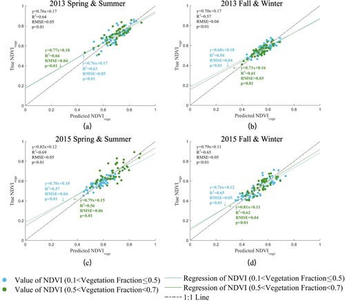
Figures 3 and 4 illustrate the goodness of fit of the true NDVI_vege and NDVI_vege predicted by the proposed framework and linear unmixing method, respectively. Overall, the proposed framework provided more accurate NDVI_vege predictions than the linear unmixing method, with lower RMSE and higher R² values. The accuracy of the predicted NDVI_vege varied slightly with season for both models. The predictions for spring and summer were less accurate than those for fall and winter were. In the spring and summer seasons, when the NDVI changed rapidly, the proposed framework outperformed the linear unmixing model.

Figure 3. Comparison of NDVI_vege derived from the proposed framework and the true NDVI_vege extracted from the VHSR images for the spring & summer seasons of 2013 (a), fall & winter seasons of 2013 (b), spring & summer seasons of 2015 (c), and fall & winter seasons of 2015 (d).

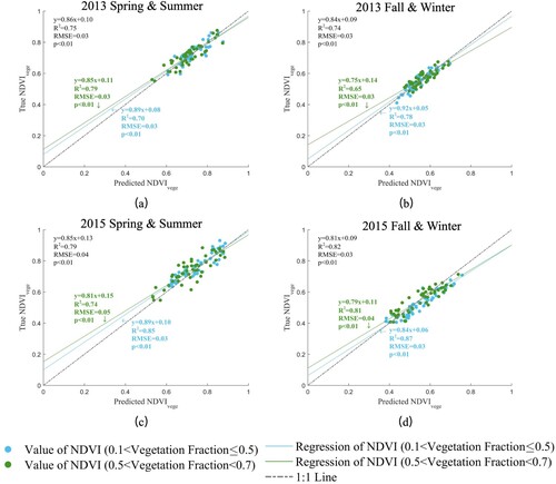
Figure 4. Comparison of NDVI_vege derived from the linear unmixing model and the true NDVI_vege extracted from the VHSR images for the spring & summer seasons of 2013 (a), fall & winter seasons of 2013 (b), spring & summer seasons of 2015 (c), and fall & winter seasons of 2015 (d).

To analyze the impacts of vegetation fraction on predicting NDVI_vege, we evaluated the prediction accuracy for low vegetation cover (0.1$<$vegetation fraction $\le 0.5$) and high vegetation cover (0.5$<$vegetation fraction$<$0.7). For the proposed framework, the NDVI_vege estimates corresponding to regions with low vegetation cover demonstrated slightly superior accuracy compared to those with high vegetation cover in the fall and winter seasons of 2013 and throughout all seasons of 2015. However, for the linear unmixing model, the impact of vegetation fraction on the estimation accuracy was not noticeable. Because the proposed nonlinear framework yielded more accurate estimations of NDVI_vege, the following analyses were conducted on the results of the proposed framework.

The variable importance score derived from the RF regression model demonstrated that NDVI_mix was the most important predictor of NDVI_vege (Figure 5). Following NDVI_mix, $fra{c}_{shade}\times NDV{I}_{shade}$ and $fra{c}_{vege}$ were equally important predictors of NDVI_vege.

Figure 5. Variable importance score of the input features of the RF regression model to predict NDVI_vege.

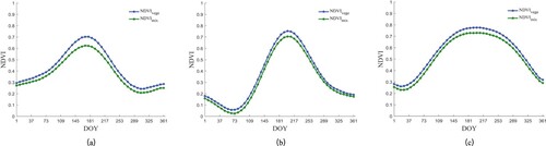
The proposed nonlinear framework was then applied to generate an 8-day NDVI_vege time series for an entire year. The NDVI_vege time series was compared with the NDVI_mix time series for pixels with different vegetation fractions. Figure 6 illustrates that NDVI_vege is generally higher than NDVI_mix. The difference between NDVI_vege and NDVI_mix was more pronounced from June to August, when the NDVI reached its maximum. The difference between NDVI_vege and NDVI_mix was greater in pixels with a lower vegetation fraction than in those with a higher vegetation fraction.

Figure 6. Examples of NDVI_vege and NDVI_mix time series for pixels with the vegetation fraction of 20% (a), 40% (b), and 60% (c).

3.2. Estimation of GPP with NDVI_vege

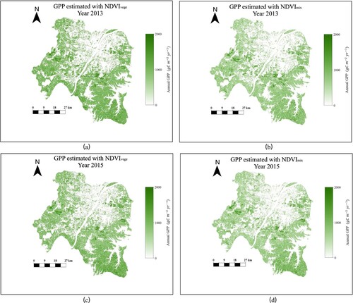
Figure 7 shows the spatial distribution of GPP estimated using NDVI_vege and NDVI_mix. GPP estimated with NDVI_vege was generally higher than GPP estimated using NDVI_mix. The differences between the GPP estimated with NDVI_vege and those estimated with NDVI_mix were mainly located in the suburban area, where cropland and wood coexisted with houses, roads, and ponds. Differences can also be found in metropolitan areas where parks and green belts are intermingled with built-up areas.

Figure 7. Map of the annual GPP estimated with NDVI_vege ((a) and (c)) and NDVI_mix ((b) and (d)), respectively.

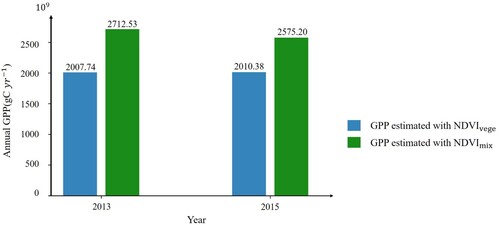
The total annual GPP estimated with NDVI_vege in the study area was calculated and compared with that estimated using NDVI_mix. Figure 8 illustrates that the total annual GPP estimated with NDVI_vege was 35% and 28% higher than the total annual GPP estimated with NDVI_mix in 2013 and 2015, respectively.

Figure 8. Comparison between the annual total GPP estimated with NDVI_vege and the annual total GPP estimated with NDVI_mix.

4. Discussion

Evaluating vegetation productivity dynamics in urban areas using remotely sensed images gains particular significance in the context of larger and rapidly expanding cities, as vegetation has been frequently degraded or removed in the process of urbanization (Liu and Yang 2013). Although the Landsat series and Sentinel-2 provide valuable medium-spatial-resolution image resources, landscapes in urban areas are highly mixed, even in the 10-30 m pixel, considering that the general rule for the minimum pixel size is half the size of the smallest object of interest (Myint et al. 2011; Song 2005). Therefore, this study developed a novel framework to extract the subpixel NDVI of vegetation endmembers using NDVI_mix, endmember fractions, non-vegetation endmember NDVI, and the RF algorithm. This framework is useful for addressing the mixed pixel problem in estimating the vegetation primary productivity in urban areas.

4.1. Advantages over the linear unmixing method and spatial-temporal fusion algorithm

In this study, a comparison analysis showed that the proposed nonlinear framework provided more accurate predictions of NDVI_vege than the linear unmixing method. However, the difference between these two methods was more than whether the relationship between the NDVI_mix and NDVI of the endmembers was nonlinear. The linear unmixing method was employed in a region to provide a number of functions to solve the NDVI values of several endmembers, assuming that intra-class variations within the region can be neglected. This was possibly true for non-vegetated surfaces, but the vegetation NDVI may vary within the region of heterogeneous urban areas (Neyns and Canters 2022). The size of the selected region may influence the accuracy of NDVI_vege (Atzberger et al. 2014), whereas the proposed nonlinear framework is free of this issue.

Unlike the spatiotemporal fusion algorithm, which requires pairs of coarse- and fine-resolution images of the entire area to establish a pixel-by-pixel relationship (Gao et al. 2006; Gärtner, Förster, and Kleinschmit 2016; Zhu et al. 2016; Zurita-Milla, Clevers, and Schaepman 2008), the proposed framework estimated NDVI_vege based on the general nonlinear relationship between NDVI_vege and endmember fractions, endmember NDVI, and NDVI_mix in the study area. Thus, VHSR did not cover the entire study area. VHSR images of small areas distributed in a city can provide ground truths of NDVI_vege, which were used to train the RF regression model to extract NDVI_vege. The product maintained a spatial resolution of 30 m, but NDVI_vege represented the value of the vegetation endmember within a mixed pixel. The spatiotemporal fusion method has rarely been applied to a blend of medium-resolution images and VHSR, owing to the high cost and limited spatial–temporal coverage of VHSR data (Gärtner, Förster, and Kleinschmit 2016). The proposed framework provides a cost-effective approach for resolving the subpixel NDVI from complex mixed pixels in urban areas.

4.2. Accuracy of NDVI_vege

The proposed framework provided accurate NDVI_vege estimations for mixed pixels, regardless of vegetation fraction and season. For pixels with a low vegetation fraction, NDVI_mix was reduced by the non-vegetation endmembers, particularly during the mid-growing season of vegetation. Therefore, the differences between NDVI_vege and NDVI_mix were more pronounced than those in pixels with a high vegetation fraction. Accurate estimation of endmember fractions is important for estimating the NDVI_vege. However, many factors, such as illumination effects and similar spectra of different endmembers, can cause uncertainty in the MESMA results (Roth, Dennison, and Roberts 2012; Wetherley, Roberts, and McFadden 2017), which could further influence the accuracy of NDVI_vege estimations. Nevertheless, it is important to note that NDVI_vege was only an approximation of the vegetation endmember within a mixed pixel, given the combinations of different endmembers estimated by MESMA.

To generate the NDVI_vege time series for GPP estimation, medium-spatial-resolution NDVI time series are required. In this study, STARFM was used to generate 30-m and 8-day NDVI_mix time series as an intermediate step. To account for the seasonal change in NDVI_vege, we built a regression model for the spring, summer, fall, and winter seasons separately. However, the accuracy of NDVI_vege simulations did not vary with seasons, possibly because the accuracy of NDVI_vege simulations depended on the quality of the NDVI_mix time series, which was the base data for the temporal analysis. The proposed framework adjusts the NDVI value on top of NDVI_mix while preserving the seasonal trend of NDVI_mix. Further studies are needed to evaluate the impact of the number of VHSR used in the framework to simulate seasonal NDVI_vege.

4.3. Implications to GPP estimations

Mixed pixels in urban areas affect the GPP estimation in two ways. First, the mixture of vegetated and non-vegetated surfaces in a pixel affects the accurate estimation of fPAR. Second, when multiple plant functional types exist in one pixel, the unique plant-type label affects the accurate estimation of the fPAR. Although the mixed pixel effect has been acknowledged in the literature, this is one of the first studies to examine subpixel vegetation GPP in urban areas. The difference between the GPP estimated with NDVI_vege and the GPP estimated NDVI_mix implied uncertainty in the GPP estimation, which was mainly caused by the mixed pixels of vegetated and non-vegetated surfaces. NDVI_mix may underestimate GPP by 28-35%, because fPAR could be underestimated by the reduced NDVI values when vegetation was mixed with impervious surface, bare soil, shade, or water. In addition, vegetation in the pixels with low vegetation fractions (frac_vege< 50%) could be ignored when calculating GPP with NDVI_mix, since such 30-m pixels would not be identified as vegetation.

This framework has two limitations in the estimation of GPP. First, the framework cannot identify plant functional types within a pixel, particularly if more than one plant functional type exists in a pixel. It was difficult to determine the subpixel vegetation type if there were no vegetation pixels (frac_vege> = 50) in the neighborhood. Therefore, GPP estimated with NDVI_vege may miss small areas of vegetation surrounded by built-up surfaces in metropolitan areas. The time series of VHSR images remains the optimal solution for accurately estimating the GPP in urban areas. Before VHSR images become more feasible and cost-friendly, the framework proposed in this study provides a novel and efficient approach to accurately extract subpixel NDVI values and quantify vegetation primary productivity in heterogeneous urban areas.

Second, GPP was estimated with one form of the LUE model in the framework. In the last two decades, the original LUE model was improved in the descriptions of environmental stresses regulations on GPP (Xiao et al. 2011), the relationship between vegetation index and fPAR (Zhang et al. 2014), parameterization schemes (Zheng et al. 2018), and the choice of vegetation index (Middleton et al. 2016). Different models can result in marked discrepancies in GPP estimates (Zheng et al. 2018), which will affect the assessment of the uncertainty in GPP estimations caused by mixed pixels. In addition to LUE model, ecosystem process model has also been widely used to estimate GPP at large scale (Xiao et al. 2019). However, to our knowledge, the mixed pixel effect has not been studied for ecosystem process model. Thus, further studies are needed to thoroughly evaluate the mixed pixel effect on the GPP estimation based on multiple GPP models.

5. Conclusions

We proposed an RF-based framework to extract subpixel NDVI_vege from mixed pixels in urban areas using NDVI_mix, endmember fractions, and the average NDVI of non-vegetation endmembers. Results demonstrated that the NDVI_vege extracted by this framework agreed well with the true NDVI_vege cross seasons and vegetation fractions, with R² ranging from 0.74 to 0.82 and RMSE ranging from 0.03 to 0.04. The framework was then applied to generate the NDVI_vege time series to estimate the GPP in the study area. The total annual GPP estimated with NDVI_vege was 28%-35% higher than the total annual GPP estimated with NDVI_mix, indicating the uncertainty in the GPP estimations caused by the mixed pixels. The proposed framework for simulating NDVI_vege will be of great interest for monitoring vegetation dynamics (e.g. fPAR, leaf area index, or vegetation greenness) in heterogeneous areas.

Disclosure statement

No potential conflict of interest was reported by the author(s).

Data availability statement

Data that support the findings of this study can be obtained from the corresponding author upon reasonable request.

Additional information

Funding

This research was supported by the National Key Research and Development Program of China (No. 2022YFB3903405), National Natural Science Foundation of China (General Program: 42171466 and 42171350), and and the Fundamental Research Funds for the Central Universities (2662021JC002).

References

- Asner, G. P., C. A. Wessman, and J. L. Privette. 1997. “Unmixing the Directional Reflectances of AVHRR Sub-Pixel Landcovers.” IEEE Transactions on Geoscience and Remote Sensing 35 (4): 868–878. https://doi.org/10.1109/36.602529.
- Atzberger, C., A. R. Formaggio, Y. E. Shimabukuro, T. Udelhoven, M. Mattiuzzi, G. A. Sanchez, and E. Arai. 2014. “Obtaining Crop-Specific Time Profiles of NDVI: The Use of Unmixing Approaches for Serving the Continuity between SPOT-VGT and PROBA-V Time Series.” International Journal of Remote Sensing 35 (7): 2615–2638. https://doi.org/10.1080/01431161.2014.883106.
- Busetto, L., M. Meroni, and R. Colombo. 2008. “Combining Medium and Coarse Spatial Resolution Satellite Data to Improve the Estimation of Sub-Pixel NDVI Time Series.” Remote Sensing of Environment 112 (1): 118–131. https://doi.org/10.1016/j.rse.2007.04.004.
- Chen, J. M., X. Chen, and W. Ju. 2013. “Effects of Vegetation Heterogeneity and Surface Topography on Spatial Scaling of Net Primary Productivity.” Biogeosciences 10 (7): 4879–4896. https://doi.org/10.5194/bg-10-4879-2013.
- Chen, Xiang, Dawei Wang, Jin Chen, Cong Wang, and Miaogen Shen. 2018. “The Mixed Pixel Effect in Land Surface Phenology: A Simulation Study.” Remote Sensing of Environment 211 (June): 338–344. https://doi.org/10.1016/j.rse.2018.04.030.
- Churkina, G. 2008. “Modeling the Carbon Cycle of Urban Systems.” Ecological Modelling 216 (2): 107–113. https://doi.org/10.1016/j.ecolmodel.2008.03.006
- Gao, Feng, J. Masek, M. Schwaller, and F. Hall. 2006. “On the Blending of the Landsat and MODIS Surface Reflectance: Predicting Daily Landsat Surface Reflectance.” IEEE Transactions on Geoscience and Remote Sensing 44 (8): 2207–2218. https://doi.org/10.1109/TGRS.2006.872081.
- Gärtner, Philipp, Michael Förster, and Birgit Kleinschmit. 2016. “The Benefit of Synthetically Generated RapidEye and Landsat 8 Data Fusion Time Series for Riparian Forest Disturbance Monitoring.” Remote Sensing of Environment 177 (May): 237–247. https://doi.org/10.1016/j.rse.2016.01.028.
- Hastie, Trevor, Robert Tibshirani, and Jerome Friedman. 2009. “Random Forests.” In The Elements of Statistical Learning, edited by Trevor Hastie, Robert Tibshirani, and Jerome Friedman, 587–604. Springer Series in Statistics. New York, NY: Springer New York. https://doi.org/10.1007/978-0-387-84858-7_15.
- Hilker, T., M. A. Wulder, N. C. Coops, J. Linke, G. McDermid, J. G. Masek, F. Gao, and J. C. White. 2009. “A New Data Fusion Model for High Resolution Mapping of Forest Disturbance Based on Landsat and MODIS.” Remote Sensing of Environment 113 (8): 1613–1627. https://doi.org/10.1016/j.rse.2009.03.007
- Hu, Z., S. Piao, A. K. Knapp, X. Wang, S. Peng, W. Yuan, S. Running, et al. 2022. “Decoupling of Greenness and Gross Primary Productivity as Aridity Decreases.” Remote Sensing of Environment 279 (September): 113120. https://doi.org/10.1016/j.rse.2022.113120.
- Hutengs, Christopher, and Michael Vohland. 2016. “Downscaling Land Surface Temperatures at Regional Scales with Random Forest Regression.” Remote Sensing of Environment 178 (June): 127–141. https://doi.org/10.1016/j.rse.2016.03.006.
- Im, Jungho, Lindi J. Quackenbush, Manqi Li, and Fang Fang. 2014. “Optimum Scale in Object-Based Image Analysis.” In Scale Issues in Remote Sensing, edited by Qihao Weng, 197–214. Hoboken, New Jersey: John Wiley & Sons, Inc. https://doi.org/10.1002/9781118801628.ch10.
- Imhoff, M. L., L. Bounoua, R. DeFries, W. T. Lawrence, D. Stutzer, C. J. Tucker, and T. Ricketts. 2004. “The Consequences of Urban Land Transformation on Net Primary Productivity in the United States.” Remote Sensing of Environment 89 (4): 434–443. https://doi.org/10.1016/j.rse.2003.10.015
- Li, Xiangmei, Ying Wang, and Yan Song. 2022. “Unraveling Land System Vulnerability to Rapid Urbanization: An Indicator-Based Vulnerability Assessment for Wuhan, China.” Environmental Research 211 (August): 112981. https://doi.org/10.1016/j.envres.2022.112981.
- Liu, Shishi, Wei Du, Hang Su, Shanqin Wang, and Qingfeng Guan. 2018. “Quantifying Impacts of Land-Use/Cover Change on Urban Vegetation Gross Primary Production: A Case Study of Wuhan, China.” Sustainability 10 (3): 714. https://doi.org/10.3390/su10030714.
- Liu, X., F. Pei, Y. Wen, X. Li, S. Wang, C. Wu, Y. Cai, et al. 2019. “Global Urban Expansion Offsets Climate-Driven Increases in Terrestrial Net Primary Productivity.” Nature Communications 10 (1): 5558. https://doi.org/10.1038/s41467-019-13462-1.
- Liu, Ting, and Xiaojun Yang. 2013. “Mapping Vegetation in an Urban Area with Stratified Classification and Multiple Endmember Spectral Mixture Analysis.” Remote Sensing of Environment 133 (June): 251–264. https://doi.org/10.1016/j.rse.2013.02.020.
- Middleton, E. M., K. F. Huemmrich, D. R. Landis, T. A. Black, A. G. Barr, and J. H. McCaughey. 2016. “Photosynthetic Efficiency of Northern Forest Ecosystems Using a MODIS-Derived Photochemical Reflectance Index (PRI).” Remote Sensing of Environment 187 (December): 345–366. https://doi.org/10.1016/j.rse.2016.10.021.
- Miller, David L., Dar A. Roberts, Keith C. Clarke, Yang Lin, Olaf Menzer, Emily B. Peters, and Joseph P. McFadden. 2018. “Gross Primary Productivity of a Large Metropolitan Region in Midsummer Using High Spatial Resolution Satellite Imagery.” Urban Ecosystems 21 (5): 831–850. https://doi.org/10.1007/s11252-018-0769-3.
- Monteith, J. L. 1972. “Solar Radiation and Productivity in Tropical Ecosystems.” Journal of Applied Ecology 9 (3): 747–766. https://doi.org/10.2307/2401901
- Myint, Soe W., Patricia Gober, Anthony Brazel, Susanne Grossman-Clarke, and Qihao Weng. 2011. “Per-Pixel vs. Object-Based Classification of Urban Land Cover Extraction Using High Spatial Resolution Imagery.” Remote Sensing of Environment 115 (5): 1145–1161. https://doi.org/10.1016/j.rse.2010.12.017.
- Myneni, R. B., and D. L. Williams. 1994. “On the relationship between FAPAR and NDVI.” Remote Sensing of Environment 49 (3): 200–211.
- Neyns, Robbe, and Frank Canters. 2022. “Mapping of Urban Vegetation with High-Resolution Remote Sensing: A Review.” Remote Sensing 14 (4): 1031. https://doi.org/10.3390/rs14041031.
- Nightingale, J. M., N. C. Coops, R. H. Waring, and W. W. Hargrove. 2007. “Comparison of MODIS Gross Primary Production Estimates for Forests across the U.S.A. with Those Generated by a Simple Process Model, 3-PGS.” Remote Sensing of Environment 109 (4): 500–509. https://doi.org/10.1016/j.rse.2007.02.004.
- Parazoo, Nicholas C., Red Willow Coleman, Vineet Yadav, E. Natasha Stavros, Glynn Hulley, and Lucy Hutyra. 2022. “Diverse Biosphere Influence on Carbon and Heat in Mixed Urban Mediterranean Landscape Revealed by High Resolution Thermal and Optical Remote Sensing.” Science of The Total Environment 806 (February): 151335. https://doi.org/10.1016/j.scitotenv.2021.151335.
- Powell, R., D. Roberts, P. Dennison, and L. Hess. 2007. “Sub-Pixel Mapping of Urban Land Cover Using Multiple Endmember Spectral Mixture Analysis: Manaus, Brazil.” Remote Sensing of Environment 106 (2): 253–267. https://doi.org/10.1016/j.rse.2006.09.005.
- Roberts, D. A. 2002. “Large Area Mapping of Land-Cover Change in Rondônia Using Multitemporal Spectral Mixture Analysis and Decision Tree Classifiers.” Journal of Geophysical Research 107 (D20): 8073. https://doi.org/10.1029/2001JD000374.
- Roberts, Dar, Kerry Halligan, and Dennison Philip. 2007. “VIPER Tools User Manual.” University of California Santa Barbara, Department of Geography.
- Roth, Keely L., Philip E. Dennison, and Dar A. Roberts. 2012. “Comparing Endmember Selection Techniques for Accurate Mapping of Plant Species and Land Cover Using Imaging Spectrometer Data.” Remote Sensing of Environment 127 (December): 139–152. https://doi.org/10.1016/j.rse.2012.08.030.
- Running, Steven W., Peter E. Thornton, Ramakrishna Nemani, and Joseph M. Glassy. 2000. “Global Terrestrial Gross and Net Primary Productivity from the Earth Observing System.” In Methods in Ecosystem Science, edited by Osvaldo E. Sala, Robert B. Jackson, Harold A. Mooney, and Robert W. Howarth, 44–57. New York, NY: Springer New York. https://doi.org/10.1007/978-1-4612-1224-9_4.
- Singh, Devendra. 2011. “Generation and Evaluation of Gross Primary Productivity Using Landsat Data Through Blending with MODIS Data.” International Journal of Applied Earth Observation and Geoinformation 13 (1): 59–69. https://doi.org/10.1016/j.jag.2010.06.007.
- Song, Conghe. 2005. “Spectral Mixture Analysis for Subpixel Vegetation Fractions in the Urban Environment: How to Incorporate Endmember Variability?” Remote Sensing of Environment 95 (2): 248–263. https://doi.org/10.1016/j.rse.2005.01.002.
- Wetherley, Erin B., Dar A. Roberts, and Joseph P. McFadden. 2017. “Mapping Spectrally Similar Urban Materials at Sub-Pixel Scales.” Remote Sensing of Environment 195 (June): 170–183. https://doi.org/10.1016/j.rse.2017.04.013.
- Xiao, J., F. Chevallier, C. Gomez, L. Guanter, J. A. Hicke, A. R. Huete, K. Ichii, et al. 2019. “Remote Sensing of the Terrestrial Carbon Cycle: A Review of Advances over 50 Years.” Remote Sensing of Environment 233 (November): 111383. https://doi.org/10.1016/j.rse.2019.111383.
- Xiao, Jingfeng, Kenneth J. Davis, Nathan M. Urban, Klaus Keller, and Nicanor Z. Saliendra. 2011. “Upscaling Carbon Fluxes from Towers to the Regional Scale: Influence of Parameter Variability and Land Cover Representation on Regional Flux Estimates.” Journal of Geophysical Research 116 (G3): G03027. https://doi.org/10.1029/2010JG001568.
- Zhang, Qingyuan, Yen-Ben Cheng, Alexei I. Lyapustin, Yujie Wang, Feng Gao, Andrew Suyker, Shashi Verma, and Elizabeth M. Middleton. 2014. “Estimation of Crop Gross Primary Production (GPP): FAPARchl Versus MOD15A2 FPAR.” Remote Sensing of Environment 153 (October): 1–6. https://doi.org/10.1016/j.rse.2014.07.012.
- Zhao, M., and S. W. Running. 2010. “Drought-Induced Reduction in Global Terrestrial Net Primary Production from 2000 Through 2009.” Science 329 (5994): 940–943. https://doi.org/10.1126/science.1192666.
- Zheng, Yi, Li Zhang, Jingfeng Xiao, Wenping Yuan, Min Yan, Tong Li, and Zhiqiang Zhang. 2018. “Sources of Uncertainty in Gross Primary Productivity Simulated by Light Use Efficiency Models: Model Structure, Parameters, Input Data, and Spatial Resolution.” Agricultural and Forest Meteorology 263 (December): 242–257. https://doi.org/10.1016/j.agrformet.2018.08.003.
- Zhong, Qiaoyan, Jun Ma, Bin Zhao, Xinxin Wang, Jiamin Zong, and Xiangming Xiao. 2019. “Assessing Spatial-Temporal Dynamics of Urban Expansion, Vegetation Greenness and Photosynthesis in Megacity Shanghai, China during 2000–2016.” Remote Sensing of Environment 233 (November): 111374. https://doi.org/10.1016/j.rse.2019.111374.
- Zhou, Junxiong, Jin Chen, Xuehong Chen, Xiaolin Zhu, Yuean Qiu, Huihui Song, Yunhan Rao, Chishan Zhang, Xin Cao, and Xihong Cui. 2021. “Sensitivity of Six Typical Spatiotemporal Fusion Methods to Different Influential Factors: A Comparative Study for a Normalized Difference Vegetation Index Time Series Reconstruction.” Remote Sensing of Environment 252 (January): 112130. https://doi.org/10.1016/j.rse.2020.112130.
- Zhu, Xiaolin, Fangyi Cai, Jiaqi Tian, and Trecia Williams. 2018. “Spatiotemporal Fusion of Multisource Remote Sensing Data: Literature Survey, Taxonomy, Principles, Applications, and Future Directions.” Remote Sensing 10 (4): 527. https://doi.org/10.3390/rs10040527.
- Zhu, X., J. Chen, F. Gao, X. Chen, and J. G. Masek. 2010. “An enhanced spatial and temporal adaptive reflectance fusion model for complex heterogeneous regions.” Remote Sensing of Environment 114 (11): 2610–2623. https://doi.org/10.1016/j.rse.2010.05.032.
- Zhu, Xiaolin, Eileen H. Helmer, Feng Gao, Desheng Liu, Jin Chen, and Michael A. Lefsky. 2016. “A Flexible Spatiotemporal Method for Fusing Satellite Images with Different Resolutions.” Remote Sensing of Environment 172 (January): 165–177. https://doi.org/10.1016/j.rse.2015.11.016.
- Zurita-Milla, R., J. Clevers, and M. E. Schaepman. 2008. “Unmixing-Based Landsat TM and MERIS FR Data Fusion.” IEEE Geoscience and Remote Sensing Letters 5 (3): 453–457. https://doi.org/10.1109/LGRS.2008.919685.