Modeling landslide susceptibility based on convolutional neural network coupling with metaheuristic optimization algorithms

ABSTRACT

Landslides are one of the most common geological hazards worldwide, especially in Sichuan Province (Southwest China). The current study's main purposes are to explore the potential applications of convolutional neural networks (CNN) hybrid ensemble metaheuristic optimization algorithms, namely beluga whale optimization (BWO) and coati optimization algorithm (COA), for landslide susceptibility mapping in Sichuan Province (China). For this aim, fourteen landslide conditioning factors were compiled in a spatial database. The effectiveness of the conditioning factors in the development of the landslide predictive model was quantified using the linear support vector machine model. The receiver operating characteristic (ROC) curve (AUC), the root mean square error, and six statistical indices were used to test and compare the three resultant models. For the training dataset, the AUC values of the CNN-COA, CNN-BWO and CNN models were 0.946, 0.937 and 0.855, respectively. In terms of the validation dataset, the CNN-COA model exhibited a higher AUC value of 0.919, while the AUC values of the CNN-BWO and CNN models were 0.906 and 0.805, respectively. The results indicate that the CNN-COA model, followed by the CNN-BWO model, and the CNN model, offers the best overall performance for landslide susceptibility analysis.

KEYWORDS:

• Landslide susceptibility; convolutional neural network; beluga whale optimization; coati optimization algorithm; hybrid models
• Sichuan Province

1. Introduction

Landslides are considered to be one of the most harmful environmental hazards in mountainous areas, causing heavy losses to human life and infrastructure projects every year (Schuster 1996; GAR 2009; 2019; Ghorbanzadeh, Gholamnia, and Ghamisi 2022; Trinh et al. 2022; Yang et al. 2023). Official statistics show that from 2010 to 2019, there were approximately 90,000 landslide events in China, resulting in about 8,000 fatalities and tens of billions of dollars in economic losses (Lv et al. 2022). Sichuan Province experiences 25% of all geohazards in China annually, and landslides account for 69% of these events. Landslide occurrences are largely affected by various factors, including geoenvironmental factors (e.g. topography, tectonics, land use, etc.) and triggering factors (rainfall, earthquakes, glacier outburst, etc.) (Carrara et al. 1991; Petley 2012; Okalp and Akgün 2016; Okalp and Akgün 2022; Merghadi et al. 2020). Therefore, landslide susceptibility mapping (LSM), defined as the possibility of a landslide occurrence under a specific set of conditioning factors, is strongly recommended as a crucial step for disaster prevention and mitigation (Brabb 1984). Local governments can make more informed land use and development decisions for landslide-prone regions with the help of LSM. However, new techniques with strong prediction capabilities still need to be used to increase the accuracy of LSM.

Commonly used landslide susceptibility models can be grouped into four main types: heuristic, deterministic, statistical, and machine learning models (Merghadi et al. 2020). Heuristic models, such as the analytic hierarchy process (Abedini and Tulabi 2018; Azarafza, Ghazifard, and Asghari-Kaljahi 2018) and weighted linear combination (Hung et al. 2016), primarily rely on the subjective judgments of relevant experts. The model is time-efficient and can be applied at any size of study (Guzzetti et al. 1999). The major shortcoming of heuristic models is their subjectivity, which is related to the expert knowledge-based experiential assessment of landslide preparatory factors. Deterministic models use simplified, physically-based landslide modeling techniques to analyze slope instability (Ji et al. 2022). By explicitly or implicitly utilizing numerical models to predict a scenario resulting from the understanding of the effect of assigned elements on slope stability, deterministic models solve the difficulty of studying and predicting hazards (Mebrahtu et al. 2022; Wei et al. 2023). These models can produce precise results and provide a good depth of study of landslide mechanisms. Deterministic models, however, require significant amounts of detailed data to provide credible results for large-scale studies (i.e. at the watershed level up to the county/provincial level), which comes at a high cost both financially and computationally (Youssef and Pourghasemi 2021). Therefore, deterministic models are currently not applicable for large area susceptibility zonation exercises. Statistical models were created to investigate relationships between contributing factors and the occurrence of landslides due to the difficulties of applying deterministic models (Reichenbach et al. 2018). Different types of statistical models, such as the frequency ratio (FR) (Berhane, Kebede, and Alfarrah 2021), logistic regression (Eker et al. 2015; Zhao and Chen 2023), Dempster-Shafer theory (Shirani, Pasandi, and Arabameri 2018), weight of evidence (Ozturk and Uzel-Gunini 2022), and entropy index (Hodasová and Bednarik 2021), have been used to map landslide susceptibility. When predicting the spatial distribution of landslides, statistical models offer a more flexible and cost-effective method (Huang et al. 2021). It should be noted, however, that statistical models perform poorly in assessing the nonlinear relationship between the occurrence of landslides and conditioning factors. To overcome the limitations of statistical models, machine learning models have been introduced for LSM. Various machine learning models have been employed in LSM such as support vector machines (Dou et al. 2020), artificial neuronal networks (Eker et al. 2012; Lucchese, de Oliveira, and Pedrollo 2021), decision tree (Guo et al. 2021), random forest (Taalab, Cheng, and Zhang 2018; Sun et al. 2021), naïve bayes (Youssef and Pourghasemi 2021), classification and regression tree (Pourghasemi and Rahmati 2018), and maximum entropy (Kornejady, Ownegh, and Bahremand 2017). Machine learning models are highly suggested due to their ability to address nonlinear real-world problems (Hu et al. 2020). However, classical machine learning models may find erroneous correlations during the modeling process and are unable to extract more representative features from the input data to increase the accuracy of the prediction process. Each of the LSM models previously mentioned has its own advantages and drawbacks, which are listed in Table 1.

Table 1. Review of the methods used in the previous studies for LSM.

Method	Advantages	Disadvantages
Heuristic methods	- Speed and easiness	- Highly reliant on expert judgement
Deterministic methods	- Deliver the higher prediction accuracy - Based on the use of geotechnical parameters	- Necessitates detailed geotechnical and hydrological parameters - Useful only for mapping small areas
Statistical methods	- Speed and simplicity	- Necessitate normal distribution of conditioning factors
Machine learning methods	- Superior performance results	- Slow training speed - Overfitting and underfitting problems

In recent years, many researchers have developed a novel reliable method to overcome the shortcomings of classic machine learning models by using deep learning models to create landslide susceptibility mappings, such as recurrent neural networks (Ngo et al. 2021), convolutional neural networks (CNN) (Nikoobakht et al. 2022; Huang et al. 2023), and generative adversarial networks (Al-Najjar and Pradhan 2021). These studies show that deep learning models can outperform machine learning algorithms in prediction accuracy. However, most deep learning models require a substantial amount of data for training, and when utilized alone, there is a risk of missing the best fit function during the training process (Azarafza et al. 2021). To improve the performance of deep learning models, researchers have included metaheuristic procedures. Effective solutions to optimization issues can be found by applying metaheuristic algorithms that employ random operators, trial-and-error procedures, and random scanning of the problem-solving space (Dehghani et al. 2023). Metaheuristic optimization algorithms are widely used to solve the majority of challenging real-world optimization issues, both nonlinear and multiplexing (Houssein et al. 2023). There are several metaheuristic algorithms proposed in the state of the art, such as Elephant clan optimization (Jafari, Salajegheh, and Salajegheh 2021), Geometric Octal Zones Distance Estimation algorithm (Kuyu and Vatansever 2022), Beluga whale optimization (BWO) (Zhong, Li, and Meng 2022), artificial Jellyfish Search optimizer (Chou and Truong 2021), Mountain Gazelle Optimizer (Abdollahzadeh et al. 2022), Reptile Search algorithm (Abualigah et al. 2022), and Coati Optimization Algorithm (COA) (Dehghani et al. 2023). These algorithms are distinguished by their superiority in resolving various optimization problems due to their dynamic search behavior and global search capacity. The accuracy of the susceptibility maps produced by deep learning algorithms can be improved by metaheuristic optimization techniques (Jaafari et al. 2022). To achieve a reasonable improvement in LSM, it is therefore necessary to explore the combination methods in various landslide-prone areas.

CNN is a powerful deep learning model that is crucial in solving pattern recognition problems (Youssef et al. 2022). Nevertheless, the parameter settings significantly affect the learning process, which in turn impacts the prediction model's accuracy. To overcome the constraint of determining the parameter settings, two metaheuristic optimization algorithms, COA and BWO, were introduced to increase the prediction accuracy of the CNN model by improving its hyperparameters. The COA algorithm has several advantages: (1) this algorithm's design does not have a control parameter, hence no kind of parameter control is required; (2) this algorithm is highly efficient in dealing with various optimization problems and complex high-dimensional problems in various sciences; and (3) this algorithm exhibits excellent research-search process balancing skills, enabling high-speed convergence to deliver suitable values for decision variables in optimization applications. It is challenging to obtain the global optimum for each metaheuristic algorithm by balancing exploration and exploitation. In tackling optimization problems, the BWO algorithm provides a good balance between the exploration phase and exploitation phases. Furthermore, because the search trajectory clustering is close to the global best solution, this algorithm achieves fast convergence. In this study, two optimization algorithms, BWO and COA, were used to enhance the original CNN model's predictive capability in the Sichuan Province of China, which is a landslide-prone area. The two new models (i.e. CNN-BWO and CNN-COA) can increase the prediction accuracy of the CNN model and generate highly reliable susceptibility maps. Additionally, the CNN-BWO and CNN-COA models are presented for the first time on LSM, which is the primary distinction between the work presented here and the other studies. The results of this study have implications for landslide prevention in the study area and other pertinent studies.

2. Study area

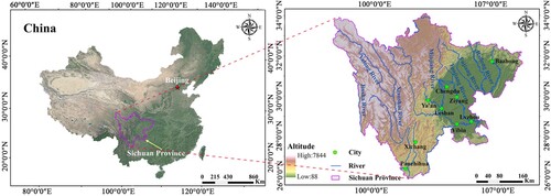
Sichuan Province is located in the southwestern part of China, covering an area of approximately 486,100 km² and extending between 97°21′ and 108°31′ E longitude and 26°03′ and 34°19′ N latitude (Figure 1). Due to the presence of extensive river networks, the study area has abundant water resources. The study area's topography and geomorphology are highly diversified, consisting of basins, mountains, hills, and plateaus. The Yunnan-Guizhou Plateau, the Bayankala Mountains, Min Mountains, and Daba Mountains, and the Tibetan Plateau form the southern, northern, and western borders of the study area, respectively. The general elevation of the study region ranges from 688 to 4,745 m above sea level. The slope gradient in this region was divided into seven categories, and 88.45% of the gradients were less than 38°. The study area included three main climate zones: the subtropical climate zone, alpine climate zone, and mid-subtropical humid climate zone. The climate of the study area is characteristic of a temperate continental monsoon zone, being warm in summer and cool in winter. According to a statistical analysis of long-term historical rainfall data (1979-2020) from the Sichuan Provincial Meteorological Service, the average annual rainfall is 1032.5 mm. The rainy season lasts from June to September, and rainfall during this period accounts for 70.25% of the total annual rainfall. There have been 186 major earthquakes (1128-2020) with a surface wave magnitude (Ms) greater than 5.0 recorded in this region, which indicates that the seismic activity is relatively strong.

Figure 1. Location of the study area.

3. Materials

3.1. Landslide inventory

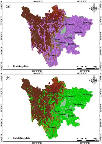
The construction of a landslide inventory is the basis of LSM. In addition to providing sample labels for the training of the proposed models, a landslide inventory can improve our comprehension of the spatial relationship between historical landslide occurrence and selected conditioning factors. A set of base maps relevant to landslide occurrence were used in this study, including the ALOS PALSAR digital elevation model (DEM), geology maps (1:200,000-scale), rainfall maps, and road maps. The Department of Natural Resources of Sichuan Province provided information on the historical distribution of landslides in Sichuan Province. Because of the large area of the study area and the huge amount of data involved, this study used the High-performance Computing Platform of Sichuan Agricultural University when analyzing the data. In the study area, a total of 34,893 landslide points were mapped, as shown in Figure 2. A total of 24,425 landslides (70%) were randomly chosen for model training, while the remaining 10,468 landslides (30%) were used for model validation to assess landslide susceptibility. The construction of nonlandslide points is important to suppress the overestimation of landslide susceptibility. However, there are currently no guidelines and no reasonable technique for obtaining nonlandslide points (Hu et al. 2020; Chang et al. 2023). In this study, nonlandslide points were chosen to meet the following requirements. First, every non-landslide point needs to be at least 500 m away from landslides. Second, any two nonlandslide points must be separated by a distance of greater than 100 meters. These requirements aid in preventing sampling in landslide-affected areas. A total of 34,893 nonlandslide points were generated from the nonlandslide area and divided into two subsets (70/30).

Figure 2. Landslide inventory map of the study area: (a) training data. (b) validating data.

3.2. Landslide conditioning factors

The environmental variables of landslide occurrences are essential for predicting landslide susceptibility (Lin et al. 2022). There are hundreds of conditioning factors that influence landslides (Reichenbach et al. 2018). The appropriate factors need to be chosen to create a trustworthy map of landslide susceptibility. However, there are no clear guidelines or uniform criteria for choosing conditioning factors. In this study, it was necessary to determine the landslide conditioning factors based on the regional geo-environment characteristics, an examination of the prior literature, and the availability of data sources for the study area. Fourteen landslide conditioning factors were selected for the spatial prediction of landslides: slope angle, road density, slope aspect, relief amplitude, cutting depth, elevation, surface roughness, stream power index (SPI), plan curvature, river density, peak ground acceleration (PGA), annual maximum 24-hour rainfall, profile curvature, and lithology (Table 2) used for landslide susceptibility modelling (Figure 3). The details of data collection are documented in Table 3.

Figure 3. Landslide influencing factor maps: (a) elevation. (b) slope angle. (c) slope aspect. (d) relief amplitude. (e) cutting depth. (f) river density. (g) plan curvature. (h) surface roughness. (i) profile curvature. (j) SPI. (k) rainfall. (l) lithology. (m) PGA. (n) road density.

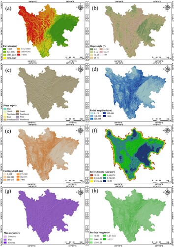
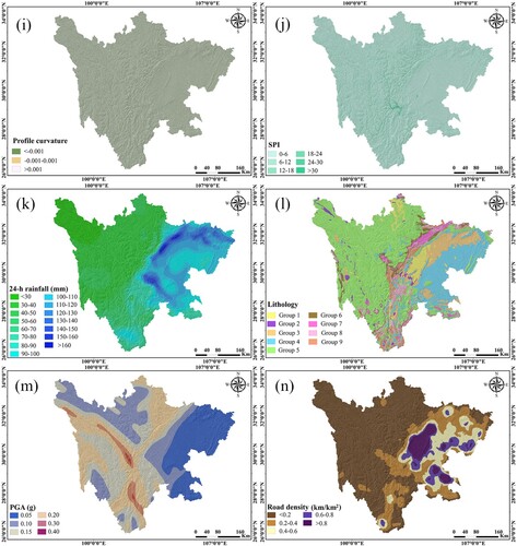
Table 2. Description of geological units of the study area.

Group	Code	Lithology	Geological age
Group 1	Q1^fp, Q2^fp, Q2^g, Q3^fl, Q3^fl, Q4^f	Gravel, sand, sandy gravel, clay	Quaternary
Group 2	N, E, R, γ5	Sandy conglomerate, shale, granite	Tertiary
Group 3	K1, K2, r3 5, γη3 5	Sandy conglomerate, mudstone, siltstone, sandstone, granite	Cretaceous
Group 4	J1, J1+2, J2, γη2 5, γδ2 5, J3 γη1 5, ηO2 5, δO1 5, γO1 5, T1-2, T2, T3, V1 5, P2T1, δ1 5	Mudstone, sandstone, limestone, granite, diorite	Jurassic
Group 5	γη1 5, CP, γδ1 5, γδ1 4, γ1 5, P1, P2, ϵO1 5, ϵ1 5	Monzonite, diorite, granite, gabbro, peridotite, limestone, sandstone, syenite	Triassic-Permian
Group 6	DC, βμ, δO4, σ4, βμ4, γσ4, D	Dolerite, diorite, peridotite, granite, dolomite, limestone, mudstone, sandstone, shale	Carboniferous-Devonian
Group 7	S, OS, S1+2, O, AnS	Slate, phyllite, tuff, shale, marl	Silurian-Ordovician
Group 8	Є, Z, Z1, Z2, Pt1, ZЄ	Limestone, dolomite, sandstone, sandy conglomerate, shale	Cambrian-Sinian
Group 9	Pt2, δ2, γη2, γ2, Ar3-Pt1	Diorite, griotte, gneiss, granite, andesite, slate	Pre-Sinian

Table 3. Data collection in this study.

Dataset	Factors	Scale/resolution	Data type
Landslide inventory^a	Landslide	/	Datasheet
Topographical map^b	Plan curvature	12.5 m	Grid
	Profile curvature	12.5 m	Grid
	Slope angle	12.5 m	Grid
	Slope aspect	12.5 m	Grid
	Relief amplitude	12.5 m	Grid
	Cutting depth	12.5 m	Grid
	River density	12.5 m	Grid
	Surface roughness	12.5 m	Grid
	Elevation	12.5 m	Grid
	SPI	12.5 m	Grid
Geological map^c	Lithology	1:200,000	Grid
Seismic map^d	PGA	1:200,000	Vector
Rainfall map^e	Rainfall	1:200,000	Grid
Road map^f	Road density	1:200,000	Vector

Data source: ^a: Department of Natural Resources of Sichuan Province, ^b: ALOS PALSAR DEM, ^c: China Geological Survey, ^d: China Geological Survey, ^e: Sichuan Provincial Meteorological Service, ^f: Google Earth© images.

Elevation is an important factor that is frequently used in LSM (Zhang et al. 2023). In this study, the elevation values of the study area were grouped into five classes: < 824 m, 824–1,581 m, 1,581–2,378 m, 2,378–3,142 m, 3,142–3,803 m, 3,803–4,341 m, and > 4,341 m (Figure 3(a)).

Slope angle is an essential conditioning factor in landslide susceptibility evaluations, as it is directly tied to the forces that cause hill slopes to shift (Bozzolan et al. 2023). The slope angle values for this study were reclassified into seven classes (Figure 3(b)).

Slope aspect describes the degree of solar radiation received on slope faces, which can affect soil moisture and slope stability (Zhang et al. 2023). The slope aspect map, as shown in Figure 3(c), was divided into nine categories, including eight directions and flat.

Relief amplitude, the altitude difference between a given area's highest and lowest points, is another important factor for landslide susceptibility modeling (Huang et al. 2020). The relief amplitude map was divided into five classes for this study: < 118 m, 118–222 m, 222–338 m, 338–446 m, and > 446 m (Figure 3(d)).

Cutting depth is defined as the difference between the average and lowest elevations in a certain area and is a frequently utilized component in LSM (Chen et al. 2022). The cutting depth map was divided into six categories: < 102 m, 102–188 m, 188–275 m, 275–382 m, 382–491 m, and > 491 m (Figure 3(e)).

River density, defined as the total length of a river network in a given area, is another important topographical factor in LSM (Alqadhi et al. 2021). For this study, the river density of the study area was divided into six classes: < 0.38 km/km², 0.38–0.52 km/km², 0.52–0.64 km/km², 0.64–0.74 km/km², 0.74–0.83 km/km², and > 0.83 km/km² (Figure 3(f)).

Plan curvature has a direct impact on the convergence and divergence of water flow across a surface, which in turn affects the process of landsliding (Al-Najjar and Pradhan 2021). The plan curvature map was divided into three classes: flat, concave, and convex (Figure 3(g)).

Surface roughness is considered a significant conditioning factor affecting landslide susceptibility (Abdulwahid and Pradhan 2017). This factor was grouped into five categories as follows: < 1.00, 1.00–1.10, 1.10–1.23, 1.23–1.52, and > 1.52 (Figure 3(h)).

Profile curvature influences the acceleration and deceleration of stream movement and is an essential indicator of erosion and sediment movement (Al-Najjar and Pradhan 2021). This factor was classified into three classes: <− 0.001, −0.001–0.001, and >0.001 (Figure 3(i)).

SPI describes the erosion ability of surface water and thus influences the probability of a landslide occurrence within the study area (Zhou et al. 2021). The SPI map was constructed into six categories: 0–6, 6–12, 12–18, 18–24, 24–30, and >30 (Figure 3(j)).

Rainfall is recognized as one of the most important variables in the development of landslides since it affects slope shear strength (Huang et al. 2022). In this study, the annual maximum 24-hour rainfall was utilized to map landslide susceptibility, and the rainfall map was classified into fifteen classes with 10 mm intervals (Figure 3(k)).

Lithology is one of the most commonly used variables in landslide susceptibility studies, and some geological formations are more conducive to landslides (Chen et al. 2022). There are nine major lithological groups in the study area (Figure 3(l)).

PGA is regarded as an essential dynamic component for assessing the influence of earthquakes on landslides (Yi et al. 2019). For the study area, the PGA ranges from 0.05 to 0.4 g (Figure 3(m)).

Road density represents the connection between anthropogenic activities and landslide occurrence, and it influences slope stability (Abedini et al. 2019). The road density map in the study area was constructed with five categories: < 0.2 km/km², 0.2–0.4 km/km², 0.4–0.6 km/km², 0.6–0.8 km/km², and > 0.8 km/km² (Figure 3(n)).

4. Methods

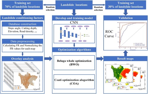
4.1. General methodology

The methodology for this study included five major steps: (1) database preparation, (2) mapping a set of conditioning factors, (3) designing and training predictive models, (4) generating surface maps of landslide susceptibility, and (5) evaluating the models and maps quantitatively (Figure 4). The frequency ratio (FR) model, which can represent the spatial correlations between landslide distribution and each conditioning factor, was used to identify geographic information system (GIS) factors related to landslide incidence (Berhane, Kebede, and Alfarrah 2021). The FR represents the probability ratio of a landslide occurrence to a nonoccurrence for a particular attribute (Guo et al. 2021). The ratio can be calculated as follows: (1) $F{R}_i={\displaystyle \frac{G_i/G}{H_i/H}}$(1) where G_i is the number of landslide pixels in each subclass i of a conditioning factor, G is the total number of landslide pixels, H_i is the number of pixels of each subclass i, and H is the number of total pixels in the study area.

Figure 4. Methodological flow chart of the present study.

4.2. Evaluation of conditioning factors

In LSM, the quality of the map depends on both the selected models and the data's capacity for prediction. Since not all landslide conditioning factors have the same level of predictive power, some factors may produce noise that lowers the predictive ability of the final models (Tien Bui et al. 2016). Conditioning factors with little or no predictive power should be eliminated to achieve more accurate results. In this study, the linear support vector machine (LSVM) model was employed to examine the prediction capability of the fourteen conditioning factors. The classification accuracy of this model could be improved by removing unnecessary input parameters (Roy et al. 2020). Quantification of the prediction capabilities of the fourteen conditioning factors was carried out using the following equation (Pham et al. 2017): (2) $g(x)=\mathrm{sgn}(w^{T}m+n)$(2) where w^T is the inverse matrix, m = (m₁, m₂, … , m₁₄) is the input vector containing fourteen conditioning factors, and n is the offset from the origin of the hyperplane. Average Merit (AM) is a quantitative measure for determining the relative significance of conditioning factors. The higher the AM for each conditioning factor, the greater its influence on the occurrence of landslides.

4.3. Convolutional neural network (CNN)

CNN is a well-known deep learning method that can automatically extract useful features from hierarchical neural networks (Li et al. 2022). A basic CNN model is made up of several neural layers, which commonly include convolution layers, pooling layers, and fully connected layers (Figure 5). The convolutional layer can simultaneously find connections between each feature class and perform well by leveraging information extracted from the input data. The pooling layer allows the neural network to focus more on important features by lowering the number of features. Maximum pooling and average pooling are the two most common pooling techniques (Momeny et al. 2022). Maximum pooling uses the maximum value of the features, while average pooling uses the features’ average value within a specific pooling zone. The fully connected layer is often used to construct the final combination of nonlinear properties to predict the network design's end. The convolutional layer in the CNN approach employs a set of convolution kernels to learn an efficient appearance from input variables. Assume that v = {v₁, v₂, … , v_N} refers to the input feature vectors, where N is the number of conditioning factors. Assume that the convolutional layer contains k kernels, with the jth kernel having the weight and bias w_j and b_j, respectively. As a result, the convolutional operation's output C_j can be calculated using the following equation (Xie et al. 2023): (3) $C_j=\sum _i^{N}f(w_j\ast v_i+b_j),j=1,2,\dots ,k$(3) where * stands for the convolutional operation and f is the nonlinear activation function.

Figure 5. CNN structure.

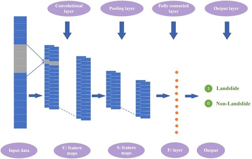
To reduce the size of the feature vector and avoid overfitting, the pooling layer (max-pooling), which comes after the convolution layer, was used. The extracted feature vectors are then reorganized by fully connected layers. Finally, using the softmax activation function, the detected vector is transformed into a prediction probability for the related category. The probability is calculated as follows: (4) $p(y=mX)={\displaystyle \frac{\exp (w_{m}X+b_m)}{\sum _{n=1}^M\exp (w_{n}X+b_n)}}$(4) where m is the predicted class, M represents the number of categories, w_m and w_n represent the weight vectors, and b_m and b_n indicate the bias vectors.

4.4. Metaheuristic optimization algorithms

4.4.1. Beluga whale optimization (BWO)

The BWO algorithm is a novel swarm-based metaheuristic algorithm inspired by the natural behavior of beluga whales (Zhong, Li, and Meng 2022). BWO, similar to other metaheuristic algorithms, includes the exploration phase and the exploitation phase (Figure 6). The principle steps of the BWO are formulated as follows (Figure 7):

Figure 6. Beluga whale behaviors include (a) the exploration phase, (b) the exploitation phase, and (c) the whale fall phase (modified after Zhong, Li, and Meng 2022).

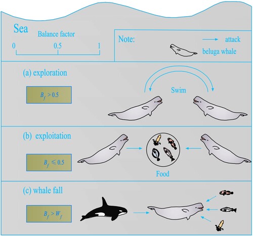
Figure 7. Flowchart of the BWO (modified after Zhong, Li, and Meng 2022).

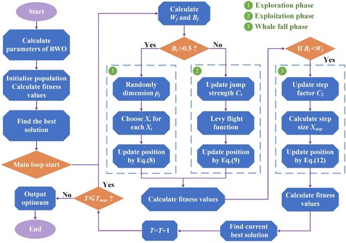
Initialization stage: Due to the population-based nature of BWO, beluga whales are used as search agents. Each beluga whale is a potential solution that is updated during optimization. The matrix of search agent positions is represented as: (5) $X=\left[\begin{array}{cccc}{x}_{1,1}& x_{1,2}& \cdots & x_{1,d}\\ x_{2,1}& x_{2,2}& \cdots & x_{2,d}\\ ⋮& ⋮& ⋮& ⋮\\ x_{n,1}& x_{n,2}& \cdots & x_{n,d}\end{array}\right]$(5) where n represents the population size of the search agents and d stands for the design variables’ dimensionality.

The relevant fitness values for each beluga whale are stored as follows: (6) $F_x=\left[\begin{array}{c}f(x_{1,1},x_{1,2},\dots \dots ,x_{1,d})\\ f(x_{2,1},x_{2,2},\dots \dots ,x_{2,d})\\ ⋮\\ f(x_{n,1},x_{n,2},\dots \dots ,x_{n,d})\end{array}\right]$(6) The balance factor B_f can be denoted as: (7) $B_f=B_0(1-T/2T_{max})=\{\begin{array}{cc}>0.5,& \mathrm{exploration}\mathrm{stage}\\ \le 0.5,& \mathrm{exploitation}\mathrm{stage}\end{array}$(7) where T_max is the current iteration's (T) maximum number of iterations. In each iteration, B₀ is a random number between (0, 1) that is created. The fluctuation range of B_f decreases from (0, 1) to (0, 0.5) as iteration T rises, showing the considerable change in probabilities for the exploitation and exploration phases, while the probability of the exploitation phase rises as iteration T rises.

Exploration stage: The formulation of the BWO's exploration stage includes an examination of the beluga whales’ swimming behavior. The positions of the beluga whales are established by their pair swim, and these positions are modified as follows: (8) $\{\begin{array}{cc}{X}_{i,j}^{T+1}=X_{i,p_j}^T+(X_{r,p_1}^T-X_{i,p_j}^T)(1+r_1)\sin (2\pi r_2),& j=\mathrm{even}\\ X_{i,j}^{T+1}=X_{i,p_j}^T+(X_{r,p_1}^T-X_{i,p_j}^T)(1+r_1)\cos (2\pi r_2),& j=\mathrm{odd}\end{array}$(8) where T is the latest iteration, $X_{i,j}^{T+1}$ denotes the i-th beluga whale's new location on the jth dimension, and p_j denotes a random number drawn from the jth set. The current locations for the rth and ith are represented by $X_{r,P1}^T$ and $X_{i,Pj}^T$, respectively, where r is a randomly chosen beluga whale, r₁ and r₂ are random numbers between (0, 1), and $\cos (2\pi r_2)$ and $\sin (2\pi r_2)$ reveal that the fins of the mirrored beluga whales face upward.

Exploitation stage: This stage takes cues from beluga whales’ hunting behaviors. Beluga whales can migrate and forage together depending on their proximity to other beluga whales. Thus, beluga whales hunt by sharing information about available positions for each other and choosing the best candidate among them. To improve convergence, a Levy flight technique is added to the BWO exploitation step and is represented as: (9) $X_i^{T+1}=r_3{X}_{\mathrm{best}}^T-r_4{X}_i^T+C_1.L_f.(X_r^T-X_i^T)$(9) where $X_i^T$ and $X_r^T$ represent the current positions of the ith beluga whale and a random beluga whale, respectively; $X_i^{T+1}$ and $X_{\mathrm{best}}^T$ represent the ith beluga whale's new position and the best position for the entire population; r₃ and r₄ represent random numbers between (0, 1); and $C_1=2r_4(1-T/T_{max})$ represents the random jump strength.

The Levy flight function, or L_f, is computed as follows: (10) $L_f=0.05\times {\displaystyle \frac{u\times \sigma }{{|v|}^{1/\beta }}}$(10) (11) $\sigma ={\left({\displaystyle \frac{\mathrm{\Gamma }(1+\beta )\times \sin (\pi \beta /2)}{\mathrm{\Gamma }((1+\beta )/2)\times \beta \times 2^{(\beta -1)/2}}}\right)}^{1/\beta }$(11) where β is a constant set to 1.5 and u and v are random values with a normal distribution.

Whale fall: Killer whales, polar bears, and people pose threats to beluga whales throughout their migration and foraging. The majority of beluga whales are clever and can avoid danger by sharing information with one another. Nevertheless, a small number of beluga whales did not thrive and died on the deep seabed. The phenomenon, known as ‘whale fall,’ provides food for a variety of creatures. The BWO replicates the whale fall process by selecting the probability of whale fall from the population's individuals. Based on the probability of the whale fall that was chosen to handle every change in all groups, it is considered that these beluga whales either migrated or fell into the deep sea. In order to keep the population size constant, the positions of beluga whales and the step size at which a whale falls are used to determine the updated position. The mathematical formulation of the model is as follows: (12) $X_i^{T+1}=r_5{X}_i^T-r_6{X}_r^T+r_7{X}_{\mathrm{step}}$(12) where r₅, r₆ and r₇ represent random numbers between (0, 1), and X_step is the whale fall's step size and can be expressed as follows: (13) $X_{\mathrm{step}}=(u_b-l_b)\exp (-C_{2}T/T_{max})$(13) (14) $C_2=2W_f\times n$(14) where C₂ is the step factor that correlates with the likelihood of whale falls and population size, and u_b and l_b are the upper and lower variable boundaries, respectively. It is clear that the maximum number of iterations, the iterations, and the boundaries of the design variables all have an influence on C₂.

The probability of a whale falling (W_f) is calculated as a linear function in the BWO model: (15) $W_f=0.1-0.05T/T_{max}$(15) The likelihood of whale fall drops from 0.1 in the first iteration to 0.05 in the last iteration, indicating that the risk of beluga whales decreases as they get closer to their food source during the optimization process.

4.4.2. Coati optimization algorithm (COA)

The COA algorithm is a brand-new bioinspired optimization algorithm inspired by Coati's natural behavior (Dehghani et al. 2023). The fundamental idea of COA is the replication of the two natural behaviors of coatis: (i) pursuing and attacking iguanas and (ii) fleeing from predators. In the COA algorithm, coatis are viewed as population participants. Each coati's position in the search space determines the values for the decision factors. Therefore, the coatis’ position in the COA offers a potential solution to the problem. The coatis’ initial position in the search space is created at random using the following equation: (16) $X_i:X_{i,j}=l{b}_j+r\cdot (u{b}_j-l{b}_j),i=1,2,\dots ,N,j=1,2,\dots ,m$(16) where X_i is the ith coati's position in the search space, x_i,j is the jth decision variable's value, N is the number of coatis, m is the number of decision variables, r is a random number between (0, 1), and lb_j and ub_j are the lower and upper boundaries of the jth decision variable, respectively.

The population matrix (X) is a mathematical representation of the coati population in the COA and can be obtained as follows: (17) $X={\left[\begin{array}{c}{X}_1\\ ⋮\\ X_i\\ ⋮\\ X_N\end{array}\right]}_{N\times m}={\left[\begin{array}{ccccc}{x}_{1,1}& \cdots & x_{1,j}& \cdots & x_{1,m}\\ ⋮& \ddots & ⋮& .& ⋮\\ x_{i,1}& \cdots & x_{i,j}& \cdots & x_{i,m}\\ ⋮& .& ⋮& \ddots & ⋮\\ x_{N,1}& \cdots & x_{N,j}& \cdots & x_{N,m}\end{array}\right]}_{N\times m}$(17) Different values for the problem's objective function are evaluated as a result of the placement of potential solutions in decision variables. These values can be given as follows: (18) $F={\left[\begin{array}{c}{F}_1\\ ⋮\\ F_i\\ ⋮\\ F_N\end{array}\right]}_{N\times 1}={\left[\begin{array}{c}F(X_1)\\ ⋮\\ F(X_i)\\ ⋮\\ F(X_N)\end{array}\right]}_{N\times 1}$(18) where F_i is the objective function value derived based on the ith coati, and F is the vector of the obtained objective function.

The COA population is updated in two different stages. The two stages of the COA are formulated as follows (Figure 8):

Figure 8. Flowchart of the COA (modified after Dehghani et al. 2023).

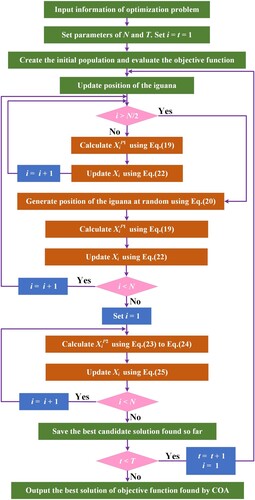
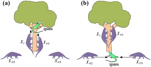
Hunting and attacking strategy on iguana (exploration stage): The initial stage of updating the number of coatis in the search space is based on modeling their attack strategy on iguanas. In this method, several coatis climb up the tree to approach an iguana and startle it. Other coatis gather around the iguana as it falls to the ground while they wait under a tree. The iguana falls to the ground, and the coatis attack and hunt it. The pattern diagram for this strategy is shown in Figure 9. It is assumed that the iguana occupies the position of the best member of the population. The following equation is used to approximate the coatis’ location when they emerge from the tree. (19) $X_i^{P1}:x_{i,j}^{P1}=x_{i,j}+r\cdot (\mathrm{Iguan}{\mathrm{a}}_j-I\cdot x_{i,j}),\mathrm{for}i=1,2,\dots ,\lfloor {\displaystyle \frac{N}{2}}\rfloor \mathrm{and}j=1,2,\dots ,m.$(19) When the iguana falls to the ground, it is randomly placed in the search space. Coatis on the ground move in the search space according to this random position, which is approximated using Eqs. (20) and (21). (20) ${\mathrm{Iguana}}^G:{\mathrm{Iguana}}_j^G=l{b}_j+r\cdot (u{b}_j-l{b}_j),j=1,2,\dots ,m,$(20) (21) $\begin{array}{c}{X}_i^{P1}:x_{i,j}^{P1}=\{\begin{array}{cc}{x}_{i,j}+r\cdot (\mathrm{Iguan}{a}_j^G-I\cdot x_{i,j}),& F_{{\mathrm{Iguana}}^G<}<F_i,\\ x_{i,j}+r\cdot (x_{i,j}-\mathrm{Iguan}{a}_j^G),& \mathrm{else},\end{array}\\ \mathrm{for}i=\lfloor {\displaystyle \frac{N}{2}}\rfloor +1,\lfloor {\displaystyle \frac{N}{2}}\rfloor +2,\dots ,N\mathrm{and}j=1,2,\dots ,m.\end{array}$(21) If the new location estimated for each coati improves the value of the goal function, it is acceptable for the update process. Otherwise, the coati stays in its former position. This update condition is simulated using Eq. (22) for i = 1, 2, … , N. (22) $X_i=\{\begin{array}{cc}{X}_i^{P1},F_i^{P1}<F_i& \\ X_i,\mathrm{else}.& \end{array}$(22) where n represents the population size of the search agents and d stands for the design variables’ dimensionality.

Figure 9. Pattern diagram for the Coati Optimization Algorithm's first stage (modified after Dehghani et al. 2023): (a) Attack of half of the coatis’ population towards the iguana on the tree; (b) Hunting the fallen iguana by the other half of the coatis’ population.

Here, $X_i^{P1}$ is the newly determined position for the ith coati, $X_{i,j}^{P1}$ is its jth dimension, $F_i^{P1}$ is the value of its objective function, r is a random real number between (0, 1), and Iguana stands for the position of the iguana in the search space, which actually corresponds to the position of the best member. Iguana_j is its jth dimension, I is an integer that is randomly chosen from the set {1, 2}, Iguana^G is the randomly generated iguana's position on the ground, Iguana_j^G is its jth dimension, $F_{Iguan{a}^G}$ is its objective function value, and ⌊·⌋ is the floor function.

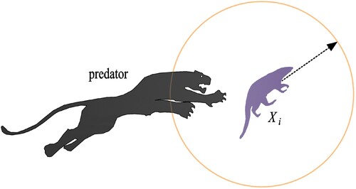
The process of escaping from predators (exploitation stage): The second stage of the process of updating coatis’ positions in the search space is mathematically modeled based on coatis’ typical behavior when encountering and evading predators. When a predator attacks a coati, it leaves its location (Figure 10). Coati's actions in this method place it in a secure position close to its current position, demonstrating the COA's ability for local search exploitation. To imitate this behavior, a random position near the position of each coati is generated using Eqs. (23) and (24). (23) $l{b}_j^{\mathrm{local}}={\displaystyle \frac{l{b}_j}{t},u{b}_j^{\mathrm{local}}={\displaystyle \frac{u{b}_j}{t},\mathrm{where}t=1,2,\dots ,T.}}$(23) (24) $\begin{array}{c}{X}_i^{P2}:x_{i,j}^{P2}=x_{i,j}+(1-2r)\cdot (l{b}_j^{\mathrm{local}}+r\cdot (u{b}_j^{\mathrm{local}}-l{b}_j^{\mathrm{local}}))\\ i=1,2,\dots ,N,j=1,2,\dots ,m\end{array}$(24)

Figure 10. Pattern diagram of a coati evading a predator in the second phase of Coati Optimization Algorithm (modified after Dehghani et al. 2023).

If the newly calculated position enhances the value of the objective function, this condition uses Eq. (25), then it is acceptable. (25) $X_i=\{\begin{array}{cc}{X}_i^{P2},F_i^{P2}<F_i& \\ X_i,\mathrm{else}.& \end{array}$(25) Here, $X_i^{P2}$ is the new location determined for the ith coati, $X_{i,j}^{P2}$ is its jth dimension, $F_i^{P1}$ is the value of its objective function, r is a random number between (0, 1), t is the iteration timer, the jth decision variable's local lower and upper bounds are denoted as lb_j^local and ub_j^local, respectively, and lb_j and ub_j represent the jth decision variable's lower and higher bounds.

4.5. Model evaluation measures

The accuracy of measurement results in LSM should be ensured through model performance evaluation. The confusion matrix was utilized in this study to assess the performance of all models. Based on the confusion matrix, several performance metrics were obtained, including specificity (SPF), sensitivity (SST), accuracy (ACC), Cohen’s kappa coefficient (κ), positive predictive value (PPV), and negative predictive value (NPV). These performance metrics can be calculated using the following equations: (26) $PPV={\displaystyle \frac{TP}{TP+FP}}$(26) (27) $NPV={\displaystyle \frac{TN}{TN+FN}}$(27) (28) $SST={\displaystyle \frac{TP}{TP+FN}}$(28) (29) $SPF={\displaystyle \frac{TN}{TN+FP}}$(29)

(30) $ACC={\displaystyle \frac{TP+TN}{TP+TN+FP+FN}}$(30) (31) $\kappa ={\displaystyle \frac{ACC-AC{C}_{\exp }}{1-AC{C}_{\exp }}}$(31) (32) $P_{\exp }={\displaystyle \frac{(\mathrm{TP}+\mathrm{FN})(\mathrm{TP}+\mathrm{FP})+(\mathrm{FP}+\mathrm{TN})(\mathrm{FN}+\mathrm{TN})}{{(TP+TN+FP+FN)}^2}}$(32) where TP, TN, FP, and FN are true positive, true negative, false positive, and false negative, respectively.

The ROC curve is another method for validating the overall performance of a model. Plotting SST against 100-SPF based on a variety of different dichotomies yields the ROC curve. The statistical summary of the overall effectiveness of method performances is represented by the AUC index. The AUC value typically varies from 0.5 to 1. A larger AUC value always indicates better model performance. Additionally, the root mean square error (RMSE) is one of the most helpful indicators when high errors are primarily undesirable. The value of RMSE is inversely correlated with the model's accuracy, and a smaller value of RMSE indicates a model that performs better. RMSE was determined for the current study using the following formula: (33) $RMSE=\sqrt{{\displaystyle \frac{1}{n}\sum _{i=1}^n{(y_{pred}-y_{tru})}^2}}$(33) where n is the total sample size for the training and testing dataset, y_pred denotes the predicted value, and y_tru denotes the truth value.

5. Results

5.1. Factor assessment results

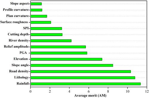
Based on average merit (AM), each conditioning factor's effectiveness was rated in the current study using the LSVM model. Figure 11 shows the AM of each conditioning factor. The estimated AM value illustrates the chosen factor's capacity for influence. The landslide susceptibility model is more effectively built when the AM value is higher. According to the feature selection results, rainfall (AM = 11.34) is the most crucial factor for landslide modeling, followed by lithology (10.77), road density (10.33), slope angle (8.49), elevation (7.37), PGA (5.82), relief amplitude (5.68), river density (4.20), cutting depth (3.27), SPI (3.22), surface roughness (2.09), plan curvature (1.68), profile curvature (1.18), and slope aspect (1.13). Overall, all fourteen landslide conditioning factors contributed positively to the occurrence of landslides (AM > 0). As a result, all of these factors were chosen for present landslide modeling.

Figure 11. Average merit of the landslide conditioning factors.

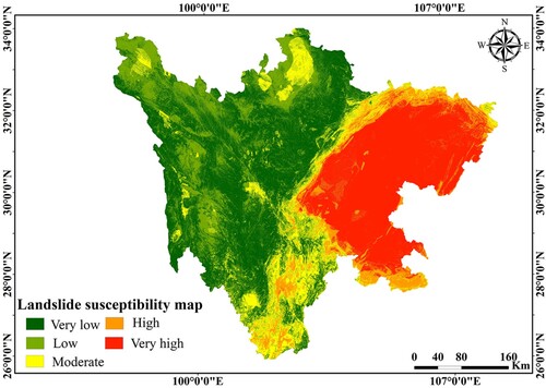
5.2. Landslide susceptibility maps

To find differences in landslide susceptibility across the entire study area, the output values of the three models were recategorized into the following five levels: very low, low, moderate, high, and very high (Figures 12–14). The spatial distribution of landslide susceptibility is similar in all three models. The majority of past landslides fall into high- and very high-susceptibility areas as a whole. The eastern part of Sichuan Province has the highest risk of sliding, and the three models are extremely vulnerable. Some landslide conditioning factors, such as rainfall (90–130 mm), lithology (Group 3 and Group 4), road density (0.2–0.6 km/km²), slope angle (9–24°), and altitude (< 2,378 m), may play an important role in the emergence of very high and highly susceptible areas. Heavy rain that falls continuously has the potential to saturate the rock and soil mass, create positive pore pressure, and act as a catalyst for other conditions to come together more quickly and cause a landslide. The lithological unit has a significant impact on the occurrence of landslides. In Sichuan Province, the Jurassic and Cretaceous strata composed of sandstone intercalated with a high percentage of mudstone are known as the most slide-prone strata and have produced numerous landslides. Engineering construction connected with road networks has significantly altered local landforms and the hydrogeological characteristics of slopes, weakening slope stability. The equilibrium of natural slopes is disturbed by the inappropriate excavation of the slope toe, which promotes the formation of landslides. Changes in slope angle have a direct impact on the shear stress, which leads to failures. Compared to hard rocks, weak rocks were unable to withstand the higher slope angle. Sichuan Province is dominated by gentle and medium slope angles. A total of 77.25% of all landslides are located in the slope gradient range of < 24°, which makes up 59.73% of the gradients in the region. Landslides appear to be associated with medium or moderate slopes, which have the characteristics of slide-type movements. Higher slopes are related to rock falls and avalanches, while lower slopes are related to flow-type movements. The low frequency of landslides on steeper slopes is mostly due to a low number of such cells. Additionally, the research area's steep natural slopes are not prone to landslides because they are mostly made of bedrock with high weathering resistance. Low-altitude regions are more likely to experience landslides than high-altitude regions. These regions have a high concentration of human activity, which increases the risk of landslides. The best strategy to prevent landslides is to pay closer attention to the co-occurrences of the landslide-related factors outlined above. The low and very low susceptibility zones are primarily found in the research area's west and north, with high altitudes and steep slope angles, and these characteristics are inappropriate for the occurrence of landslides.

Figure 12. Landslide susceptibility map produced by the CNN model.

Figure 13. Landslide susceptibility map produced by the CNN-BWO model.

Figure 14. Landslide susceptibility map produced by the CNN-COA model.

5.3. Model validation and comparison

Tables 4 and 5 show the training and validation performances of three landslide models employing PPV, NPV, SST, SPF, ACC, and κ. The statistical index metrics for the CNN-COA model performed the best on the training dataset, followed by the CNN-BWO model and the CNN model. As shown by the kappa indices of 0.867, 0.832, and 0.730 for the CNN-COA, CNN-BWO, and CNN models, respectively, there is substantial agreement between the observed and projected landslides. The results of the validation dataset follow the same pattern as the training dataset. Figure 15 shows the ROC plots for the CNN-COA, CNN-BWO, and CNN models, and Tables 6 and 7 show the detailed results. The CNN-COA model has the highest predictive performance for the training dataset, as evidenced by its higher AUC value (0.946) compared to the other two models. When compared to the training dataset, the results of the validation dataset revealed similar performance trends. The CNN-COA model (0.919) had the greatest AUC value, followed by the CNN-BWO model (0.906) and the CNN model (0.805). In general, all landslide models perform well in the assessment of landslide susceptibility (AUC > 0.8).

Figure 15. Comparison of the three models using ROC curve technique with (a) the training dataset and (b) the validation dataset.

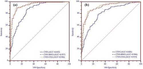
Table 4. Model performance on the training dataset.

Models	PPV	NPV	SST	SPF	ACC	κ
CNN-COA	0.953	0.905	0.909	0.951	0.929	0.867
CNN-BWO	0.947	0.901	0.907	0.944	0.924	0.832
CNN	0.881	0.836	0.843	0.876	0.859	0.730

Table 5. Model performance on the testing dataset.

Models	PPV	NPV	SST	SPF	ACC	κ
CNN-COA	0.936	0.884	0.889	0.933	0.909	0.838
CNN-BWO	0.918	0.871	0.877	0.914	0.894	0.792
CNN	0.830	0.792	0.797	0.824	0.811	0.665

Table 6. AUC analysis for the nine landslide models with the training dataset.

Models	AUC	SE	95%CI
CNN-COA	0.946	0.0136	0.912–0.970
CNN-BWO	0.937	0.0152	0.901–0.964
CNN	0.855	0.0230	0.806–0.895

Table 7. AUC analysis for the nine landslide models with the testing dataset.

Models	AUC	SE	95%CI
CNN-COA	0.919	0.0173	0.879–0.949
CNN-BWO	0.906	0.0188	0.864–0.939
CNN	0.805	0.0268	0.752–0.852

By comparing the standard error (SE) and 95% confidence interval (CI), the CNN-COA model has the smallest SE (0.0136) and the narrowest 95% CI (0.912–0.970), followed by the CNN-BWO model (SE = 0.0152; 95% CI = 0.901–0.964) and the CNN model (SE = 0.0230; 95% CI = 0.806–0.895). The CNN-COA model has the best performance among the three models, and the training datasets of all three models show a respectable goodness of fit. The established model's results were verified using the validation dataset, and the CNN-COA model still had the smallest SE (0.0173) and the narrowest 95% CI (0.879-0.949). The GD-FFR-RF model clearly outperforms the other two models when using the validation dataset.

6. Discussion

By choosing the appropriate landslide conditioning factors, landslide susceptibility models can produce more accurate findings with less noise, improving their prediction power. Therefore, in landslide modeling or landslide susceptibility studies, the choice of proper conditioning factors is seen as a crucial issue. Due to the complexity of landslides, there was no established global protocol or clear guidelines for choosing trustworthy landslide conditioning factors in earlier studies. According to Wang et al. (2020), the random forest model can be used to choose the landslide conditioning variables. Their findings demonstrate that the catchment area indicated a nonpredictive value; therefore, these values were eliminated from the landslide susceptibility modeling. To improve the performance of the landslide model, Chen et al. (2022) used the information gain ratio method to exclude irrelevant or insignificant components. Other approaches, such as Relief-F (Fang et al. 2021), correlation attribute evaluation (Wu et al. 2020), and gain ratio (Wang, Fang, and Hong 2019), have also been used to identify landslide conditioning factors. Higher AUCs, reduced RMSE, and other metrics show that these strategies have indeed enhanced the performance of the landslide models. The LSVM model was used in the current study to rank the significance of conditioning factors. In the study area, rainfall was found to be the most significant factor influencing the occurrence of landslides. The result is in accordance with other authors such as Pham, Prakash, and Bui (2018), Jiao et al. (2019), Dou et al. (2020), Wang et al. (2020), and Mandal, Saha, and Mandal (2021). In reality, the hourly rainfall intensity is the primary driver of geological hazards such as flash floods and landslides. The annual maximum 24-hour rainfall has high importance in LSM, and the contribution of this factor to landslide occurrence varies by region. Rainfall infiltration alters the stresses inside the internal structure of slopes, reduces their shear strength, and causes slope instability. The results of the LSVM approach revealed that all of the conditioning factors were capable of positive prediction. Therefore, susceptibility models were created using all fourteen conditioning factors.

The CNN model is currently regarded as a superior landslide modeling tool across the globe due to its promising results and greater prediction rate in the spatial prediction of landslides (Aslam, Zafar, and Khalil 2023). For example, Sameen, Pradhan, and Lee (2020) used several models to assess landslide susceptibility. They found that a CNN-based model achieved the highest validation data accuracy (83.11%) and AUC (0.880). Mandal, Saha, and Mandal (2021) successfully investigated the landslide susceptibility of the Rorachu River basin. It also noted that the CNN model outperformed other machine learning algorithms such as random forest, artificial neural network, etc. A regional multihazard (flash floods, debris flows, and landslides) susceptibility prediction framework is provided by Ullah et al. (2022) for the Shangla District, Pakistan, based on three different models (CNN, logistic regression, and K-nearest neighbor). Their results show that the CNN model performs better than traditional machine learning models at estimating the susceptibility of flash floods, debris flows, and landslides. The CNN model's output should be regarded with caution because it frequently relies on parameters that have been predetermined and/or determined through trial and error. The CNN model's performance is mostly determined by its design, which includes the training approach, input window size, and layer depth. Metaheuristic optimization algorithms have been demonstrated to effectively increase landslide prediction accuracy (Jaafari et al. 2022). Those with optimum hyperparameters offer high-quality classification outputs and have the most potential for usage in LSM. In general, the model's structure, dataset size and quality, and parameter tuning can all affect how well a deep learning model predicts. Fine-tuning of the hyperparameters of the CNN model using metaheuristic techniques and the size of the input data influence the model's prediction performance (Table 8). Due to the COA algorithm's properties, CNN-COA outperformed the other algorithms in terms of prediction capacity. The ability to avoid local minima, accelerate convergence, and have superior robustness and stability due to only two control parameters needing to be tuned in the algorithm results in acceptable performance in predicting landslide susceptible areas.

Table 8. Hypermeters settings of the used models.

	Parameter settings	CNN	CNN-BWO	CNN-COA
Convolutional layer	Number of filters	8	32	32
	Filter size	3 × 3	7 × 7	7 × 7
	Activation function	ReLU	ReLU	ReLU
	Dropout rate	0.2	0.2	0.2
	Pooling type	max pooling	max pooling	max pooling
Fully connected layer	Number of nodes	3	5	5
	Activation function	Sigmoid	Sigmoid	Sigmoid
	Dropout rate	0.2	0.2	0.2

Several statistical indices showed that the CNN-COA model outperformed the other models on the training dataset. A total of 95.3% (PPV) and 90.5% (NPV) of the training dataset's pixels were correctly identified by the CNN-COA model as landslide and nonlandslide, respectively. For the classification of landslide locations, the CNN-COA (SST = 90.9%) model outperforms the CNN-BWO (SST = 90.7%) and CNN (SST = 84.3%) models. In terms of nonlandslide classification, the CNN-COA model still has the highest SPF (SPF = 95.1%), followed by the CNN-BWO model (SPF = 94.4%) and the CNN model (SPF = 87.6%). Additionally, the CNN-COA model outperformed the other two models, as shown by the results of ACC and κ. The results of all statistical indices in the validation dataset revealed that the CNN-COA model performed best (PPV = 93.6%, NPV = 88.4%, SST = 88.9%, SPF = 93.3%, ACC = 90.9%, and κ =  0.838). On both the training and validation datasets, two hybrid models (i.e. CNN-COA and CNN-BWO) demonstrated superior predictive performance.

The AUC value of the CNN model was increased by 9.1% and 8.2%, respectively, by the COA algorithm and the BWO algorithm utilizing the training dataset. COA and BWO both enhanced the CNN model's prediction by 11.4% and 10.1%, respectively. The RMSE value of each algorithm was used to conduct a second model performance study, with lower RMSE values indicating higher predicted accuracy. The RMSE values of the CNN, CNN-BWO, and CNN-COA models for the training dataset are 0.219, 0.094, and 0.083, respectively (Figures 16–18). The RMSE values for the CNN, CNN-BWO, and CNN-COA models for the validation dataset are 0.221, 0.124, and 0.084, respectively. These results demonstrate the COA algorithm's superior capacity to optimize the input dataset. As a result, in this instance, the COA algorithm is more suitable to create the hybrid model with the CNN. It should be emphasized that the CNN-BWO model can also yield satisfying results, which are just slightly inferior to the results of the CNN-COA model. The difference in performance with the training and validation datasets between the two innovative hybrid models is not substantial, and both models can give appropriate results to estimate landslide susceptibility in this study region. The difference in AUC values for the CNN model between the training and validation datasets was 0.050, and the corresponding differences of the CNN-BWO and CNN-COA models were 0.031 and 0.027, respectively. This shows that the risk of overfitting is more likely to occur in a single model, and the CNN-BWO and CNN-COA models can effectively avoid this issue by lowering the model's variance. In practice, the model's stability is crucial for landslide susceptibility modeling. Limitations can be used to express stability. For example, compared to the CNN model, the CNN-BWO and CNN-COA models need a relatively longer training time. As a result, model selection is relatively subjective depending on the perspective of the user, planner, or even reader under specific circumstances. There are various factors that can contribute to uncertainty in LSM, such as the inconsistent spatial resolution of the input data, ratio of landslide to nonlandslide samples, proportion of training and validation datasets, selection of modeling methods, consideration of different landslide types, determination of conditioning factors, and other factors. All of the aforementioned factors can affect the quality of LSM, making it challenging to precisely capture the spatial location of landslides. The uncertainty caused by modeling methods is minimized in this study by utilizing an ensemble of different optimization algorithms. In spite of using different environmental predictors or producing noticeably different spatial predictions, some models may display similar predictive performance, which is one of the reasons for employing and integrating multiple models. This makes it difficult to determine the most acceptable and equivalent candidate models. By combining these models, the strengths of each individual model can be incorporated while the weaknesses are minimized, resulting in more reliable and accurate prediction. Additionally, as suggested by Kim et al. (2018), Yin et al. (2021), Lv et al. (2022), and Aslam, Zafar, and Khalil (2023), integrating multiple models can help reduce the level of uncertainty associated with each model by providing a variety of predictions that can be used to determine the degree of uncertainty related to the final prediction.

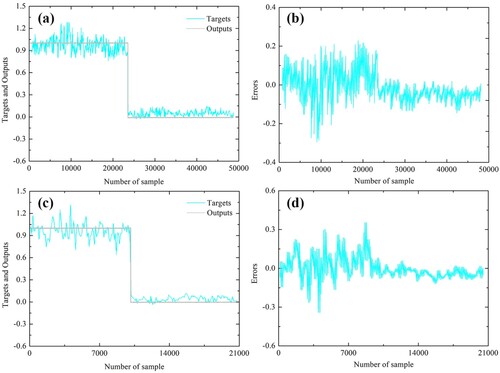
Figure 16. CNN model: (a) target and output values of training data samples, (b) magnitude of training error, (c) target and output values of validation data samples, and (d) magnitude of validation error.

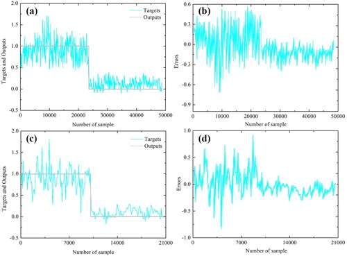
Figure 17. CNN-BWO model: (a) target and output values of training data samples, (b) magnitude of training error, (c) target and output values of validation data samples, and (d) magnitude of validation error.

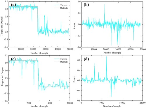
Figure 18. CNN-COA model: (a) target and output values of training data samples, (b) magnitude of training error, (c) target and output values of validation data samples, and (d) magnitude of validation error.

Overall, the enhanced efficiency of the metaheuristic optimization technique was consistent with earlier studies that combined the optimization algorithm and machine learning model (Balogun et al. 2021; Wang et al. 2021; Lv et al. 2022; Huang et al. 2023). In this work, the implementation of an optimization algorithm to be combined with the deep learning algorithm based on the CNN model provides a promising result, particularly when the COA optimization algorithm is used as the highest predictive model. As a result, in this study, the CNN-COA model is regarded as the optimum model for LSM. Nevertheless, among the countless models, it is difficult to find the optimal model for LSM in a particular geo-environment, and other hybrid models should be further investigated.

Although this study contributes to the research on landslide susceptibility mapping, there are still some limitations. First, in the different geomorphic units, not all slide and flow typologies could be predicted with the same precision. On the one hand, this is due to their high reliance on some factors not considered in the current assessment or on the interplay of local conditions. On the other hand, even the factors that were examined are likely to differ in how they regulate different types of movement. By increasing the typological specificity of the susceptibility assessments, this aspect can be better accounted for in the future. Second, nonlandslide points were randomly selected in a 1:1 ratio from landslide-free area. This selection method may have a negative impact on the evaluation results. Existing studies have demonstrated that different sampling ratios of nonlandslide points can greatly influence the original landslide susceptibility evaluation results (Hong et al. 2019; Chang et al. 2023; Liu, Tang, and Huang 2023). Therefore, to ensure the accuracy of the results of LSM, the optimized sampling ratio of nonlandslide locations should be given more consideration. Third, the landslide susceptibility analysis in the study area is stationary in time. This is not valid because landslide-inducing factors (such as rainfall and earthquakes) may vary over time. Furthermore, along with the occurrence of new landslides, the landslide inventory must also be updated. Therefore, multitemporal data on landslide conditioning variables and inventories should be gathered, and transfer learning may be a useful method for evaluating those temporal changes.

7. Conclusions

This study developed two innovative hybrid models for the spatially explicit prediction of landslide susceptibility by combining the CNN model with the BWO and COA optimization techniques. This is the first study to create such models and test their utility using actual, spatially explicit data from a landslide-prone region of Sichuan Province. Fourteen landslide conditioning factors were used to prepare the training datasets for the susceptibility analysis. The relative contribution of conditioning factors was assessed using the LSVM method. All fourteen factors are to some extent responsible for LSM and are thus used for spatial landslide modeling in Sichuan Province. The ROC curve, RMSE, and other statistical metrics were used to analyze the accuracy assessment and performance of the three models. The results revealed that there was satisfactory agreement between the predicted susceptibility grades and the known landslide locations using the two hybrid models. The results showed that the CNN-COA model had superior performance in LSM, with the highest AUC values of 0.946 and 0.919 for the training and validation datasets, respectively. Following this model for the training datasets were the CNN-BWO model and the CNN model (AUC values of 0.937 and 0.855, respectively), and for the validation datasets, the CNN-BWO model and the CNN model (AUC values of 0.906 and 0.805, respectively). The hybrid models used in this work greatly increase the CNN model's accuracy, showing that BWO and COA optimization techniques are promising approaches for LSM. The CNN-COA model generated the best landslide susceptibility map in terms of overall performance. As a result, the CNN-COA model was chosen as the best model for LSM in the study region. The mapping unit used in this study is the grid cell, which has little physical significance and cannot accurately represent the geological or geomorphological characteristics of natural slopes. Instead, the slope unit based on terrain segmentation can more accurately reflect the variables that influence the occurrence of landslides. Therefore, in future research, the slope unit should be used to analyze landslide susceptibility. In addition, a deeper and wider CNN architecture can be used to create a more accurate and robust hybrid model. Transfer learning can be investigated to optimize the parameters based on historical data from the local area, characterize local characteristics, and further improve the model's capacity for generalization and robustness when used across different geographical areas. Overall, the generated landslide susceptibility maps can be useful for better land use management and can help decision-makers provide a better approach to mitigate further loss in the case study area by providing a better prevention strategy in vulnerable areas.

Disclosure statement

No potential conflict of interest was reported by the author(s).

Data availability statement

The data or code used in this study are available from the corresponding author on reasonable request.

Additional information

Funding

This work was supported by China Postdoctoral Science Foundation: [grant number 2020M680583]; National Natural Science Foundation of China [grant number 52208359 ]; National Natural Science Foundation of China: [grant number 52109125]; National Postdoctoral Program for Innovative Talents: [grant number BX20200191].

References

- Abdollahzadeh, B., F. S. Gharehchopogh, N. Khodadadi, and S. Mirjalili. 2022. “Mountain Gazelle Optimizer: A New Nature-Inspired Metaheuristic Algorithm for Global Optimization Problems.” Advances in Engineering Software 174: 103282. https://doi.org/10.1016/j.advengsoft.2022.103282.
- Abdulwahid, W. M., and B. Pradhan. 2017. “Landslide Vulnerability and Risk Assessment for Multi-Hazard Scenarios Using Airborne Laser Scanning Data (LiDAR).” Landslides 14 (3): 1057–1076. https://doi.org/10.1007/s10346-016-0744-0.
- Abedini, M., B. Ghasemian, A. Shirzadi, H. Shahabi, K. Chapi, B. T. Pham, B. B. Ahmad, and D. Tien Bui. 2019. “A Novel Hybrid Approach of Bayesian Logistic Regression and Its Ensembles for Landslide Susceptibility Assessment.” Geocarto International 34 (13): 1427–1457. https://doi.org/10.1080/10106049.2018.1499820.
- Abedini, M., and S. Tulabi. 2018. “Assessing LNRF, FR, and AHP Models in Landslide Susceptibility Mapping Index: A Comparative Study of Nojian Watershed in Lorestan Province, Iran.” Environmental Earth Sciences 77 (11): 1–13. https://doi.org/10.1007/s12665-018-7524-1.
- Abualigah, L., M. Abd Elaziz, P. Sumari, Z. W. Geem, and A. H. Gandomi. 2022. “Reptile Search Algorithm (RSA): A Nature-Inspired Meta-Heuristic Optimizer.” Expert Systems with Applications 191: 116158. https://doi.org/10.1016/j.eswa.2021.116158.
- Al-Najjar, H. A., and B. Pradhan. 2021. “Spatial Landslide Susceptibility Assessment Using Machine Learning Techniques Assisted by Additional Data Created with Generative Adversarial Networks.” Geoscience Frontiers 12 (2): 625–637. https://doi.org/10.1016/j.gsf.2020.09.002.
- Alqadhi, S., J. Mallick, S. Talukdar, A. A. Bindajam, T. K. Saha, M. Ahmed, and R. A. Khan. 2021. “Combining Logistic Regression-Based Hybrid Optimized Machine Learning Algorithms with Sensitivity Analysis to Achieve Robust Landslide Susceptibility Mapping.” Geocarto International 37 (25): 9518–9543. https://doi.org/10.1080/10106049.2021.2022009.
- Aslam, B., A. Zafar, and U. Khalil. 2023. “Comparative Analysis of Multiple Conventional Neural Networks for Landslide Susceptibility Mapping.” Natural Hazards 115 (1): 673–707. https://doi.org/10.1007/s11069-022-05570-x.
- Azarafza, M., M. Azarafza, H. Akgün, P. M. Atkinson, and R. Derakhshani. 2021. “Deep Learning-Based Landslide Susceptibility Mapping.” Scientific Reports 11 (1): 24112. https://doi.org/10.1038/s41598-021-03585-1.
- Azarafza, M., A. Ghazifard, H. Akgün, and E. Asghari-Kaljahi. 2018. “Landslide Susceptibility Assessment of South Pars Special Zone, Southwest Iran.” Environmental Earth Sciences 77 (24): 1–29. https://doi.org/10.1007/s12665-018-7978-1.
- Balogun, A. L., F. Rezaie, Q. B. Pham, L. Gigović, S. Drobnjak, Y. A. Aina, M. Panahi, S. T. Yekeen, and S. Lee. 2021. “Spatial Prediction of Landslide Susceptibility in Western Serbia Using Hybrid Support Vector Regression (SVR) with GWO, BAT and COA Algorithms.” Geoscience Frontiers 12 (3): 101104. https://doi.org/10.1016/j.gsf.2020.10.009.
- Berhane, G., M. Kebede, and N. Alfarrah. 2021. “Landslide Susceptibility Mapping and Rock Slope Stability Assessment Using Frequency Ratio and Kinematic Analysis in the Mountains of Mgulat Area, Northern Ethiopia.” Bulletin of Engineering Geology and the Environment 80 (1): 285–301. https://doi.org/10.1007/s10064-020-01905-9.
- Bozzolan, E., E. A. Holcombe, F. Pianosi, I. Marchesini, M. Alvioli, and T. Wagener. 2023. “A Mechanistic Approach to Include Climate Change and Unplanned Urban Sprawl in Landslide Susceptibility Maps.” Science of the Total Environment 858: 159412. https://doi.org/10.1016/j.scitotenv.2022.159412.
- Brabb, E. E. 1984. “Innovative Approaches to Landslide Hazard Mapping.” Paper presented at proceedings 4th international symposium on landslides, Toronto, Canada, September 1984.
- Carrara, A., M. Cardinali, R. Detti, F. Guzzetti, V. Pasqui, and P. Reichenbach. 1991. “GIS Techniques and Statistical Models in Evaluating Landslide Hazard.” Earth Surface Processes and Landforms 16 (5): 427–445. https://doi.org/10.1002/esp.3290160505.
- Chang, Z., J. Huang, F. Huang, K. Bhuyan, S. R. Meena, and F. Catani. 2023. “Uncertainty Analysis of non-Landslide Sample Selection in Landslide Susceptibility Prediction Using Slope Unit-Based Machine Learning Models.” Gondwana Research 117: 307–320. https://doi.org/10.1016/j.gr.2023.02.007.
- Chen, Z., H. Zhou, F. Ye, B. Liu, and W. Fu. 2022. “Landslide Susceptibility Mapping Along the Anninghe Fault Zone in China Using SVM and ACO-PSO-SVM Models.” Lithosphere 2022 (1): 5216125. https://doi.org/10.2113/2022/5216125.
- Chou, J. S., and D. N. Truong. 2021. “A Novel Metaheuristic Optimizer Inspired by Behavior of Jellyfish in Ocean.” Applied Mathematics and Computation 389: 125535. https://doi.org/10.1016/j.amc.2020.125535.
- Dehghani, M., Z. Montazeri, E. Trojovská, and P. Trojovský. 2023. “Coati Optimization Algorithm: A new bio-Inspired Metaheuristic Algorithm for Solving Optimization Problems.” Knowledge-Based Systems 259: 110011. https://doi.org/10.1016/j.knosys.2022.110011.
- Dou, J., A. P. Yunus, D. T. Bui, A. Merghadi, M. Sahana, Z. Zhu, C. Chen, Z. Han, and B. T. Pham. 2020. “Improved Landslide Assessment Using Support Vector Machine with Bagging, Boosting, and Stacking Ensemble Machine Learning Framework in a Mountainous Watershed, Japan.” Landslides 17 (3): 641–658. https://doi.org/10.1007/s10346-019-01286-5.
- Eker, A. M., M. Dikmen, S. Cambazoğlu, H. S. B. Düzgün, and H. Akgün. 2012. “Application of Artificial Neural Network and Logistic Regression Methods to Landslide Susceptibility Mapping and Comparison of the Results for the Ulus District, Bartın.” Special issue, Journal of the Faculty of Engineering and Architecture of Gazi University 27 (1): 163–173.
- Eker, A. M., M. Dikmen, S. Cambazoğlu, ŞH Düzgün, and H. Akgün. 2015. “Evaluation and Comparison of Landslide Susceptibility Mapping Methods: A Case Study for the Ulus District, Bartın, Northern Turkey.” International Journal of Geographical Information Science 29 (1): 132–158. https://doi.org/10.1080/13658816.2014.953164.
- Fang, Z., Y. Wang, L. Peng, and H. Hong. 2021. “A Comparative Study of Heterogeneous Ensemble-Learning Techniques for Landslide Susceptibility Mapping.” International Journal of Geographical Information Science 35 (2): 321–347. https://doi.org/10.1080/13658816.2020.1808897.
- GAR (Global Assessment Report On Disaster Risk Reduction). 2009. Global Assessment Report on Disaster Risk Reduction. Geneva, Switzerland: United Nations International Strategy for Disaster Reduction Secretariat.
- GAR (Global Assessment Report On Disaster Risk Reduction). 2019. Global Assessment Report on Disaster Risk Reduction. Geneva, Switzerland: United Nations Office for Disaster Risk Reduction.
- Ghorbanzadeh, O., K. Gholamnia, and P. Ghamisi. 2022. “The Application of ResU-net and OBIA for Landslide Detection from Multi-Temporal Sentinel-2 Images.” Big Earth Data, 1–26. https://doi.org/10.1080/20964471.2022.2031544.
- Guo, Z., Y. Shi, F. Huang, X. Fan, and J. Huang. 2021. “Landslide Susceptibility Zonation Method Based on C5. 0 Decision Tree and K-Means Cluster Algorithms to Improve the Efficiency of Risk Management.” Geoscience Frontiers 12 (6): 101249. https://doi.org/10.1016/j.gsf.2021.101249.
- Guzzetti, F., A. Carrara, M. Cardinali, and P. Reichenbach. 1999. “Landslide Hazard Evaluation: A Review of Current Techniques and Their Application in a Multi-Scale Study, Central Italy.” Geomorphology 31 (1-4): 181–216. https://doi.org/10.1016/S0169-555X(99)00078-1.
- Hodasová, K., and M. Bednarik. 2021. “Effect of Using Various Weighting Methods in a Process of Landslide Susceptibility Assessment.” Natural Hazards 105 (1): 481–499. https://doi.org/10.1007/s11069-020-04320-1.
- Hong, H., Y. Miao, J. Liu, and A. X. Zhu. 2019. ““Exploring the Effects of the Design and Quantity of Absence Data on the Performance of Random Forest-Based Landslide Susceptibility Mapping.”.” Catena 176: 45–64. https://doi.org/10.1016/j.catena.2018.12.035.
- Houssein, E. H., D. Oliva, E. Çelik, M. M. Emam, and R. M. Ghoniem. 2023. “Boosted Sooty Tern Optimization Algorithm for Global Optimization and Feature Selection.” Expert Systems with Applications 213: 119015. https://doi.org/10.1016/j.eswa.2022.119015.
- Hu, Q., Y. Zhou, S. Wang, and F. Wang. 2020. “Machine Learning and Fractal Theory Models for Landslide Susceptibility Mapping: Case Study from the Jinsha River Basin.” Geomorphology 351: 106975. https://doi.org/10.1016/j.geomorph.2019.106975.
- Huang, F., Z. Cao, J. Guo, S. H. Jiang, S. Li, and Z. Guo. 2020. “Comparisons of Heuristic, General Statistical and Machine Learning Models for Landslide Susceptibility Prediction and Mapping.” Catena 191: 104580. https://doi.org/10.1016/j.catena.2020.104580.
- Huang, F., J. Chen, W. Liu, J. Huang, H. Hong, and W. Chen. 2022. “Regional Rainfall-Induced Landslide Hazard Warning Based on Landslide Susceptibility Mapping and a Critical Rainfall Threshold.” Geomorphology 408: 108236. https://doi.org/10.1016/j.geomorph.2022.108236.
- Huang, W., M. Ding, Z. Li, J. Yu, D. Ge, Q. Liu, and J. Yang. 2023. “Landslide Susceptibility Mapping and Dynamic Response Along the Sichuan-Tibet Transportation Corridor Using Deep Learning Algorithms.” Catena 222: 106866. https://doi.org/10.1016/j.catena.2022.106866.
- Huang, F., Z. Ye, S. Jiang, J. Huang, Z. Chang, and J. Chen. 2021. “Uncertainty Study of Landslide Susceptibility Prediction Considering the Different Attribute Interval Numbers of Environmental Factors and Different Data-Based Models.” Catena 202: 105250. https://doi.org/10.1016/j.catena.2021.105250.
- Hung, L. Q., N. T. H. Van, P. Van Son, N. H. Khanh, and L. T. Binh. 2016. “Landslide Susceptibility Mapping by Combining the Analytical Hierarchy Process and Weighted Linear Combination Methods: A Case Study in the Upper Lo River Catchment (Vietnam).” Landslides 13 (5): 1285–1301. https://doi.org/10.1007/s10346-015-0657-3.
- Jaafari, A., M. Panahi, D. Mafi-Gholami, O. Rahmati, H. Shahabi, A. Shirzadi, S. Lee, D. T. Bui, and B. Pradhan. 2022. “Swarm Intelligence Optimization of the Group Method of Data Handling Using the Cuckoo Search and Whale Optimization Algorithms to Model and Predict Landslides.” Applied Soft Computing 116: 108254. https://doi.org/10.1016/j.asoc.2021.108254.
- Jafari, M., E. Salajegheh, and J. Salajegheh. 2021. “Elephant Clan Optimization: A Nature-Inspired Metaheuristic Algorithm for the Optimal Design of Structures.” Applied Soft Computing 113: 107892. https://doi.org/10.1016/j.asoc.2021.107892.
- Ji, J., H. Cui, T. Zhang, J. Song, and Y. Gao. 2022. “A GIS-Based Tool for Probabilistic Physical Modelling and Prediction of Landslides: GIS-FORM Landslide Susceptibility Analysis in Seismic Areas.” Landslides 19 (9): 2213–2231. https://doi.org/10.1007/s10346-022-01885-9.
- Jiao, Y., D. Zhao, Y. Ding, Y. Liu, Q. Xu, Y. Qiu, C. Liu, Z. Liu, Z. Zha, and R. Li. 2019. “Performance Evaluation for Four GIS-Based Models Purposed to Predict and map Landslide Susceptibility: A Case Study at a World Heritage Site in Southwest China.” Catena 183: 104221. https://doi.org/10.1016/j.catena.2019.104221.
- Kim, H. G., D. K. Lee, C. Park, Y. Ahn, S. H. Kil, S. Sung, and G. S. Biging. 2018. “Estimating Landslide Susceptibility Areas Considering the Uncertainty Inherent in Modeling Methods.” Stochastic Environmental Research and Risk Assessment 32 (11): 2987–3019. https://doi.org/10.1007/s00477-018-1609-y.
- Kornejady, A., M. Ownegh, and A. Bahremand. 2017. “Landslide Susceptibility Assessment Using Maximum Entropy Model with two Different Data Sampling Methods.” Catena 152: 144–162. https://doi.org/10.1016/j.catena.2017.01.010.
- Kuyu, YÇ, and F. Vatansever. 2022. “GOZDE: A Novel Metaheuristic Algorithm for Global Optimization.” Future Generation Computer Systems 136: 128–152. https://doi.org/10.1016/j.future.2022.05.022.
- Li, Y., W. Wang, G. Wang, and Q. Tan. 2022. “Actual Evapotranspiration Estimation Over the Tuojiang River Basin Based on a Hybrid CNN-RF Model.” Journal of Hydrology 610: 127788. https://doi.org/10.1016/j.jhydrol.2022.127788.
- Lin, Q., S. Steger, M. Pittore, J. Zhang, L. Wang, T. Jiang, and Y. Wang. 2022. “Evaluation of Potential Changes in Landslide Susceptibility and Landslide Occurrence Frequency in China Under Climate Change.” Science of the Total Environment 850: 158049. https://doi.org/10.1016/j.scitotenv.2022.158049.
- Liu, Q., A. Tang, and D. Huang. 2023. “Exploring the Uncertainty of Landslide Susceptibility Assessment Caused by the Number of Non–Landslides.” Catena 227: 107109. https://doi.org/10.1016/j.catena.2023.107109.
- Lucchese, L. V., G. G. de Oliveira, and O. C. Pedrollo. 2021. “Investigation of the Influence of Nonoccurrence Sampling on Landslide Susceptibility Assessment Using Artificial Neural Networks.” Catena 198: 105067. https://doi.org/10.1016/j.catena.2020.105067.
- Lv, L., T. Chen, J. Dou, and A. Plaza. 2022. “A Hybrid Ensemble-Based Deep-Learning Framework for Landslide Susceptibility Mapping.” International Journal of Applied Earth Observation and Geoinformation 108: 102713. https://doi.org/10.1016/j.jag.2022.102713.
- Mandal, K., S. Saha, and S. Mandal. 2021. “Applying Deep Learning and Benchmark Machine Learning Algorithms for Landslide Susceptibility Modelling in Rorachu River Basin of Sikkim Himalaya, India.” Geoscience Frontiers 12 (5): 101203. https://doi.org/10.1016/j.gsf.2021.101203.
- Mebrahtu, T. K., T. Heinze, S. Wohnlich, and M. Alber. 2022. “Slope Stability Analysis of Deep-Seated Landslides Using Limit Equilibrium and Finite Element Methods in Debre Sina Area, Ethiopia.” Bulletin of Engineering Geology and the Environment 81 (10): 403. https://doi.org/10.1007/s10064-022-02906-6.
- Merghadi, A., A. P. Yunus, J. Dou, J. Whiteley, B. ThaiPham, D. T. Bui, R. Avtar, and B. Abderrahmane. 2020. “Machine Learning Methods for Landslide Susceptibility Studies: A Comparative Overview of Algorithm Performance.” Earth-Science Reviews 207: 103225. https://doi.org/10.1016/j.earscirev.2020.103225.
- Momeny, M., A. A. Neshat, A. Gholizadeh, A. Jafarnezhad, E. Rahmanzadeh, M. Marhamati, B. Moradi, A. Ghafoorifar, and Y. D. Zhang. 2022. “Greedy Autoaugment for Classification of Mycobacterium Tuberculosis Image via Generalized Deep CNN Using Mixed Pooling Based on Minimum Square Rough Entropy.” Computers in Biology and Medicine 141: 105175. https://doi.org/10.1016/j.compbiomed.2021.105175.
- Ngo, P. T. T., M. Panahi, K. Khosravi, O. Ghorbanzadeh, N. Kariminejad, A. Cerda, and S. Lee. 2021. “Evaluation of Deep Learning Algorithms for National Scale Landslide Susceptibility Mapping of Iran.” Geoscience Frontiers 12 (2): 505–519. https://doi.org/10.1016/j.gsf.2020.06.013.
- Nikoobakht, S., M. Azarafza, H. Akgün, and R. Derakhshani. 2022. “Landslide Susceptibility Assessment by Using Convolutional Neural Network.” Applied Sciences 12 (12): 1–22. https://doi.org/10.3390/app12125992.
- Okalp, K., and H. Akgün. 2016. “National Level Landslide Susceptibility Assessment of Turkey Utilizing Public Domain Dataset.” Environmental Earth Sciences 75 (9): 1–21. https://doi.org/10.1007/s12665-016-5640-3.
- Okalp, K., and H. Akgün. 2022. “Landslide Susceptibility Assessment in Medium-Scale: Case Studies from the Major Drainage Basins of Turkey.” Environmental Earth Sciences 81 (8): 244. https://doi.org/10.1007/s12665-022-10355-3.
- Ozturk, D., and N. Uzel-Gunini. 2022. “Investigation of the Effects of Hybrid Modeling Approaches, Factor Standardization, and Categorical Mapping on the Performance of Landslide Susceptibility Mapping in Van, Turkey.” Natural Hazards 114 (3): 2571–2604. https://doi.org/10.1007/s11069-022-05480-y.
- Petley, D. 2012. “Global Patterns of Loss of Life from Landslides.” Geology 40 (10): 927–930. https://doi.org/10.1130/G33217.1.
- Pham, B. T., I. Prakash, and D. T. Bui. 2018. “Spatial Prediction of Landslides Using a Hybrid Machine Learning Approach Based on Random Subspace and Classification and Regression Trees.” Geomorphology 303: 256–270. https://doi.org/10.1016/j.geomorph.2017.12.008.
- Pham, B. T., D. Tien Bui, H. R. Pourghasemi, P. Indra, and M. B. Dholakia. 2017. “Landslide Susceptibility Assesssment in the Uttarakhand Area (India) Using GIS: A Comparison Study of Prediction Capability of Naïve Bayes, Multilayer Perceptron Neural Networks, and Functional Trees Methods.” Theoretical and Applied Climatology 128 (1-2): 255–273. https://doi.org/10.1007/s00704-015-1702-9.
- Pourghasemi, H. R., and O. Rahmati. 2018. “Prediction of the Landslide Susceptibility: Which Algorithm, Which Precision?” Catena 162: 177–192. https://doi.org/10.1016/j.catena.2017.11.022.
- Reichenbach, P., M. Rossi, B. D. Malamud, M. Mihir, and F. Guzzetti. 2018. “A Review of Statistically-Based Landslide Susceptibility Models.” Earth-Science Reviews 180: 60–91. https://doi.org/10.1016/j.earscirev.2018.03.001.
- Roy, P., S. C. Pal, R. Chakrabortty, I. Chowdhuri, S. Malik, and B. Das. 2020. “Threats of Climate and Land Use Change on Future Flood Susceptibility.” Journal of Cleaner Production 272: 122757. https://doi.org/10.1016/j.jclepro.2020.122757.
- Sameen, M. I., B. Pradhan, and S. Lee. 2020. “Application of Convolutional Neural Networks Featuring Bayesian Optimization for Landslide Susceptibility Assessment.” Catena 186: 104249. https://doi.org/10.1016/j.catena.2019.104249.
- Schuster, Robert L. 1996. “Socioeconomic Significance of Landslides.” In Landslides: Investigation and Mitigation, Transportation Research Board Special Report 247, edited by A. K. Turner, and R. L. Schuster, 12–35. Washington, DC, USA: National Academy of Sciences.
- Shirani, K., M. Pasandi, and A. Arabameri. 2018. “Landslide Susceptibility Assessment by Dempster–Shafer and Index of Entropy Models, Sarkhoun Basin, Southwestern Iran.” Natural Hazards 93 (3): 1379–1418. https://doi.org/10.1007/s11069-018-3356-2.
- Sun, D., S. Shi, H. Wen, J. Xu, X. Zhou, and J. Wu. 2021. “A Hybrid Optimization Method of Factor Screening Predicated on GeoDetector and Random Forest for Landslide Susceptibility Mapping.” Geomorphology 379: 107623. https://doi.org/10.1016/j.geomorph.2021.10762.
- Taalab, K., T. Cheng, and Y. Zhang. 2018. “Mapping Landslide Susceptibility and Types Using Random Forest.” Big Earth Data 2 (2): 159–178. https://doi.org/10.1080/20964471.2018.1472392.
- Tien Bui, D., T. A. Tuan, H. Klempe, B. Pradhan, and I. Revhaug. 2016. “Spatial Prediction Models for Shallow Landslide Hazards: A Comparative Assessment of the Efficacy of Support Vector Machines, Artificial Neural Networks, Kernel Logistic Regression, and Logistic Model Tree.” Landslides 13 (2): 361–378. https://doi.org/10.1007/s10346-015-0557-6.
- Trinh, T., B. T. Luu, T. H. T. Le, D. H. Nguyen, T. Van Tran, T. H. Van Nguyen, K. Q. Nguye, and L. T. Nguyen. 2022. “A Comparative Analysis of Weight-Based Machine Learning Methods for Landslide Susceptibility Mapping in Ha Giang Area.” Big Earth Data, 1–30. https://doi.org/10.1080/20964471.2022.2043520.
- Ullah, K., Y. Wang, Z. Fang, L. Wang, and M. Rahman. 2022. “Multi-hazard Susceptibility Mapping Based on Convolutional Neural Networks.” Geoscience Frontiers 13 (5): 101425. https://doi.org/10.1016/j.gsf.2022.101425.
- Wang, Y., Z. Fang, and H. Hong. 2019. “Comparison of Convolutional Neural Networks for Landslide Susceptibility Mapping in Yanshan County, China.” Science of the Total Environment 666: 975–993. https://doi.org/10.1016/j.scitotenv.2019.02.263.
- Wang, Y., L. Feng, S. Li, F. Ren, and Q. Du. 2020. “A Hybrid Model Considering Spatial Heterogeneity for Landslide Susceptibility Mapping in Zhejiang Province, China.” Catena 188: 104425. https://doi.org/10.1016/j.catena.2019.104425.
- Wang, H., L. Zhang, H. Luo, J. He, and R. W. M. Cheung. 2021. “AI-powered Landslide Susceptibility Assessment in Hong Kong.” Engineering Geology 288: 106103. https://doi.org/10.1016/j.enggeo.2021.106103.
- Wei, X., L. Zhang, P. Gardoni, Y. Chen, L. Tan, D. Liu, C. Du, and H. Li. 2023. “Comparison of Hybrid Data-Driven and Physical Models for Landslide Susceptibility Mapping at Regional Scales.” Acta Geotechnica, 1–24. https://doi.org/10.1007/s11440-023-01841-4.
- Wu, Y., Y. Ke, Z. Chen, S. Liang, H. Zhao, and H. Hong. 2020. “Application of Alternating Decision Tree with AdaBoost and Bagging Ensembles for Landslide Susceptibility Mapping.” Catena 187: 104396. https://doi.org/10.1016/j.catena.2019.104396.
- Xie, Y., W. Sun, M. Ren, S. Chen, Z. Huang, and X. Pan. 2023. “Stacking Ensemble Learning Models for Daily Runoff Prediction Using 1D and 2D CNNs.” Expert Systems with Applications 217: 119469. https://doi.org/10.1016/j.eswa.2022.119469.
- Yang, Z., J. Li, J. Hyyppä, J. Gong, J. Liu, and B. Yang. 2023. “A Comprehensive and up-to-Date Web-Based Interactive 3D Emergency Response and Visualization System Using Cesium Digital Earth: Taking Landslide Disaster as an Example.” Big Earth Data, 1–23. https://doi.org/10.1080/20964471.2023.2172823.
- Yi, Y., Z. Zhang, W. Zhang, Q. Xu, C. Deng, and Q. Li. 2019. “GIS-based Earthquake-Triggered-Landslide Susceptibility Mapping with an Integrated Weighted Index Model in Jiuzhaigou Region of Sichuan Province, China.” Natural Hazards and Earth System Sciences 19 (9): 1973–1988. https://doi.org/10.5194/nhess-19-1973-2019.
- Yin, G., J. Luo, F. Niu, Z. Lin, and M. Liu. 2021. “Machine Learning-Based Thermokarst Landslide Susceptibility Modeling Across the Permafrost Region on the Qinghai-Tibet Plateau.” Landslides 18 (7): 2639–2649. https://doi.org/10.1007/s10346-021-01669-7.
- Youssef, A. M., and H. R. Pourghasemi. 2021. “Landslide Susceptibility Mapping Using Machine Learning Algorithms and Comparison of Their Performance at Abha Basin, Asir Region, Saudi Arabia.” Geoscience Frontiers 12 (2): 639–655. https://doi.org/10.1016/j.gsf.2020.05.010.
- Youssef, A. M., B. Pradhan, A. Dikshit, M. M. Al-Katheri, S. S. Matar, and A. M. Mahdi. 2022. “Landslide Susceptibility Mapping Using CNN-1D and 2D Deep Learning Algorithms: Comparison of Their Performance at Asir Region, KSA.” Bulletin of Engineering Geology and the Environment 81 (4): 165. https://doi.org/10.1007/s10064-022-02657-4.
- Zhang, J., X. Ma, J. Zhang, D. Sun, X. Zhou, C. Mi, and H. Wen. 2023. “Insights Into Geospatial Heterogeneity of Landslide Susceptibility Based on the SHAP-XGBoost Model.” Journal of Environmental Management 332: 117357. https://doi.org/10.1016/j.jenvman.2023.117357.
- Zhao, Z., and J. Chen. 2023. “A Robust Discretization Method of Factor Screening for Landslide Susceptibility Mapping Using Convolution Neural Network, Random Forest, and Logistic Regression Models.” International Journal of Digital Earth 16 (1): 408–429. https://doi.org/10.1080/17538947.2023.2174192.
- Zhong, C., G. Li, and Z. Meng. 2022. “Beluga Whale Optimization: A Novel Nature-Inspired Metaheuristic Algorithm.” Knowledge-Based Systems 251: 109215. https://doi.org/10.1016/j.knosys.2022.109215.
- Zhou, X., H. Wen, Y. Zhang, J. Xu, and W. Zhang. 2021. “Landslide Susceptibility Mapping Using Hybrid Random Forest with GeoDetector and RFE for Factor Optimization.” Geoscience Frontiers 12 (5): 101211. https://doi.org/10.1016/j.gsf.2021.101211.