Spectral clustering eigenvector selection of hyperspectral image based on the coincidence degree of data distribution

ABSTRACT

Spectral clustering is a well-regarded subspace clustering algorithm that exhibits outstanding performance in hyperspectral image classification through eigenvalue decomposition of the Laplacian matrix. However, its classification accuracy is severely limited by the selected eigenvectors, and the commonly used eigenvectors not only fail to guarantee the inclusion of detailed discriminative information, but also have high computational complexity. To address these challenges, we proposed an intuitive eigenvector selection method based on the coincidence degree of data distribution (CDES). First, the clustering result of improved k-means, which can well reflect the spatial distribution of various types was used as the reference map. Then, the adjusted Rand index and adjusted mutual information were calculated to assess the data distribution consistency between each eigenvector and the reference map. Finally, the eigenvectors with high coincidence degrees were selected for clustering. A case study on hyperspectral mineral mapping demonstrated that the mapping accuracies of CDES are approximately 56.3%, 15.5%, and 10.5% higher than those of the commonly used top, high entropy, and high relevance eigenvectors, and CDES can save more than 99% of the eigenvector selection time. Especially, due to the unsupervised nature of k-means, CDES provides a novel solution for autonomous feature selection of hyperspectral images.

KEYWORDS:

• Eigenvector selection
• spectral clustering
• coincidence degree of data distribution
• hyperspectral mineral mapping

1. Introduction

Clustering is a powerful technique in several advanced data analysis tasks such as pattern recognition, data mining, and image classification (Filippone et al. 2008). The purpose of clustering is to partition a dataset into several expected clusters, so that the data points in the same cluster are similar to each other but dissimilar from the data points of other clusters. As an unsupervised algorithm, clustering can avoid the tedious and often inconsistent manual data labeling process. This makes it play a crucial role in processing hyperspectral remote sensing images, where labeled samples are laborious to produce or are often inadequate.

Hyperspectral image (HSI) consists of hundreds of contiguous bands covering the spectral range from the visible to shortwave infrared spectra. Rich spectral information provides detailed discriminative features and makes HSI a powerful tool in the accurate identification of fine objects such as minerals and vegetation. However, the curse of dimensionality seriously affects the classification accuracy and efficiency of HSIs (Li et al. 2022). Moreover, the presence of nonlinear media, subpixel heterogeneity, and multiple scattering render HSI to have a nonlinear structure (Bachmann, Ainsworth, and Fusina 2005), which introduces several complexities that can be problematic with conventional clustering algorithms (Hassanzadeh, Kaarna, and Kauranne 2018). To mitigate these problems, a useful extension of conventional clustering is the application of dimensionality reduction techniques, namely subspace clustering (Liu, Jiao, and Shang 2013).

Spectral clustering is a widely used subspace clustering algorithm that has been successfully applied to HSI classification because of its efficiency in extracting the clusters with different geometric structures (Zhang et al. 2016). Generally, spectral clustering includes two steps: (1) reducing the dimensionality of the high-dimensional data by eigenvalue decomposition of the normalized Laplacian matrix; (2) selecting several eigenvectors for conventional clustering. In particular, eigenvector selection is critical for spectral clustering because uninformative eigenvectors could lead to poor clustering results (Toussi and Yazdi 2011). Currently, HSI classification studies based on spectral clustering typically use the top $M$ eigenvectors (TES) corresponding with the $M$ smallest eigenvalues of the normalized Laplacian matrix for data partitioning (Wang, Nie, and Yu 2017). However, it is not guaranteed that the top eigenvectors are equally informative even in an ‘ideal’ case (Prakash, Balasubramanian, and Sarma 2013), which means that some top eigenvectors may not contain strong discriminative information for clustering, thus losing the spatial distribution of certain types.

In fact, the eigenvector selection of spectral clustering can be divided into two critical issues: (1) How to put informative eigenvectors in the first place? (2) How to automatically determine the $\mathrm{M}$value (i.e. the number of eigenvectors) used for clustering? Aiming at these two issues, Xiang and Gong, who are the first to use eigenvector selection to improve the spectral clustering results, think that the key is to select relevant eigenvectors that provide useful information about the natural grouping of data (Xiang and Gong 2008). Therefore, they first calculated the relevance of each eigenvector, and then the eigenvectors with relevant values greater than 0.5 were selected for spectral clustering. Eigenvectors with high relevance (RES) exhibit promising performance in image segmentation. Entropy theory is another popular approach for eigenvector selection, and the eigenvectors with high entropy (EES) are typically selected for classification. For instance, Zhao et al. first computed entropy by substituting probability with similarity and then used the entropy to evaluate the importance of each eigenvector for clustering (Zhao et al. 2010). When the number of clusters ($\mathrm{K}$) is not large, 10 eigenvectors with greater importance were selected for clustering. The experiments showed that this eigenvector selection method performs slightly better than TES in spectral clustering. However, the huge computational complexity of RES and EES poses great challenge to their applications in large-scale datasets. More importantly, relevance and entropy are abstract and cannot intuitively reveal the original data structure. That is, like TES, there is no guarantee that the eigenvectors with high relevance or high entropy will contain detailed discriminative information for clustering. As for the determination of the $M$ value, the setting of 0.5 and 10 is somewhat arbitrary without strict theoretical basis.

Actually, the purpose of eigenvector selection is to find the features that can reveal the differences between various types so as to improve the HSI classification accuracies. From this point of view, an intuitive eigenvector selection approach is to first determine a reference map that can well reveal the differences between various types, and then the eigenvectors that match the data distribution of this reference map are highly likely to carry strong discriminative information for clustering. In this way, the eigenvector selection of spectral clustering can be transformed into the acquisition of the reference map and the calculation of data distribution consistency.

Ideally, the ground truth map should be used as the reference map. However, in practical application, the ground truth map is almost never available. Fortunately, Ren et al. have revealed that the clustering result of improved k-means, which uses spectral angle mapper (SAM) for clustering, can well reflect the spatial distribution of various types (Ren, Sun, and Zhai 2020). Because compared with Euclidean distance, cosine similarity is insensitive to the length of the spectral vector. Therefore, in this study, the clustering result of improved k-means was used as the reference map. Furthermore, since k-means is a fast unsupervised classification method, using the clustering result of improved k-means as the reference map can not only eliminate the dependence of eigenvector selection on the ground truth map, but also exhibit considerable potential for improving the eigenvector selection efficiency of large-scale datasets. In addition, two external clustering indexes, including the adjusted Rand index (ARI) and adjusted mutual information (AMI) can be used to find the eigenvectors that are highly consistent with the data distribution of the reference map. Because from a broad perspective, both ARI and AMI can measure the coincidence degree of two data distributions (Cao, Yomo, and Ying 2020).

In this study, hyperspectral mineral mapping was used to evaluate the performance of various eigenvector selection methods in spectral clustering of large-scale datasets. Furthermore, since the clustering result of spectral clustering only reflects the spatial distribution of various clusters without giving specific mineral types, the clustering-matching mapping method (Ren, Zhai, and Sun 2022), which matches the cluster centers with a spectral library, was used to obtain the final mineral mapping results. To the best of our knowledge, this study is the first to use eigenvector selection to improve the HSI classification results of spectral clustering, which will enhance the application of spectral clustering in hyperspectral data such as PRISMA and EnMap, and consequently the need to quickly process HSI.

2. Materials

2.1. Study area

The study area, Cuprite (Figure 1(a)), is a widely used alteration mineral area in Nevada, USA, and the alteration of Cuprite is related to the relict hydrothermal system (Chen, Warner, and Campagna 2007). Cuprite has been used as a geologic remote sensing test site since the early 1980s, because various mineral types in this area are exposed to very little vegetation cover (Resmini et al. 2010). Figure 1(b) exhibits the mineral distribution map of Cuprite derived from the United States Geological Survey (USGS). This distribution map was developed based on the vibrational absorption features of minerals and has been extensively field checked (Clark et al. 2003; Ni, Xu, and Zhou 2020). Six mineral types including alunite, kaolinite, calcite, chalcedony, muscovite, and montmorillonite have been discovered in this area.

Figure 1. Study area and hyperspectral data. (a) location map; (b) mineral distribution map; (c) AVIRIS image.

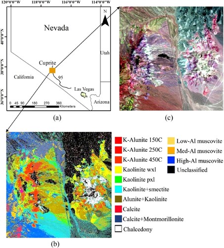
2.2. Hyperspectral data

The hyperspectral data was derived from airborne visible/infrared imaging spectrometer (AVIRIS), which has 224 spectral bands covering a spectral range of 0.4–2.5 µm. The AVIRIS image (Figure 1(c)) used in this study has 50 bands covering the shortwave infrared of 2.0–2.5 µm with a spatial resolution of 20 m and a spectral resolution of 10 nm, consisting of 350 lines and columns. This HSI was chosen because the spectral bands of 2.0–2.5 µm cover the spectral absorption features of many common minerals (Kruse, Boardman, and Huntington 2003). Moreover, this AVIRIS image has been processed by the atmosphere removal program (ATREM) and empirical flat field optimized reflectance transformation (EFFORT), which is essential for the clustering-matching mapping method and improved k-means. In addition, registration between the AVIRIS image and the mineral distribution map has been carried out to assess the mineral mapping accuracy.

3. Methodology

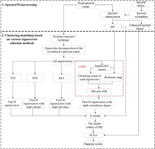
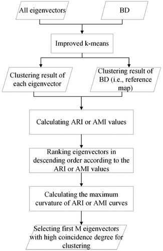
Figure 2 shows a flowchart of the clustering-matching mapping procedure of spectral clustering based on various eigenvector selection methods. In general, this procedure mainly includes four steps: (1) calculating the eigenvectors of the normalized Laplacian matrix; (2) selecting $M$ eigenvectors for clustering using various eigenvector selection methods, in which CDES represents the eigenvector selection method based on the coincidence degree of data distribution; (3) performing k-means clustering on the selected eigenvectors; (4) matching the cluster centers of band depth (BD) with the USGS mineral spectral library (Clark et al. 1993) using a combined spectral matching technique (SCGA) (Ren, Zhai, and Sun 2022). It should be noted that there are two k-means clustering processes in this clustering-matching mapping procedure. The first k-means (i.e. the improved k-means) in step 2 was used to obtain the reference map, and the second k-means in step 3 was used to obtain the spectral clustering results.

Figure 2. Flowchart of the clustering-matching mapping procedure of spectral clustering based on various eigenvector selection methods.

3.1. Spectral preprocessing

As clustering-matching requires the HSI and spectral library to have the same spectral range and resolution, spectral resampling of the USGS mineral spectral library was performed before matching. Furthermore, to enhance the spectral absorption features of various mineral types, band depth (BD) was calculated according to the following three steps (Noomen et al. 2006): (1) connecting the extreme points of the spectral curve to form the envelope; (2) dividing the original spectrum by the envelope to generate the continuum removal (CR); (3) subtracting CR from 1 to obtain BD. (1) $SL={\displaystyle \frac{R_e-R_s}{{\lambda }_e-{\lambda }_s}}$(1) (2) $CR={\displaystyle \frac{R_d}{R_s+SL\cdot ({\lambda }_d-{\lambda }_s)}}$(2)

(3) $BD=1-CR$(3)

Where $R$ is the reflectance; $\lambda$ is the wavelength; $SL$ represents the slope; $d$ is the band index; $e$ and $s$ are the ending and starting points of the segmented straight lines of the envelope, respectively.

3.2. Spectral clustering

Spectral clustering is a widely used graph-based clustering approach. It treats the HSI as an undirected graph and clusters data points by minimizing the connection weights between different clusters (Zhou et al. 2014). Specifically, given a dataset $X=\{x_1,x_2,\dots ,x_i,\dots ,x_N\}$, we can build a weighted undirected graph $G(X,E)$, in which $x_i$ denotes one row vector and contains $B$ elements; $N$ is the number of data points; and $E$ represents the set of edges. Each edge between two data points $x_i$ and $x_j$ carries a non-negative weight $w_{ij}$. The weights between all points form an $N\times N$ affinity matrix $W=(w_{ij}{)}_{i,j=1,\dots ,N}$. Each element in $W$ can be defined by a typical Gaussian function. (4) $w_{ij}=\{\begin{array}{c}\exp \left(-{\displaystyle \frac{x_i-x_j^2}{2{\sigma }^2}}\right),i\ne j\\ 0,i=j\end{array}$(4) where the parameter $\sigma$ controls the width of the neighborhoods and is set to 1 in this study. Let $D\in R^{N\times N}$ be the degree matrix whose diagonal element $d_i$($d_i=\sum _{j=1}^N{w}_{ij}$) is the column sum of the affinity matrix. Thus, the detailed algorithm steps of spectral clustering can be given as follows.

1. Form the $N\times N$ affinity matrix $W$ and the degree matrix $D$.

2. Compute the normalized Laplacian matrix $L=I-D^{-1/2}W{D}^{-1/2}$, where I is the $N\ast N$ identity matrix.

3. Calculate the top $M$ eigenvectors $v^1,v^2,\dots ,v^M$ of $L$, and then form the eigenvector matrix $V=[v^1,v^2,\dots ,v^M]\in R^{N\times M}$.

4. Form the matrix $Y$ by renormalizing each row of $V$ such that all rows in $Y$ have unit length, namely $Y_{ij}=V_{ij}/{\left(\sum _j{V}_{ij}^2\right)}^{1/2}$.

5. Cluster each row in $Y$ via k-means to obtain the final clustering result.

K-means is an iterative clustering algorithm. Its objective function is to minimize the sum of the squared errors (SSE) (Likas, Vlassis, and Verbeek 2003). (5) $SSE(C)=\sum _{i=1}^K\sum _{j=1}^{N_i}{q}_{ij}-c_i{F}^2$(5) where $||\cdot |{|}_F$ denotes the Frobenius norm; $c_i$ is one cluster center; $N_i$ is the data point number of $c_i$; $q_{ij}$ is one data point of $c_i$. Conventional k-means includes four steps: (1) initializing the $K$ value and cluster centers. For the first k-means, $K$ is set to 7, which includes six mineral types and the unclassified background type. For the second k-means, $K$ is set to 100, because a larger $K$ is conducive to improving the clustering-matching mapping accuracy (Ren, Sun, and Zhai 2020). The initial cluster centers are typically randomly selected from HSIs; (2) dividing the data points into the nearest cluster centers according to the Euclidean distance between pixels and cluster centers; (3) updating the cluster centers by calculating the average pixel values; and (4) going back to step 2 until the cluster centers do not change. The pseudocode for k-means is shown in Algorithm 1.

Algorithm 1: k-means

Input: Dataset $X=\{x_i{\}}_{i=1}^N$, number of clusters $K$

Output: Cluster assignments $\{{\delta }_{ij}{\}}_{i=1,\dots ,N,j=1,\dots ,K}$

1: Select $K$ data points randomly from $X$ as the initial cluster centers $c=\{c_1,\dots ,c_K\}$

2: While 1 do

3:  for i = 1 to $N$ do

4:   for j = 1 to $K$ do

5:    $d_i=x_i-c_j{F}^2$

6:   end for

7:   ${\delta }_{ij}=argmin(d_i)$

8:  end for

9:  Update cluster centers $c_i={\displaystyle \frac{1}{K_i}\sum _{j=1}^{K_i}{c}_{ij}}$

10:  if $c$ is stabilized then return $\{{\delta }_{ij}{\}}_{i=1,\dots ,N,j=1,\dots ,K}$

11:  else go back to step 3

12:  end if

13: End

Although spectral clustering does not require strong assumptions in the form of data points, its $O(N^2)$ space complexity and $O(N^3)$ time complexity are unacceptable when processing large-scale datasets (Jia, Ding, and Du 2017 ). Therefore, the Nyström extension technique (Fowlkes et al. 2004), which is one of the most popular methods for approximate spectral decomposition of a large kernel matrix, was used to calculate the approximate affinity matrix by randomly sampling 700 data points from the AVIRIS image.

3.3. Eigenvector selection

In this paper, four methods, including TES, RES, EES, and CDES, were used for the eigenvector selection of spectral clustering. In particular, considering that the pixel value of the eigenvector is a decimal, it is not easy to get the probability of each point; thus we compute the entropy of each eigenvector by substituting probability with similarity, and the specific calculation formula can be referred to (Zhao et al. 2010).

3.3.1. Acquisition of the reference map

In this study, the improved k-means uses spectral angle mapper (SAM) instead of Euclidean distance to calculate the similarity between various data points. SAM measures the similarity of two vectors by calculating the cosine angle between them, and is invariant to scalar multiplication (Kumar et al. 2015). 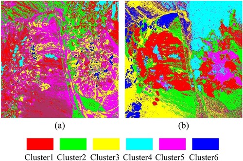(6) $SAM=acos\left({\displaystyle \frac{{\sum }_{k=1}^N{x}_{ik}{x}_{jk}}{x_{i}F\cdot x_{j}F}}\right)$(6) where $x_{ik}$ and $x_{jk}$ are the elements of $x_i$ and $x_j$, respectively. Moreover, the clustering result of improved k-means based on BD rather than the original HSI was used as the reference map. It can be seen from Figure 3 that compared with the mineral distribution map, the clustering result of conventional k-means is disordered, while the clustering result of improved k-means can efficiently reflect the spatial distribution of various mineral types. Specifically, compared with conventional k-means, the improved k-means can more accurately find alunite, kaolinite, muscovite, calcite, chalcedony, background pixels, and the mixed pixels of calcite and montmorillonite. This is because BD highlights the differences among various mineral types, and unlike Euclidean distance, SAM is not sensitive to dimensionality.

Figure 3. Clustering results of conventional k-means (a) and improved k-means (b).

3.3.2. Calculation of the coincidence degree

In this study, two external clustering indexes, including ARI and AMI, were used to find the eigenvectors that match the data distribution of the reference map. The ARI and AMI are the adjustment of the Rand index and mutual information (MI), respectively. They have a constant baseline equal to 0 when the partitions are random and independent, and they are equal to 1 when the compared partitions are identical. To calculate the ARI and AMI, the information on cluster overlaps between two partitions (i.e. U and G) can be summarized in the form of a $R\times C$ contingency table (Vinh, Epps, and Bailey 2009), where $n_{ij}$ denotes the number of objects that are common to clusters $U_i$ and $G_j$.

Based on Table 1, ARI and AMI can be calculated as follows. (7) $ARI={\displaystyle \frac{{\sum }_{ij}\left(\begin{array}{c}{n}_{ij}\\ 2\end{array}\right)-\left[{\sum }_i\left(\begin{array}{c}{a}_i\\ 2\end{array}\right){\sum }_j\left(\begin{array}{c}{b}_j\\ 2\end{array}\right)\right]/\left(\begin{array}{c}N\\ 2\end{array}\right)}{{\displaystyle \frac{1}{2}\left[{\sum }_i\left(\begin{array}{c}{a}_i\\ 2\end{array}\right)+{\sum }_j\left(\begin{array}{c}{b}_j\\ 2\end{array}\right)\right]-\left[{\sum }_i\left(\begin{array}{c}{a}_i\\ 2\end{array}\right){\sum }_j\left(\begin{array}{c}{b}_j\\ 2\end{array}\right)\right]/\left(\begin{array}{c}N\\ 2\end{array}\right)}}}$(7) (8) $MI=\sum _{i=1}^R\sum _{j=1}^C{p}_{ij}\log \left({\displaystyle \frac{p_{ij}}{p_i\times p_j}}\right)$(8) (9) $H(U)=-\sum _{i=1}^R{p}_i\log (p_i)$(9) (10) $H(G)=-\sum _{j=1}^C{p}_j\log (p_j)$(10) (11) $AMI={\displaystyle \frac{MI-E[MI]}{max(H(U),H(G))-E[MI]}}$(11) where $H(U)$ and $H(G)$ are the entropies associated with the clustering $U$ and $G$, respectively; $p_i={\displaystyle \frac{|U_i|}{N}}$ is the probability that a point falls into cluster $U_i$; $p_j={\displaystyle \frac{|G_j|}{N}}$ is the probability that a point falls into cluster $G_j$; and $p_{ij}={\displaystyle \frac{|U_i\cap G_j|}{N}}$ denotes the probability that a point belongs to cluster $U_i$ in $U$ and cluster $G_j$ in $G$. The value range of the ARI and AMI is [−1, 1]. The larger the values of ARI and AMI are, the more consistent the spatial distribution of an eigenvector is with that of the reference map. That is, the eigenvectors with large ARI or AMI values should be used for spectral clustering.

Table 1. Contingency table.

U/G	$G_1$	$G_2$	$\cdots$	$G_C$	Sums
$U_1$	$n_{11}$	$n_{12}$	$\cdots$	$n_{1C}$	$a_1$
$U_2$	$n_{21}$	$n_{22}$	$\cdots$	$n_{2C}$	$a_2$
$⋮$	$⋮$	$⋮$	$\ddots$	$⋮$	$⋮$
$U_R$	$n_{R1}$	$n_{R2}$	$\cdots$	$n_{RC}$	$a_R$
Sums	$b_1$	$b_2$	$\cdots$	$b_c$	$\sum _{ij}{n}_{ij}=N$

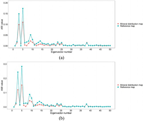
It can be seen from Figure 4 that for ARI or AMI, the overall curve shapes based on the mineral distribution map and reference map are highly similar. Specifically, the ARI and AMI values of the third and fifth original eigenvectors are significantly higher than those of other eigenvectors. This means that compared with other eigenvectors, the third and fifth original eigenvectors can better reflect the spatial distribution of various mineral types and should be placed at the top of the final eigenvector list. Furthermore, with the exception of these two eigenvectors, the ARI and AMI values of the ninth original eigenvectors are also considerably higher than those of other eigenvectors. Therefore, the ninth original eigenvector should be ranked third in the final eigenvector list.

Figure 4. ARI (a) and AMI (b) values of unsorted original eigenvectors based on the mineral distribution map and reference map.

3.3.3. Eigenvector selection based on the coincidence degree of data distribution

Figure 5 shows a flowchart of CDES. It can be seen that CDES mainly includes four steps: (1) performing improved k-means clustering for BD and all eigenvectors; (2) calculating the ARI and AMI values between the reference map and the clustering result of each eigenvector; (3) ranking eigenvectors in descending order according to their ARI or AMI values, and thus the final eigenvector list can be obtained; and (4) selecting the first $M$ eigenvectors with high coincidence degree for clustering according to the differences of ARI or AMI values.

Figure 5. Flowchart of CDES

Figure 6 shows the scatter diagram for determining the $M$ value. It can be seen from Figure 6(c) and (d) that the difference values of ARI and AMI are close to 0 from the 5th and 6th bands, respectively. This means that in the final eigenvector list, the eigenvectors starting from the fifth or sixth have no obvious difference in reflecting the spatial distribution of various types. Therefore, there is no need to continue to select eigenvectors. That is, $M$ should be set to 5 or 6. In addition, it can be seen from Figure 6(a) and (b) that the fifth point of ARI curve and the sixth point of AMI curve are both at the most curved part, indicating that the $M$ value can be automatically determined by calculating the maximum curvature of the ARI or AMI curves.

Figure 6. Scatter diagram for determining the $M$ value. The red dot represents the point with the maximum curvature.

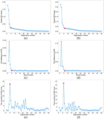
For discrete data, two methods are usually used to obtain the point with the maximum curvature. The first method calculates the first and second derivatives of discrete data by gradient, and then the curvature of each discrete point is calculated according to the curvature formula (Arnau, Ibanez, and Monterde 2017). The second method uses the radius of the circumcircle of three adjacent points to calculate the curvature of each discrete point, which makes this method sensitive to small burrs. The first method uses the central difference quotient to compute the gradient, and the central difference quotient is obtained by averaging, which renders the curvature calculated by gradient method insensitive to small burrs. Therefore, in this study, the gradient method was used to calculate the curvature of the ARI and AMI curves. Furthermore, as the dimensions of x-axis and y-axis in Figure 6(a) and (b) are quite different, normalization is required before calculating curvature. Figure 6(e) and (f) show that the curvature of the fifth point in ARI curve is the largest, while the curvature of the sixth point in AMI curve is considerably larger than those of other points.

Although the reference map can well reveal the differences of various mineral types, the eigenvector selection results of CDES are not fixed, because the clustering results of k-means depend heavily on the initial cluster centers. That is, different initial cluster centers may lead to different eigenvector selection results. Although several classical k-means initialization methods, such as Macqueen approach (MacQueen 1967), Kaufman approach (Kaufman and Rousseeuw 1990), CCIA (Shehroz and Amir 2004), k-means++ (Arthur and Vassilvitskii 2007), and MinMax approach (Tzortzis and Likas 2014) have been developed, these methods either have high computational complexity and cannot be used for large-scale datasets, or have randomness and cannot obtain a definite initialization solution.

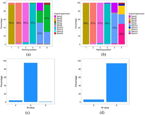
Despite the randomness of k-means clustering, Figure 7(a) and (b) show that there is always a dominant eigenvector at a certain ranking position. In particular, for ARI and AMI, the probabilities that the fifth, third, ninth, and tenth original eigenvectors are selected for spectral clustering are all greater than 90%. Therefore, to address the instability of CDES in selecting eigenvectors, we proposed a CDES method based on multiple random clustering (CDMR). Five steps are included in this method: (1) performing multiple random k-means clustering on all eigenvectors and BD, and the number of k-means clustering, called $\alpha$ for short, is set to 100; (2) calculating the ARI and AMI values between the reference map and the clustering result of each eigenvector; (3) ranking eigenvectors in descending order according to the ARI or AMI values; (4) calculating the frequency of each eigenvector at each ranking position and constructing the final eigenvector list using the eigenvectors with the largest frequency at each ranking position; (5) selecting the first $M$ eigenvectors with high coincidence degree for clustering, where the $M$ value with the largest frequency was used as the final eigenvector number. Figure 7(c) and (d) show that in 100 random clustering, the $M$ values determined by ARI include 4, 5, and 6, most of which are 5, while the $M$ values determined by AMI include 5 and 6, most of which are 6. That is, the final $M$ values determined by ARI and AMI are 5 and 6, respectively.

Figure 7. Bar diagram for selecting the eigenvectors stably. Here, (a) and (b) are the eigenvector selection results of ARI and AMI based on 100 random k-means clustering, respectively, and the percentage in the bar graph represents the maximum probability that an eigenvector is selected at each ranking position. (c) and (d) are the $M$ values determined by calculating the maximum curvature of the ARI and AMI curves, respectively.

To comprehensively analyse the stability of CDMR in eigenvector selection, the initial cluster centers of improved k-means should cover all pixels in the AVIRIS image as far as possible. Therefore, CDMR was performed 175 (i.e. $(350\times 350)/(\alpha \times 7))$) times, and a total of 122,500 (i.e.$175\times (\alpha \times 7)$) non-repeating pixels were used as the initial cluster centers, covering the entire AVIRIS image. Moreover, the CDES methods based on random and classical k-means++ initialization, which are called CDRA and CDKP respectively, were used in spectral clustering for comparison with CDMR. Thus, CDRA, CDKP, CDMR, and two external clustering indexes constitute six CDES eigenvector selection methods, including CDRA-ARI, CDRA-AMI, CDKP-ARI, CDKP-AMI, CDMR-ARI, and CDMR-AMI. The pseudocodes for CDRA, CDKP, and CDMR are shown in Algorithm 2, Algorithm 3, and Algorithm 4, respectively. It should be noted that the difference between k-means in Algorithm 2 and k-means++ in Algorithm 3 is only in the initialization method (i.e. step 1 in Algorithm 1), and other steps are completely consistent.

Algorithm 2: CDRA

Input: All eigenvectors $V=\{v^i{\}}_{i=1}^B$, BD, number of clusters $K$

Output: First $M$ eigenvectors with high coincidence degree

1: ${\delta }^b$ = k-means(BD, $K$) // perform improved k-means clustering on BD

2: for each eigenvector $v^i$ do

3:  ${\delta }^i$ = k-means($v^i,K$) // perform improved k-means clustering on each eigenvector

4:  //calculate ARI or AMI values between each eigenvector and BD

5: Calculate $ARI({\delta }^i,{\delta }^b)$ or $AMI({\delta }^i,{\delta }^b)$ values using (7) and (11)

6: end for

7: EL = sort(ARI or AMI, ‘descend’) // get the eigenvector list by descending ARI or AMI values

8: $M$ = argmax(curvature(ARI or AMI)) // get the number of selected eigenvectors

9: return EL(1:$M$)

Algorithm 3: CDKP

Input: All eigenvectors $V=\{v^i{\}}_{i=1}^B$, BD, number of clusters $K$

Output: First $M$ eigenvectors with high coincidence degree

1: ${\delta }^b$ = k-means++(BD, $K$) // perform improved k-means clustering on BD

2: for each eigenvector $v^i$ do

3:  ${\delta }^i$ = k-means++($v^i,K$) // perform improved k-means clustering on each eigenvector

4:  // calculate ARI or AMI values between each eigenvector and BD

5:  Calculate $ARI({\delta }^i,{\delta }^b)$ or $AMI({\delta }^i,{\delta }^b)$ values using (7) and (11)

6: end for

7: EL = sort(ARI or AMI, ‘descend’) // get the eigenvector list by descending ARI or AMI values

8: $M$ = argmax(curvature(ARI or AMI)) // get the number of selected eigenvectors

9: return EL(1:$M$)

Algorithm 4: CDMR

Input: All eigenvectors $V=\{v^i{\}}_{i=1}^B$, BD, number of clusters $K$

Output: First $M$ eigenvectors with high coincidence degree

1: ${\delta }^b$ = k-means(BD, $K$) // perform improved k-means clustering on BD

2: for j = 1 to $\alpha$ do

3:  for each eigenvector $v^i$ do

4:   ${\delta }^i$ = k-means($v^i,K$) // perform improved k-means clustering on each eigenvector

5:   // calculate ARI or AMI values between each eigenvector and BD

6:   Calculate $ARI({\delta }^i,{\delta }^b)$ or $AMI({\delta }^i,{\delta }^b)$ values using (7) and (11)

7:  end for

8:  EA(j) = sort(ARI or AMI, ‘descend’) // get the eigenvector list by descending ARI or AMI values

9:  MA(j) = argmax(curvature(ARI or AMI)) // get the number of selected eigenvectors

10: end for

11: EL = mode(EA) // the eigenvectors with the largest frequency

12: $M$ = mode(MA) // the $M$ value with the largest frequency

13: return EL(1:$M$)

3.3.4. Computational complexity

The calculation process of CDES mainly includes k-means clustering and coincidence calculation. The computational complexity of k-means is $O(NKBt)$, where t is the number of iterations until convergence is achieved. The computational complexity of ARI and AMI is $O(N)$. Thus, the computational complexity of CDMR is $O(NKBt+\alpha B(NKt+N))$, which is linearly related to N.

3.4. Matching

In this paper, SCGA was used to match the cluster centers of the second k-means with USGS mineral spectral library to obtain the final mineral mapping results. SCGA could achieve promising mapping results at both high and low signal-to-noise ratios. (12) $SCA=acos\left(\left({\displaystyle \frac{{\sum }_{i=1}^N(x_{ti}-\overline{x_t})\ast (x_{ri}-\overline{x_r})}{x_t-\overline{x_t}\cdot x_r-\overline{x_r}}+1}\right)/2\right)$(12) (13) $S{G}_t=(x_{t2}-x_{t1},x_{t3}-x_{t2},\dots ,x_{tn}-x_{t(n-1)})$(13) (14) $S{G}_r=(x_{r2}-x_{r1},x_{r3}-x_{r2},\dots ,x_{rn}-x_{r(n-1)})$(14) (15) $SGA=acos\left(\frac{{\displaystyle {\sum }_{i=1}^{(N-1)}S{G}_{ti}\ast S{G}_{ri}}}{S{G}_{t_F\cdot S{G}_{r_F}}}\right)$(15) (16) $SCGA=sqrt(SC{A}^2+SG{A}^2)$(16) where $x_t$ and $x_r$ represent the target and reference spectral vectors, respectively; ${\overline{x}}_t$ and ${\overline{x}}_r$ are the mean values of $x_t$ and $x_r$, respectively; and $S{G}_t$ and $S{G}_r$ are the spectral gradient vectors of $x_t$ and $x_r$, respectively.

3.5. Accuracy assessment

Overall accuracy (OA) and Kappa coefficient (KC) (Congalton 1991), calculated from the confusion matrix, are typically used to evaluate the HSI classification accuracy. OA considers the number of correctly classified pixels in the diagonal direction of the confusion matrix, while KC considers all kinds of missing and wrong pixels outside the diagonal direction. (17) $OA=\sum _{i=1}^r{s}_{ii}/T$(17) (18) $KC={\displaystyle \frac{T{\sum }_{i=1}^r{s}_{ii}-{\sum }_{i=1}^r(s_{i+}{s}_{+i})}{T^2-{\sum }_{i=1}^r(s_{i+}{s}_{+i})}}$(18) where r is the number of mineral types; $s_{ii}$ is the sum of the confusion matrix diagonal; $T$ is the total number of samples; $s_{i+}$ is the sum of the ith predicted mineral, and $s_{+i}$ is the sum of the ith mineral in the sample.

4. Results

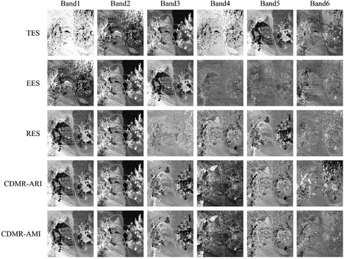
Figure 8 shows the eigenvector selection results of various methods. It can be seen that among the first six eigenvectors selected by TES, the first, second, fourth, and sixth original eigenvectors cannot reveal the differences of various types, while the third and fifth original eigenvectors can better reflect the spatial distribution of various mineral types than other eigenvectors. Therefore, the third and fifth eigenvectors should be placed first, which is consistent with the analysis results in Figure 4. Although EES puts these two eigenvectors forward compared with TES, it still does not rank them in the first place, and other eigenvectors selected by EES cannot efficiently reflect the mineral distribution. For CDMR-ARI, the first six eigenvectors correspond to the fifth, third, ninth, tenth, fourteenth, and eighth original eigenvectors respectively, while the first six eigenvectors of CDMR-AMI correspond to the fifth, third, ninth, tenth, fourteenth, and fifteenth original eigenvectors respectively. That is, the first five eigenvectors selected by CDMR-ARI and CDMR-AMI are completely consistent. Furthermore, CDMR not only puts the third and fifth original eigenvectors in the first place, but also finds other eigenvectors that can reflect the spatial distribution of various mineral types to some extent. In particular, among the four eigenvector selection methods, only CDMR could find the tenth original eigenvector (i.e. band4 of CDMR-ARI or CDMR-AMI) that can well reflect the spatial distribution of calcite. Although RES also puts the third and fifth original eigenvectors in the first place, it puts the ninth original eigenvector in the fifth position, and other two eigenvectors (i.e. the fiftieth and forty-seventh original eigenvectors) cannot effectively reflect the mineral distribution.

Figure 8. First six eigenvectors selected by various eigenvector selection methods.

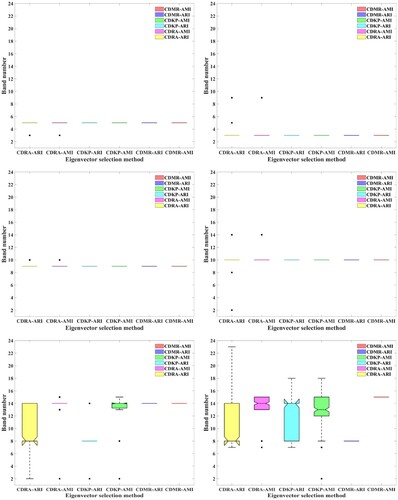
In terms of the stability of the six CDES methods in eigenvector selection, it can be seen from Figure 9 that although CDKP can obtain stable eigenvector selection results in the first four ranking positions, it still has some outliers in the fifth or sixth ranking position. Furthermore, regardless of which coincidence degree indices are used for eigenvector selection, CDRA always has some outliers because of the randomness of k-means, while CDMR has no outliers and can obtain stable eigenvector selection results. This means that through multiple random clustering, CDES can eliminate the influence of the randomness of k-means on the stability of eigenvector selection.

Figure 9. Boxplots for analysing the stability of the six CDES methods in eigenvector selection. (a), (b), (c), (d), (e), and (f) are the first to the sixth selected eigenvectors, respectively.

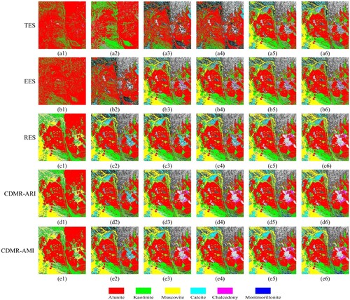
Figure 10 shows the mineral mapping results of spectral clustering. In particular, the initial cluster centers of the second k-means were fixed so that these mapping results could be compared. It can be seen that qualitatively, regardless of which eigenvectors are used for clustering, CDMR-ARI and CDMR-AMI always perform better than TES and EES in mineral mapping. Specifically, RES, CDMR-ARI, and CDMR-AMI have same mapping results based on the first two eigenvectors, which obviously contain more mineral types than those of TES and EES. When the first three and four eigenvectors are used for spectral clustering, TES performs worst among the four eigenvector selection methods, and RES, CDMR-ARI, and CDMR-AMI find more muscovite and calcite pixels than TES and EES. Moreover, CDMR-ARI and CDMR-AMI identify more chalcedony pixels than TES, EES, and RES based on the first three or four eigenvectors. When the first five or six eigenvectors are used for clustering, the mineral mapping result of TES is greatly improved, and TES and EES have similar mapping performance. Nevertheless, CDMR still performs much better than TES and EES in mapping results, and could find more muscovite, calcite, and chalcedony pixels.

Figure 10. Mineral mapping results of spectral clustering. (a1–a6), (b1–b6), (c1–c6), (d1–d6), and (e1–e6) are the mineral mapping results of TES, EES, RES, CDMR-ARI, and CDMR-AMI respectively. The mapping results of columns 1 to 6 are based on the first to the first six eigenvectors respectively.

Table 2 shows the mineral mapping accuracies of various eigenvector selection methods. In particular, the mapping accuracies of the six CDES methods were averaged from 175 mineral mapping results. Quantitatively, regardless of which eigenvectors or coincidence degree indices are used for spectral clustering, CDRA, CDKP, and CDMR always perform better than TES and EES in mapping accuracies, and CDRA performs slightly worse than CDKP and CDMR in average mapping accuracies. Although RES has the same mapping accuracies with CDKP and CDMR based on the first two eigenvectors, the average mapping accuracies of CDES are higher than those of RES when the eigenvector number is greater than 2. Furthermore, when the eigenvector number is in the range of 1 to 4, CDKP and CDMR have the same mapping accuracy. In particular, when the first two eigenvectors are used for clustering, the KC values of CDKP and CDMR can be approximately 47.8% and 42.9% higher than those of TES and EES, respectively. When the first four eigenvectors are used for clustering, the OA values of CDKP and CDMR are approximately 44.0%, 12.8%, and 8.4% higher than those of TES, EES, and RES respectively, and the KC values of CDKP and CDMR are approximately 56.3%, 15.5%, and 10.5% higher than those of TES, EES, and RES respectively. Although the mapping result of TES is improved considerably after adding the fifth original eigenvector, the OA and KC values of CDMR can also be approximately12% and 14% higher than those of TES. In addition, among all eigenvector selection methods, CDMR based on the first five eigenvectors has the highest mapping accuracy.

Table 2. Mineral mapping accuracies of various eigenvector selection methods.

	OA						KC
	1	2	3	4	5	6	1	2	3	4	5	6
TES	0.42	0.40	0.41	0.41	0.73	0.73	0.14	0.20	0.24	0.25	0.66	0.66
EES	0.38	0.41	0.72	0.72	0.72	0.72	0.09	0.25	0.65	0.65	0.66	0.65
RES	0.62	0.75	0.77	0.77	0.78	0.79	0.52	0.68	0.70	0.70	0.72	0.74
CDRA-ARI	0.61	0.74	0.81	0.85	0.81	0.82	0.51	0.68	0.76	0.80	0.76	0.77
CDRA-AMI	0.61	0.74	0.81	0.84	0.83	0.81	0.52	0.68	0.76	0.80	0.79	0.76
CDKP-ARI	0.62	0.75	0.82	0.85	0.80	0.83	0.52	0.68	0.77	0.81	0.75	0.78
CDKP-AMI	0.62	0.75	0.82	0.85	0.84	0.80	0.52	0.68	0.77	0.81	0.79	0.75
CDMR-ARI	0.62	0.75	0.82	0.85	0.86	0.84	0.52	0.68	0.77	0.81	0.82	0.80
CDMR-AMI	0.62	0.75	0.82	0.85	0.86	0.85	0.52	0.68	0.77	0.81	0.82	0.81

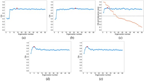
Figure 11 shows the mapping accuracies of various eigenvector selection methods with different eigenvectors. It can be seen that compared with CDMR, the OA curves of TES, EES, and RES do not have obvious peak points, indicating that for these eigenvector selection methods, it is not easy to determine the optimal $M$ values corresponding to their maximum mapping accuracies. Actually, the optimal $M$ values of EES and RES are 27 and 6, respectively, instead of 10 and 17. The optimal $M$ values of TES is 14. Furthermore, 14, 17, or 27 eigenvectors are too large to meet the requirements of dimensionality reduction for HSIs, and their maximum mapping accuracies are also lower than those of CDMR. For CDMR, the mapping accuracies increase monotonically with the increase of the eigenvector number until the maximum mapping accuracy is achieved when the eigenvector number is 5, and subsequently the mapping accuracy begins to decline. This indicates that for the AVIRIS image, the $M$ value can be accurately determined by calculating the maximum curvature of the ARI curve. Although the $M$ value determined by AMI is 6, it can be seen from Table 2 and Figure 11 that the CDMR mapping accuracies based on the first four, five, and six eigenvectors are actually very close.

Figure 11. Mapping accuracies of TES (a), EES (b), RES (c), CDMR-ARI (d), and CDMR-AMI (e) with different eigenvectors. In particular, the coral line in figure (c) represents the relevance values of each eigenvector, and the threshold of 0.5 corresponds to the first seventeen eigenvectors. The red dot represents the point with the maximum mapping accuracy.

Table 3 presents the running time of various eigenvector selection methods on 6-core i5-8500 processors and 64-bit operating systems. In Table 3, when computing the running time for CDMR, improved k-means was performed 100 times. Specifically, the running time of TES is 0 because it directly selects the eigenvectors with the smallest eigenvalues. In terms of the running time of other eigenvector selection methods, EES and RES respectively take more than 10 and 45 h to complete the eigenvector selection process, while CDRA, CDKP, and CDMR only need approximately 0.2, 38, and 16 min to obtain better eigenvector selection results. Compared with EES and RES, the running time of CDRA is very short and can even be ignored, and more than 97% and 99% of the eigenvector selection time can be saved by CDMR. In addition, the running time of CDMR only accounts for 43% of that of CDKP, which means that compared with CDKP, CDMR can obtain more stable eigenvector selection results in less time.

Table 3. Running time of various eigenvector selection methods.

Selection Method	Time(min)	Selection Method		Time(min)
TES	0.00	CDRA	ARI	0.17
			AMI	0.17
EES	607.19	CDKP	ARI	37.51
			AMI	37.53
RES	2753.39	CDMR	ARI	16.22
			AMI	16.38

5. Discussion

In terms of the mineral mapping accuracy, CDES performs better than TES, EES, and RES, indicating that the eigenvectors selected based on the coincidence degree of data distribution can more effectively reveal the differences between various mineral types. That is, by prioritizing original eigenvectors according to the coincidence degree values, CDES can effectively solve the first critical issue of spectral clustering eigenvector selection, which is to put informative eigenvectors in the first place. Furthermore, Figure 11 reveals that the $M$ values determined by calculating the maximum curvature of the ARI or AMI curves are equal to or very close to the optimal number of eigenvectors. That is, by calculating the maximum curvature of the coincidence degree curves, CDES can also effectively solve the second critical issue of spectral clustering eigenvector selection, which is to automatically determine the eigenvector number used for clustering. In addition, when the values of $M$ obtained from the maximum curvature of ARI and AMI curves are different, the final $M$ value can be determined by calculating the mode of $M$ values obtained by CDMR-ARI and CDMR-AMI in multiple random clustering. In this paper, when $M$ is 4, 5, and 6, the corresponding frequencies are 4, 101, and 95, respectively. Therefore, the final $M$ value is 5, which is the optimal number of eigenvectors.

In terms of the eigenvector selection efficiency, it is clear that the selection efficiency of EES and RES is unacceptable in practical applications, which means that they are not feasible for use in the eigenvector selection of large-scale datasets. Due to the fast-clustering nature of k-means, CDES performs significantly better than EES and RES in eigenvector selection efficiency. Specifically, since RES uses expectation maximization to iteratively estimate the parameters of the Gaussian distribution of each eigenvector, its running time is much longer than those of other eigenvector selection methods. Although EES outperforms RES in eigenvector selection efficiency, its running time is still much longer than that of CDES, because EES needs to calculate the similarity between two points in each eigenvector. Among various CDES methods, CDRA requires much less time to complete the eigenvector selection process than CDKP and CDMR, because it only needs to run the improved k-means randomly once. However, the cost is the instability of CDRA in selecting eigenvectors. Generally, k-means++ uses the roulette algorithm to eliminate the influence of image outliers on clustering results, which renders the running time of CDKP much longer than CDRA and CDMR. In fact, CDMR can also eliminate the influence of image outliers on the eigenvector selection by multiple random clustering, because the image outliers only account for a very small part of the whole HSI. CDMR is actually a combination of multiple CDRAs, and its eigenvector selection time is related to the $\alpha$ value. The larger the $\alpha$ value, the longer the running time. Even so, in practical application, the $\alpha$ value should be set to be larger to ensure the stability of eigenvector selection. In addition, ARI-based and AMI-based CDES methods have no obvious difference in eigenvector selection efficiency.

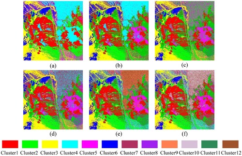
In addition to the initial cluster centers, the clustering results of k-means are also limited by the indeterminacy of $K$. Unfortunately, there is still no definitive answer to determine the optimal $K$ value at present. Fortunately, for CDES, there is no need to determine the $K$ value accurately. It can be seen from Figure 12 that when $K$ is set to 8, 9, 10, 11, and 12, the clustering results of improved k-means can also well reflect the mineral distribution. Although the clustering result of improved k-means with six clusters lost the spatial distribution of chalcedony, it can still well reflect the spatial distribution of other mineral types.

Figure 12. Clustering results of improved k-means with different $K$ values. (a), (b), (c), (d), (e), and (f) are the clustering results when $K$ is 6, 8, 9, 10, 11, and 12, respectively.

Table 4 presents the eigenvector selection results and corresponding mapping accuracies of CDMR with different $K$ values. It can be seen that for CDMR-ARI, five eigenvectors including the fifth, third, ninth, tenth, and fourteenth original eigenvectors are used for clustering when $K$ is in the range of 8 to 12. Although the positions of individual eigenvectors have changed, the mapping accuracy of CDMR-ARI still remains unchanged. Furthermore, although the ranking positions of the eighth and fourteenth eigenvectors are reversed when $K$ is 6, the mapping accuracies are still very close to those when $K$ is 7. For CDMR-AMI, irrespective of the $K$ value, the first five selected eigenvectors are completely consistent, which also include the fifth, third, ninth, tenth, and fourteenth original eigenvectors. Therefore, when $K$ is between 10 and 12, CDMR-AMI has the same mapping accuracy with CDMR-ARI. When $K$ is in the range of 6 to 9, six eigenvectors including the thirteenth and fifteenth original eigenvectors were selected by CDMR-AMI for clustering, and the corresponding mapping accuracies are also close to the maximum mapping accuracy.

Table 4. Eigenvector selection results and corresponding mapping accuracies of CDMR with different $K$ values.

	CDMR-ARI						CDMR-AMI
K	6	8	9	10	11	12	6	8	9	10	11	12
Band1	5	5	5	5	5	5	5	5	5	5	5	5
Band2	3	3	3	3	3	3	3	3	3	3	3	3
Band3	9	9	9	9	9	9	9	9	9	9	9	9
Band4	10	10	10	14	14	14	10	10	10	10	10	10
Band5	8	14	14	10	10	10	14	14	14	14	14	14
Band6	14	\	\	\	\	\	13	15	15	\	\	\
OA	0.84	0.86	0.86	0.86	0.86	0.86	0.83	0.85	0.85	0.86	0.86	0.86
KC	0.80	0.82	0.82	0.82	0.82	0.82	0.78	0.81	0.81	0.82	0.82	0.82

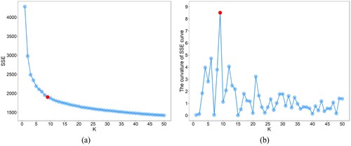
In cluster analysis, the elbow method is the most common method used to determine the optimal $K$ value (Bholowalia and Kumar 2014). This method first plots the SSE values with changing $K$ (i.e. Figure 13(a)), and then the elbow of the SSE curve is used as the cluster number. However, the elbow cannot always be unambiguously identified. Actually, the elbow of the SSE curve corresponds to the most curved part, which can also be located by calculating the maximum curvature. Similarly, since the dimension difference between SSE and $K$ values is quite different, normalization is required before calculating the curvature. Figure 13(b) shows that when $K$ is 9, the curvature of the SSE curve is the highest. Furthermore, Figure 12 shows that the clustering result of improved k-means with nine clusters can well reflect the spatial distribution of various mineral types, and in Table 4, the mapping accuracies of CDMR when $K$ is 9 are equal to or very close to the maximum mapping accuracy. Therefore, for CDES, the $K$ value of the improved k-means can be determined by calculating the maximum curvature of the SSE curve. In addition, for HSIs, the $K$ value can also be automatically determined by clustering-matching or spectral matching method, which needs the support of spectral library.

Figure 13. SSE (a) and curvature (b) curves of the AVIRIS image. The red dot represents the point with the maximum curvature.

To sum up, compared with classical eigenvector selection methods of spectral clustering, CDES can find the features with detailed discriminative information more effectively and rapidly, thereby improving the HSI classification accuracy and efficiency of spectral clustering. It should be noted that in the implementation of CDES, the acquisition of the reference map is very important. Before using improved k-means to obtain the reference map, it is necessary to enhance the feature differences of various types. As the most commonly used method to enhance the spectral absorption features, CR is generally performed on the reflectance spectral curves of ground objects. Therefore, it is necessary to perform atmospheric correction on HSI to obtain surface reflectance data before using CDES to select eigenvectors.

Considering that k-means easily falls into local optimal solution, the clustering algorithms with global search ability may be used to generate the reference map. However, complex clustering algorithms will reduce the eigenvector selection efficiency of CDES. Moreover, although other clustering algorithms do not necessarily select the initial cluster centers or $K$ values, they still need to set other clustering parameters. That is, CDES based on other clustering algorithms still requires solving the problem of selecting eigenvectors stably. In addition, the mapping accuracies in Table 2 are not very high. This is because the clustering result of spectral clustering is not only affected by the eigenvector selection methods, but also by the Nyström sampling method, which is another important research direction of spectral clustering. Future research on more efficient Nyström sampling methods will help further improve the spectral clustering results.

6. Conclusion

To address critical concerns in the eigenvector selection of spectral clustering, this study proposes an intuitive eigenvector selection method based on the coincidence degree of the data distribution. Firstly, the clustering result of improved k-means, which uses cosine similarity instead of Euclidean distance for clustering, is used as the reference map. Then, the eigenvectors that are highly consistent with the data distribution of the reference map are selected for spectral clustering. The hyperspectral mineral mapping results of Cuprite show that compared with the commonly used eigenvectors, the eigenvectors selected based on the coincidence degree of data distribution can more effectively reveal the differences of various types, thus improving the hyperspectral image classification accuracy of spectral clustering. Moreover, CDES also performs much better than the eigenvector selection methods based on entropy and relevance in selection efficiency, and can save more than 99% of the eigenvector selection time at most. Although the clustering results of k-means depend heavily on the initial cluster centers, CDES can obtain stable eigenvector selection results by multiple random clustering. In addition, since k-means is an unsupervised classification method, CDES is independent of the ground truth map and provides a novel solution for autonomous feature selection of hyperspectral images. Future research on more efficient Nyström sampling methods may help further improve the selected eigenvectors.

Acknowledgements

The author would like to thank Sudeep Sahadevan for providing the source code of the relevance eigenvector selection method.

Disclosure statement

No potential conflict of interest was reported by the author(s).

Data availability statement

The data that support the findings of this study are openly available in https://www.ehu.eus/ccwintco/index.php?title=Hyperspectral_Remote_Sensing_Scenes.

Additional information

Funding

This work was supported by the [National Key Research and Development Program] under Grant [number 2019YFE0126700]; [Shandong Provincial Natural Science Foundation] under Grant [number ZR2020QD018].

References

- Arnau, X. G., M. V. Ibanez, and J. Monterde. 2017. “Curvature Approximation from Parabolic Sectors.” Image Analysis & Stereology 36 (3): 233–241. https://doi.org/10.5566/ias.1702.
- Arthur, D., and S. Vassilvitskii. 2007. “k-means++: The Advantages of Careful Seeding.” Proceedings of the Eighteenth Annual ACM-SIAM Symposium on Discrete Algorithms 1027–1035. https://doi.org/10.1145/1283383.1283494.
- Bachmann, C. M., T. L. Ainsworth, and R. A. Fusina. 2005. “Exploiting Manifold Geometry in Hyperspectral Imagery.” IEEE Transactions on Geoscience and Remote Sensing 43 (3): 441–454. https://doi.org/10.1109/TGRS.2004.842292.
- Bholowalia, P., and A. Kumar. 2014. “EBK-means: A Clustering Technique Based on Elbow Method and K-Means in WSN.” International Journal of Computer Applications 105 (9): 17–24. https://doi.org/10.5120/18405-9674.
- Cao, Y., T. Yomo, and B. W. Ying. 2020. “Clustering of Bacterial Growth Dynamics in Response to Growth Media by Dynamic Time Warping.” Microorganisms 8 (3): 331. https://doi.org/10.3390/microorganisms8030331.
- Chen, X. F., T. A. Warner, and D. J. Campagna. 2007. “Integrating Visible, Near-Infrared and Short-Wave Infrared Hyperspectral and Multispectral Thermal Imagery for Geological Mapping at Cuprite, Nevada.” Remote Sensing of Environment 110 (3): 344–356. https://doi.org/10.1016/j.rse.2007.03.015.
- Clark, R. N., G. A. Swayze, T. V. V. King, A. J. Gallagher, and W. M. Calvin. 1993. “The U. S. Geological Survey, Digital Spectral Library: Version 1: 0.2 to 3.0 microns.” U.S. Geological Survey Open File Report 93-592. https://doi.org/10.3133/OFR93592.
- Clark, R. N., G. A. Swayze, K. E. Livo, R. F. Kokaly, S. J. Sutly, J. B. Dalton, R. R. McDougal, and C. A. Gent. 2003. “Imaging Spectroscopy: Earth and Planetary Remote Sensing with the USGS Tetracorder and Expert Systems.” Journal of Geophysical Research: Planets 108 (12): 1–44. https://doi.org/10.1029/2002JE001847.
- Congalton, R. G. 1991. “A Review of Assessing the Accuracy of Classifications of Remotely Sensed Data.” Remote Sensing of Environment 37 (1): 35–46. https://doi.org/10.1016/0034-4257(91)90048-B.
- Filippone, M., F. Camastra, F. Masulli, and S. Rovetta. 2008. “A Survey of Kernel and Spectral Methods for Clustering.” Pattern Recognition 41 (1): 176–190. https://doi.org/10.1016/j.patcog.2007.05.018.
- Fowlkes, C., S. Belongie, F. Chung, and J. Malik. 2004. “Spectral Grouping Using the Nystrom Method.” IEEE Transactions on Pattern Analysis and Machine Intelligence 26 (2): 214–225. https://doi.org/10.1109/TPAMI.2004.1262185.
- Hassanzadeh, A., A. Kaarna, and T. Kauranne. 2018. “Sequential Spectral Clustering of Hyperspectral Remote Sensing Image Over Bipartite Graph.” Applied Soft Computing 73: 727–734. https://doi.org/10.1016/j.asoc.2018.09.015.
- Jia, Hongjie, Shifei Ding, and Mingjing Du. 2017. “A Nyström spectral clustering algorithm based on probability incremental sampling.” Soft Computing 21 (19): 5815–5827. https://doi.org/10.1007/s00500-016-2160-8.
- Kaufman, L., and P. J. Rousseeuw. 1990. “Finding Groups in Data: An Introduction to Cluster Analysis.” Biometrics 47 (2): 1–3. https://doi.org/10.1080/02664763.2023.2220087.
- Kruse, F. A., J. W. Boardman, and J. F. Huntington. 2003. “Comparison of Airborne Hyperspectral Data and EO-1 Hyperion for Mineral Mapping.” IEEE Transactions on Geoscience and Remote Sensing 41 (6): 1388–1400. https://doi.org/10.1109/TGRS.2003.812908.
- Kumar, P., D. K. Gupta, V. N. Mishra, and R. Prasad. 2015. “Comparison of Support Vector Machine, Artificial Neural Network, and Spectral Angle Mapper Algorithms for Crop Classification Using LISS IV Data.” International Journal of Remote Sensing 36 (6): 1604–1617. https://doi.org/10.1080/2150704X.2015.1019015.
- Li, Z., H. Huang, Z. Zhang, and Y. Pan. 2022. “Manifold Learning-Based Semisupervised Neural Network for Hyperspectral Image Classification.” IEEE Transactions on Geoscience and Remote Sensing 60: 1–12. https://doi.org/10.1109/TGRS.2021.3083776.
- Likas, A., N. Vlassis, and J. J. Verbeek. 2003. “The Global k-Means Clustering Algorithm.” Pattern Recognition 36 (2): 451–461. https://doi.org/10.1016/S0031-3203(02)00060-2.
- Liu, Y., L. C. Jiao, and F. Shang. 2013. “An Efficient Matrix Factorization Based Low-Rank Representation for Subspace Clustering.” Pattern Recognition 46 (1): 284–292. https://doi.org/10.1016/j.patcog.2012.06.011.
- MacQueen, J. B. 1967. “Some Methods for Classification and Analysis of Multivariate Observations.” Proceedings of the Symposium on Mathematics and Probability 1: 281–297.
- Ni, L., H. Xu, and X. Zhou. 2020. “Mineral Identification and Mapping by Synthesis of Hyperspectral VNIR/SWIR and Multispectral TIR Remotely Sensed Data with Different Classifiers.” IEEE Journal of Selected Topics in Applied Earth Observations and Remote Sensing 13: 3155–3163. https://doi.org/10.1109/JSTARS.2020.2999057.
- Noomen, M. F., A. K. Skidmore, F. V. D. Meer, and H. H. T. Prins. 2006. “Continuum Removed Band Depth Analysis for Detecting the Effects of Natural gas, Methane and Ethane on Maize Reflectance.” Remote Sensing of Environment 105 (3): 262–270. https://doi.org/10.1016/j.rse.2006.07.009.
- Prakash, A., S. Balasubramanian, and R. R. Sarma. 2013. “Improvised Eigenvector Selection for Spectral Clustering in Image Segmentation.” Proceeding of the Fourth National Conference on Computer Vision, Pattern Recognition, Image Processing and Graphics (NCVPRIPG), 1–4. https://doi.org/10.1109/NCVPRIPG.2013.6776233.
- Ren, Z., L. Sun, and Q. Zhai. 2020. “Improved k-Means and Spectral Matching for Hyperspectral Mineral Mapping.” International Journal of Applied Earth Observation and Geoinformation 91: 102154. https://doi.org/10.1016/j.jag.2020.102154.
- Ren, Z., Q. Zhai, and L. Sun. 2022. “A Novel Method for Hyperspectral Mineral Mapping Based on Clustering-Matching and Nonnegative Matrix Factorization.” Remote Sensing 14 (4): 1042. https://doi.org/10.3390/rs14041042.
- Resmini, R. G., M. E. Kappus, W. S. Aldrich, J. C. Harsanyi, and M. Anderson. 2010. “Mineral Mapping with Hyperspectral Digital Imagery Collection Experiment (HYDICE) Sensor Data at Cuprite, Nevada, U.S.A.” International Journal of Remote Sensing 18 (7): 1553–1570. https://doi.org/10.1080/014311697218278.
- Shehroz, S. K., and A. Amir. 2004. “Cluster Center Initialization Algorithm for K-Means Clustering.” Pattern Recognition Letters 25 (11): 1293–1302. https://doi.org/10.1016/j.patrec.2004.04.007.
- Toussi, S. A., and H. S. Yazdi. 2011. “Feature Selection in Spectral Clustering.” International Journal of Signal Processing, Image Processing and Pattern Recognition 4: 179–194. https://doi.org/10.3758/BF03210519.
- Tzortzis, G., and A. Likas. 2014. “The MinMax k-Means Clustering Algorithm.” Pattern Recognition 47 (7): 2505–2516. https://doi.org/10.1016/j.patcog.2014.01.015.
- Vinh, N. X., J. Epps, and J. Bailey. 2009. “Information Theoretic Measures for Clusterings Comparison: Is a Correction for Chance Necessary?” Proceedings of the 26th Annual International Conference on Machine Learning 1073–1080. https://doi.org/10.1145/1553374.1553511.
- Wang, R., F. Nie, and W. Yu. 2017. “Fast Spectral Clustering with Anchor Graph for Large Hyperspectral Images.” IEEE Geoscience and Remote Sensing Letters 14 (11): 2003–2007. https://doi.org/10.1109/LGRS.2017.2746625.
- Xiang, T., and S. Gong. 2008. “Spectral Clustering with Eigenvector Selection.” Pattern Recognition 41 (3): 1012–1029. https://doi.org/10.1016/j.patcog.2007.07.023.
- Zhang, H., H. Zhai, L. Zhang, and P. Li. 2016. “Spectral-Spatial Sparse Subspace Clustering for Hyperspectral Remote Sensing Images.” IEEE Transactions on Geoscience and Remote Sensing 54 (6): 3672–3684. https://doi.org/10.1109/TGRS.2016.2524557.
- Zhao, F., L. Jiao, H. Liu, X. Gao, and M. Gong. 2010. “Spectral Clustering with Eigenvector Selection Based on Entropy Ranking.” Neurocomputing 73 (10-12): 1704–1717. https://doi.org/10.1016/j.neucom.2009.12.029.
- Zhou, S., X. Liu, C. Zhu, Q. Liu, and J. Yin. 2014. “Spectral Clustering-Based Local and Global Structure Preservation for Feature Selection.” International Joint Conference on Neural Networks, 550–557. https://doi.org/10.1109/IJCNN.2014.6889641.