Local climate zone mapping using remote sensing: a synergetic use of daytime multi-view Ziyuan-3 stereo imageries and Luojia-1 nighttime light data

ABSTRACT

The local climate zone (LCZ) scheme has been widely utilized in regional climate modeling, urban planning, and thermal comfort investigations. However, existing LCZ classification methods face challenges in characterizing complex urban structures and human activities involving local climatic environments. In this study, we proposed a novel LCZ mapping method that fully uses space-borne multi-view and diurnal observations, i.e. daytime Ziyuan-3 stereo imageries (2.1 m) and Luojia-1 nighttime light (NTL) data (130 m). Firstly, we performed land cover classification using multiple machine learning methods (i.e. random forest (RF) and XGBoost algorithms) and various features (i.e. spectral, textural, multi-view features, 3D urban structure parameters (USPs), and NTL). In addition, we developed a set of new cumulative elevation indexes to improve building roughness assessments. The indexes can estimate building roughness directly from fused point clouds generated by both along- and across-track modes. Finally, based on the land cover and building roughness results, we extracted 2D and 3D USPs for different land covers and used multi-classifiers to perform LCZ mapping. The results for Beijing, China, show that our method yielded satisfactory accuracy for LCZ mapping, with an overall accuracy (OA) of 90.46%. The overall accuracy of land cover classification using 3D USPs generated from both along- and across-track modes increased by 4.66%, compared to that of using the single along-track mode. Additionally, the OA value of LCZ mapping using 2D and 3D USPs (88.18%) achieved a better result than using only 2D USPs (83.83%). The use of NTL data increased the classification accuracy of LCZs E (bare rock or paved) and F (bare soil or sand) by 6.54% and 3.94%, respectively. The refined LCZ classification achieved through this study will not only contribute to more accurate regional climate modeling but also provide valuable guidance for urban planning initiatives aimed at enhancing thermal comfort and overall livability in urban areas. Ultimately, this study paves the way for more comprehensive and effective strategies in addressing the challenges posed by urban microclimates.

KEYWORDS:

• Local climate zone
• land cover
• three-dimensional urban structure parameters
• nighttime light
• multi-classifiers

Highlights (for review)

• A method using satellite diurnal and multi-view observations was proposed for LCZ mapping

• ZY-3 across-track modes were first used to assess building roughness

• Daytime incorporating nighttime surface characteristics were employed to enhance land cover and LCZ classifications

• We evaluate the consequence of 3D USPs and NTL on land cover and LCZ mapping

Nomenclature
Nomenclature	=	Definition
LCZ	=	Local Climate Zone
2D	=	two-dimensional
3D	=	three-dimensional
NTL	=	nighttime light
RF	=	Random Forest
USPs	=	Urban Structure Parameters
UHI	=	Urban Heat Island
OA	=	Overall Accuracy
CNN	=	Convolutional Neural Network
WUDAPT	=	World Urban Database and Access Portal Tool
SAR	=	Synthetic Aperture Radar
PolSAR	=	Polarized Synthetic Aperture Radar
DSM	=	Digital Surface Model
ResNet	=	Residual convolutional neural Network
VIIRS	=	Visible Infrared Imager Radiometer Suite
MLCs	=	Multi-classifiers
RTK	=	Real-Time Kinematic
OSM	=	Open Street Map
NNI	=	Nearest Neighbor Index
NDVI	=	Normalized Difference Vegetation Index
RVI	=	Ratio Vegetation Index
DVI	=	Difference Vegetation Index
NDWI	=	Normalized Difference Water Index
MBI	=	Morphological Building Index
MSI	=	Morphological Shadow Index
GLCM	=	Gray Level Co-occurrence Matrix
SVF	=	Sky View Factor
NAD	=	Nadir view
FWD	=	Forward view
BWD	=	Backward view
RBV	=	Radiation Brightness Value
GI	=	Gini Index
UA	=	User Accuracy
PA	=	Producer Accuracy
RB	=	Relative Border
DV	=	Distance to Vegetation
DB	=	Distance to Building
H	=	Height
FB	=	Forward + Back
FN	=	Forward + Nadir
BN	=	Backward + Nadir
NN_A	=	nadir1 + nadir2
NN_B	=	nadir2 + nadir3
RPCs	=	Rational Polynomial Coefficients
eATE	=	enhanced Automatic Terrain Extraction
OLS	=	Ordinary Least Squares
RMSE	=	Root Mean Square Error
BC	=	Building Coverage
VC	=	Vegetation Coverage
SC	=	Soil Coverage
ISC	=	Impervious surface Coverage
WC	=	Water Coverage
BNNI	=	Building Nearest Neighbor Index
VNNI	=	Vegetation Nearest Neighbor Index
SNNI	=	Soil Nearest Neighbor Index
INNI	=	Impervious surface Nearest Neighbor Index
WNNI	=	Water Nearest Neighbor Index
MBH	=	Mean Building Height
MBV	=	Mean Building Volume
MSW	=	Mean Street Width
CAR	=	Canyon Aspect Ratio
FAR	=	Floor Area Ratio
FAI	=	Frontal Area Index
MRB	=	Mean Radiation Brightness
Exp	=	Experiment

1. Introduction

Urbanization has led to a significant rise in the global urban population, with approximately 55% of people currently residing in cities. This figure is projected to increase to 68% by 2050, according to the United Nations (2018). However, the rapid urban growth has resulted in alterations to surface features, increased anthropogenic activities, and changes in energy consumption patterns. These factors have contributed to local climate shifts, such as the urban heat island effect (Cao et al. 2022; Kamali Maskooni et al. 2021). The urban heat island (UHI) phenomenon refers to increased temperatures in urban areas relative to rural areas, and it is a significant concern in urban environments (Lee et al. 2017; Stewart 2011; Voogt and Oke 2003). The lack of quantitative metadata describing the terms ‘urban’ and ‘rural’ limits the effectiveness of comparing UHI effects between different underlying surfaces (Mills et al. 2015). To address this issue, the local climate zone (LCZ) system was proposed by Stewart and Oke (2012) to characterize and describe UHI phenomena.

The LCZ framework classifies land cover into 17 categories, including ten built types and seven natural types, based on factors such as building height, impervious coverages, and human activities related to local climates. LCZs are fundamental spatial units in cities and play a crucial role in urban planning and management applications, such as surface temperature surveys, landscape patterns, urban planning, and urban ecological modeling (Alberti, Weeks, and Coe 2004; Kane et al. 2014; Yao et al. 2017). Therefore, it is essential to develop effective methods for automatic, accurate, and rapid LCZ classification (Hay Chung, Xie, and Ren 2021).

There are two categories and 17 subcategories of LCZs. LCZs 1-10 are primarily classified according to the spatial morphological characteristics of built-up areas, while LCZs A-G have few buildings and consist primarily of natural surface coverages (Stewart and Oke 2012). These 17 LCZ subcategories can meet the minimum classification requirements for urban climatic research. However, the classification of LCZs can be adjusted according to regional characteristics, and the parameter range of some categories can be modified based on local spatial morphological characteristics. Some of the considerations and rationales we used to make this adjustment are regional climate and weather patterns, urban morphology, land use patterns, vegetation cover, topography, data analysis, and expert judgment. It is important to note that any modifications to the LCZ classification are carefully considered and validated to ensure that the adjustments accurately capture local characteristics and improve the usefulness of the classification system for specific regions. We considered 15 types of LCZs, as shown in Table S1.

In recent years, various approaches have emerged to obtain robust and high-quality LCZ maps. With the rapid development of remote sensing technology, satellite observations have become widely used for LCZ classification (Huang et al. 2023). Many methods were used to extract LCZ information employing detailed spatial and spectral information of underlying surfaces provided by satellite imageries, such as object-based image analysis, supervised classification, and deep learning methods (Bechtel and Daneke 2012; Gál, Bechtel, and Unger 2015). For example, Liu and Shi (2020) examined 15 cities across three economic regions in China using Sentinel-2 multi-spectral data with 10 m spatial resolution for LCZ classification. They introduced a deep convolutional neural network, LCZNet, which incorporates residual learning and compressed excitation blocks. They found that the method achieved an overall accuracy (OA) of 88.61%. Chen, Zheng, and Hu (2020) used Chenzhou city, China, as a case study to determine eight urban morphological parameters such as building height, street aspect ratio, and sky view factor. Using semi-automatic algorithms, they achieved an OA value of 69.54%. Rosentreter, Hagensieker, and Waske (2020) developed a new approach to derive LCZ by utilizing multi-temporal Sentinel-2 composites and a high-resolution supervised Convolutional Neural Network (CNN) in eight German cities. Their method achieved a significant improvement in overall accuracy, increasing by 16.5% compared to pixel-based methods and 4.8% compared to texture-based random forest methods. The Convolutional Neural Network model demonstrated robustness in classifying LCZ in unknown cities, achieving an OA value of 86.5% when sufficient training data was available. Additionally, the World Urban Database and Access Portal Tool (WUDAPT) initiative suggested using free Landsat data and a random forest classifier to label LCZs globally at a spatial resolution of 100 m. For LCZ classification, the WUDAPT method is considered the most commonly used method, and this method has become the standard for LCZ mapping, appearing in about 39% of publications (Bechtel et al. 2015; Fernandes et al. 2023). Despite recent advancements in LCZ classification, several key challenges still exist when it comes to the mapping of LCZ. Indeed, there are some noteworthy considerations regarding previous LCZ classification studies. First, it is important to acknowledge that some of these studies rely primarily on low-resolution remotely sensed images due to data accessibility, which may lead to reduced classification accuracy. Second, it is important to recognize that the concept of LCZ is intricately linked to the spatial context of the urban environment, including various urban forms. Certain methods tend to ignore these important factors in their classification approaches.

The LCZ system considers various 3D urban surface structure parameters. To enhance the accuracy of LCZ labeling, many studies have employed a synergistic approach by using both synthetic aperture radar (SAR) and multispectral imageries (Chen et al. 2021; Hu, Ghamisi, and Zhu 2018). For example, Hu, Ghamisi, and Zhu (2018) produced a global LCZ map using polarized synthetic aperture radar (PolSAR) data. While the classification accuracy was not completely satisfactory, the use of Sentinel-1 dual-polarization SAR data could potentially aid in the classification of multiple LCZ classes. Feature importance analyses revealed that features linked to VH polarization data were the most influential in producing the final classification results. Chen et al. (2021) employed a random forest classifier to label LCZs by integrating Sentinel-2 and PALSAR-2 data, achieving a maximum classification accuracy of 89.96%. However, it should be noted that SAR imageries may not be able to provide accurate information on the roughness of underlying surfaces, potentially limiting the ability to differentiate between LCZs with similar roughness characteristics. High-resolution space-borne stereo imageries provide accurate 3D topographic information and can capture detailed surface features such as buildings and vegetation. The recent availability of multi-view imageries (2–6 m) from the ZY-3 satellite enables the generation of urban digital surface models (DSMs) and estimating building roughness using fused along- and across-track point clouds. Additionally, ZY-3 pan-sharpened images offer high spatial resolution and can effectively capture spectral and textural differences in urban surfaces, making them suitable for LCZ mapping (Cao et al. 2020a; Xiao et al. 2006).

The LCZ scheme is closely related to socio-economic events, and people tend to engage in different activities within different LCZs. Nighttime light(NTL) data, which reflect the intensity of people’s nighttime activities, certain human behaviors, and urban economic development (Yang et al. 2020), are frequently utilized in LCZ mapping approaches. For example, Qiu et al. (2018) employed a residual convolutional neural network (ResNet) to classify LCZs using Sentinel-2 and Landsat-8 images along with Visible Infrared Imager Radiometer Suite (VIIRS) NTL data. They found that NTL can enhance the classification accuracy of LCZs with relatively few samples. However, previous studies on LCZ mapping have mostly utilized coarse spatial resolution NTL data (e.g. 1 km), which could influence the accuracy of the final classification. The Luojia-1 satellite offers higher spatial resolution NTL data (130 m), which has the potential to enhance the accuracy of LCZ mapping. Moreover, Luojia-1 images are publicly accessible, making it crucial to assess the performance of NTL data in LCZ mapping. In particular, extracting LCZ directly from high-resolution images is a challenging task. This is because the commonly used spectral and textural features in preliminary image analysis may not fully capture the complex urban scenes associated with LCZs, as noted by Voltersen et al. (2014). To improve the accuracy of LCZ classification, it is important to classify land covers and obtain more discriminative features such as building height and coverage (Castelo-Cabay, Piedra-Fernandez, and Ayala 2022; Owers et al. 2022).

Based on the above discussion, this study proposed a novel method that combines various machine learning algorithms and satellite diurnal and multi-view observations for LCZ mapping. The objectives of the study are: to combine multi-machine learning algorithms and numerous features extracted from satellite observation, including spectrums, textures, 3D USPs, and NTL, for enhancing land cover mapping; propose a building roughness estimation model by using point clouds that generate from ZY-3 along- and across-track modes; perform LCZ mapping by coupling enhanced 3D USPs, NTL, and multi-classifiers (MLCs) and evaluate the influence of 3D USPs and NTL on land cover classification and LCZ mapping.

2. Study area and data

2.1. Study area

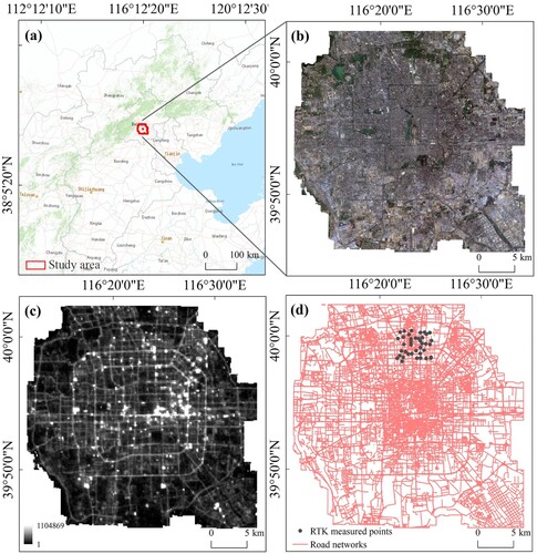
Beijing is the capital of China and is widely considered to be the nation’s economic, political, and cultural hub. As China has witnessed rapid urban sprawl, Beijing’s metropolitan area has become encircled by several ring roads. For this study, we focused on the urban core area (which covers roughly 850 km²) within the fifth ring road, as indicated in Figure 1(a). This area contains 276,722 buildings and 7,020 blocks. Using the LCZ classification scheme developed by Stewart and Oke (2012), we have identified 15 distinct LCZs in this region. We determined the LCZ through a combination of remote sensing data analysis, field observations, and expert knowledge. These include nine artificial LCZ types (such as compact high-rise, compact mid-rise, compact low-rise, and sparsely built), as well as six natural LCZ types that are characterized by minimal human intervention (such as dense trees, bushes or scrub, bare rock or pavement, and bodies of water).

Figure 1. Overview of the study area: (a) the geographic location of the study area; (b) ZY-3 true-color composited image; (c) Luojia-1 nighttime light image; and (d) road networks.

2.2. Data used

2.2.1. Remotely sensed data

In this study, we utilized daytime optical imagery and nighttime light data obtained from the ZY-3 and Luojia-1 satellites, respectively. Table 1 presents the specific parameters for these two satellites. Ziyuan-3 images used in our method incur additional costs, and as of 2019, the cumulative global effective coverage of the Ziyuan-3 satellite exceeds 79 million square kilometers; the three-line array stereo data has a domestic land coverage of 99.89% and a global coverage of over 63%. The ZY-3 satellite is a high-resolution, three-line array stereo mapping satellite that includes one multi-spectral camera with four spectral bands (red, green, blue, and near-infrared) and three multi-view panchromatic cameras that capture images from backward, nadir, and forward directions, respectively (details can be found in Figure S1). On 21 May, 2016, we obtained cloud-free multi-spectral and forward, backward, and nadir images. Additionally, we acquired two nadir images on 3 September, 2015, and 23 September, 2015. By fusing the multi-spectral and nadir panchromatic images, we were able to generate remote sensing images with a high spatial resolution of 2 m and excellent spectral quality. These images provided us with rich spectral information for accurately classifying land covers and LCZs (Zhao et al. 2021) (Figure 1(b)). Along-track and cross-track modes are two different acquisition configurations used in satellite imaging for capturing stereo pairs to generate multi-view point clouds. The difference between along-track and cross-track modes is the orientation and distribution of the captured images. Along-track mode provides broader coverage and perspective by capturing images in the anterior-posterior direction, while cross-track mode focuses on capturing images from adjacent nadir locations, emphasizing a more focused baseline in the nadir region. By combining along-track and cross-track modes, the generated multi-view point clouds benefit from the advantages of each configuration. This combined approach improves the accuracy and fidelity of the resulting point cloud data, allowing more detailed analysis and understanding of the urban structure and characteristics of the observed area.

Table 1. Satellite parameters of ZY-3 and Luojia-1 imageries (note that PAN refers to panchromatic and MS multi-spectral).

Parameter	ZY-3	Luojia-1
Launch time	09 January, 2012	02 June, 2018
Orbit altitude (km)	506	634
Swath width (km)	51 × 51	260 × 260
Spatial resolution (m)	PAN-nadir: 2.1 PAN-forward: 3.5 PAN-backward: 3.5 MS: 5.8 Pan-sharpened fusion: 2	130
Wavelength (nm)	PAN band: 500–800 Red band: 630–690 Green band: 520–590 Blue band: 450–520 Near-Infrared band: 770–890	480–800

The night light remote sensing images taken by the Luojia-1 satellite are released to a society free of charge. At present, the update range of Luojia-1 high-resolution night light data is limited and has not yet reached the global coverage level, and the coverage is wider in areas with a high density of night light (such as North America, Europe, East Asia, the Middle East, etc.). The Luojia-1 satellite is equipped with a high-sensitivity nightlight camera capable of producing images with an accuracy of 130 meters at ground resolution and a 260 km-wide nightlight imaging capability. This technology enables the accurate identification of roads and blocks (Ou et al. 2019). We used Luojia-1 NTL data collected in June, 2018 (Figure 1(c)).

2.2.2. Other auxiliary data

The other data include RTK-measured points, road networks, and LiDAR point clouds data. Easy-to-identify feature points were first selected on the ZY-3 pan-sharpened image. RTK points were intentionally selected and concentrated in the same place for image geometry correction and accuracy assessment. Then, the x, y, and z coordinate information of the ground control points were collected by field measurements. The field measurement technique used real-time kinematic (RTK) positioning technology. Each point was measured ten times, and the measurements were averaged. A total of 50 ground control points were collected; see Figure 1(d) for details. When processing the generated point clouds, ten control points were used to correct the images geometrically, and the remaining 40 control points were used to evaluate the geometric accuracy of the generated point clouds.

We obtained the road network data from the open street map (OSM) in November 2021(Figure 1(d)). We used the road networks to depict block boundaries and considered the blocks as the basic units of the LCZ mapping (Shin 2009; Zhao and Lü 2009). Since LCZs in blocks directly delineated by OSM can be heterogeneous and mixed, we further divided the mixed zones into purer sub-blocks for block attribute labeling (Vu et al. 2021; Zhang, Ghamisi, and Zhu 2019). We used several criteria and rules for delineation, such as spatial analysis, visual interpretation, land cover ratio, expert knowledge, and neighborhood analysis. The aim is to create more homogeneous sub-blocks in the mixed zone to facilitate accurate labeling of block attributes. Finally, 7020 zones were generated based on the road networks. The ground references of LCZs were manually interpreted based on field surveys by referring to open-source geographic information such as points of interest and street view images (Hu et al. 2021). The 7020 zones served as the spatial framework for the LCZ mapping and classification process, as well as accuracy assessment and data analysis.

LiDAR point clouds data in 2016 was collected from the A Leica ALS 60 system. DSM with 0.5 m resolution was created using the data. The LiDAR point clouds data was used to verify building roughness from ZY-3 multi-view point clouds data (Cao et al. 2020a). ZY-3 satellite imagery was used to generate point clouds data for building roughness estimation because ZY-3 satellite imagery provides extensive spatial coverage, allowing larger areas to be evaluated and described compared to other point clouds data sources. In addition, acquiring high-precision point cloud data from airborne LiDAR can involve higher costs and more challenges. In contrast, ZY-3 satellite imagery may provide a more readily available and cost-effective solution for generating point clouds data.

3. Methods

3.1. Overview of the classification approach

This study proposed a new LCZ classification approach that fully considers the advantages of diurnal satellite observations and multi-view (including along- and across-track modes) detections via synergistically using daytime ZY-3 stereo imageries and nighttime light data. Figure 2 provides the workflow of the classification procedure, which includes three key steps:

• Step 1: Land cover mapping

Figure 2. Proposed workflow of the LCZ mapping.

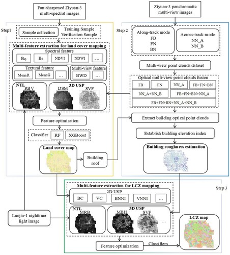
To improve land cover mapping, we proposed a method that utilizes multiple machine learning algorithms and features of underlying surfaces during both daytime and nighttime. Daytime features include spectral, textural, and multi-view features of pan-sharpened ZY-3 images, and 3D USPs. Nighttime features mainly employ nighttime light brightness data from the Luojia-1 satellite. Feature optimization was achieved using an average impurity reduction method. We selected the better performing classifier from two machine learning methods, namely RF and XGBoost algorithms, to perform the final land cover classification (Sanlang et al. 2021).

• Step 2: Building roughness estimation

By fully employing the ZY-3 satellite roll and camera inclination, both along- and across-track modes were adopted to generate multi-view point clouds. Based upon the fusion of multi-view point clouds, a building roughness estimation strategy proposed in our previous study was used to help LCZ mapping (Cao et al. 2020a). Specifically, the method includes the quality pre-judgment of point clouds, eliminating significant elevation bias between varying-view point clouds, and reconstructing building elevation through a cumulative index.

• Step 3: LCZ mapping

Based on the results of land covers and building roughness information, a new method regarding LCZ classification was introduced that integrates 2D USPs (e.g. building coverage, vegetation coverage, and nearest neighbor index (NNI)), 3D USPs (e.g. building roughness and sky view factor), and NTL data. Additionally, seven experiments were performed to assess the performance of different feature combinations. After that, the best-performing classifier was adopted for the final LCZ mapping.

3.2. Land cover mapping

3.2.1. Sample collection

The area network parity correction for ZY-3 panchromatic images and automatic alignment of the multi-spectral images was performed using ERDAS software. Then, the panchromatic nadir view image and multi-spectral image were fused to generate pan-sharpened photos with a 2-m spatial resolution. Based upon the spectral response of the ZY-3 pan-sharpened image features and field survey, five types of land covers were identified, including buildings, vegetation, soil, impervious surfaces, and water bodies. Table S2 provides details of the samples used for the different land covers. Eighty percent of the total samples were randomly chosen as training samples for the subsequent classification, and twenty percent of the samples were used for accuracy assessment.

3.2.2. Multi-feature extraction

Table 2 shows daytime and nighttime features obtained by diurnal satellite observations. The daytime features include spectral, textural, multi-view features, and 3D USPs. The nighttime feature can capture human activity intensities and be depicted by radiation brightness value (Zhang et al. 2018). Spectral features used varying satellite spectral bands (e.g. red, blue, green, and near-infrared bands), different vegetation indices [e.g. normalized difference vegetation index (NDVI), difference vegetation index (DVI), and ratio vegetation index (RVI)], normalized difference water index (NDWI), morphological building index (MBI), and morphological shadow index (MSI). Textural features chose eight Gray-Level Co-occurrence Matrix (GLCM) parameters, i.e. mean, variance, homogeneity, contrast, dissimilarity, entropy, angular second moment, and correlation (Haralick, Dinstein, and Shanmugam 1973; Xu et al. 2017). Multi-view images were also used for enhancing land cover mapping, including forward, backward, and nadir panchromatic bands. Additionally, three-dimensional USPs were chosen to represent height information, including the DSM and sky view factor (SVF). The DSM and SVF were calculated by the fusion of ZY-3 multi-view optical point clouds, and details can be found in Section 3.3.2.

Table 2. Multi-feature extraction for land cover mapping.

Category	Feature	Description/formula	References
Spectral feature	Spectral information	Red band (BR), green band (BG), blue band (BB), and near-infrared band (BNIR)	Faridatul and Wu (2018)
	Normalized Difference Vegetation Index (NDVI)	NDVI = (BNIR− BR)/ (BNIR + BR)	Jiang et al. (2006)
	Ratio Vegetation Index (RVI)	RVI = BNIR/BR	Priebe et al. (1999)
	Difference Vegetation Index (DVI)	DVI = BNIR − BR	Tucker (1979)
	Normalized Difference Water Index (NDWI)	NDWI = (BNIR− BG)/ (BNIR + BG)	McFeeters (1996)
	Morphological Building Index (MBI)	MBI was used to extract buildings by establishing the relationship between implicit features and morphological operators of facilities.	Huang and Zhang (2011)
	Morphological Shadow Index (MSI)	MSI is defined as a dual function of MBI, which highlights the shadow structure.	Huang and Zhang (2012)
Textural feature	Meani	The mean derived from GLCM (note that i refers to different spectral bands).	Huang and Wang (2019)
	Variancei	The variance was derived from GLCM.
	Homogeneityi	The homogeneity was derived from GLCM.
	Contrasti	The contrast was derived from GLCM.
	Dissimilarityi	The heterogeneity parameters were derived from GLCM.	Shaban and Dikshit (2001)
	Entropyi	The entropy was derived from GLCM.	Anys et al. (1998)
	Angular Second Momenti	The angular second moment was derived from GLCM.	Kim et al. (2011)
	Correlationi	The gray correlation was derived from GLCM.	Shafiq et al. (2015)
Multi-view feature	Nadir view (NAD)	A nadir panchromatic band resample to the spatial resolution of 2-m.	Huang et al. (2021)
	Forward view (FWD)	A forward panchromatic band resample to the spatial resolution of 2-m.
	Backward view (BWD)	A backward panchromatic band resamples to the spatial resolution of 2-m.
3D USP	Digital Surface Model (DSM)	The digital surface model is a ground elevation model that includes surface buildings, bridges, trees, etc.	Gomez, Hayakawa, and Obanawa (2015)
	Sky View Factor (SVF)	The sky view factor refers to the visible degree of the sky at the ground level. Its values vary from 0 to 1 and refer to the sky as not visible; in contrast, one refers to the evident atmosphere.	Zakšek, Oštir, and Kokalj (2011)
NTL	Radiation Brightness Value (RBV)	The radiation brightness value is the most intuitive feature of nighttime light images.	Huang et al. (2021)

3.2.3. Feature optimization

Feature optimization allows a better understanding of the importance of variables and is essential to improving classification accuracy. We used the gini index (GI), i.e. the average impurities reduction, to measure each variable’s importance (Strobl, Boulesteix, and Augustin 2007). The GI can be calculated based on the structure of the RF classifier and represents the average error reduction of each feature, which can be defined as (Zhang and Yang 2020): (1) $GI(P)=\sum _{k=1}^K{P}_k(1-P_k)=1-\sum _{k=1}^K{P}_k^2$(1) where GI (P) is the GI value, k denotes the k-th class, and P_k reflects the likelihood that the sample is from the k-th category. In general, a higher GI value means that the corresponding variable exerts a more significant influence on the classification.

3.2.4. Machine learning classifiers

Random Forest (RF) and XGBoost are popular machine learning algorithms that have been widely used for a variety of classification tasks, including LCZ classification (Huang et al. 2023).

There are a number of decision trees in the RF classifier, and all trees can be used to train samples and predict classification results (Breiman 2001). In addition, throughout computing the voting results in different decision trees, the classifier integrates voting results to predict the final classification results (Pal 2005). Existing literature has shown that the RF algorithm can significantly improve the classification results compared to individual decision trees. Meanwhile, the RF classifier performs well against outliers and noise, which can effectively avoid over-fitting (Yao et al. 2017). In addition, RF provides a measure of feature importance, which helps to understand the contribution of different variables in the classification task.

The XGBoost classifier refers to the eXtreme Gradient Boosting package. The classifier comprises the learning model, parameter tuning, and optimal objective function. The learning model combines essential functions and weights. Additionally, parameter tuning is necessary to build the model and optimize it. Notably, the correctness of the final learning model is determined by the goal function’s optimization degree. Thus, the better the optimization of the objective function is, the better the model generalization ability will be (Thongsuwan et al. 2021). It is optimized for speed and can efficiently handle large datasets.

Both RF and XGBoost have shown strong performance in classification tasks and have been widely adopted due to their ability to handle complex relationships, process large datasets, and provide robust and accurate predictions.

3.2.5. Accuracy evaluation

Classification post-processing is crucial for improving the final classification results (Stuckens, Coppin, and Bauer 2000). We built several classification post-processing rules according to Huang et al. (2017) (details can be found in Table S3). The accuracy assessment is an indispensable component of remotely sensed image classification, which provides an essential means for evaluating classification results. The confusion matrix was utilized to verify the land use classification (Lewis and Brown 2001). Four evaluation indices of the confusion matrix were employed in the study, including the Overall Accuracy (OA), kappa coefficient, User Accuracy (UA), and Producer Accuracy (PA).

3.3. Building roughness estimation

3.3.1. Generation of multi-view point clouds

To employ the advantages of satellite multi-view detections, various stereo pair schemes, including three along-track mode schemes, i.e. FB (forward + backward), FN (forward + nadir1), and BN (backward + nadir1), and two across-track mode schemes, including NN_A (nadir1 + nadir2) and NN_B (nadir2 + nadir3), were adopted to generate different optical point clouds. Table S4 provides different view panchromatic imageries used for stereo schemes. In particular, the rational polynomial model was utilized to characterize the linkage between image and ground spaces of the ZY-3 stereo pairs. Rational Polynomial Coefficients (RPCs) are warranted to drive the model and provided with the image by the supplier. Beyond this, ten in-situ RTK measurement points and automatic connection points were simultaneously employed in the rational function model error compensation to ensure model correction accuracy. After orientation parameter adjustment (i.e. removal of mismatched connection points), the exacted orientation of the stereo pairs was obtained (Xu, Xu, and Yang 2022). Image dense matching was performed using the enhanced Automatic Terrain Extraction (eATE) module (Cao et al. 2020a). The eATE can extract accurate, high-density elevation surfaces from overlapping images, which results in a higher density of points and more authentic characters.

3.3.2. Integration of multi-view point clouds

The stereo pairs used to generate point clouds feature different views and have different resolutions, camera tilt angles, satellite roll angles, and acquisition times. Thus, a quality pre-judgment of point clouds must be performed. In this study, the pre-judgment is primarily according to in-situ RTK observation data. We tested the associations between digital surface models generated by multi-view point clouds and 40 RTK in-situ measurements (Cao et al. 2020a). The ordinary least squares (OLS) regression model was performed to detect the accuracies of point clouds with different views. Upon examination, acceptable accuracies of point clouds were observed. Compared with the in-situ observations, the R² and root mean square error (RMSE) values of the stereo pairs of FB, FN, BN, NN_A, and NN_B were higher than 0.23 and lower than 5.02 m (details can be found in Figure S2). Therefore, those stereo pairs can be used for the subsequent point cloud fusion. Additionally, it is noteworthy that we employed DSM, generated by the fusion point cloud of FB, FN, BN, NN_A, and NN_B utilizing the interpolation algorithm, to enhance land cover mapping.

3.3.3. Building roughness estimation

Based on the results of multi-viewpoint cloud encryption and building labeling, we proposed a set of new cumulative elevation indexes to improve building roughness assessments. The index can estimate building elevation directly from point clouds, but those indices require enough elevation points (Cao et al. 2020a). Even though multi-view point cloud encryption was performed, some high-rise buildings may still have no or too few points. A threshold criterion was used to remove those buildings having few or no points. The strategy to determine the threshold value is a tradeoff between the number of buildings involved in the computing model and the accuracy with respect to building elevation estimations. Generally speaking, the accuracy in building roughness estimation increased with the threshold value rising. We established 12 sets of building indexes, i.e. maximum, minimum, mean, and cumulative indexes (from B10 to B90) within a specific building region. For the B70 index, it means that 70% of points in the building region are lower than the index value (Cao et al. 2020a). The calculation method is: (2) $B{P}_i=\{Poin{t}_{j}j=1,2,3,\dots ,n\}$(2) (3) $Poin{t}_j=\{x_j,y_j,z_j\}$(3) (4) $B{P}_i^{\mathrm{\prime }}=sor{t}_z(B{P}_i)$(4) (5) $Bk=z_{fix(n/10)\ast k+1}^{\mathrm{\prime }}$(5) where BP_i represents the matching points in the building i; sort_z function means the rank of the z value in the BP_i from high to low; an integer function is the fix function; the number of points in the building i is the value n. The estimated building elevation incorporated with DSM generated by point cloud fusion and accurate land cover information can be utilized to assess accurate building heights. In detail, the height information of above-ground objects (i.e. buildings) can be retrieved by removing terrain from the surface model via white top-hat reconstruction (Qin and Fang 2014).

3.4. LCZ mapping

3.4.1. Feature extraction

Table 3 provides the chosen features in LCZ classification. Three feature categories were used, including 2D USPs, 3D USPs, and NTL, to enhance LCZ mapping. Two-dimensional USPs mainly characterize landscape compositions and configurations. The compositions include building coverage (BC), vegetation coverage (VC), soil coverage (SC), impervious surface coverage (ISC), and water coverage (WC). Additionally, we employed the nearest neighbor index (NNI) to describe the configurations regarding different land covers. The NNI can effectively avoid the biases involved in LCZ classification, such as the same or similar landscape composition and 3D characteristics. Previous studies have proved that the NNI can precisely detect the spatial patterns of land covers (Diggle, Besag, and Gleaves 1976; Yang et al. 2013) and thus contribute to LCZ classification. Three typical spatial patterns concerning landscapes were adapted, namely, random distribution, aggregated distribution, and uniform distribution: (6) ${\overline{d}}_{min}={\displaystyle \frac{1}{n}\sum _{i=1}^n{d}_{min}}$(6) (7) $E(d_{min})={\displaystyle \frac{1}{2\sqrt{n/A}}}$(7) (8) $NNI={\displaystyle \frac{{\overline{d}}_{min}}{E(d_{min})}}$(8) where d_min is the minimum distance between a specific object (e.g. a building) and its identical objects, and $\overline{d}$_min is the average distance of minimum distances in the corresponding block. E(d_min) is the expected value of minimum distances in a completely spatially random pattern, which can be determined using the number of objects (n) and the block area (A). The spatial patterns can be identified as random, aggregated, and uniform distributions when the NNI values are equal to 1, lower than 1, and higher than 1, respectively.

Table 3. Multi-feature extraction for LCZ mapping.

Category	Feature	Description/formula	References
2D USP	Building coverage (BC)	The total building area is divided by the corresponding LCZ area.	Chen, Xu, and Devereux (2014)
	Vegetation coverage (VC)	The total vegetation area is divided by the corresponding LCZ area.	Cao et al. (2020b)
	Soil coverage (SC)	The total soil area is divided by the corresponding LCZ area.	Sanlang et al. (2021)
	Impervious surface coverage (ISC)	The total impervious surface coverage is divided by the corresponding LCZ area.	Homer et al. (2020)
	Water coverage (WC)	The total water area is divided by the corresponding LCZ area.	Sanlang et al. (2021)
	Building nearest neighbor index (BNNI)	The Nearest Neighbor Index (NNI) value of buildings.	Zhang, Du, and Wang (2018)
	Vegetation nearest neighbor index (VNNI)	The NNI value of vegetation.
	Soil nearest neighbor index (SNNI)	The NNI value of soil lands.
	Impervious nearest neighbor index (INNI)	The NNI value of impervious surfaces.
	Water nearest neighbor index (WNNI)	The NNI value of water bodies.
3D USP	Mean building height (MBH)	The average value of building heights in a LCZ unit.	Li et al. (2020)
	Mean building volume (MBV)	The average value of building volumes in a LCZ unit.
	Mean street width (MSW)	Average street width in a block unit.	Hermosilla et al. (2014)
	Sky view factor (SVF)	Sky view factor influenced by building.	Zakšek, Oštir, and Kokalj (2011)
	Canyon aspect ratio (CAR)	Average canyon height divided street width.	Chen, Xu, and Devereux (2014)
	Floor area ratio (FAR)	Total building area divided by block size.	Hermosilla et al. (2014)
	Frontal area index (FAI)	The frontal area divided the area of the block unit.	Kanda, Kawai, and Nakagawa (2005)
NTL	Mean radiation brightness (MRB)	Average brightness in a block unit.	Huang et al. (2021)

In addition, multiple 3D USPs were utilized to reveal vertical characteristics of each block that waits for classification, i.e. mean building height (MBH), mean building volume (MBV), mean street width (MSW), SVF, canyon aspect ratio (CAR), floor area ratio (FAR), and frontal area index (FAI). Since the LCZ scheme considers surface structures, covers, and human activities, nighttime light intensities, i.e. mean radiation brightness value (MRB), can help with LCZ mapping.

Based on spectral information from ZY-3 imagery and in-situ field surveys, we identified 15 LCZ types (Table S5) following Stewart and Oke (2012). The city block was employed as the primary division unit for LCZ classification, and it was generated by the road network data downloaded from OpenStreetMap. Moreover, our manual label result is highly consistent with the classified result from Quan (2019), suggesting the sample is reliable. Random sampling was used to divide the samples into 80% training and 20% validation datasets. Table S5 shows the 15 LCZ categories and the number of chosen training and verification samples. While sample size is important for training and evaluation of classification models, certain LCZ categories may have smaller sample sizes due to the characteristics of the study area and limitations in data availability. Efforts have been made to collect representative samples, but there is no guarantee that an equal number of samples will be available for each category. Two classifiers were utilized to label LCZ, including RF (Breiman 2001) and XGBoost (Thongsuwan et al. 2021) algorithms.

3.4.2. Experiment design

We determined the feature optimization using the GI method, and the best feature combination was chosen for the LCZ mapping. To further analyze the performance of daytime (i.e. 2D and 3D USPs) and nighttime features (i.e. NTL) on LCZ mapping, we designed seven experiments with different feature combinations based on feature optimization results (Table 4). We can assess each feature category’s impact on LCZ mapping. As shown, Exps. a, b, and c are designed to examine the ability of individual 2D USPs, 3D USPs, and nighttime light intensities in LCZ mapping. Exp. d includes fusion categories involving 2D and 3D USPs and is employed to determine the combined effect of 2D and 3D USPs on LCZ mapping. Exp. e selects 2D USPs and night light feature as input variables and can be utilized to verify the holistic effect of those features on LCZ classification. In addition, Exp. f uses 3D USPs and NTL features to perform the classification and can examine how 3D USPs and NTL interact to influence the classification effect. Exp. g consists of all categories.

Table 4. Experiments used for LCZ mapping.

Experiment	2D USP	3D USP	NTL
Exp. a	√
Exp. b		√
Exp. c			√
Exp. d	√	√
Exp. e	√		√
Exp. f		√	√
Exp. g	√	√	√

4. Results

4.1. Urban land cover mapping

4.1.1. Results of feature optimization

The Gini index-based importance ranking of the 48 selected variables in land cover classification is illustrated in Figure 3. The highest variable importance value was achieved by Mean_NIR (GI value = 0.099), followed by Band_NIR (GI value = 0.098), indicating the crucial roles of surface NIR spectral information and GLCM characteristics in land cover classification. As expected, 3D USPs demonstrated a significant influence on land cover classification (all GI values > 0.025), emphasizing their importance in land cover mapping. Spectral-related features exhibited a better classification performance (all GI values exceeded 0.010) compared to textural-related features (most GI values were below 0.010). In summary, the feature categories’ importance ranking, from high to low, were spectral features > 3D USPs > NTL > multi-view features > textural features.

Figure 3. Variable importance ranking for land cover mapping revealed by the RF algorithm.

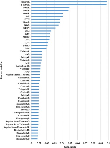
We conducted further tests to examine different OA values associated with varying input variables (details can be found in Figure S3). The OA value increased gradually with the increase in the number of input variables. The highest OA value (96.56%) was observed when 17 variables were selected as inputs. Therefore, we chose these 17 variables for subsequent land cover mapping. Detailed information on these 17 variables can be found in Table S6.

4.1.2. Results of land cover mapping

The classification accuracy of land cover using two classification algorithms, RF and XGBoost, is displayed in Table 5. The results show that the RF classifier had a higher overall accuracy (96.56%) compared to the XGBoost classifier (94.70%). The confusion matrices of land cover mapping using the RF and XGBoost classifiers are provided in Tables S7 and S8, respectively. Notably, the accuracy of soils and impervious ground using the XGBoost algorithm was considerably lower than that of the RF algorithm.

Table 5. Comparison of the performances of RF and XGBoost algorithms in land cover mapping. Note that the kappa coefficient, OA, PA, and UA represent a measure of classification accuracy, overall accuracy, producer’s accuracy, and user’s accuracy, respectively.

Category	RF (%)		XGBoost (%)
	PA	UA	PA	UA
Building	96.79	98.33	96.00	97.43
Vegetation	97.74	96.03	96.73	93.18
Soil	96.20	94.16	90.31	86.91
Impervious ground	94.14	93.69	88.76	90.97
Water	95.48	99.20	94.08	99.02
OA	96.56		94.70
Kappa coefficient	94.73		91.84

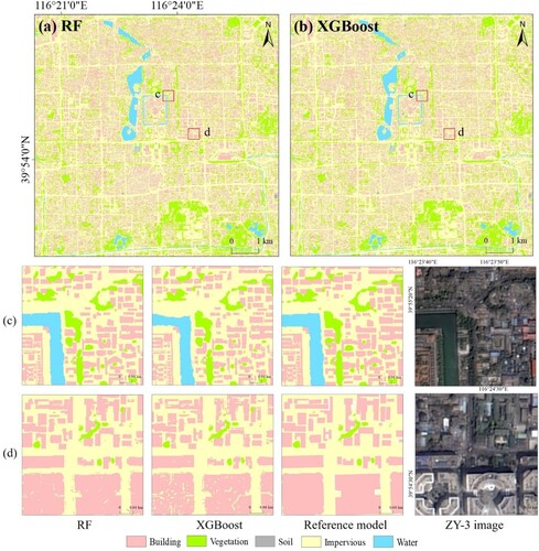
The details of land cover classification results by using RF and XGBoost classifiers are shown in Figure 4. As shown, the RF classifier can effectively identify buildings (Figure 4(c,d)). However, the XGBoost classifier failed to describe the buildings clearly, and some buildings were misclassified as impervious surfaces (Figure 4(c,d)). Possible reasons for these are the difficulty in identifying building roofs due to the variety of materials and a large number of artificial structures. The confusion was caused by the similar spectral information between building roofs and roads. Furthermore, for water detection, the performance of the RF algorithm was more acceptable than that of the XGBoost algorithm (Figure 4(c)), which shows that some water bodies were missing from the classification results. In addition, the XGBoost classifier identified slightly less vegetation than the RF algorithm.

Figure 4. Comparison of classification details by using the two classifiers: (a) RF classifier, (b) XGBoost classifier, (c) regions of interest c, (d) regions of interest d. Building outlines, vegetation information and water bodies, and human editing processes produced the comprehensive ‘reference model’.

4.2. Building roughness estimation

4.2.1. Characteristics of ZY-3 multi-view point clouds

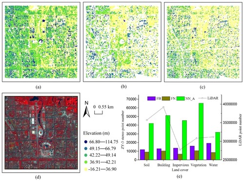
The characteristics of multi-view point clouds yielded by the across-track mode (i.e. NN_A) and along-track mode (i.e. FB and FN) are depicted in Figure 5. A significant difference in the point cloud distributions of NN_A, FB, and FN was observed. Among these, the point cloud produced by the across-track mode yielded the highest point number, indicating that the point cloud produced by the across-track mode may depict the roughness of underlying surfaces more accurately compared with that produced by the along-track mode. This is particularly true in building regions. Few numbers of FB and FN points in buildings were observed. The number of point clouds for FB, FN, NN_A, and LiDAR under varying land covers is presented in Figure 5(e). The number of NN_A points was considerably higher than that of FB and FN points. In addition, the LiDAR point cloud number ranking in different land covers was: buildings > soils > water > vegetation > impervious surfaces. However, the highest point cloud number in NN_A was vegetation, followed by buildings. It is noteworthy that the LCZ classification scheme fully considers 3D urban structures of underlying surfaces, which largely depends on the 3D characteristics of buildings and vegetation. Based upon this, it is vital to introduce ZY-3 across-track mode to enhance LCZ classification.

Figure 5. Characteristics of ZY-3 along- and across-track point clouds: (a) NN_A (nadir01 + nadir02), (b) FB (forward + backward), (c) FN (forward + nadir01), (d) false-color composite image, and (e) the number of multi-view point clouds in different land covers.

The spatial distribution of DSMs generated using different fusion schemes is shown in Figure S5. Different fused DSMs (with a spatial resolution of 2 m) were created using the interpolation algorithm (i.e. Triangulated Irregular Network) to demonstrate the effect of varying fused point clouds clearly. Among these, DSMs generated by single point clouds of the along-track (i.e. FB and FN) and across-track (i.e. NN_A) modes are illustrated in Figure S5a-S5c. The DSMs of fused point clouds produced by the along-track (i.e. FB + FN + BN) and across-track (i.e. NN_A + NN_B) modes are displayed in Figure S5d and S5e. The DSM generated by fused point clouds that integrate along- and across-track modes is shown in Figures S5f and S5g. The DSM result that did not use NN_B is provided in Figure S5f, while the DSM in Figure S5g used all point clouds generated by along- and across-track modes, i.e. FB + FN + BN + NN_A + NN_B. Clearer outlines of building areas in such DSMs produced by the across-track mode were observed, as shown in Figure S5h, compared to those using the along-track mode. Notably, building outlines in those DSMs constructed by the FB, FN, and FB + FN + BN point clouds were scarcely observable, probably because few optical points were created in building areas when using the along-track mode. Our observation indicates that the ability to depict buildings of the across-track mode point cloud is better than that of the along-track mode point cloud. However, the 3D characteristics of buildings and vegetation depend on both the quality and quantity of point clouds. The accuracy of along-track mode point clouds was observed to be slightly higher than that of the across-track mode point clouds (Figure S2). Therefore, blending the along- and across-track mode point cloud can be considered for the subsequent building roughness estimation.

4.2.2. Results of building roughness estimation

As stated earlier, building roughness estimation requires enough points. Even though fused point cloud was used to estimate roughness, some high-rise buildings posed no or few elevation points. It can significantly influence the accuracy of building elevation. Thus, a threshold-based method was introduced to remove buildings with no or few points. The threshold value used, the corresponding accuracy of building roughness estimation, and the remaining building number after performing the threshold method are presented in Table 6. Notably, R² and RMSE values were calculated based on the building elevations extracted from the ZY-3 and LiDAR point clouds. As shown, the R² and RMSE values increased as the threshold value rose. However, the number of estimated buildings decreased. It is vital to trade off the accuracy of roughness estimation and the number of estimated buildings. It was found that when the threshold value exceeded 5, the changes in R² and RMSE became stable. Therefore, buildings with a point number lower than or equal to five were excluded from the roughness estimation model.

Table 6. Changes in R² value, RMSE value, and building number under varying threshold settings.

Threshold value	R^2 value	RMSE value	Building number
0	0.12	20.79	3070
1	0.52	12.69	2972
2	0.56	11.92	2937
3	0.61	11.16	2904
4	0.65	10.37	2872
5	0.71	9.69	2844
6	0.72	9.22	2810
7	0.73	9.06	2782
8	0.75	8.70	2745
9	0.76	8.56	2727
10	0.76	8.43	2691

The associations between building elevations extracted from 12 building indexes and LiDAR point clouds are depicted in Figure S6. It is interesting to note that our observation suggests the mean elevation value of the ZY-3 point cloud was not the optimal solution (R² value = 0.72 and RMSE value = 9.22 m). As shown, the B70 index yielded the highest accuracy of the roughness estimation (R² value = 0.75 and RMSE value = 7.55 m), and the linear regression slope was closest to one (slope value = 0.96). In addition, upon examination, the performance of the B70 index was the best in different fused schemes, indicating that the B70 index did not depend on the stereo view and thus is suitable for the application concerning urban building elevation estimation.

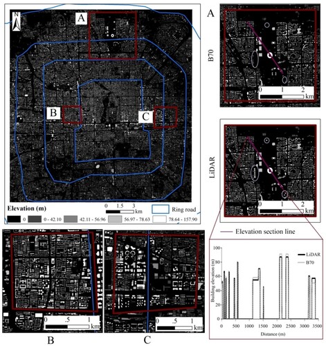
By integrating the above B70 index and multi-view point clouds, the building roughness in the core area of Beijing was computed. The estimated building roughness using the B70 index is illustrated in Figure 6. Notably, we extended and involved our roughness assessed model to a large scale that covers an area of approximately 850 km². A total of 276,722 buildings were calculated based on our model. As can be seen, the model results were pretty close to the building roughness estimated from the LiDAR point cloud. It illustrates the advantages of ZY-3 point cloud fusion and the great potential of high-resolution (2–6 m) stereo image data for urban 3D modeling in urban areas. In addition, the roughness of some high-rise buildings cannot be calculated because of insufficient elevation points.

Figure 6. Building roughness estimation.

4.3. LCZ mapping

4.3.1. Results of feature optimization

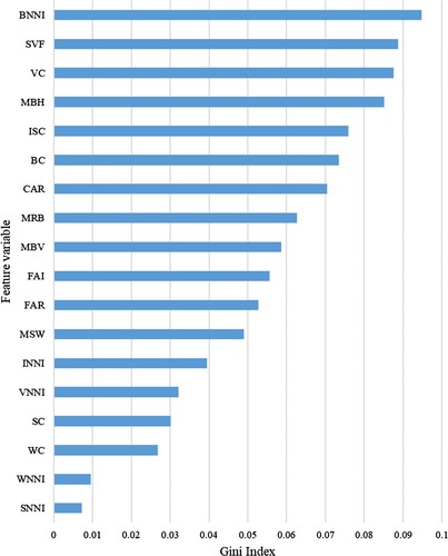
The variable importance ranking of the 18 variables in the LCZ mapping is presented in Figure 7. As shown, the most critical variable in LCZ mapping was BNNI, reaching the highest GI value of 0.095. The spatial pattern of the building occupied relatively high importance in LCZ mapping. In addition, SVF also had a high GI value of 0.089 and performed well in LCZ mapping, indicating the importance of 3D USPs in LCZ mapping (note that all GI values of 3D USPs were higher than 0.045). It was found that VC reached the third-highest GI value in LCZ (GI value = 0.088), indicating that vegetation coverage played a crucial role in LCZ classification. MRB was also vital to LCZ mapping, with a GI value of 0.063. In addition, other spatial patterns of land cover (i.e. INNI, VNNI, WNNI, and SNNI) occupied relatively low importance, and all of them had GI values below 0.04.

Figure 7. Variable importance ranking for LCZ mapping revealed by the RF algorithm.

We also tested the variable importance of features in different categories. The variable significance of 2D and 3D USPs is depicted in Figure S7. As shown, BNNI yielded the highest GI value of 0.24 in 2D USPs, suggesting that building spatial patterns is the most significant feature for LCZ mapping in 2D urban structures (Figure S7a). Vegetation and impervious surface coverage also had high GI values of 0.17 and 0.15. It suggests vegetation and impervious surface compositions are important to identify different LCZ settings. Additionally, it was found that, in 2D USPs, SNNI and WNNI (GI values < 0.02) showed relatively low variable importance, suggesting the spatial patterns of soil and water exert few influences on LCZ labeling. SVF (GI value = 0.24) is shown to substantially influence LCZ labeling in Figure S7b. Building height also yielded a high GI value of 0.14. It is noteworthy that all GI values for 3D USPs exceeded 0.11, indicating that 3D urban structures are essential for LCZ mapping.

To find the best feature combination and take into account the computational efficiency, we tested how the number of input variables influences the classification accuracy. The variation in overall accuracy (OA) values with different numbers of input variables is illustrated in Figure S8. As shown, the OA value significantly increased when variables changed from 1 to 6. The highest accuracy of 90.46% was observed when input variables were 16. Therefore, the optimal combination of 16 variables was selected to perform the LCZ mapping (details of the 16 optimal variables can be found in Table S9).

4.3.2. Results of LCZ mapping

The accuracy of the LCZ classification using RF and XGBoost classifiers is displayed in Table 7 (the confusion matrixes using two classifiers are shown in Tables S10 and S11). It was found that the RF classifier (the OA value = 90.46% and Kappa coefficient = 89.41) generated a high accuracy of LCZ mapping compared with the XGBoost classifier (the OA value = 88.82% and Kappa coefficient = 87.59). Notably, the PA values of LCZs 7 (lightweight low-rise), A/B (trees), and C (bush) using the RF algorithm reached 100%, which were significantly higher than those using the XGBoost algorithm. In addition, the UA values of LCZs 1 (compact high-rise), 3 (compact low-rise), 7 (lightweight low-rise), C (bush or scrub), and G (water) achieved 100% using the random forest classifier, considerably higher than those utilizing the XGBoost classifier. Our observations suggest that the RF classifier produced more accurate LCZ labeling results than the XGBoost classifier in terms of global and local perspectives.

Table 7. A comparison of using RF and XGBoost algorithms in LCZ mapping.

Category	RF (%)		XGBoost (%)
	PA	UA	PA	UA
1	89.47	100.00	89.47	94.44
2	83.67	95.35	79.59	95.12
3	81.82	100.00	78.79	96.30
4	93.58	91.62	91.44	88.60
5	93.55	93.05	94.62	89.80
6	84.13	86.89	80.95	87.93
7	100.00	100.00	84.62	84.62
8	88.24	83.33	85.29	80.56
9	90.59	86.52	88.24	86.21
A	100.00	89.83	86.79	88.46
C	100.00	100.00	90.00	81.82
D	93.88	90.20	93.88	92.00
E	95.33	86.81	93.46	86.06
F	82.89	88.73	85.53	86.67
G	85.29	100.00	88.24	100.00
OA	90.46		88.82
Kappa	89.41		87.59

The LCZ classification results by RF and XGBoost classifiers are detailed in Figure 8. Five enlargements of typical regions were chosen to demonstrate the disparities in the spatial specifics of different classification results. The misclassification of LCZ 8 (large low-rise) as LCZ 6 (open low-rise) in the red rectangle can be observed in Figure 8(c) when using the XGBoost classifier. However, the RF classifier correctly classified it as LCZ 8. It suggests that the RF classifier has more advantages in identifying impervious and pervious surfaces than the XGBoost classifier. In addition, as shown in Figure 8(c), LCZ 9 (sparse built), located in the red circle using the XGBoost classifier, was misclassified as LCZ E (bare rock or paved); in contrast, it was correctly labeled using the RF classifier.

Figure 8. Comparison of classification details by using the two classifiers. (a) RF classifier-study area, (b) XGBoost classifier-study area, (c) regions of interest c, (d) regions of interest d.

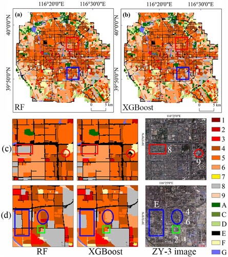
In particular, under a complicated urban environment setting (i.e. the blue rectangle in Figure 8(d)), the RF classifier effectively identified LCZ E (bare rock or paved), whereas the XGBoost classifier did not. It indicates that the RF classifier is more effective in LCZ classification under a highly complicated scene. It was found that LCZs 2 (compact mid-rise) and 4 (high-rise) (i.e. blue circle in Figure 8(d)) were correctly labeled using the RF classifier. However, they were wrongly labeled as LCZ 6 (open low-rise). It suggests that the RF classifier can effectively identify artificial structures with different vertical characteristics. In the green rectangle of Figure 8(d), it can be observed that the XGBoost classifier misclassified LCZ 6 (open low-rise) as LCZ 5 (open mid-rise). On the other hand, the RF classifier correctly labeled it as LCZ 6. It means the RF classifier exerts more advantages in distinguishing low-rise buildings from mid-rise ones.

5. Discussion

5.1. The advantages of using ZY-3 across-track model and satellite diurnal observations to help land cover mapping

Given that the fine-grained LCZ scheme considers land covers, 2D and 3D USPs, and human activities, it is vital to provide accurate land cover classification results for subsequent LCZ labeling. Existing literature has demonstrated that multi-view satellite observation (Liu et al. 2018) and nighttime anthropogenic light radiation data (Goldblatt et al. 2018) offer high potential in land cover mapping. Notably, in this study, we first utilized ZY-3 across-track mode to generate DSM and SVF to assist land cover classification. As stated earlier, point clouds generated by the across-track mode depicted the roughness of underlying surfaces more accurately than those produced by the along-track mode (Figure 5). We designed three experiments that verified how 3D USPs generated by across-track modes influence the land cover mapping results and how diurnal satellite observations help land cover mapping (Table 8, details of the confusion matrix can be found in Tables S12 and S13). It should be noted that Experiment #1 illustrated classification results that used 2D USPs (including spectral, textural, and multi-view features), 3D USPs (generated by along- and across-track modes), and NTL. Experiment #2 was similar to Experiment #1 but employed 3D USPs produced by single along-track mode. Compared with Experiment #1, Experiment #3 only considers daytime features, i.e. 2D and 3D USPs.

Table 8. Comparison of land cover classification accuracy using the RF classifier and different feature combinations.

Category	PA value (%)
	2D USP + 3D USP (produced by along- and across-track modes) + NTL (Experiment 1)	2D USP + 3D USP (produced by single along-track mode) + NTL (Experiment 2)	2D USP + 3D USP (produced by along- and across- track modes) (Experiment 3)
Building	96.79	90.81	93.66
Vegetation	97.74	93.52	93.01
Soil	96.20	93.09	90.97
Impervious surface	94.14	91.54	90.14
Water	95.48	92.68	92.06
OA	96.56	91.90	92.74
Kappa	94.73	87.65	88.87

It was found that the OA value of using fused 3D USPs increased by 4.66%, higher than that of using single along-track mode (Experiment #1 vs. #2, Table 8). Our finding is consistent with an investigation of the impacts of different features on land cover labels conducted by Al-Najjar et al. (2019), who found that accurate DSM can significantly improve the accuracy of land cover mapping. Also, all PA values of land covers increased using fused 3D USPs compared with those using 3D USPs generated by single along-track mode. Among these, the PA value of buildings increased by 5.98% and buildings yielded the most considerably improved accuracy when utilizing fused 3D USPs. It is probably because the synergetic use of along- and across-track modes to generate DSM and SVF can provide more accurate height information, and it is helpful to distinguish between building roofs and impervious surfaces (or soils) (Cao et al. 2020b). In addition, after adding the nighttime feature (i.e. NTL, Experiment #1 vs. #3), we found that the OA value increased by 3.82% (Goldblatt et al. 2018). All PA values of land covers increased after NTL was involved in the classification procedure. The highest increase was the PA value of soils (increased by 5.23%). The possible reason is that soils have the lowest night illumination compared with other underlying surfaces (Qiu et al. 2018). In addition, the PA value of impervious surfaces increased by 3.00%. It may be due to the most intimate relationship between impervious surface coverage and NTL (Huang et al. 2021; Sanlang et al. 2021).

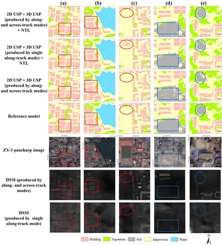
Figure 9 shows the spatial details of land cover classification utilizing different feature combinations. The best combination was observed to be 2D USP + 3D USP (produced by along- and across-track modes) + NTL (i.e. Experiment #1). As shown in Figure 9(a,b) red rectangles, some interior fragments in buildings were existed and incorrectly classified as impervious surfaces in Experiment #2 [i.e. 2D USP + 3D USP (produced by single along-track mode) + NTL], indicating that 3D USP produced by single along-track mode fails to completely and accurately capture buildings and is incapable of estimating accurate building roughness compared with that produced by along- and across-track modes. Meanwhile, some impervious surfaces in Figure 9(c) red circle were incorrectly classified as buildings, indicating the classification result by along-track 3D USPs easily confusing buildings and impervious grounds. All of these suggest the advantages of the use of point clouds produced by the across-track mode. Notably, we found that some soils were wrongly identified as impervious grounds using the feature combination without NTL, while they were correctly labeled utilizing NTL (Figure 9(c,d)). It suggests nighttime light observation can help the land cover classification in terms of distinguishing artificial and natural landscapes (Huang et al. 2021).

Figure 9. Three representative examples of classification details used 2D USP + 3D USP (produced by along- and across-track modes) + NTL, 2D USP + 3D USP (produced by single along-track mode) + NTL, and 2D USP + 3D USP (produced by along- and across-track modes).

5.2. The influence of different feature combinations on LCZ mapping

Notably, we conducted seven experiments to investigate the impact of satellite diurnal and multi-view observations on LCZ labeling accuracy (Table 4). Figure S10 presents a summary of the results obtained from different feature combinations, and the corresponding confusion matrices are shown in Table S14. The findings indicated that Exp. g, which integrated 2D and 3D USPs with NTL, achieved the highest classification accuracy with an OA value of 90.46%, while Exp. c, which solely utilized NTL, yielded the lowest OA value of 64.55%. The results also revealed that 2D USPs had a more significant impact on LCZ labeling than 3D USPs and NTL (e.g. Exps. a vs. b and Exps. a vs. c). The synergetic use of multiple feature combinations consistently generated higher classification accuracy than using a single feature class. For instance, Exp. d (OA value = 88.18%) outperformed Exp. a (OA value = 83.83%) by 4.35%, indicating that the combination of 2D and 3D USPs achieved a better result than using only 2D USPs. Similarly, Exp. e, which used 2D USPs and NTL, yielded a higher OA value (86.18%) than Exp. a. Furthermore, the use of 3D USPs significantly improved the PA values of LCZs 2, 3, 4, 5, 7, A, and C (Exp. e vs. g), which could not be accurately labeled using only 2D USPs and NTL due to similar spectral characteristics of buildings and vegetation with varying 3D structure parameters, making it difficult to distinguish between different types of buildings and vegetation using only 2D structure and NTL (Qiu et al. 2018; Quan 2019; Rosentreter, Hagensieker, and Waske 2020).

Additionally, the use of NTL data significantly increased the accuracy of LCZs E (bare rock or paved) and F (bare soil or sand) by 6.54% and 3.94%, respectively. This implies that NTL can be helpful in differentiating between natural and artificial LCZ categories, as well as in classifying LCZs 1-9, which have varying degrees of human activities. This finding is consistent with previous research (Goldblatt et al. 2018; Qiu et al. 2018) that has also demonstrated the usefulness of NTL in LCZ mapping.

Figure 10 shows classification results that employ 2D USPs, 3D USPs, and NTL yielded more accurate classification results than those using single 2D USPs. As shown in Scene 1, LCZ 2 (compact mid-rise), the red rectangular block, was misclassified as LCZ 5 (open mid-rise) when using single 2D USPs (i.e. Exp. a) and using 2D USPs and NTL (i.e. Exp. e). However, it was accurately identified when using single 2D USPs and 3D USPs (i.e. Exp. d) and using 2D USPs, 3D USPs, and NTL (i.e. Exp. g). The noteworthy difference between LCZs 2 and 5 is the building density, mean street width (MSW), and canyon aspect ratio (CAR). The mean street width of LCZ 5 is higher than that of LCZ 2, while the street aspect ratio of LCZ 5 is lower than that of LCZ 2. Roads can be classified as LCZ E (bare rock or paved). It was found that roads, the blue rectangular in Scene 1, were correctly identified as LCZ E in Exps. e and g when using NTL. Instead, some roads were misclassified in Exps. a and d, which did not use NTL. It suggests that high-resolution NTL data can assist in road identification. LCZ 8 (large low-rise), the red circle block, was correctly labeled using 2D USPs, 3D USPs, and NTL (Exp. g). However, it was wrongly labeled as LCZ 5 (open mid-rise) in Exps. a and e, which did not use 3D USPs. It suggests that 3D USPs can distinguish artificial LCZs with different building heights. Additionally, in Exp. d (without NTL), it was incorrectly identified as LCZ 3 (compact low-rise). The considerable difference between LCZs 3 and 5 is population densities, and thus NTL can be helpful in distinguishing between those two LCZ types.

Figure 10. Comparisons of the LCZ classification results of different experiments. Exp. a is the classification experiment without 3D USPs and NTL, Exps. d and e are the classification experiments without NTL and 3D USPs. Exp. g is the classification experiment using 3D USPs and NTL.

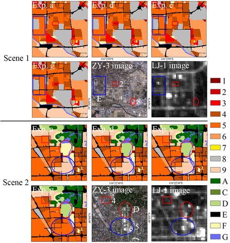
In Scene 2, LCZ 4 (open high-rise), the red rectangular block, was correctly classified using 3D USPs (i.e. Exps. d and g). Yet, it was wrongly labeled as LCZ 5 (open mid-rise) in Exps. a and e, which did not consider 3D USPs. It suggests that 3D USPs can help divide high-rise buildings from mid-rise ones. Additionally, in Exp. a, LCZ D (low plants), the red circle block, was mistakenly classified as LCZ F (bare soil or sand). However, in other experiments, it was correctly identified, showing that relying only on 2D USPs easily confuses low plants and bare soils. Our findings suggest the synergetic use of 2D USPs, 3D USPs, and NTL significantly improves the classification accuracy of LCZs.

5.3. Comparison with existing methods

In order to demonstrate the advantages of the proposed method, we compared it with existing approaches in terms of data sources, techniques, and accuracy (Table 9). Although different studies have used different accuracy validation strategies, validation samples, etc., we simply compare the overall accuracy obtained in different cases. Previous studies typically used mid-coarse resolution (e.g. 15–30 m) imageries for LCZ classification, which may not accurately capture 3D urban structure parameters and lead to low OA values (Brousse et al. 2016; Hay Chung, Xie, and Ren 2021; Fernandes et al. 2023; Huang et al. 2023). In contrast, our method utilized high-resolution (2–6 m) imageries and a building roughness estimation strategy based on the fusion of along- and across-track point clouds to improve LCZ mapping accuracy. Our method resulted in significantly higher PA values for LCZs 2, 3, 4, 5, 7, A, and C when compared to using 2D urban structure parameters alone (Figure S10), and higher OA value than most existing methods (Table 9). Additionally, visual features such as spectrums and textures, which are commonly used in preliminary image analysis (Voltersen et al. 2014), may not fully capture the complex urban scenes associated with LCZs. Our two-step procedure of first extracting land cover objects and then labeling LCZs helps to provide more discriminative features and significantly improves LCZ labeling accuracy by providing details of 2D and 3D urban structures. In conclusion, our proposed method offers a more accurate and cost-effective approach to LCZ mapping than existing methods.

Table 9. Comparisons of the existing methods for LCZ mapping.

Method	Data source	Study area	OA Value
LCZNet (Liu and Shi 2020)	Sentinel-2 multi-spectral data (10 m)	Greater Bay Area, Shanghai Metropolis, and Beijing Metropolis	88.61%
Supervised CNNs (Rosentreter, Hagensieker, and Waske 2020)	Multi-temporal Sentinel-2 composites	Eight German cities	86.50%
Semi-automatic algorithm (Chen, Zheng, and Hu 2020)	Landsat-8 remote sensing images (15 m), building data, and land use data	Chenzhou, China	69.54%
Canonical correlation forest (CCF) (Hu, Ghamisi, and Zhu 2018)	Sentinel-1 dual-pol data (10 m)	29 cities on a global scale	61.8%
Random forest classifier (Chen et al. 2021)	Sentinel-2 multispectral imagery and dual-polarized (HH + HV) PALSAR-2 data	Nanchang, China	89.96%
Residual convolutional neural Network (ResNet) (Qiu et al. 2018)	Sentinel-2 and Landsat-8 imagery, and the VIIRS-based NTL data	nine cities in Europe	78%
WUDAPT level 0 method (Wang et al. 2018)	Landsat-5 satellite images (30 m)	Hong Kong, China	58.00%
Proposed method	ZY-3 images 2.1 m resolution and Luojia-1 image 130 m resolution	Beijing, China	90.46%

Although the proposed LCZ mapping approach using multi-view of space and diurnal observations provides promising progress, there are still some limitations that can be addressed in future improvements. One limitation of the method may be the availability and accessibility of ZY-3 data. For example, the limited coverage or availability of ZY-3 images in certain regions may affect the generality and applicability of the algorithm. To address this limitation, future research could focus on expanding the dataset by incorporating data from other satellite sensors or exploring other data sources. In addition, the proposed approach focuses on the physical characteristics of urban areas and their relationship to the local climate environment. Future studies may consider the inclusion of socioeconomic and demographic data to further enhance the understanding of urban microclimate. By considering factors such as population density, land use patterns, and socioeconomic indicators, a more comprehensive analysis of LCZs and their impact on thermal comfort and urban planning can be achieved.

Another important aspect to consider is the transferability of the method to other geographic areas. While the method may perform well in the current research area, its effectiveness in different regions or under different environmental conditions may be uncertain. It is critical to discuss potential challenges and limitations when applying the method to other regions. To improve the transferability of the method, future research could investigate techniques such as domain adaptation or transfer learning. By incorporating data from multiple regions or domains in the training phase, the algorithm's ability to generalize to different regions can be improved. In addition, validation studies in different geographic environments can provide insight into the performance of the method and identify any specific limitations or areas for improvement. In summary, addressing limitations related to data accessibility, such as the availability of ZY-3 data and the inclusion of socioeconomic factors, and ensuring the transferability of the method across different regions are important considerations for future research.

6. Conclusions

In this work, we proposed a two-step method that uses high-resolution daytime ZY-3 stereo imageries and Luojia-1 nighttime light data for LCZ mapping. Firstly, fused 3D USPs produced by ZY-3 along- and across-track modes were used to enhance land cover mapping. In particular, the approach leverages multi-view point cloud encryption and building labeling to develop new cumulative elevation indexes that enhance building roughness assessments. Finally, 2D and 3D USPs were extracted for different land covers, and multi-classifiers were adopted to determine LCZ mapping. The conclusions can be drawn as follows.

1. The results show that the RF classifier had a higher overall accuracy (96.56%) compared to the XGBoost classifier (94.70%). All PA values of land covers increased using fused 3D USPs compared with those using 3D USPs generated by single along-track mode. Among these, the PA value of buildings increased by 5.98% and buildings yielded the most considerably improved accuracy when utilizing fused 3D USPs.

2. It was found that the RF classifier (the OA value = 90.46% and Kappa coefficient = 89.41) generated a high accuracy of LCZ mapping compared with the XGBoost classifier (the OA value = 88.82% and Kappa coefficient = 87.59). The OA value of LCZ mapping using 2D and 3D USPs (88.18%) achieved a better result than using only 2D USPs (83.83%). Additionally, the use of 3D USPs significantly improved the PA values of LCZs 2, 3, 4, 5, 7, A, and C. The use of NTL data significantly increased the accuracy of LCZs E (bare rock or paved) and F (bare soil or sand) by 6.54% and 3.94%, respectively.

In summary, our study provides a novel method for LCZ mapping that can enhance our understanding of urban microclimates and inform urban planning and design. The proposed approach can be applied to other regions and datasets, offering valuable insights for urban sustainability and climate resilience.

Acknowledgments

The author appreciates the editors and reviewers for their comments, suggestions, and valuable time and efforts in reviewing this manuscript.

Disclosure statement

No potential conflict of interest was reported by the author(s).

Data availability statement

The data that support the findings of this study are available from the corresponding author upon reasonable request. Data in this study can be available within the article or its supplementary materials.

Additional information

Funding

This work was supported by the National Natural Science Foundation of China [grant number: 41930650]; the Scientific Research Project of Beijing Municipal Education Commission [grant number: KM202110016004]; the Beijing Key Laboratory of Urban Spatial Information Engineering [grant number 20220111].

References

- Al-Najjar, H. A. H., B. Kalantar, B. Pradhan, V. Saeidi, A. A. Halin, N. Ueda, and S. Mansor. 2019. “Land Cover Classification from Fused DSM and UAV Images Using Convolutional Neural Networks.” Remote Sensing 11 (12): 1–18. https://doi.org/10.3390/rs11121461.
- Alberti, M., R. Weeks, and S. Coe. 2004. “Urban Land-Cover Change Analysis in Central Puget Sound.” Photogrammetric Engineering & Remote Sensing 70 (9): 1043–1052. https://doi.org/10.14358/PERS.70.9.1043.
- Anys, H., A. Bannari, D. C. He, and D. Morin. 1998. “Cartographie des Zones Urbaines a L'aide des Images Aeroportees MEIS-II” International Journal of Remote Sensing 19 (5): 883–894. https://doi.org/10.1080/014311698215775.
- Bechtel, B., P. J. Alexander, J. Böhner, J. Ching, O. Conrad, J. Feddema, G. Mills, L. See, and I. Stewart. 2015. “Mapping Local Climate Zones for a Worldwide Database of the Form and Function of Cities.” ISPRS International Journal of Geo-Information 4 (1): 199–219. https://doi.org/10.3390/ijgi4010199.
- Bechtel, B., and C. Daneke. 2012. “Classification of Local Climate Zones Based on Multiple Earth Observation Data.” IEEE Journal of Selected Topics in Applied Earth Observations and Remote Sensing 5 (4): 1191–1202. https://doi.org/10.1109/JSTARS.2012.2189873.
- Breiman, L. 2001. “Statistical Modeling: The Two Cultures (with Comments and a Rejoinder by the Author)” Statistical Science 16 (3): 199–215. https://doi.org/10.1214/ss/1009213726.
- Brousse, O., A. Martilli, M. Foley, G. Mills, and B. Bechtel. 2016. “WUDAPT, an Efficient Land Use Producing Data Tool for Mesoscale Models? Integration of Urban LCZ in WRF Over Madrid.” Urban Climate 17: 116–134. https://doi.org/10.1016/j.uclim.2016.04.001.
- Cao, S., Y. Cai, M. Du, Q. Weng, and L. Lu. 2022. “Seasonal and Diurnal Surface Urban Heat Islands in China: An Investigation of Driving Factors with Three-Dimensional Urban Morphological Parameters.” GIScience & Remote Sensing 59 (1): 1121–1142. https://doi.org/10.1080/15481603.2022.2100100.
- Cao, S., D. Hu, W. Zhao, M. Du, Y. Mo, and S. Chen. 2020a. “Integrating Multiview Optical Point Clouds and Multispectral Images from ZiYuan-3 Satellite Remote Sensing Data to Generate an Urban Digital Surface Model.” Journal of Applied Remote Sensing 14 (01): 1. https://doi.org/10.1117/1.jrs.14.014505.
- Cao, S., Q. Weng, M. Du, B. Li, R. Zhong, and Y. Mo. 2020b. “Multi-scale Three-Dimensional Detection of Urban Buildings Using Aerial LiDAR Data.” GIScience & Remote Sensing 57 (8): 1125–1143. https://doi.org/10.1080/15481603.2020.1847453.
- Castelo-Cabay, M., J. A. Piedra-Fernandez, and R. Ayala. 2022. “Deep Learning for Land Use and Land Cover Classification from the Ecuadorian Paramo.” International Journal of Digital Earth 15 (1): 1001–1017. https://doi.org/10.1080/17538947.2022.2088872.
- Chen, C., H. Bagan, X. Xie, Y. La, and Y. Yamagata. 2021. “Combination of Sentinel-2 and Palsar-2 for Local Climate Zone Classification: A Case Study of Nanchang, China.” Remote Sensing 13 (10): 1–21. https://doi.org/10.3390/rs13101902.
- Chen, Z., B. Xu, and B. Devereux. 2014. “Urban Landscape Pattern Analysis Based on 3D Landscape Models.” Applied Geography 55: 82–91. https://doi.org/10.1016/j.apgeog.2014.09.006.
- Chen, Y., B. Zheng, and Y. Hu. 2020. “Mapping Local Climate Zones Using arcGIS-Based Method and Exploring Land Surface Temperature Characteristics in Chenzhou, China.” Sustainability 12 (7). https://doi.org/10.3390/su12072974.
- Diggle, P. J., J. Besag, and J. T. Gleaves. 1976. “Statistical Analysis of Spatial Point Patterns by Means of Distance Methods.” Biometrics 32 (3): 659. https://doi.org/10.2307/2529754.
- Faridatul, M. I., and B. Wu. 2018. “Automatic Classification of Major Urban Land Covers Based on Novel Spectral Indices.” ISPRS International Journal of Geo-Information 7 (12). https://doi.org/10.3390/ijgi7120453.
- Fernandes, R., V. Nascimento, M. Freitas, and J. Ometto. 2023. “Local Climate Zones to Identify Surface Urban Heat Islands: A Systematic Review.” Remote Sensing 15 (4), https://doi.org/10.3390/rs15040884.
- Gál, T., B. Bechtel, and J. Unger. 2015. “Comparison of Two Different Local Climate Zone Mapping Methods.” ICUC9-9th International Conference on Urban Climates, Toulouse, France, July 20–24, 1–6.
- Goldblatt, R., M. F. Stuhlmacher, B. Tellman, N. Clinton, G. Hanson, M. Georgescu, C. Wang, et al. 2018. “Using Landsat and Nighttime Lights for Supervised Pixel-Based Image Classification of Urban Land Cover.” Remote Sensing of Environment 205: 253–275. https://doi.org/10.1016/j.rse.2017.11.026.
- Gomez, C., Y. Hayakawa, and H. Obanawa. 2015. “A Study of Japanese Landscapes Using Structure from Motion Derived DSMs and DEMs Based on Historical Aerial Photographs: New Opportunities for Vegetation Monitoring and Diachronic Geomorphology.” Geomorphology 242:11–20. https://doi.org/10.1016/j.geomorph.2015.02.021.
- Haralick, R.M., I.h. Dinstein, and K. Shanmugam. 1973. “Textural Features for Image Classification.” IEEE Transactions on Systems, Man, and Cybernetics SMC-3 (6): 610–621. https://doi.org/10.1109/TSMC.1973.4309314.
- Hay Chung, L. C., J. Xie, and C. Ren. 2021. “Improved Machine-Learning Mapping of Local Climate Zones in Metropolitan Areas Using Composite Earth Observation Data in Google Earth Engine.” Building and Environment 199:107879. https://doi.org/10.1016/j.buildenv.2021.107879.
- Hermosilla, T., J. Palomar-Vázquez, Á Balaguer-Beser, J. Balsa-Barreiro, and L. A. Ruiz. 2014. “Using Street Based Metrics to Characterize Urban Typologies.” Computers, Environment and Urban Systems 44:68–79. https://doi.org/10.1016/j.compenvurbsys.2013.12.002.
- Homer, C., J. Dewitz, S. Jin, G. Xian, C. Costello, P. Danielson, L. Gass, et al. 2020. “Conterminous United States Land Cover Change Patterns 2001–2016 from the 2016 National Land Cover Database.” ISPRS Journal of Photogrammetry and Remote Sensing 162:184–199. https://doi.org/10.1016/j.isprsjprs.2020.02.019.
- Hu, J., P. Ghamisi, and X. X. Zhu. 2018. “Feature Extraction and Selection of Sentinel-1 Dual-Pol Data for Global-Scale Local Climate Zone Classification.” ISPRS International Journal of Geo-Information 7 (9): 1–20. https://doi.org/10.3390/ijgi7090379.
- Hu, X., T. Li, T. Zhou, Y. Liu, and Y. Peng. 2021. “Contrastive Learning Based on Transformer for Hyperspectral Image Classification.” Applied Sciences (Switzerland) 11 (18). 8670. https://doi.org/10.3390/app11188670.
- Huang, F., S. Jiang, W. Zhan, B. Bechtel, Z. Liu, M. Demuzere, Y. Huang, et al. 2023. “Mapping Local Climate Zones for Cities: A Large Review.” Remote Sensing of Environment 292. https://doi.org/10.1016/j.rse.2023.113573.
- Huang, X., and Y. Wang. 2019. “Investigating the Effects of 3D Urban Morphology on the Surface Urban Heat Island Effect in Urban Functional Zones by Using High-Resolution Remote Sensing Data: A Case Study of Wuhan, Central China.” ISPRS Journal of Photogrammetry and Remote Sensing 152:119–131. https://doi.org/10.1016/j.isprsjprs.2019.04.010.
- Huang, X., D. Wen, J. Li, and R. Qin. 2017. “Multi-Level Monitoring of Subtle Urban Changes for the Megacities of China Using High-Resolution Multi-View Satellite Imagery.” Remote Sensing of Environment 196:56–75. https://doi.org/10.1016/j.rse.2017.05.001.
- Huang, X., J. Yang, J. Li, and D. Wen. 2021. “Urban Functional Zone Mapping by Integrating High Spatial Resolution Nighttime Light and Daytime Multi-View Imagery.” ISPRS Journal of Photogrammetry and Remote Sensing 175:403–415. https://doi.org/10.1016/j.isprsjprs.2021.03.019.
- Huang, X., and L. Zhang. 2011. “A Multidirectional and Multiscale Morphological Index for Automatic Building Extraction from Multispectral GeoEye-1 Imagery” Photogrammetric Engineering & Remote Sensing 77 (7): 721–732. https://doi.org/10.14358/PERS.77.7.721.
- Huang, X., and L. Zhang. 2012. “Morphological Building/Shadow Index for Building Extraction from High-Resolution Imagery Over Urban Areas.” IEEE Journal of Selected Topics in Applied Earth Observations and Remote Sensing 5 (1): 161–172. https://doi.org/10.1109/JSTARS.2011.2168195.
- Jiang, Z., A. R. Huete, J. Chen, Y. Chen, J. Li, G. Yan, and X. Zhang. 2006. “Analysis of NDVI and Scaled Difference Vegetation Index Retrievals of Vegetation Fraction.” Remote Sensing of Environment 101 (3): 366–378. https://doi.org/10.1016/j.rse.2006.01.003.
- Kamali Maskooni, E., H. Hashemi, R. Berndtsson, P. Daneshkar Arasteh, and M. Kazemi. 2021. “Impact of Spatiotemporal Land-Use and Land-Cover Changes on Surface Urban Heat Islands in a Semiarid Region Using Landsat Data.” International Journal of Digital Earth 14 (2): 250–270. https://doi.org/10.1080/17538947.2020.1813210.
- Kanda, M., T. Kawai, and K. Nakagawa. 2005. “A Simple Theoretical Radiation Scheme for Regular Building Arrays.” Boundary-Layer Meteorology 114 (1): 71–90. https://doi.org/10.1007/s10546-004-8662-4.
- Kane, K., J. Tuccillo, A. M. York, L. Gentile, and Y. Ouyang. 2014. “A Spatio-Temporal View of Historical Growth in Phoenix, Arizona, USA.” Landscape and Urban Planning 121:70–80. https://doi.org/10.1016/j.landurbplan.2013.08.011.
- Kim, M., T. A. Warner, M. Madden, and D. S. Atkinson. 2011. “Multi-Scale GEOBIA with Very High Spatial Resolution Digital Aerial Imagery: Scale, Texture and Image Objects.” International Journal of Remote Sensing 32 (10): 2825–2850. https://doi.org/10.1080/01431161003745608.
- Lee, Y. Y., M. F. Md Din, M. Ponraj, Z. Z. Noor, K. Iwao, and S. Chelliapan. 2017. “Overview of Urban Heat Island (UHI) Phenomenon Towards Human Thermal Comfort.” Environmental Engineering and Management Journal 16 (9): 2097–2112. https://doi.org/10.30638/eemj.2017.217.
- Lewis, H.G., and M. Brown. 2001. “A Generalized Confusion Matrix for Assessing Area Estimates from Remotely Sensed Data.” International Journal of Remote Sensing 22 (16): 3223–3235. https://doi.org/10.1080/01431160152558332.
- Li, M., E. Koks, H. Taubenböck, and J. van Vliet. 2020. “Continental-Scale Mapping and Analysis of 3D Building Structure.” Remote Sensing of Environment 245:111859. https://doi.org/10.1016/j.rse.2020.111859.
- Liu, T., A. Abd-Elrahman, A. Zare, B. A. Dewitt, L. Flory, and S. E. Smith. 2018. “A Fully Learnable Context-Driven Object-Based Model for Mapping Land Cover Using Multi-View Data from Unmanned Aircraft Systems.” Remote Sensing of Environment 216:328–344. https://doi.org/10.1016/j.rse.2018.06.031.
- Liu, S., and Q. Shi. 2020. “Local Climate Zone Mapping as Remote Sensing Scene Classification Using Deep Learning: A Case Study of Metropolitan China.” ISPRS Journal of Photogrammetry and Remote Sensing 164:229–242. https://doi.org/10.1016/j.isprsjprs.2020.04.008.
- McFeeters, S. K. 1996. “The Use of the Normalized Difference Water Index (NDWI) in the Delineation of Open Water Features.” International Journal of Remote Sensing 17 (7): 1425–1432. https://doi.org/10.1080/01431169608948714.
- Mills, G., B. Bechtel, J. Ching, L. See, J. Feddema, M. Foley, P. Alexander, and M. O’Connor. 2015. “An Introduction to the WUDAPT Project.” Proceedings of the 9th International Conference on Urban Climate (ICUC9), 6.
- Ou, J., X. Liu, P. Liu, and X. Liu. 2019. “Evaluation of Luojia 1-01 Nighttime Light Imagery for Impervious Surface Detection: A Comparison with NPP-VIIRS Nighttime Light Data.” International Journal of Applied Earth Observation and Geoinformation 81:1–12. https://doi.org/10.1016/j.jag.2019.04.017.
- Owers, C. J., R. M. Lucas, D. Clewley, B. Tissott, S. M. T. Chua, G. Hunt, N. Mueller, et al. 2022. “Operational Continental-Scale Land Cover Mapping of Australia Using the Open Data Cube.” International Journal of Digital Earth 15 (1): 1715–1737. https://doi.org/10.1080/17538947.2022.2130461.
- Pal, M. 2005. “Random Forest Classifier for Remote Sensing Classification.” International Journal of Remote Sensing 26 (1): 217–222. https://doi.org/10.1080/01431160412331269698.
- Priebe, S., P. Huxley, S. Knight, and S.E. Summary. 1999. “Application and Results of the Manchester Short Assessment of Quality of Life (Mansa) Background Based on Experiences and Empirical Evidence Gained in Studies Using the Lancashire Quality of Life Profile (LQLP), the Manchester Short.” 7–12.
- Qin, R., and W. Fang. 2014. “A Hierarchical Building Detection Method for Very High Resolution Remotely Sensed Images Combined with DSM Using Graph cut Optimization.” Photogrammetric Engineering & Remote Sensing 80 (9): 873–883. https://doi.org/10.14358/PERS.80.9.873.
- Qiu, C., M. Schmitt, L. Mou, P. Ghamisi, and X. X. Zhu. 2018. “Feature Importance Analysis for Local Climate Zone Classification Using a Residual Convolutional Neural Network with Multi-Source Datasets.” Remote Sensing 10 (10): 1–14. https://doi.org/10.3390/rs10101572.
- Quan, J. L. 2019. “Enhanced Geographic Information System-Based Mapping of Local Climate Zones in Beijing, China.” Science China Technological Sciences 62 (12): 2243–2260. https://doi.org/10.1007/s11431-018-9417-6.
- Rosentreter, J., R. Hagensieker, and B. Waske. 2020. “Towards Large-Scale Mapping of Local Climate Zones Using Multitemporal Sentinel 2 Data and Convolutional Neural Networks.” Remote Sensing of Environment 237:111472. https://doi.org/10.1016/j.rse.2019.111472.
- Sanlang, S., S. Cao, M. Du, Y. Mo, Q. Chen, and W. He. 2021. “Integrating Aerial Lidar and Very-High-Resolution Images for Urban Functional Zone Mapping.” Remote Sensing 13 (13). https://doi.org/10.3390/rs13132573.
- Shaban, M. A., and O. Dikshit. 2001. “Improvement of Classification in Urban Areas by the Use of Textural Features: The Case Study of Lucknow City, Uttar Pradesh.” International Journal of Remote Sensing 22 (4): 565–593. https://doi.org/10.1080/01431160050505865.
- Shafiq, M. A., Z. Wang, A. Amin, T. Hegazy, M. Deriche, and G. AlRegib. 2015. “Detection of Salt-Dome Boundary Surfaces in Migrated Seismic Volumes Using Gradient of Textures.” SEG Technical Program Expanded Abstracts 34:1811–1815. https://doi.org/10.1190/segam2015-5927230.1.
- Shin, H. B. 2009. “Residential Redevelopment and the Entrepreneurial Local State: The Implications of Beijing's Shifting Emphasis on Urban Redevelopment Policies.” Urban Studies 46 (13): 2815–2839. https://doi.org/10.1177/0042098009345540.
- Stewart, I. D. 2011. “A Systematic Review and Scientific Critique of Methodology in Modern Urban Heat Island Literature.” International Journal of Climatology 31 (2): 200–217. https://doi.org/10.1002/joc.2141.
- Stewart, I. D., and T. R. Oke. 2012. “Local Climate Zones for Urban Temperature Studies.” Bulletin of the American Meteorological Society 93 (12): 1879–1900. https://doi.org/10.1175/BAMS-D-11-00019.1.
- Strobl, C., A. L. Boulesteix, and T. Augustin. 2007. “Unbiased Split Selection for Classification Trees Based on the Gini Index.” Computational Statistics & Data Analysis 52 (1): 483–501. https://doi.org/10.1016/j.csda.2006.12.030.
- Stuckens, J., P. R. Coppin, and M. E. Bauer. 2000. “Integrating Contextual Information with Per-Pixel Classification for Improved Land Cover Classification.” Remote Sensing of Environment 71 (3): 282–296. https://doi.org/10.1016/S0034-4257(99)00083-8.
- Thongsuwan, S., S. Jaiyen, A. Padcharoen, and P. Agarwal. 2021. “ConvXGB: A New Deep Learning Model for Classification Problems Based on CNN and XGBoost.” Nuclear Engineering and Technology 53 (2): 522–531. https://doi.org/10.1016/j.net.2020.04.008.
- Tucker, C.J. 1979. “Red and Photographic Infrared Linear Combinations for Monitoring Vegetation.” Remote Sensing of Environment 8 (2): 127–150. https://doi.org/10.1016/0034-4257(79)90013-0.
- United Nations, Department of Economic and Social Affairs, Population Division. 2018. World Urbanizatior Prospects: The 2018 Revision, Methodology. Working Paper No, ESA/P/WP.252. New York: United Nations.
- Voltersen, M., C. Berger, S. Hese, and C. Schmullius. 2014. “Object-Based Land Cover Mapping and Comprehensive Feature Calculation for an Automated Derivation of Urban Structure Types at Block Level.” Remote Sensing of Environment 154:192–201. https://doi.org/10.1016/j.rse.2014.08.024.
- Voogt, J. A., and T. R. Oke. 2003. “Thermal Remote Sensing of Urban Climates.” Remote Sensing of Environment 86 (3): 370–384. https://doi.org/10.1016/S0034-4257(03)00079-8.
- Vu, T. T., N. V. A. Vu, H. P. Phung, and L. D. Nguyen. 2021. “Enhanced Urban Functional Land Use Map with Free and Open-Source Data.” International Journal of Digital Earth 14 (11): 1744–1757. https://doi.org/10.1080/17538947.2021.1970262.
- Wang, R., C. Ren, Y. Xu, K. K. L. Lau, and Y. Shi. 2018. “Mapping the Local Climate Zones of Urban Areas by GIS-Based and WUDAPT Methods: A Case Study of Hong Kong.” Urban Climate 24:567–576. https://doi.org/10.1016/j.uclim.2017.10.001.
- Xiao, J., Y. Shen, J. Ge, R. Tateishi, C. Tang, Y. Liang, and Z. Huang. 2006. “Evaluating Urban Expansion and Land Use Change in Shijiazhuang, China, by Using GIS and Remote Sensing.” Landscape and Urban Planning 75 (1-2): 69–80. https://doi.org/10.1016/j.landurbplan.2004.12.005.
- Xu, Y., C. Ren, M. Cai, N. Y. Y. Edward, and T. Wu. 2017. “Classification of Local Climate Zones Using ASTER and Landsat Data for High-Density Cities.” IEEE Journal of Selected Topics in Applied Earth Observations and Remote Sensing 10 (7): 3397–3405. https://doi.org/10.1109/JSTARS.2017.2683484.
- Xu, E., Z. Xu, and K. Yang. 2022. “Using 2-Lines Congruent Sets for Coarse Registration of Terrestrial Point Clouds in Urban Scenes.” IEEE Transactions on Geoscience and Remote Sensing 60:1–18. https://doi.org/10.1109/TGRS.2021.3128403.
- Yang, G., R. Pu, J. Zhang, C. Zhao, H. Feng, and J. Wang. 2013. “Remote Sensing of Seasonal Variability of Fractional Vegetation Cover and Its Object-Based Spatial Pattern Analysis Over Mountain Areas.” ISPRS Journal of Photogrammetry and Remote Sensing 77:79–93. https://doi.org/10.1016/j.isprsjprs.2012.11.008.
- Yang, J., Y. Wang, C. Xiu, X. Xiao, J. Xia, and C. Jin. 2020. “Optimizing Local Climate Zones to Mitigate Urban Heat Island Effect in Human Settlements.” Journal of Cleaner Production 275:123767. https://doi.org/10.1016/j.jclepro.2020.123767.
- Yao, Y., X. Li, X. Liu, P. Liu, Z. Liang, J. Zhang, and K. Mai. 2017. “Sensing Spatial Distribution of Urban Land Use by Integrating Points-of-Interest and Google Word2Vec Model.” International Journal of Geographical Information Science 31 (4): 825–848. https://doi.org/10.1080/13658816.2016.1244608.
- Zakšek, K., K. Oštir, and Ž. Kokalj. 2011. “Sky-View Factor as a Relief Visualization Technique.” Remote Sensing 3 (2): 398–415. https://doi.org/10.3390/rs3020398.
- Zhang, X., S. Du, and Q. Wang. 2018. “Integrating Bottom-up Classification and Top-Down Feedback for Improving Urban Land-Cover and Functional-Zone Mapping.” Remote Sensing of Environment 212:231–248. https://doi.org/10.1016/j.rse.2018.05.006.
- Zhang, G., P. Ghamisi, and X. X. Zhu. 2019. “Fusion of Heterogeneous Earth Observation Data for the Classification of Local Climate Zones.” IEEE Transactions on Geoscience and Remote Sensing 57 (10): 7623–7642. https://doi.org/10.1109/TGRS.2019.2914967.
- Zhang, R., C. Huang, X. Zhan, H. Jin, and X. P. Song. 2018. “Development of S-NPP VIIRS Global Surface Type Classification map Using Support Vector Machines.” International Journal of Digital Earth 11 (2): 212–232. https://doi.org/10.1080/17538947.2017.1315462.
- Zhang, F., and X. Yang. 2020. “Improving Land Cover Classification in an Urbanized Coastal Area by Random Forests: The Role of Variable Selection.” Remote Sensing of Environment 251:112105. https://doi.org/10.1016/j.rse.2020.112105.
- Zhao, S., X. Jiang, G. Li, Y. Chen, and D. Lu. 2021. “Integration of ZiYuan-3 Multispectral and Stereo Imagery for Mapping Urban Vegetation Using the Hierarchy-Based Classifier.” International Journal of Applied Earth Observation and Geoinformation 105:102594. https://doi.org/10.1016/j.jag.2021.102594.
- Zhao, P., and B. Lü. 2009. “Transportation Implications of Metropolitan Spatial Planning in Mega-City Beijing.” International Development Planning Review 31 (3): 235–261. https://doi.org/10.3828/idpr.31.3.2.