Modification and validation of a new method to improve the accuracy of MODIS-derived dew point temperature over mainland China

ABSTRACT

MODIS atmospheric profile products (MOD07_L2 and MYD07_L2) have been widely used for near-surface dew point temperature ($T_d$) estimation. However, their accuracy over large scale has seldom been evaluated. In this study, we validated these two products comprehensively against 2153 stations over mainland China. MOD07_L2 was suggested by our study because it achieved higher accuracy in either of two frequently-used methods. To be specific, the root-mean-square error (RMSE) achieved by MOD07_L2 and MYD07_L2 was 5.82 and 7.42 °C, respectively. On this basis, a recent ground-based correction method was modified to further improve their accuracy. Our focus is to investigate whether this ground-based approach is applicable to large-scale remote sensing applications. The results show that this new method showed great potential for $T_d$ estimation independently from ground observations. Through the introduction of MODIS land surface products, the RMSE it achieved for MOD07_L2 and MYD07_L2 was 5.23 and 5.59 °C, respectively. Further analysis shows that it was particularly useful in capturing the annual average $T_d$ patterns. The R², RMSE, and bias of annual average daily mean $T_d$ estimates were 0.95, 1.84 °C, and 0.53 °C, and those achieved for annual average instantaneous $T_d$ estimates were 0.94, 2.09 °C, and 0.75 °C, respectively.

KEYWORDS:

• Dew point temperature
• relative humidity
• atmospheric profiles
• MODIS
• remote sensing

1. Introduction

Dew point temperature ($T_d$) is the temperature to which the air must be cooled to become saturated with water vapor given that the air pressure and water vapor remain constant (Merva 1975; Shank, Hoogenboom, and McClendon 2008). As a direct indicator of near-surface humidity, $T_d$ is one of the most important climatic variables controlling many biological and physical processes between the hydrosphere, atmosphere and biosphere (Ali, Fowler, and Mishra 2018; Dou et al. 2021; Pumo and Noto 2021). Consequently, accurate near-surface $T_d$ monitoring is vital for a wide range of applications such as agriculture production (Yue, Yang, and Wang 2022), terrestrial hydrology and ecology (Bello, Mailhot, and Paquin 2021; Wu et al. 2022), climate and environment change (Denson, Wasko, and Pee 2021; Sein, Ullah, and Iyakaremye 2022), public health (Iyakaremye et al. 2021; Ullah et al. 2022), and disease vectors propagating (Chen et al. 2022; Masoumi, van Genderen, and Mesgari 2020). In general, $T_d$ with high accuracy can be calculated easily from ground-based air temperature ($T_a$) and relative humidity (RH) observations. However, these observations measured as point samples have limited ability in reflecting the spatial heterogeneity of $T_d$ (Hashimoto et al. 2008; Ritter, Berkelhammer, and Beysens 2019; You et al. 2015). In contrast, reanalysis products provide continuous $T_d$ estimation with global coverage by combining models with observations, but their spatial resolution is usually too low for many local applications (Berg et al. 2003; Viggiano et al. 2021; Wang and Yuan 2022). There exists a key niche for $T_d$ information with fine resolution, because many hydrological, climatological, and ecological models seek to describe processes at scales of 1∼10 km (Famiglietti et al. 2018; Ji et al. 2023; Razafimaharo et al. 2020; Turner, Ollinger, and Kimball 2004; Wood et al. 2011; Zhu, Jia, and Lű 2017a).

Moderate Resolution Imaging Spectroradiometer (MODIS), provides an unprecedented global coverage of critical land surface and atmosphere parameters, which is a potentially valuable alternative to characterize fine-resolution $T_d$ patterns across large areas. This is particularly true for MOD07 Level-2 atmospheric profile product because it provides temperature and moisture profiles distributed at 20 vertical levels with 5 km pixel resolution (King et al. 2003; Sobrino et al. 2015). Consequently, the need for $T_d$ information with fine resolution has resulted in numerous studies looking into MOD07 product to meet this requirement (Hwang and Choi 2013; Jiao et al. 2015; Liu et al. 2021; Ryu et al. 2011; Zhu, Wang, and Jia 2023). According to these studies, depending on the vertical levels used, two approaches may be distinguished in the retrieval of near-surface $T_d$ from MOD07 product (Zhang et al. 2014). The first approach extracts $T_d$ at the lowest vertical pressure level as the surrogate for near-surface $T_d$ directly. For example, in the net radiation model developed by Bisht et al. (2005) and the evapotranspiration model developed by Venturini, Rodriguez, and Bisht (2011), $T_d$ at the pressure level of 1000 hPa from MOD07_L2 product was adopted as the representation of near-surface $T_d$ over the Southern Great Plains region in the USA. The second approach interpolates $T_d$ at the two lowest pressure levels to near-surface level based on the hydrostatic assumption (Bisht and Bras 2010; Famiglietti et al. 2018; Kim and Hogue 2008; Liu et al. 2021; Tang and Zhao 2008; Verma et al. 2016). Although both these two approaches have been adopted widely at regional scale, their accuracy over large scale has seldom been validated robustly, making the quality of $T_d$ retrieval in many modeling applications heretofore relatively unknown. Given this background, the accuracy of the second approach for global $T_d$ estimation was validated by Famiglietti et al. (2018) based on 109 ground meteorological stations. Their results suggest that further studies are required to improve the accuracy of $T_d$ retrieval from MODIS products.

For this purpose, we first tried to seek approaches from studies that are performed based on other satellite sensors. However, due to the lack of atmospheric profiles, few studies have been conducted to retrieve near-surface $T_d$ from other satellite observations. Fortunately, a large number of studies have been performed for near-surface $T_d$ estimation based on in-situ meteorological observations. Apart from those conducted on the basis of machine learning models such as Baghban et al. (2016), Park et al. (2021), Dong et al. (2022) and Qiu et al. (2022), a major assumption of these studies is that near-surface $T_d$ can be approximately estimated from daily minimum air temperature ($T_{amin}$). For example, in the early studies of Allen et al. (1998) and Mu et al. (2009), near-surface $T_d$ was assumed to be equivalent to $T_{amin}$ for the development of evapotranspiration models. Further studies show that this assumption generally holds for boreal and arctic regions under nonfrozen conditions, but leads to relatively large errors in warmer, drier climate conditions (Dong et al. 2022; Mahmood and Hubbard 2005; Paredes and Pereira 2019; Todorovic, Karic, and Pereira 2013). As a result, a variety of correction methods have been proposed subsequently to estimate $T_d$ accurately from $T_{amin}$. A review of these methods is available in Paredes et al. (2020) and Qiu et al. (2022). These $T_{amin}$-based correction methods at site scale have enlightening significance for the retrieval of near-surface $T_d$ from MODIS products, because numerous studies confirm that $T_{amin}$ estimates with high accuracy can be achieved by adopting MODIS nighttime land surface temperature ($T_s$) as proxy (Chen et al. 2021; Lin et al. 2012; Oyler et al. 2016; Shiff, Helman, and Lensky 2021; Vancutsem et al. 2010; Zhu, Lű, and Jia 2013).

Inspired by these studies, the main objective of our work is to perform a comprehensive validation of MODIS atmospheric profile products for the retrieval of near-surface $T_d$ and further improve their accuracy through the combination with MODIS land surface products. The validation was conducted using hourly observations from 2153 meteorological stations across mainland China. Although a similar validation has been performed at global scale in Famiglietti et al. (2018), they only evaluated the accuracy of MOD07_L2 product with hypsometric interpolation method based on 109 meteorological stations. In contrast, the evaluation in this study was conducted for both MOD07_L2 and MYD07_L2 products. In addition to hypsometric interpolation method, we also evaluated the validity of $T_d$ retrieved at the lowest vertical pressure level as the surrogate for near-surface $T_d$. The improvement was achieved based on the correction method proposed by Qiu et al. (2021). The difference is that the original Qiu et al. (2021) was performed to estimate daily average $T_d$ on the basis of meteorological observations, while the focus of our research is to investigate whether this ground-based approach is applicable to large-scale remote sensing applications for both daily average and instantaneous $T_d$ estimation, aiming to improve the accuracy of MODIS atmospheric profile products independently from ground observations.

2. Study area and materials

The present study was conducted across mainland China over the course of two full years of 2016 and 2017. Hourly records from 2153 meteorological stations were adopted for the calibration and validation of $T_d$ estimates (Figure 1(a)). To be specific, hourly $T_d$ (${}^{\circ }\mathrm{C}$) and $e_a$ (kPa) were retrieved from ground-based $T_a$ (${}^{\circ }\mathrm{C}$) and RH (%) observations following Allen et al. (1998) as (1) $T_{d,hour}={\displaystyle \frac{237.3\ast ln\left(e_{a,hour}/0.6108\right)}{17.27-ln\left(e_{a,hour}/0.6108\right)}}$(1) (2) $e_{a,hour}=e_s\left(T_{a,hour}\right)\ast {\displaystyle \frac{R{H}_{hour}}{100}=0.6108\ast \mathrm{e}\mathrm{x}\mathrm{p}\left({\displaystyle \frac{17.27\ast T_{a,hour}}{T_{a,hour}+237.3}}\right)\ast {\displaystyle \frac{R{H}_{hour}}{100}}}$(2) where the subscript ‘hour’ denotes that these meteorological observations were recorded hour by hour.

Figure 1. Spatial distribution of 2153 meteorological stations and elevation (a), climate zones (b), annual average surface pressure (c), and the lowest vertical pressure level (d) in mainland China.

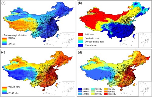
The remote sensing observations used in this study for $T_d$ retrieval come from MODIS, an instrument onboard the National Aeronautics and Space Administration’s (NASA’s) Earth Observing System (EOS) Terra and Aqua satellites. Both of these two satellites are in circular sun-synchronous orbits. The Terra overpass time is around 10:30 AM in its descending mode and 10:30 PM in its ascending mode, while the overpass time of Aqua is around 1:30 PM in its ascending mode and 1:30 AM in its descending mode. Four MODIS Version 6.1 products were adopted in this study, including MOD07_L2 and MOD11A1 provided by Terra MODIS as well as MYD07_L2 and MYD11A1 provided by Aqua MODIS. All these four products are largely limited to clear sky conditions. Considering the uncertainties caused by cloud contamination, this study only selected pixels flagged as the highest quality in MODIS cloud masking (Li et al. 2023; Zeng et al. 2018; Zhao and Duan 2020). MOD11A1 and MYD11A1 are daily land surface temperature & emissivity products with 1 km spatial resolution (Wan 2019). MOD07_L2 and MYD07_L2 are daily atmospheric profile products with 5 km spatial resolution (Borbas et al. 2015). These two products consist of several parameters, of which atmospheric moisture profile and surface air pressure were used in our work. Its atmospheric moisture profile is distributed at 20 vertical atmospheric pressure levels, which are 1000, 950, 920, 850, 780, 700, 620, 500, 400, 300, 250, 200, 150, 100, 70, 50, 30, 20, 10, and 5 hPa, respectively.

In addition to meteorological observations and MODIS products, the global aridity index (AI) dataset provided by the Consultative Group for International Agricultural Research-Consortium for Spatial Information (CGIAR-CSI) was used in this study. It defines AI as the ratio between mean annual precipitation and mean annual potential evapotranspiration. To be specific, this AI dataset with a spatial resolution of 30 arc seconds (∼ 1 km at the equator) is developed based on global raster climate datasets. These global climate datasets are available from WorldClim Global Climate Data (http://WorldClim.org), and the methods used for the derivation of AI are described in Zomer et al. (2007; 2008). Following United Nations Environment Programme (UNEP 1997), mainland China was divided into four climate zones in this study on the basis of AI values: arid (AI < 0.2), semi-arid (0.2 < AI < 0.5), dry sub-humid (0.5 < AI < 0.65) and humid (AI > 0.65) zone (Figure 1(b)).

3. Methodology

The ultimate objective of this study is to improve the accuracy of MODIS atmospheric profile products for the estimation of near-surface $T_d$. Four sections were designed as below to elaborate our methodology. Firstly, instantaneous $T_d$ at the daytime overpass time of Aqua and Terra satellites was retrieved from MODIS atmospheric profile products using two traditional methods so that a validation could be performed to evaluate the original accuracy of MOD07_L2 and MYD07_L2 products. The correction method proposed by Qiu et al. (2021) was designed to estimate daily mean $T_d$ from ground-based meteorological observations. Therefore, in the second section we estimated daily mean $T_d$ from a combination of MODIS land surface products and meteorological observations to test if this ground-based approach is suitable for large-scale remote sensing application. On the basis of the above two sections, this method was further modified in the third section to retrieve instantaneous $T_d$ through the combination of MODIS atmospheric profile and land surface products. Special attention was paid to investigate whether this modified approach could improve the original accuracy of MOD07_L2 and MYD07_L2 products and could be performed independently from ground observations. The fourth section describes the statistical metrics we used for accuracy evaluation.

3.1. Instantaneous ${\mathit{T}}_{\mathit{d}}$ retrieval from MODIS atmospheric profile products

As we reviewed in the introduction, according to the vertical levels used in previous studies, two approaches may be distinguished for the retrieval of near-surface $T_d$ from MODIS atmospheric profile products. Since MOD07_L2 and MYD07_L2 provide moisture profiles at 20 vertical pressure levels, the first approach extracts $T_d$ at the lowest vertical pressure (LVP) level as the surrogate for near-surface $T_d$ directly (Bisht et al. 2005; Byun, Liaqat, and Choi 2014; Venturini, Rodriguez, and Bisht 2011). The mathematical formula of this LVP method is expressed as: (3) $T_{d,int}^{LVP}=T_d^L$(3) where $T_{d,int}^{LVP}$ (${}^{\circ }\mathrm{C}$) represents near-surface $T_d$ estimates of the LVP method, the subscript ‘int’ denotes that this instantaneous $T_d$ was retrieved at the satellite overpass time, and $T_d^L$ (${}^{\circ }\mathrm{C}$) represents $T_d$ at the lowest vertical pressure level of MOD07_L2 and MYD07_L2 products. It should be noted that the lowest vertical pressure level is dependent on surface pressure, which varies with time and space. As a result, mainland China with a wide range of elevation, has a heterogeneous distribution of the lowest vertical pressure level. For illustration, the annual average surface pressure retrieved from MOD07_L2 is presented in Figure 1(c) to show the lowest vertical pressure level we used. To be specific, mainland China had an annual average surface pressure ranging from 476.42 to 1019.78 hPa. Controlled by the elevation patterns in Figure 1(a), a clear boundary (black line) was observed in its spatial distribution. The surface pressure was much higher in the southeast part. Another obvious characteristic is that Qinghai-Tibet Plateau had the lowest surface pressure. Accordingly, nine pressure levels were adopted as the lowest vertical pressure level in Eq. (3(3) $T_{d,int}^{LVP}=T_d^L$(3) ), which were 1000, 950, 920, 850, 780, 700, 620, 500, and 400 hPa, respectively (Figure 1(d)).

Considering the difference between surface pressure ($P^S$) and the available lowest pressure level ($P^L$), the second approach takes the hydrostatic assumption into account and interpolates $T_d$ at the two lowest pressure levels to near-surface level. Unlike the hypsometric equation (HE) used in Famiglietti et al. (2018), the adiabatic lapse rate (ALR) method proposed by Bisht and Bras (2010) and Zhu et al. (2017b) was adopted in this study to demonstrate the second approach as: (4) $ALR={\displaystyle \frac{T_d^L-T_d^U}{\mathrm{△}H}=\rho g{\displaystyle \frac{T_d^L-T_d^U}{P^L-P^U}}}$(4) (5) $T_{d,int}^{ALR}=T_d^L+{\displaystyle \frac{ALR}{\rho g}\left(P^S-P^L\right)=T_d^L+{\displaystyle \frac{T_d^L-T_d^U}{P^L-P^U}\left(P^S-P^L\right)}}$(5) where $T_{d,int}^{ALR}$ (${}^{\circ }\mathrm{C}$) represents near-surface $T_d$ estimates of the ALR method, $T_d^U$ (${}^{\circ }\mathrm{C}$) and $P^U$ (hPa) are the dew point temperature and atmospheric pressure retrieved at the upper pressure level of $P^L$, $\mathrm{△}H$ (m) is the height difference of these two pressure levels, $\rho$ ($kg/m^3$) is the density of the air, and $g$ ($m/s^2$) is the acceleration of gravity. The essence of HE and ARL methods is basically the same. Both of them interpolate moisture profile of MOD07_L2 and MYD07_L2 products into near-surface level by utilizing the two nearest pressure levels. The validity of HE method has already been evaluated by Famiglietti et al. (2018) on a global scale. That partly explains why this method was not adopted in our work. More importantly, both Famiglietti et al. (2018) and Zhang et al. (2021) suggest that the HE method would produce obvious outliers. Further statistical analysis is required to remove these outliers, which would eliminate 7.2% of all observations (Famiglietti et al. 2018).

3.2. Daily mean ${\mathit{T}}_{\mathit{d}}$ retrieval from MODIS and meteorological observations

The estimation of daily mean $T_d$ from daily minimum air temperature ($T_{amin}$) has been investigated in numerous studies based on in-situ meteorological observations (Dong et al. 2022; Mahmood and Hubbard 2005; Paredes et al. 2020; Todorovic, Karic, and Pereira 2013). Meanwhile, plenty of studies suggest that $T_{amin}$ estimates with high accuracy can be achieved by adopting MODIS nighttime land surface temperature ($T_s$) as proxy (Lin et al. 2012; Oyler et al. 2016; Vancutsem et al. 2010; Yoo et al. 2018; Zhu, Lű, and Jia 2013). The combination of these two aspects implies that MODIS land surface products have potential for the retrieval of near-surface $T_d$. As we mentioned in the introduction, due to the influence of climate conditions on the accuracy of $T_{amin}$-based $T_d$ estimation, a variety of correction methods have been proposed to lower this influence. Based on the correlation function between a dynamic factor (${\alpha }_T$) and aridity index (AI), Qiu et al. (2021) have recently developed a correction method regardless of climate zones. Their results show that this new method is superior to other correction methods in accuracy. Therefore, we adopted this method in our work to estimate near-surface $T_d$ from MODIS $T_s$ products.

The original method in Qiu et al. (2021) was developed to estimate daily mean $T_d$ using observations from 806 meteorological stations in mainland China. In order to perform a more robust validation and also lay a foundation for subsequent comparative analysis, we applied this method to 2153 meteorological stations across mainland China in this study. Specifically, this method was designed to estimate daily mean $T_d$ from $T_{amin}$ with a dynamic ${\alpha }_T$ (°C) regardless of climate zones as: (6) $e_{a,mean}=e_s\left(T_{d,mean}\right)\approx 0.6108\ast exp\left[{\displaystyle \frac{17.27\ast \left(T_{amin}-{\alpha }_T\right)}{\left(T_{amin}-{\alpha }_T\right)+237.3}}\right]$(6) (7) ${\alpha }_T=aln\left(AI\right)+b$(7) (8) $T_{d,mean}=T_{amin}-{\alpha }_T$(8) where $e_{a,mean}$ and $T_{d,mean}$ are the observed daily mean values of $e_a$ and $T_d$, and a and b are the fitted coefficients. Compared with the studies that assume near-surface $T_d$ to be equivalent to $T_{amin}$, ${\alpha }_T$ was added by Qiu et al. (2021) in the above equation for correction purpose. To be specific, ${\alpha }_T$ at site scale was determined by establishing its correlation function with AI based on a three-step procedure as below. Firstly, the annual average AI for each meteorological station was retrieved from the CGIAR-CSI AI dataset. Secondly, the ${\alpha }_T$ value of each meteorological station was determined with a non-linear regression method on the basis of Eq. (6(6) $e_{a,mean}=e_s\left(T_{d,mean}\right)\approx 0.6108\ast exp\left[{\displaystyle \frac{17.27\ast \left(T_{amin}-{\alpha }_T\right)}{\left(T_{amin}-{\alpha }_T\right)+237.3}}\right]$(6) ) using $e_{a,mean}$ and $T_{amin}$ observations of the year 2016. Thirdly, the correlation function between ${\alpha }_T$ and AI was calibrated across all sites using the logarithmic regression model presented in Eq. (7(7) ${\alpha }_T=aln\left(AI\right)+b$(7) ), and then applied to $T_{d,mean}$ estimation of the year 2017 for validation based on Eq. (8(8) $T_{d,mean}=T_{amin}-{\alpha }_T$(8) ). Qiu et al. (2021) have confirmed the validity of the above method at site scale using observations from 806 meteorological stations in mainland China. The focus of our work is to further investigate whether the observed $T_{amin}$ in Eq. (6(6) $e_{a,mean}=e_s\left(T_{d,mean}\right)\approx 0.6108\ast exp\left[{\displaystyle \frac{17.27\ast \left(T_{amin}-{\alpha }_T\right)}{\left(T_{amin}-{\alpha }_T\right)+237.3}}\right]$(6) ) could be replaced by MODIS nighttime $T_s$ so that $T_{d,mean}$ could be retrieved from MODIS land surface products in a spatially continuous manner. Accordingly, the estimation of $T_{d,mean}$ from MODIS land surface products was also performed following the above three steps. The only difference is that $T_{amin}$ used for calibration and validation was retrieved from MODIS nighttime $T_s$ rather than ground-based $T_{amin}$ observations. Considering the difference in overpass time between Terra and Aqua satellites, we applied this method to both MOD11A1 and MYD11A1 to conduct a comprehensive assessment.

3.3. An improved method for instantaneous ${\mathit{T}}_{\mathit{d}}$ retrieval from MODIS products

After knowing the original accuracy of MODIS atmospheric profile products for $T_{d,int}$ retrieval and Qiu et al. (2021)’s method for $T_{d,mean}$ retrieval, our attention was shifted to investigate whether Qiu et al. (2021)’s method can be modified to improve the accuracy of $T_{d,int}$ retrieval. Accordingly, Eq. (6(6) $e_{a,mean}=e_s\left(T_{d,mean}\right)\approx 0.6108\ast exp\left[{\displaystyle \frac{17.27\ast \left(T_{amin}-{\alpha }_T\right)}{\left(T_{amin}-{\alpha }_T\right)+237.3}}\right]$(6) ) and (8) were modified as below: (9) $e_{a,int}=e_s\left(T_{d,int}\right)\approx 0.6108\ast exp\left[{\displaystyle \frac{17.27\ast \left(T_{amin}-{\alpha }_T\right)}{\left(T_{amin}-{\alpha }_T\right)+237.3}}\right]$(9) (8) $T_{d,int}=T_{amin}-{\alpha }_T$(8)

The correlation function between ${\alpha }_T$ and AI was also established following the three steps in section 3.2. However, depending on the inputs used for the retrieval of ${\alpha }_T$ in Eq. (9(9) $e_{a,int}=e_s\left(T_{d,int}\right)\approx 0.6108\ast exp\left[{\displaystyle \frac{17.27\ast \left(T_{amin}-{\alpha }_T\right)}{\left(T_{amin}-{\alpha }_T\right)+237.3}}\right]$(9) ), three models can be identified. In the first model, both $T_{d,int}$ and $T_{amin}$ were retrieved from meteorological observations to evaluate the performance of this correction method at site scale. In order to coincide with $T_{d,int}$ retrieved from MODIS atmospheric profile products, $T_{d,hour}$ observed at the time that most approximates satellite overpass time was used as the proxy for $T_{d,int}$. It means that the time interval between meteorological and satellite observations was less than 30 min. In the second model, ground-based $T_{amin}$ observations of the first model were replaced by MODIS nighttime $T_s$ so that $T_{d,int}$ could be retrieved from MODIS land surface products in a spatially continuous manner. 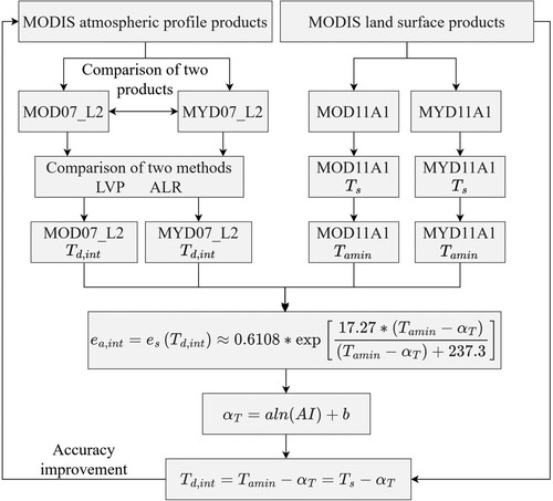Thirdly, ground $T_{d,int}$ observations of the second model were further substituted by $T_{d,int}^{LVP}$ and $T_{d,int}^{ALR}$ to investigate whether this correction method can improve the original accuracy of MODIS atmospheric profile products independently from ground observations. Figure 2 shows the flowchart of the above $T_{d,int}$ estimation.

Figure 2. Flowchart of the methods we adopted for $T_{d,int}$ estimation.

3.4. Statistical metrics

Following Famiglietti et al. (2018), we adopted three statistical metrics in this study for accuracy evaluation, including the coefficient of determination (R²), root mean square error (RMSE), and bias (B). With the in-situ observations as input, R² was determined by fitting a regression line through the origin. The equations of RMSE and B are expressed as: (11) $\begin{array}{c}RMSE=\sqrt{{\displaystyle \frac{1}{n}\sum _{i=1}^n{\left(x_i-y_i\right)}^2}}\end{array}$(11) (12) $\begin{array}{c}B={\overline{x}}_i-{\overline{y}}_i\end{array}$(12) where $n$ represents the total sample size; subscript $i$ represents the sample number at the $i^{th}$ position;$x_i$ and $y_i$ represent the estimated and observed near-surface $T_d$; and ${\overline{x}}_i$ and ${\overline{y}}_i$ represent the mean values of $T_d$ estimation and observation, respectively. It should be noted that the calibration of ${\alpha }_T$ for each meteorological station was performed using $T_d$ and $T_{amin}$ observations of the year 2016. The evaluation of its validity was conducted using $T_d$ observations of the year 2017.

4. Results

4.1. Original accuracy of MODIS atmospheric profile products

Table 1 shows the original accuracy of MOD07_L2 and MYD07_L2 products for the representation of instantaneous dew point temperature ($T_{d,int}$). For MOD07_L2, the ALR method was superior to LVP method in all statistical metrics. The R², RMSE and B of $T_{d,int}^{ALR}$ in two full years were 0.84, 5.82 °C, and 0.88 °C, and those of $T_{d,int}^{LVP}$ estimates were 0.81, 6.50 °C, and −1.24 °C, respectively. The statistics of the individual year 2016 and 2017 have also confirmed the superiority of ALR method. However, when the same comparison was performed for MYD07_L2 product, the opposite situation was observed. All statistical metrics indicate that the LVP method provided a better $T_{d,int}$ retrieval. The R², RMSE and B it achieved in two full years were 0.75, 7.42 °C, and 0.91 °C, and those achieved by the ALR method were 0.74, 7.70 °C, and 2.63 °C, respectively. Judged from B values, the LVP method underestimated $T_{d,int}$ for MOD07_L2 while overestimated $T_{d,int}$ for MYD07_L2. In contrast, the ALR method overestimated $T_{d,int}$ for both products. In general, MOD07_L2 was a better proxy for near-surface $T_d$, because it provided $T_{d,int}$ estimation with higher accuracy in either of these two methods. Even the accuracy achieved by the better method for MYD07_L2 was still lower than that produced by the worse method for MOD07_L2. The reasons behind can be explained by the satellite overpass time. The overpass time of Terra and Aqua is around 10:30 AM and 1:30 PM, respectively. It is obvious that the solar radiation at the Aqua overpass time is much stronger. Consequently, the complex interaction of the surface energy balance system makes the retrieval of $T_d$ from MYD07_L2 far from straightforward.

Table 1. Accuracy of MODIS atmospheric profile products for $T_{d,int}$ estimation.

Product	Method	Year	n	R^2	RMSE (°C)	B (°C)
MOD07_L2	LVP	2016	247454	0.83	6.48	−1.57
		2017	243691	0.80	6.52	−0.90
		2016–2017	491145	0.81	6.50	−1.24
	ALR	2016	247454	0.85	5.70	0.59
		2017	243691	0.83	5.94	1.18
		2016–2017	491145	0.84	5.82	0.88
MYD07_L2	LVP	2016	272995	0.77	7.20	0.61
		2017	261234	0.72	7.65	1.23
		2016–2017	534229	0.75	7.42	0.91
	ALR	2016	272995	0.77	7.45	2.36
		2017	261234	0.72	7.95	2.91
		2016–2017	534229	0.74	7.70	2.63

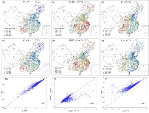
In order to investigate the spatial patterns of $T_{d,int}$ accuracy, Figure 3 presents the distribution of these three statistical metrics at site scale as well as their scatterplots achieved by different methods. Considering the significant advantage of MOD07_L2 over MYD07_L2, here we only adopted MOD07_L2 product to investigate the difference between LVP and ALR methods. In general, these methods have achieved similar patterns in the spatial distribution of these three metrics. Their correlation of R², RMSE and B across 2153 stations was 0.97, 0.69, and 0.81, respectively. Both methods generated $T_{d,int}$ estimates correlated better with observations in the east of the mainland, which coincided well with the three major plains in China. Similarly, stations with relatively low R² values were mainly concentrated in Yunnan province. The RMSE of $T_{d,int}^{LVP}$ and $T_{d,int}^{ALR}$ ranged from 3.23 to 20.25 °C and from 2.65 to 14.46 °C, respectively. This confirms the superiority of ALR over LVP method from another perspective. The scatterplots of B reveal the key difference between these two methods. The B achieved by the ALR was always larger than that achieved by the LVP. It means that a positive adiabatic lapse rate was retrieved from MODIS atmospheric profile products in Eq. (4(4) $ALR={\displaystyle \frac{T_d^L-T_d^U}{\mathrm{△}H}=\rho g{\displaystyle \frac{T_d^L-T_d^U}{P^L-P^U}}}$(4) ). Consequently, the interpolation from the lowest pressure level to near-surface level would increase $T_{d,int}$ from $T_{d,int}^{LVP}$ to $T_{d,int}^{ALR}$. That also explains why $T_{d,int}^{ALR}$ had a much smaller number of stations with negative B values than $T_{d,int}^{LVP}$. To be specific, the LVP method underestimated $T_{d,int}$ for 56.64% of the 2153 stations, which were widely distributed in Midwest China, Hainan province, Anhui province, Fujian province, and parts of Northeast China. In comparison, although the stations with negative B values produced by the ALR method were also located in the above regions, their number only accounted for 34.09% of the 2153 stations. Considering the altitude is obviously higher in Midwest China, the above results imply that the accuracy of MODIS atmospheric profile products is closely related to topography (Mendez 2004).

Figure 3. Accuracy of $T_{d,int}$ retrieved from MOD07_L2 product at site scale and their scatterplots. (a) – (c) are R², RMSE and B achieved by the LVP method, (d) – (f) are R², RMSE and B achieved by the ALR method, and (g) – (i) are the scatterplots of R², RMSE and B achieved by these two methods.

4.2. Accuracy of the new method for daily mean dew point temperature estimation

Based on ${\alpha }_T$ retrieved from Eq. (6(6) $e_{a,mean}=e_s\left(T_{d,mean}\right)\approx 0.6108\ast exp\left[{\displaystyle \frac{17.27\ast \left(T_{amin}-{\alpha }_T\right)}{\left(T_{amin}-{\alpha }_T\right)+237.3}}\right]$(6) ), the relationship between ${\alpha }_T$ and AI across 2153 stations of the year 2016 was established using the logarithmic regression model of Eq. (7(7) ${\alpha }_T=aln\left(AI\right)+b$(7) ). The results are presented in Figure 4. For MOD11A1 product, the a and b calibrated by $T_{d,mean}$ and $T_{amin}$ observations were −2.01 and 1.39 with $R^2$ of 0.47 (Figure 4(a)), and the a and b calibrated by $T_{d,mean}$ observations and MOD11A1 nighttime $T_s$ were −1.97 and 2.31 with $R^2$ of 0.46 (Figure 4(b)). As for MYD11A1, the a and b calibrated by $T_{d,mean}$ and $T_{amin}$ observations were −1.98 and 1.32 with $R^2$ of 0.45 (Figure 4(c)), and the a and b calibrated by $T_{d,mean}$ observations and MYD11A1 nighttime $T_s$ were −1.65 and 0.98 with $R^2$ of 0.36 (Figure 4(d)). It should be noted that both Figure 4(a,c) were retrieved from ground-based $T_{d,mean}$ and $T_{amin}$ observations. The difference in their coefficients was completely caused by the difference in samples. In contrast, the difference in coefficients between Figure 4(b,d) was mainly caused by the difference between MOD11A1 and MYD11A1 for the representation of $T_{amin}$. Applying the above models to the year 2017, we validated and presented their accuracy in Figure 5. The accuracy of $T_{amin}$ as a direct surrogate for $T_{d,mean}$ is also presented for comparison. As expected, $T_{amin}$ as a direct proxy for $T_{d,mean}$ would lead to significant overestimation, with B and RMSE as high as 3.41∼3.47 °C and 5.59∼5.63 °C, respectively. This confirms the necessity of correction methods for the accurate $T_d$ estimation from $T_{amin}$. To be specific, the ground-based correction method proposed by Qiu et al. (2021) has improved the accuracy significantly, with B and RMSE around 0.59∼0.60 °C and 4.18∼4.19 °C, respectively. In comparison, the B and RMSE achieved by MOD11A1-based correction method were 0.69 and 4.62 °C, and those achieved by MYD11A1 product were 0.63 and 4.42 °C, respectively. Both two statistics indicate that MODIS land surface products as proxy for $T_{amin}$ would reduce the accuracy of the above correction method slightly.

Figure 4. Logarithmic regression models between ${\alpha }_T$ and AI for $T_{d,mean}$ estimation. (a) and (c) represent models calibrated by $T_{d,mean}$ and $T_{amin}$ observations, (b) represents model calibrated by $T_{d,mean}$ observations and MOD11A1 nighttime $T_s$, and (d) represents model calibrated by $T_{d,mean}$ observations and MYD11A1 nighttime $T_s$.

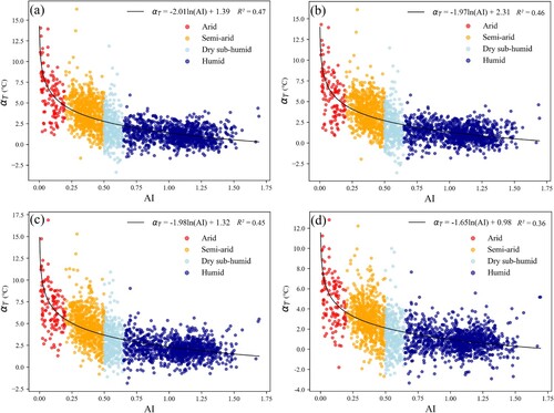
Figure 5. Accuracy of $T_{d,mean}$ estimation achieved by different methods. (a) and (d) are the accuracy of $T_{amin}$ as a direct proxy for $T_{d,mean}$, (b) and (e) are the accuracy of the correction method calibrated by $T_{amin}$ observations, and (c) and (f) are the accuracy of the correction method calibrated by MOD11A1 and MYD11A1 $T_s$, respectively.

The above correction method was developed on the basis of AI. Therefore, it is necessary to investigate its performance in different climate zones. The results are presented in Table 2. For simplicity, the $T_{d,mean}$ estimated directly by $T_{amin}$, by the correction method developed from $T_{d,mean}$ and $T_{amin}$ observations, and by the correction method developed from $T_{d,mean}$ observations and MODIS $T_s$ was renamed as method Ⅰ, Ⅱ, and Ⅲ, respectively. Both R² and RMSE show that the accuracy of these methods increased gradually from arid to humid regions. It implies that these $T_{amin}$-based methods are more suitable for $T_d$ estimation in humid regions. Judged from B values, the accuracy of method Ⅰ still increased gradually from arid to humid regions. However, this finding did not hold true for the ${\alpha }_T$-based correction methods. As for the accuracy difference of these three methods, two ${\alpha }_T$-based correction methods were always superior to method Ⅰ in terms of B values. However, in terms of RMSE, although these two ${\alpha }_T$-based correction methods were still superior in most regions, their superiority seemed to decrease gradually from arid to humid zones. This is particularly obvious for method Ⅲ. Take MOD11A1 as an example. In arid, semi-arid, and dry sub-humid zones, the RMSE of method Ⅰ was reduced by method Ⅲ from 8.46 to 5.91 °C, from 6.72 to 5.05 °C, and from 4.76 to 4.48 °C, respectively. It is obvious that the decrease rate became lower and lower. In humid zone, method Ⅰ was even superior to method Ⅲ in terms of RMSE. The advantage of method Ⅱ over method Ⅰ also decreased gradually from arid to humid zones, but the RMSE it produced was always lower than that produced by method Ⅰ. Therefore, the poor performance of method Ⅲ in humid region was mainly caused by the errors involved in the retrieval of $T_{amin}$ from MODIS land surface products.

Table 2. Accuracy of daily mean dew pint temperature estimates achieved by different methods. The unit of RMSE and B is °C.

Product	Method	Metrics	All n = 2153	Arid n = 122	Semi-arid n = 684	Dry sub-humid n = 301	Humid n = 1046
MOD11A1	I	R²	0.88	0.80	0.87	0.91	0.94
		RMSE	5.63	8.46	6.72	4.76	3.07
		B	3.47	6.32	4.76	2.63	1.56
	II	R²	0.90	0.80	0.87	0.91	0.94
		RMSE	4.18	5.53	4.88	3.96	2.68
		B	0.59	−0.14	1.28	0.07	0.17
	III	R²	0.88	0.79	0.86	0.88	0.88
		RMSE	4.62	5.91	5.05	4.48	3.66
		B	0.69	0.01	1.33	0.28	0.27
MYD11A1	I	R²	0.88	0.80	0.87	0.91	0.94
		RMSE	5.59	8.40	6.62	4.70	3.06
		B	3.41	6.26	4.63	2.50	1.54
	II	R²	0.90	0.80	0.87	0.91	0.94
		RMSE	4.19	5.50	4.86	3.97	2.68
		B	0.60	−0.07	1.25	0.03	0.21
	III	R²	0.90	0.81	0.87	0.89	0.89
		RMSE	4.42	5.39	4.77	4.38	3.62
		B	0.63	0.15	1.16	0.06	0.34

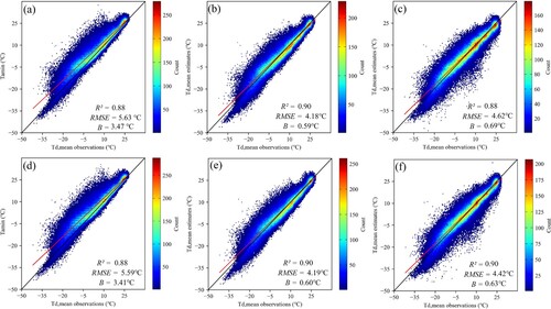
4.3. Accuracy of the method for instantaneous dew point temperature estimation

The above analysis indicates that the correction method calibrated by MODIS $T_s$ has achieved similar accuracy with that calibrated by ground $T_{amin}$ observations for $T_{d,mean}$ estimation. This lays a good basis for its application in instantaneous $T_d$ estimation. Figure 6 shows the logarithmic regression models we calibrated for $T_{d,int}$ estimation based on the pooled data of the year 2016. Four models should be distinguished here: the model retrieved from ground-based $T_{d,int}$ and $T_{amin}$ observations (Figure 6(a,e)), the model retrieved from ground-based $T_{d,int}$ observations and MODIS $T_s$ (Figure 6(b,f)), the model retrieved from MODIS $T_{d,int}^{LVP}$ and $T_s$ (Figure 6(c,g)), and the model retrieved from MODIS $T_{d,int}^{ALR}$ and $T_s$ (Figure 6(d,h)). The first two models need meteorological observations for calibration. In contrast, the remaining two models were totally established based on MODIS products. Table 3 shows the accuracy of these models in the year 2017. The original accuracy of $T_{d,int}^{LVP}$ and $T_{d,int}^{ALR}$ is also presented for comparison. In general, similar accuracy has been achieved by these four models. The R² they produced was almost the same with each other. The RMSE achieved by Terra and Aqua MODIS ranged from 5.22 to 5.33 °C and from 5.47 to 6.21 °C, respectively. Although higher accuracy was still achieved by the first two ground-based models, their RMSE was only a little lower than that produced by the two models independently from ground observations. This is particularly obvious for Terra MODIS, the largest RMSE difference of which was only 0.11 °C. Compared with the original $T_{d,int}^{LVP}$ and $T_{d,int}^{ALR}$, all metrics show that these four models have improved their accuracy significantly. Take the two models that were totally developed from MODIS products as an example. The RMSE of $T_{d,int}^{LVP}$ and $T_{d,int}^{ALR}$ for Terra MODIS has been reduced from 6.89 to 5.23 °C and from 6.20 to 5.33 °C, respectively. For Aqua MODIS, its RMSE has been reduced from 8.07 to 5.59 °C and from 8.35 to 6.21 °C, respectively. Obviously, the accuracy of MODIS atmospheric profile products can be improved significantly through the introduction of MODIS land surface products.

Figure 6. Logarithmic regression models between ${\alpha }_T$ and AI for $T_{d,int}$ estimation. (a) - (d) are models for $T_{d,int}$ estimation at Terra overpass time, and (e) - (h) are models for $T_{d,int}$ estimation at Aqua overpass time.

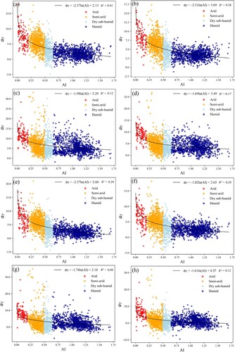
Table 3. Accuracy of instantaneous dew pint temperature estimates achieved by different methods. For simplicity, the $T_{d,int}$ estimated from $T_{d,int}$ and $T_{amin}$ observations, from $T_{d,int}$ observations and $T_s$, from $T_{d,int}^{LVP}$ and $T_s$, and from $T_{d,int}^{ALR}$ and $T_s$ was renamed as$T_{d,int}-T_{amin}$, $T_{d,int}-T_s$, $T_{d,int}^{LVP}-T_s$, and$T_{d,int}^{ALR}-T_s$, respectively. The unit of RMSE and B is °C.

Product	Metrics	$T_{d,int}^{LVP}$	$T_{d,int}^{ALR}$	$T_{d,int}-T_{amin}$	$T_{d,int}-T_s$	$T_{d,int}^{LVP}-T_s$	$T_{d,int}^{ALR}-T_s$
Terra MODIS	n	104260	104260	104260	104260	104260	104260
	R^2	0.77	0.81	0.86	0.87	0.87	0.87
	RMSE	6.89	6.20	5.22	5.22	5.23	5.33
	B	−0.84	1.37	0.62	0.70	−0.79	1.24
Aqua MODIS	n	110609	110609	110609	110609	110609	110609
	R^2	0.69	0.70	0.86	0.87	0.87	0.87
	RMSE	8.07	8.35	5.47	5.47	5.59	6.21
	B	1.46	3.28	0.79	0.82	1.43	3.07

The accuracy in Table 3 was achieved by applying the models calibrated in 2016 to the year 2017. This is necessary for the validation of the first two ground-based models. However, the remaining two models were totally established from MODIS products, which means that they are calibration-independent. Accordingly, Table 4 shows the accuracy of these two models established from MODIS products of the year 2017. In view of the significant superiority of Terra MODIS over Aqua MODIS in Table 3, we only focused on Terra MODIS products here for further analysis. Across all stations the R², RMSE, and B achieved by the $T_{d,int}^{LVP}$-based correction method were 0.85, 5.22 °C, and −0.65 °C, and those achieved by the $T_{d,int}^{ALR}$-based correction method were 0.85, 5.35 °C, and 1.36 °C, respectively. All these statistics were very close to those in Table 3, which demonstrates the portability of these correction methods in different years. Both R² and RMSE suggest that the accuracy of these ${\alpha }_T$-based correction methods increased gradually from arid to humid regions, which is consistent with the findings in Table 2. The R² produced by these two correction methods was the same with each other in all climate zones. However, the RMSE achieved by the $T_{d,int}^{ALR}$-based correction method was lower than that achieved by the $T_{d,int}^{LVP}$-based correction method in three out of the four climate zones. This basically follows the same order with the original accuracy of $T_{d,int}^{LVP}$ and $T_{d,int}^{ALR}$. It suggests that the accuracy of these correction methods is still controlled by the original accuracy of $T_{d,int}$ estimation. Compared with the original $T_{d,int}^{LVP}$ and $T_{d,int}^{ALR}$, both R² and RMSE indicate that these correction methods have distinct advantages in semi-arid, dry sub-humid, and humid zones. However, their RMSE in arid zone was much larger than that produced by the original $T_{d,int}^{LVP}$ and $T_{d,int}^{ALR}$. This confirms again that these correction methods are more suitable for $T_d$ estimation in humid regions.

Table 4. Accuracy of instantaneous dew pint temperature estimates achieved by different methods for the year 2017. $T_{d,int}^{LVP}-T_s$ and $T_{d,int}^{ALR}-T_s$ represent the correction method developed from $T_{d,int}^{LVP}$ and $T_s$ and from $T_{d,int}^{ALR}$ and $T_s$, respectively. The unit of RMSE and B is °C.

Method	Metrics	All n = 2153	Arid n = 122	Semi-arid n = 684	Dry sub-humid n = 301	Humid n = 1046
LVP	R²	0.74	0.74	0.72	0.74	0.70
	RMSE	6.89	6.27	7.27	7.27	6.25
	B	−0.84	−2.46	0.18	−1.61	−1.43
$T_{d,int}^{LVP}-T_s$	R²	0.85	0.74	0.83	0.85	0.87
	RMSE	5.22	6.91	5.53	5.14	4.02
	B	−0.65	−1.97	−0.01	−1.28	−0.86
ALR	R²	0.79	0.74	0.77	0.79	0.76
	RMSE	6.20	5.63	6.90	5.99	5.31
	B	1.37	−0.17	2.45	1.05	0.42
$T_{d,int}^{ALR}-T_s$	R²	0.85	0.74	0.83	0.85	0.87
	RMSE	5.35	6.63	5.91	5.02	4.01
	B	1.36	0.63	2.09	0.66	0.89

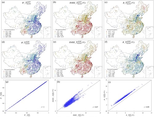
Figure 7 presents the distribution of these three metrics at site scale to investigate the spatial difference of these two correction methods. To be consistent with Figure 3, these metrics were also retrieved from $T_{d,int}$ estimations in two full years. Both two methods were developed from MOD11A1 nighttime $T_s$ in a form of $T_{d,int}=T_s-{\alpha }_T$. The only difference is that their ${\alpha }_T$ was retrieved from $T_{d,int}^{LVP}$ and $T_{d,int}^{ALR}$ respectively. As a result, the R² they produced was the same with each other, which ranged from 0.21 to 0.96 with a median of 0.86. Compared with Figure 3, the correction methods have improved the R² values for most stations, which is particularly obvious in the middle and lower reaches of the Yangtze River, South China, and East China. These correction methods also demonstrated significant advantage in terms of RMSE. The RMSE of $T_{d,int}^{LVP}$-based correction method ranged from 1.97 to 12.19 °C with a median of 4.57 °C, and that achieved by $T_{d,int}^{ALR}$-based correction method ranged from 1.50 to 13.69 °C with a median of 4.40 °C. In comparison, the median of RMSE produced by the original $T_{d,int}^{LVP}$ and $T_{d,int}^{ALR}$ was 5.50 and 5.22 °C, respectively. The B values achieved by these two correction methods correlated well with each other with r as high as 0.99. However, the $T_{d,int}^{ALR}$-based correction method always produced B values larger than $T_{d,int}^{LVP}$-based correction method. This followed the same order with the original B of $T_{d,int}^{LVP}$ and $T_{d,int}^{ALR}$. Compared with Figure 3, the $T_{d,int}^{LVP}$-based correction method has reduced the number of stations with serious underestimation significantly, which is particularly obvious in the southwest of China. As for the $T_{d,int}^{ALR}$-based correction method, it has not only reduced the number of stations with serious underestimation in the southwest of China, but also reduced the number of stations with obvious overestimation in Qinghai, Guangdong, Guangxi, and Liaoning province significantly.

Figure 7. Accuracy of $T_{d,int}$ estimates achieved by correction methods at site scale and their scatterplots. (a) – (c) are R², RMSE and B achieved by the $T_{d,int}^{LVP}$-based correction method, (d) – (f) are R², RMSE and B achieved by the $T_{d,int}^{ALR}$-based correction method, and (g) – (i) are the scatterplots of R², RMSE and B achieved by these two methods.

5. Discussion

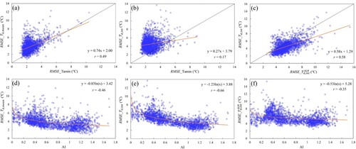
Implicitly or explicitly, the analysis in the above section has pointed out that the performance of Qiu et al. (2021)’s correction method is influenced by several factors in large-scale remote sensing application. We would go through these factors and the uncertainties involved in this section.

Firstly, MODIS nighttime $T_s$ was adopted in this study as the proxy for $T_{amin}$ so that the ground-based correction method can be performed over large scale based on MODIS products. The validity of this substitution is assessed in Figure 8. As expected, MYD11A1 was a better proxy for $T_{amin}$. Its R², RMSE, and B across all stations were 0.96, 2.78 °C, and −0.61 °C, and those achieved by MOD11A1 were 0.95, 3.00 °C, and 0.94 °C, respectively. That explains why the correction method developed from MYD11A1 performed a little better than that developed from MOD11A1 for $T_{d,mean}$ estimation (Figure 5). The overpass time of Terra and Aqua during the night is 10:30 pm and 1:30 am, respectively. Aqua has overpass time much closer to that the daily minimum air temperature occurs. That might be the reason why MYD11A1 was a better proxy for $T_{amin}$ (Vancutsem et al. 2010; Zhu, Lű, and Jia 2013). Figure 9(a) shows the scatterplots of the RMSE achieved by MYD11A1 for $T_{amin}$ estimation versus the RMSE achieved by correction method for $T_{d,mean}$ estimation. Their RMSE correlated well with each other with r as 0.49. An increase of 1 °C in the RMSE of $T_{amin}$ estimation would lead to an increase of 0.74 °C in the RMSE of $T_{d,mean}$ estimation on average. As for the correction method for $T_{d,int}$ estimation, the r between its RMSE and that achieved by MOD11A1 for $T_{amin}$ estimation was only 0.17 (Figure 9(b)). In contrast, its RMSE correlated significantly with the original RMSE of $T_{d,int}^{ALR}$ retrieval with r as high as 0.58 (Figure 9(c)). Due to the effect of correction method, an increase of 1 °C in the original RMSE of $T_{d,int}^{ALR}$ would only lead to an increase of 0.58 °C in the RMSE of final $T_{d,int}$ estimation on average. Therefore, compared with the accuracy of MODIS nighttime $T_s$ as the proxy for $T_{amin}$, the original accuracy of MODIS atmospheric profile products had a much greater impact on the accuracy of our modified correction method for $T_{d,int}$ estimation. The comparison in Table 1 suggests that the $T_{d,int}$ retrieved from MOD07_L2 was superior to that retrieved from MYD07_L2 in accuracy. The combination of these findings explains why the correction method developed from MOD07_L2 was superior to that developed from MYD07_L2.

Figure 8. Accuracy of MOD11A1 (a) and MYD11A1 (b) nighttime $T_s$ as the proxy for $T_{amin}$.

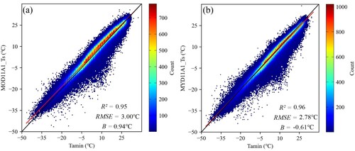
Figure 9. Relationships of the RMSE achieved by different estimates with each other and their variations with AI. (a) and (b) are the scatterplots of the RMSE achieved for $T_{d,mean}$ and $T_{d,int}$ estimation with the RMSE achieved for $T_{amin}$ estimation, respectively. (c) is the scatterplots of the RMSE achieved for $T_{d,int}$ estimation with the RMSE achieved by $T_{d,int}^{ALR}$. (d) – (f) are the variations of the RMSE achieved by $T_{d,mean}$, $T_{d,int}$ and $T_{d,int}^{ALR}$ estimation with AI, respectively.

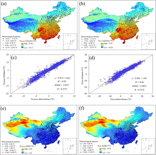
Besides the original accuracy of MODIS atmospheric profile and land surface products, AI was another main factor influencing the performance of these correction methods. Its impact at site scale has already been presented in Tables 2 and 4. Compared with the original method proposed by Qiu et al. (2021), the main contribution of our work is that their ground-based method was modified for large-scale remote sensing applications. Accordingly, $T_d$ could be estimated and mapped from MODIS products for whole mainland China. So here we further investigated the accuracy and uncertainties of these AI-based correction methods in a spatially continuous manner. Figure 10(a,b) show the spatial distribution of our annual average $T_{d,mean}$ and $T_{d,int}$ estimates, respectively. A close look at these two figures indicates that the estimated $T_{d,mean}$ and $T_{d,int}$ at pixel scale agreed very well with the ground-based observations at site scale. For illustration, Figure 10(c,d) show these comparisons across 2153 meteorological stations. It is obvious that these correction methods have achieved good performance in capturing the annual average $T_d$ patterns. The R², RMSE, and B of annual average $T_{d,mean}$ estimates were 0.95, 1.84, and 0.53 °C, and those achieved for annual average $T_{d,int}$ estimates were 0.94, 2.09 °C, and 0.75 °C, respectively. The accuracy of $T_{d,int}$ estimates was still a little lower than that achieved for $T_{d,mean}$ estimates, but it must be noted that the estimation of $T_{d,int}$ was performed independently from ground-based observations. In order to investigate the uncertainties involved in our above $T_{d,mean}$ and $T_{d,int}$ estimates in a spatially continuous manner, we first present the variations of their RMSE with AI across all sites (Figure 9(d,e), respectively). The RMSE of the original $T_{d,int}^{ALR}$ versus AI is presented in Figure 9(f) for comparison. As expected, the RMSE of both $T_{d,mean}$ and $T_{d,int}$ estimation decreased generally with the increase of AI. What is unexpected is that the RMSE of the original $T_{d,int}^{ALR}$ was also negatively correlated with AI. It implies that not only the correction methods but also the original MODIS atmospheric profile product were more suitable for $T_d$ estimation in humid regions. On this basis, we present the RMSE of our $T_{d,mean}$ and $T_{d,int}$ estimates in Figure 10(e,f) by applying the logarithmic regression models established in Figure 9(d,e) to mainland China. Specifically, in arid, semi-arid, dry sub-humid, and humid zone, the average RMSE of $T_{d,mean}$ estimates were 5.87, 4.36, 3.89, and 3.42 °C, and the average RMSE of $T_{d,int}$ estimates were 7.41, 5.24, 4.56, and 3.88 °C, respectively. Both $T_{d,mean}$ and $T_{d,int}$ estimates indicate that this AI-based correction method was more suitable for $T_d$ estimation in humid climate.

Figure 10. Spatial distribution of annual average $T_d$ estimation and RMSE as well as their accuracy across all sites. (a) and (b) are the spatial distribution of annual average $T_{d,mean}$ and $T_{d,int}$ estimation, (c) and (d) are the accuracy of annual average $T_{d,mean}$ and $T_{d,int}$ estimation across all sites, and (e) and (f) are the spatial distribution of the average RMSE retrieved from the logarithmic regression models in Figure 9(d,e).

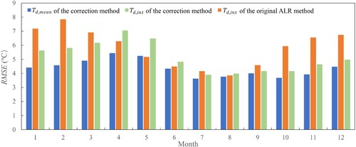
Influenced by the East Asian monsoon, both precipitation and temperature in China have obvious seasonal variations. It implies that the seasonal variability may have additionally affected the accuracy of $T_d$ estimation. Figure 11 shows the RMSE of $T_{d,mean}$ and $T_{d,int}$ estimates as well as the original $T_{d,int}^{ALR}$ in different months. As expected, the accuracy of these three estimates had significant seasonal variations. All of them achieved the lowest RMSE in warm and humid months such as July and August. This confirms again that both the correction method and the original MODIS atmospheric profile product are more suitable for $T_d$ estimation in humid climate. The correction method adopted in this study was developed from an annual average AI provided by the CGIAR-CSI. As a result, the correction factor (${\alpha }_T$) derived from AI was a constant without seasonal variations. The above analysis suggests that a temporal dynamic ${\alpha }_T$ retrieved from monthly climatic variables holds potential for the improvement of this correction method. As for the inter-comparison of these three estimates, the lowest RMSE was achieved by $T_{d,mean}$ estimates in all months except for May. It implies that the estimation of instantaneous $T_d$ was much more complex than the retrieval of its daily mean value. The accuracy of original $T_{d,int}^{ALR}$ estimates has been improved by the correction method in eight months including January, February, March, July, September, October, November, and December. The accuracy improvement in dry and cold months was much more significant than that observed in humid and warm months. The RMSE of $T_{d,int}^{ALR}$ estimates in April, May, June and August were even lower than that achieved by the correction method. This is consistent with the finding in Table 2 that the superiority of this correction method decreased gradually from arid to humid zones. All these results confirm the necessity of a temporal dynamic ${\alpha }_T$ for the further development of this correction method.

Figure 11. Seasonal variations of the RMSE achieved by the ALR and correction methods.

6. Conclusion

Near-surface $T_d$ serves as indispensable input in many hydrological, climatological, and ecological models. The need for $T_d$ with fine resolution results in numerous studies looking into MODIS atmospheric profile products for help. However, the accuracy of these products over large scale has seldom been evaluated, making the quality of their $T_d$ retrieval for many modeling applications relatively unknown. Given this background, a large-scale validation was performed in this study across mainland China, aiming to evaluate the accuracy of these products for $T_d$ retrieval comprehensively. On this basis, a recent ground-based correction method was modified to further improve their accuracy.

The accuracy of MODIS atmospheric profile products varied with $T_d$ retrieval methods. For MOD07_L2, the ALR method was superior to LVP method in all evaluation metrics. However, all metrics show that the LVP method provided a better $T_d$ retrieval for MYD07_L2. Nonetheless, MOD07_L2 was suggested in this study because it achieved higher accuracy in either of these two methods. The RMSE it achieved by LVP and ALR method was 6.50 and 5.82 °C, respectively. In comparison, the RMSE achieved by LVP and ALR method for MYD07_L2 was 7.42 and 7.70 °C, respectively. After knowing the original accuracy of MODIS atmospheric profile products, we adopted and modified a ground-based correction method to further improve their accuracy. The focus of our modification is to investigate whether this ground-based approach is applicable to large-scale remote sensing applications. To be specific, this ground-based method was developed based on the correlation function between a correction factor (${\alpha }_T$) and AI. ${\alpha }_T$ derived from AI was used to correct the estimation of $T_d$ from daily minimum air temperature ($T_{amin}$). In our modified approach, $T_{amin}$ was retrieved from MODIS nighttime land surface temperature rather than ground observation, so it is applicable to large-scale remote sensing applications. The results show that although the uncertainty increases generally with the decrease of AI, this modified method still holds great potential to improve the accuracy of $T_d$ estimates independently from ground observations. The RMSE achieved by LVP and ALR method for MOD07_L2 has been reduced to 5.23 and 5.33 °C, and the RMSE achieved by LVP and ALR method for MYD07_L2 has been reduced to 5.59 and 6.21 °C, respectively. It was particularly useful in capturing the annual average $T_d$ patterns. The R², RMSE, and bias of annual average daily mean $T_d$ estimates were 0.95, 1.84 °C, and 0.53 °C, and those achieved for annual average instantaneous $T_d$ estimates were 0.94, 2.09 °C, and 0.75 °C, respectively.

Despite the above advantages, our modified approach still suffers from drawbacks. Firstly, its performance was influenced significantly by the original accuracy of MODIS atmospheric profile products. It will benefit from the development of new $T_d$ retrieval methods from MODIS atmospheric profile products (Famiglietti et al. 2018). Secondly, the validity of this AI-based correction method was sensitive to AI values (Qiu et al. 2021; Raziei and Pereira 2013). Its accuracy increased generally from arid to humid regions. Similarly, significant seasonal variations were observed in its performance. These findings imply that a temporal dynamic ${\alpha }_T$ is necessary for the further development of this method.

Acknowledgements

We are highly grateful to the MODIS mission scientists and associated NASA personnel for their data support. We also acknowledge the providers of meteorological observations and global aridity index dataset, namely, the China Meteorological Data Service Center and the Consultative Group for International Agricultural Research-Consortium for Spatial Information. We also thank the anonymous reviewers for their comments and suggestions that improved this paper.

Disclosure statement

No potential conflict of interest was reported by the author(s).

Data availability statement

MODIS products were obtained from https://ladsweb.modaps.eosdis.nasa.gov/archive/allData/61, meteorological observations were obtained from the China Meteorological Data Service Center at http://data.cma.cn/en/?r=data/detail&dataCode=J.0019.0010.S002, and aridity index dataset was obtained from https://cgiarcsi.community/data/global-aridity-and-pet-database/.

Additional information

Funding

This work was supported by Ministry of Science and Technology of the People's Republic of China [grant number: 2021YFC3000201]; National Natural Science Foundation of China [grant number: 42071032]; Youth Innovation Promotion Association of the Chinese Academy of Sciences [grant number: 2020056].

References

- Ali, H., H. J. Fowler, and V. Mishra. 2018. “Global Observational Evidence of Strong Linkage Between Dew Point Temperature and Precipitation Extremes.” Geophysical Research Letters 45 (22): 12,320–12,330. https://doi.org/10.1029/2018GL080557.
- Allen, R. G., L. S. Pereira, D. Raes, and M. Smith. 1998. “Crop Evapotranspiration-Guidelines for Computing Crop Water Requirements.” FAO Irrigation and Drainage Paper No. 56. FAO, Rome, Italy.
- Baghban, A., M. Bahadori, J. Rozyn, M. Lee, A. Abbas, A. Bahadori, and A. Rahimali. 2016. “Estimation of Air Dew Point Temperature Using Computational Intelligence Schemes.” Applied Thermal Engineering 93:1043–1052. https://doi.org/10.1016/j.applthermaleng.2015.10.056.
- Bello P. A., A. Mailhot, and D. Paquin. 2021. “The Response of Daily and Sub-Daily Extreme Precipitations to Changes in Surface and Dew-Point Temperatures.” Journal of Geophysical Research: Atmospheres 126:e2021JD034972. https://doi.org/10.1029/2021JD034972.
- Berg, A. A., J. S. Famiglietti, J. P. Walker, and P. R. Houser. 2003. “Impact of Bias Correction to Reanalysis Products on Simulations of North American Soil Moisture and Hydrological Fluxes.” Journal of Geophysical Research 108 (D16): 4490. https://doi.org/10.1029/2002JD003334.
- Bisht, G., and R. L. Bras. 2010. “Estimation of Net Radiation from the MODIS Data Under All Sky Conditions: Southern Great Plains Case Study.” Remote Sensing of Environment 114:1522–1534. https://doi.org/10.1016/j.rse.2010.02.007.
- Bisht, G., V. Venturini, S. Islam, and Le Jiang. 2005. “Estimation of the Net Radiation Using MODIS (Moderate Resolution Imaging Spectroradiometer) Data for Clear Sky Days.” Remote Sensing of Environment 97:52–67. https://doi.org/10.1016/j.rse.2005.03.014.
- Borbas, E., et al. 2015. MODIS Atmosphere L2 Atmosphere Profile Product. NASA MODIS Adaptive Processing System, Goddard Space Flight Center, USA. https://doi.org/10.5067/MODIS/MOD07_L2.061
- Byun, K., U. W. Liaqat, and M. Choi. 2014. “Dual-Model Approaches for Evapotranspiration Analyses Over Homo- and Heterogeneous Land Surface Conditions.” Agricultural and Forest Meteorology 197:169–187. https://doi.org/10.1016/j.agrformet.2014.07.001.
- Chen, H. P., W. Y. He, J. Q. Sun, and L. F. Chen. 2022. “Increases of Extreme Heat-Humidity Days Endanger Future Populations Living in China.” Environmental Research Letters 17:0064013. https://doi.org/10.1088/1748-9326/ac69fc.
- Chen, Y., S. L. Liang, H. Ma, B. Li, T. He, and Q. Wang. 2021. “An all-sky 1 km Daily Land Surface air Temperature Product Over Mainland China for 2003–2019 from MODIS and Ancillary Data” Earth System Science Data 13:4241–4261. https://doi.org/10.5194/essd-13-4241-2021.
- Denson, E., C. Wasko, and M. C. Pee. 2021. “Decreases in Relative Humidity Across Australia.” Environmental Research Letters 16:074023. https://doi.org/10.1088/1748-9326/ac0aca.
- Dong, J. H., W. Z. Zeng, G. Q. Lei, L. F. Wu, H. Chen, J. W. Wu, J. S. Huang, T. Gaiser, and A. K. Srivastava. 2022. “Simulation of Dew Point Temperature in Different Time Scales Based on Grasshopper Algorithm Optimized Extreme Gradient Boosting.” Journal of Hydrology 606:127452. https://doi.org/10.1016/j.jhydrol.2022.127452.
- Dou, Y., J. N. Quan, X. C. Jia, Q. Wang, and Y. Liu. 2021. “Near-Surface Warming Reduces Dew Frequency in China” Geophysical Research Letters 48:e2020GL091923. https://doi.org/10.1029/2020GL091923.
- Famiglietti, C. A., J. B. Fisher, G. Halverson, and E. E. Borbas. 2018. “Global Validation of MODIS Near-Surface air and Dew Point Temperatures.” Geophysical Research Letters 45:7772–7780. https://doi.org/10.1029/2018GL077813.
- Hashimoto, H., J. L. Dungan, M. A. White, F. Yang, A. R. Michaelis, S. W. Running, and R. R. Nemani. 2008. “Satellite-Based Estimation of Surface Vapor Pressure Deficits Using MODIS Land Surface Temperature Data.” Remote Sensing of Environment 112:142–155. https://doi.org/10.1016/j.rse.2007.04.016.
- Hwang, K., and M. Choi. 2013. “Seasonal Trends of Satellite-Based Evapotranspiration Algorithms Over a Complex Ecosystem in East Asia.” Remote Sensing of Environment 137:244–263. https://doi.org/10.1016/j.rse.2013.06.006.
- Iyakaremye, V., G. Zeng, X. Y. Yang, G. W. Zhang, I. Ullah, A. Gahigi, F. Vuguziga, T. G. Asfaw, and B. Ayugi. 2021. “Increased High-Temperature Extremes and Associated Population Exposure in Africa by the mid-21st Century.” Science of the Total Environment 790:148162. https://doi.org/10.1016/j.scitotenv.2021.148162.
- Ji, P., X. Yuan, C. X. Shi, L. P. Jiang, G. Q. Wang, and K. Yang. 2023. “A Long-Term Simulation of Land Surface Conditions at High Resolution Over Continental China.” Journal of Hydrometeorology 24 (2): 285–314. https://doi.org/10.1175/JHM-D-22-0135.1.
- Jiao, Z. H., G. J. Yan, J. Zhao, T. X. Wang, and L. Chen. 2015. “Estimation of Surface Upward Longwave Radiation from MODIS and VIIRS Clear-Sky Data in the Tibetan Plateau.” Remote Sensing of Environment 162:221–237. https://doi.org/10.1016/j.rse.2015.02.021.
- Kim, J., and T. S. Hogue. 2008. “Evaluation of a MODIS-Based Potential Evapotranspiration Product at the Point Scale.” Journal of Hydrometeorology 9:444–460. https://doi.org/10.1175/2007JHM902.1.
- King, M. D., W. P. Menzel, Y. J. Kaufman, D. Tanre, Bo-Cai Gao, S. Platnick, S. A. Ackerman, L. A. Remer, R. Pincus, and P. A. Hubanks. 2003. “Cloud and Aerosol Properties, Precipitable Water, and Profiles of Temperature and Water Vapor from MODIS.” IEEE Transactions on Geoscience and Remote Sensing 41:442–458. https://doi.org/10.1109/TGRS.2002.808226.
- Li, Z. L., H. Wu, Si-Bo Duan, W. Zhao, H. Z. Ren, X. Y. Liu, P. Leng, et al. 2023. “Satellite Remote Sensing of Global Land Surface Temperature: Definition, Methods, Products, and Applications.” Reviews of Geophysics 61:e2022R–G000777. https://doi.org/10.1029/2022RG000777.
- Lin, S. P., N. J. Moore, J. P. Messina, M. H. Devisser, and J. P. Wu. 2012. “Evaluation of Estimating Daily Maximum and Minimum Air Temperature with MODIS Data in East Africa.” International Journal of Applied Earth Observation and Geoinformation 18:128–140. https://doi.org/10.1016/j.jag.2012.01.004.
- Liu, N., A. C. Oishi, C. F. Miniat, and P. Bolstad. 2021. “An Evaluation of ECOSTRESS Products of a Temperate Montane Humid Forest in a Complex Terrain Environment.” Remote Sensing of Environment 265:112662. https://doi.org/10.1016/j.rse.2021.112662.
- Mahmood, R., and K. G. Hubbard. 2005. “Assessing Bias in Evapotranspiration and Soil Moisture Estimates Due to the Use of Modeled Solar Radiation and Dew Point Temperature Data.” Agricultural and Forest Meteorology 130:71–84. https://doi.org/10.1016/j.agrformet.2005.02.004.
- Masoumi, Z., J. L. van Genderen, and M. S. Mesgari. 2020. “Modelling and Predicting the Spatial Dispersion of Skin Cancer Considering Environmental and Socio-Economic Factors Using a Digital Earth Approach.” International Journal of Digital Earth 13 (6): 661–682. https://doi.org/10.1080/17538947.2018.1551944.
- Mendez, A. 2004. “Estimate Ambient Air Temperature at Regional Level Using Remote Sensing Techniques.” International Institute for Geoinformation Science and Earth Observation (ITC), The Netherlands. https://webapps.itc.utwente.nl/librarywww/papers_2004/msc/nrm/mendez.pdf
- Merva, G. E. 1975. “Physioengineering Principles.” Avi, 353.
- Mu, Q., L. A. Jones, J. S. Kimball, K. C. McDonald, and S. W. Running. 2009. “Satellite Assessment of Land Surface Evapotranspiration for the pan-Arctic Domain” Water Resources Research 45:W09420. https://doi.org/10.1029/2008WR007189.
- Oyler, J. W., S. Z. Dobrowski, Z. A. Holden, and S. W. Running. 2016. “Remotely Sensed Land Skin Temperature as a Spatial Predictor of Air Temperature Across the Conterminous United States.” Journal of Applied Meteorology and Climatology 55:1441–1457. https://doi.org/10.1175/JAMC-D-15-0276.1.
- Paredes, P., and L. S. Pereira. 2019. “Computing FAO56 Reference Grass Evapotranspiration PM-ETo from Temperature with Focus on Solar Radiation.” Agricultural Water Management 215:86–102. https://doi.org/10.1016/j.agwat.2018.12.014.
- Paredes, P., L. S. Pereira, J. Almorox, and H. Darouich. 2020. “Reference Grass Evapotranspiration with Reduced Data Sets: Parameterization of the FAO Penman-Monteith Temperature Approach and the Hargeaves-Samani Equation Using Local Climatic Variables.” Agricultural Water Management 240:106210. https://doi.org/10.1016/j.agwat.2020.106210.
- Park, H., J. Lee, C. Yoo, S. Sim, and J. Im. 2021. “Estimation of Spatially Continuous Near-Surface Relative Humidity Over Japan and South Korea.” IEEE Journal of Selected Topics in Applied Earth Observations and Remote Sensing 14:8614–8626. https://doi.org/10.1109/JSTARS.2021.3103754.
- Pumo, D., and L. V. Noto. 2021. “Exploring the Linkage Between Dew Point Temperature and Precipitation Extremes: A Multi-Time-Scale Analysis on a Semi-Arid Mediterranean Region.” Atmospheric Research 254:105508. https://doi.org/10.1016/j.atmosres.2021.105508.
- Qiu, R. J., L. A. Li, S. Z. Kang, C. W. Liu, Z. C. Wang, E. P. Cajucom, B. Z. Zhang, and E. Agathokleous. 2021. “An Improved Method to Estimate Actual Vapor Pressure Without Relative Humidity Data.” Agricultural and Forest Meteorology 298-299:108306. https://doi.org/10.1016/j.agrformet.2020.108306.
- Qiu, R. J., L. A. Li, L. F. Wu, E. Agathokleous, C. W. Liu, and B. Z. Zhang. 2022. “Comparison of Machine Learning and Dynamic Models for Predicting Actual Vapour Pressure When Psychrometric Data Are Unavailable.” Journal of Hydrology 610:127989. https://doi.org/10.1016/j.jhydrol.2022.127989.
- Razafimaharo, C., S. Krähenmann, S. Höpp, M. Rauthe, and T. Deutschländer. 2020. “New High-Resolution Gridded Dataset of Daily Mean, Minimum, and Maximum Temperature and Relative Humidity for Central Europe (HYRAS).” Theoretical and Applied Climatology 142:1531–1553. https://doi.org/10.1007/s00704-020-03388-w.
- Raziei, T., and L. S. Pereira. 2013. “Estimation of ETo with Hargreaves–Samani and FAO-PM Temperature Methods for a Wide Range of Climates in Iran.” Agricultural Water Management 121:1–18. https://doi.org/10.1016/j.agwat.2012.12.019.
- Ritter, F., Max Berkelhammer, and D. Beysens. 2019. “Dew Frequency Across the US from a Network of in Situ Radiometers.” Hydrology and Earth System Sciences 23:1179–1197. https://doi.org/10.5194/hess-23-1179-2019.
- Ryu, Y., D. D. Baldocchi, H. Kobayashi, C. van Ingen, J. Li, T. A. Black, J. Beringer, et al. 2011. “Integration of MODIS Land and Atmosphere Products with a Coupled-Process Model to Estimate Gross Primary Productivity and Evapotranspiration from 1 km to Global Scales” Global Biogeochemical Cycles 25:GB4017. https://doi.org/10.1029/2011GB004053.
- Sein, Z. M. M., I. Ullah, and V. Iyakaremye. 2022. “Observed Spatiotemporal Changes in air Temperature, Dew Point Temperature and Relative Humidity Over Myanmar During 2001-2019.” Meteorology and Atmospheric Physics 134:7. https://doi.org/10.1007/s00703-021-00837-7.
- Shank, D. B., G. Hoogenboom, and R. W. McClendon. 2008. “Dewpoint Temperature Prediction Using Artificial Neural Networks.” Journal of Applied Meteorology and Climatology 47:1757–1769. https://doi.org/10.1175/2007JAMC1693.1.
- Shiff, S., D. Helman, and I. M. Lensky. 2021. “Worldwide Continuous gap-Filled MODIS Land Surface Temperature Dataset.” Scientific Data 8:74. https://doi.org/10.1038/s41597-021-00861-7.
- Sobrino, J. A., J. C. Jiménez-Muñoz, C. Mattar, and G. Sòria. 2015. “Evaluation of Terra/MODIS Atmospheric Profiles Product (MOD07) Over the Iberian Peninsula: A Comparison with Radiosonde Stations.” International Journal of Digital Earth 8 (10): 771–783. https://doi.org/10.1080/17538947.2014.936973.
- Tang, B. H., and L. L. Zhao. 2008. “Estimation of Instantaneous net Surface Longwave Radiation from MODIS Cloud-Free Data.” Remote Sensing of Environment 112:3482–3492. https://doi.org/10.1016/j.rse.2008.04.004.
- Todorovic, M., B. Karic, and L. S. Pereira. 2013. “Reference Evapotranspiration Estimate with Limited Weather Data Across a Range of Mediterranean Climates.” Journal of Hydrology 481:166–176. https://doi.org/10.1016/j.jhydrol.2012.12.034.
- Turner, D. P., S. V. Ollinger, and J. S. Kimball. 2004. “Integrating Remote Sensing and Ecosystem Process Models for Landscape- to Regional-Scale Analysis of the Carbon Cycle” BioScience 54 (6): 573–584. https://doi.org/10.1641/0006-3568(2004)054[0573:IRSAEP]2.0.CO;2.
- Ullah, I., F. Saleem, V. Iyakaremye, J. Yin, X. Y. Ma, S. Syed, S. Hina, T. G. Asfaw, and A. Omer. 2022. “Projected Changes in Socioeconomic Exposure to Heatwaves in South Asia Under Changing Climate.” Earth's Future 10 (2): 2328–4277. https://doi.org/10.1029/2021EF002240.
- UNEP. 1997. “Environmental Management of Industrial Estates.” Industry and Environment. United Nations Environment Programme (UNEP), p. 150.
- Vancutsem, C., P. Ceccato, T. Dinku, and S. J. Connor. 2010. “Evaluation of MODIS Land Surface Temperature Data to Estimate air Temperature in Different Ecosystems Over Africa.” Remote Sensing of Environment 114:449–465. https://doi.org/10.1016/j.rse.2009.10.002.
- Venturini, V., L. Rodriguez, and G. Bisht. 2011. “A Comparison Among Different Modified Priestley and Taylor Equations to Calculate Actual Evapotranspiration with MODIS Data.” International Journal of Remote Sensing 32:1319–1338. https://doi.org/10.1080/01431160903547965.
- Verma, Manish, J. B. Fisher, K. Mallick, Y. Ryu, H. Kobayashi, A. Guillaume, G. Moore, et al. 2016. “Global Surface net-Radiation at 5 km from MODIS Terra.” Remote Sensing 8:739. https://doi.org/10.3390/rs8090739.
- Viggiano, M., E. Geraldi, D. Cimini, F. Di Paola, D. Gallucci, S. Gentile, S. Larosa, S. T. Nilo, E. Ricciardelli, and F. Romano. 2021. “The Role of Temporal Resolution of Meteorological Inputs from Reanalysis Data in Estimating air Humidity for Modelling Applications.” Agricultural and Forest Meteorology 311:108672. https://doi.org/10.1016/j.agrformet.2021.108672.
- Wan, Z. M. 2019. “Collection-6 MODIS Land Surface Temperature Products Users’ Guide.” https://modisland.gsfc.nasa.gov/pdf/MOD11_User_Guide_V61.pdf
- Wang, Y. M., and X. Yuan. 2022. “Land-atmosphere Coupling Speeds Up Flash Drought Onset.” Science of The Total Environment 851:158109. https://doi.org/10.1016/j.scitotenv.2022.158109.
- Wood, E. F., J. K. Roundy, T. J. Troy, L. P. H. van Beek, Marc F. P. Bierkens, El. Blyth, Ad. Roo, et al. 2011. “Hyperresolution Global Land Surface Modeling: Meeting a Grand Challenge for Monitoring Earth's Terrestrial Water.” Water Resources Research 47:W05301. https://doi.org/10.1029/2010WR010090.
- Wu, C. Y., J. Peng, P. Ciais, J. Peñuelas, H. J. Wang, S. Beguería, T. A. Black, et al. 2022. “Increased Drought Effects on the Phenology of Autumn Leaf Senescence.” Nature Climate Change 12:943–949. https://doi.org/10.1038/s41558-022-01464-9.
- Yoo, C., J. Im, S. Park, and L. J. Quackenbush. 2018. “Estimation of Daily Maximum and Minimum air Temperatures in Urban Landscapes Using MODIS Time Series Satellite Data.” ISPRS Journal of Photogrammetry and Remote Sensing 137:149–162. https://doi.org/10.1016/j.isprsjprs.2018.01.018
- You, Q. L., J. Z. Min, H. B. Lin, N. Pepin, M. Sillanpää, and S. Kang. 2015. “Observed Climatology and Trend in Relative Humidity in the Central and Eastern Tibetan Plateau.” Journal of Geophysical Research: Atmospheres 120:3610–3621. https://doi.org/10.1002/2014JD023031.
- Yue, Y. J., W. Q. Yang, and L. Wang. 2022. “Assessment of Drought Risk for Winter Wheat on the Huanghuaihai Plain Under Climate Change Using an EPIC Model-Based Approach.” International Journal of Digital Earth 15 (1): 690–711. https://doi.org/10.1080/17538947.2022.2055174.
- Zeng, C., D. Long, H. F. Shen, P. H. Wu, Y. K. Cui, and Y. Hong. 2018. “A two-Step Framework for Reconstructing Remotely Sensed Land Surface Temperatures Contaminated by Cloud.” ISPRS Journal of Photogrammetry and Remote Sensing 141:30–45. https://doi.org/10.1016/j.isprsjprs.2018.04.005.
- Zhang, H. M., B. F. Wu, N. Yan, W. Zhu, and X. L. Feng. 2014. “An Improved Satellite-Based Approach for Estimating Vapor Pressure Deficit from MODIS Data” Journal of Geophysical Research: Atmospheres 119:12,256–12,271. https://doi.org/10.1002/2014JD022118.
- Zhang, W. J., B. P. Zhang, W. B. Zhu, X. L. Tang, F. J. Li, X. S. Liu, and Q. Yu. 2021. “Different Tree-Ring Width Sensitivities to Satellite-Based Soil Moisture from dry, Moderate and wet Pedunculate oak (Quercus Robur L.) Stands Across a Southeastern Distribution Margin” Science of the Total Environment 800:149536. https://doi.org/10.1016/j.scitotenv.2021.149536.
- Zhao, W., and Si-Bo Duan. 2020. “Reconstruction of Daytime Land Surface Temperatures Under Cloud-Covered Conditions Using Integrated MODIS/Terra Land Products and MSG Geostationary Satellite Data.” Remote Sensing of Environment 247:111931. https://doi.org/10.1016/j.rse.2020.111931.
- Zhu, W. B., S. F. Jia, and A. F. Lű. 2017a. “A Universal Ts-VI Triangle Method for the Continuous Retrieval of Evaporative Fraction from MODIS Products.” Journal of Geophysical Research: Atmospheres 122:10,206–10,227. https://doi.org/10.1002/2017JD026964.
- Zhu, W. B., A. F. Lű, and S. F. Jia. 2013. “Estimation of Daily Maximum and Minimum air Temperature Using MODIS Land Surface Temperature Products.” Remote Sensing of Environment 130:62–73. https://doi.org/10.1016/j.rse.2012.10.034.
- Zhu, W. B., A. F. Lű, S. F. Jia, J. B. Yan, and R. Mahmood. 2017b. “Retrievals of All-Weather Daytime Air Temperature from MODIS Products.” Remote Sensing of Environment 189:152–163. https://doi.org/10.1016/j.rse.2016.11.011.
- Zhu, W. B., Y. Z. Wang, and S. F. Jia. 2023. “A Remote Sensing-Based Method for Daily Evapotranspiration Mapping and Partitioning in a Poorly Gauged Basin with Arid Ecosystems in the Qinghai-Tibet Plateau.” Journal of Hydrology 616:128807. https://doi.org/10.1016/j.jhydrol.2022.128807.
- Zomer, R. J., A. Trabucco, D. A. Bossio, and L. V. Verchot. 2008. “Climate Change Mitigation: A Spatial Analysis of Global Land Suitability for Clean Development Mechanism Afforestation and Reforestation.” Agriculture, Ecosystems & Environment 126:67–80. https://doi.org/10.1016/j.agee.2008.01.014.
- Zomer, R. J., A. Trabucco, O. van Straaten, and D. Bossio. 2007. “Carbon, Land and Water: A Global Analysis of the Hydrologic Dimensions of Climate Change Mitigation Through Afforestation/Reforestation (Vol. 101).” IWMI Research Report.