Performance analysis of global HYCOM flow field using Argo profiles

ABSTRACT

Flow field data generated by ocean models are important for simulating ocean currents and circulation patterns, which are essential components in digital Earth construction. To evaluate the accuracy of model-simulated flow fields, Array for Real-time Geostrophic Oceanography (Argo) float observations can be considered benchmarks. In this study, a novel method for comparing Argo profiles with 3-dimensional trajectories obtained by simulating Argo floats in Hybrid Coordinate Ocean Model (HYCOM)-provided flow fields was proposed. Surface and subsurface trajectories were calculated, and their spatial matching characteristics were analyzed. The results demonstrated that (1) the HYCOM surface and subsurface flow fields generally conform to the basic characteristics and trends of ocean currents; (2) the HYCOM sea surface current field error pattern exhibits a symmetrical distribution centered on the equator in the Northern and Southern Hemispheres and increases with increasing latitude; and (3) the HYCOM subsurface flow field exhibits regional differences, with the largest differences in the Gulf Stream, North Atlantic Warm Current, and Westerly Wind Drift region. Through analysis of the disparities between HYCOM and Argo data, the effectiveness of using model simulation data can be enhanced, and the accuracy and dependability of ocean models can be improved.

KEYWORDS:

• HYCOM
• Argo floats
• ocean flow field
• trajectory matching
• ocean modeling

1. Introduction

Digital Earth is a virtual representation of the Earth that integrates a wide range of geospatial and Earth science data to provide a comprehensive view of our planet (Annoni et al. 2023; Guo et al. 2017). The ocean plays a vital role in regulating the Earth’s climate and supporting life on Earth, indicating that a digital Earth system would be incomplete without the oceans and not fully representative of the Earth’s environment. Ocean simulation and observation data play a critical role in the development of a digital Earth, because they provide essential information regarding the Earth’s oceans, which cover approximately 71% of the planet’s surface (Guo et al. 2021).

The Hybrid Coordinate Ocean Model (HYCOM) is a numerical model used to simulate ocean currents, temperature, salinity, and sea level on a global scale (Chassignet et al. 2007). Based on the Miami Isopycnic Coordinate Ocean Model (MICOM) and using the Navy Coupled Ocean Data Assimilation (NCODA) system, HYCOM utilizes traditional vertical coordinates and hybrid coordinates to describe vertical motion in the water column more accurately (Chassignet et al. 2006). The model has been extensively used in ocean numerical forecasting, climate research, and ecosystem studies to provide critical support for ocean environment protection, maritime safety, and resource development (Chassignet et al. 2009; Franz et al. 2021; Weller et al. 2019). The model-simulated data include variables such as surface and subsurface flow velocities, water temperature, and sea level height, which are invaluable for marine environmental research (Agarwal, Sharma, and Kumar 2022; Chen et al. 2021; Xie and Zhu 2010).

In addition to model-simulated data, ocean observations are critical for understanding the marine environment. One such source of observations is the Array for Real-time Geostrophic Oceanography (Argo), a global network of profiling floats that measure various oceanic parameters for the upper layers of the ocean (Johnson et al. 2022; Zeng et al. 2016). Argo profiling floats are deployed in the global ocean to measure ocean properties (e.g. temperature, salinity, and oxygen) at 10-day intervals (Wong et al. 2020). This information is transmitted via satellite and provides researchers with real-time information on the ocean state (Roemmich et al. 2009). Argo data can be integrated with model-simulated data into a digital Earth to assess the dynamics of ocean currents and enhance the knowledge of ocean patterns and trends (Venkatesan et al. 2017).

In recent years, researchers have increasingly focused on combining HYCOM model results with Argo observations. Several studies have used Argo data to calibrate and validate the HYCOM model while also using the model’s predictions to interpret the Argo observations. For example, Argo data are used to verify the deep-sea circulation of the model (Brokaw et al. 2020; Gasparin et al. 2020; Wu et al. 2021). Additionally, the model’s prediction results can be used to help explain the anomalies in Argo observations (Tanajura et al. 2020). Other studies have used data assimilation techniques to integrate HYCOM models with Argo observations, which improves the estimation of ocean circulation (Costa and Tanajura 2022; Dorfschäfer et al. 2020; Xie and Zhu 2010). These studies have elucidated the capability of integrating HYCOM model results with Argo observations to enhance the comprehension of the oceanic environment.

However, the existing method mainly focuses on depicting Argo sea surface tracks as straight lines from one profile location to the next, rather than true trajectories (Chamberlain et al. 2018). Estimating the flow direction and size of the ocean current based on the position and time information from the positioning points of the two profiles before and after the float dives can lead to errors. Importantly, when the Argo float ascends to the sea surface and connects to the satellite, more than one location point is generated. The surface velocity in the widely used YoMaHa’07 dataset (Lebedev et al. 2007), for example, is calculated using linear regression. The data use the time and position of the float’s last positioning and the time and position of the cycle’s first positioning to estimate the float’s current velocity at the drifting depth.

The objective of this study was to investigate spatial matching patterns between Argo observed data and HYCOM simulated data. The proposed method comprises two parts. The first part involved evaluating the performance of the HYCOM surface flow field by comparing the distances between all trajectory points of each Argo profile on the sea surface and the HYCOM simulation points. In the second part, Argo float movement in the HYCOM subsurface flow field was simulated as particles, and the horizontal displacement between the coordinates of the Argo float profiles and their actual location on the sea surface was calculated. By identifying the degree of match between the data, the study aimed to enhance the utilization of HYCOM simulation data and support further research to improve the accuracy of the HYCOM model. The conducted analysis provided valuable insights into the limitations and reliability of Argo and HYCOM data within the context of ocean modeling.

The remainder of this paper is organized as follows. The next section provides an overview of the data and methodology used in this study. In Section 3, matching results of simulated and observed data in the flow field are presented, while Section 4 offers discussions of the results as well as the advantages and limitations of this research. Finally, summaries and conclusions are provided in Section 5.

2. Materials and methods

2.1. Materials

Two datasets were involved in this study, as shown in Figure 1. The global Argo float data were provided by the International Argo Program and relevant contributing countries (ftp://data.argo.org.cn/pub/ARGO/raw_argo_data/). These data files, available in NetCDF format, included Argo profile, trajectory, meta, and technical data files. Argo trajectory data, which record float time and position information of each cycle when surfacing and diving upon the establishment of satellite contact, are important to this research (Figure 1(a)). When the float remains at the sea surface, more than one satellite positioning process is usually performed (please refer to Appendices A and B for a more detailed introduction to the acquisition of Argo float telemetry data and time spent at the sea surface and the sampling of Argo floats at the sea surface, respectively). In addition, the float uses an internal clock to record the time at working nodes, such as the time when the float first ascends toward the surface, i.e. the ascent end time (AET), and the time when the float starts to dive after data transmission, i.e. the descent start time (DST). By using the float position and time information at the sea surface, the trajectory could be obtained. To ensure a comprehensive and up-to-date sample of observations, the analysis involved Argo data collected between February 2010 and November 2022. The use of such a large and high-quality dataset could ensure the reliability and robustness of the findings.

Figure 1. Presentation of two data points; (a) the standard Argo float mission cycle; (b) HYCOM vertical grid.

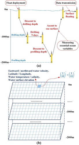
The HYCOM global assimilation data used in this study provided higher temporal and spatial resolutions than those provided by most previously adopted global assimilation model data, rendering them ideal data for modeling and analyzing global ocean circulation. The system uses the NCODA system for data assimilation (please refer to Appendices C and D for a more detailed introduction to the retrieval of model-initialized information from a climatological dataset and the data types assimilated in HYCOM + NCODA, respectively). NCODA uses the 24-hour model forecast as a first guess in a 3D variational scheme and assimilates available satellite altimeter observations, satellite, and in situ sea surface temperature as well as in situ vertical temperature and salinity profiles from XBTs, Argo floats, and moored buoys (Cummings and Smedstad 2013). With a horizontal grid resolution of 1/12° and 41 layers in the vertical direction, the HYCOM reanalysis dataset provided comprehensive information on key ocean variables such as temperature, salinity, sea surface height, and current velocity (de Souza et al. 2021). The HYCOM analysis and reanalysis data of the 3-hourly flow field for the global ocean from 2010 to 2022, obtained from the Thematic Real-time Environmental Distributed Data Services (THREDDS) data server, were utilized in this study (https://tds.hycom.org/thredds/catalog.html). HYCOM is a widely used Ocean General Circulation Model (OGCM) that incorporates wind stress and Coriolis forces but neglects Stokes drift (Gouillon 2010). Moreover, Global Ocean Forecasting System (GOFS) 3.1 analysis utilizes NAVGEM data as the wind force, relying on 3-hourly fields derived from the naval global atmospheric prediction system (Metzger et al. 2017). In contrast, GOFS 3.1 reanalysis utilizes the wind force obtained from CFSR and CFSv2, which provide hourly data (Yu, Fan, and Metzger 2022).

To ensure consistency with the maximum dive depth of the Argo float and accurately simulate the subsurface flow field, this study employed a total of 36 vertical levels of global HYCOM simulations ranging from the sea surface to a depth of 2,000 m (Figure 1(b)). The vertical resolution of these simulations included layers at 0, 2, 4, 6, 8, 10, 12, 15, 20, 25, 30, 35, 40, 45, 50, 60, 70, 80, 90, 100, 125, 150, 200, 250, 300, 350, 400, 500, 600, 700, 800, 900 m, 1,000 m, 1,250 m, 1,500 m, and 2,000 m. This selection of vertical layers enabled precise simulation of the flow field, which was essential for obtaining reliable and accurate results for the study.

2.2. Methods

The experimental design in this paper aimed to explore the spatial matching patterns between the Argo observed data and the HYCOM simulated data. This study aimed to uncover the rules governing the compatibility between datasets by examining systematic errors existing between data from various dimensions and perspectives, as well as performance patterns in different regions. Ultimately, this paper’s goal was to improve the accuracy and reliability of oceanographic models through a better understanding of the compatibility between observed and simulated data.

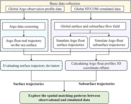
Figure 2 illustrates the following steps involved in screening the Argo dataset, evaluating surface trajectory deviation, and calculating the surface position distance error using both the Argo and HYCOM datasets. The study employed a dual approach to evaluate the performance of the HYCOM model, which involved comparing the model results with the Argo observations on the sea surface and using the Argo floats as particles to simulate their movements in the HYCOM subsurface flow field. These steps were implemented to ensure the accuracy and reliability of the experiment’s results.

Figure 2. Research framework.

2.2.1. Argo dataset screening

Argo has revolutionized the collection of information from within the oceans, which provides necessary data support for ocean environmental modeling. Argo floats adjust their buoyancy after deployment to descend to a depth of 1000 m and remain there for 5–9 days before descending further to 2000 m (Simon 2020). As the float ascends, it measures various elements of seawater using its built-in sensors. Once the float reaches the surface, it transmits observation data to satellites and uses an antenna to locate itself. After data transfer completion, the float again descends, and the cycle is repeated.

While most floats are programed to drift at depths of 1,000 m, some are set to shallower depths, such as 500 m or 800 m, particularly in marginal seas (Abraham et al. 2013). When a float rises to the surface, multiple satellite fixes are performed to ensure that all data are transmitted, often exceeding ten fixes. The float’s internal clock is used to time various operations, such as the time AET when it first reaches the surface and the time DST when it begins its descent after transmitting data, as shown in Figure 3.

Figure 3. Argo float complete motion trajectory (LLT: last location time; DST: descent start time; AST: ascent start time; AET: ascent end time; FLT: first location time).

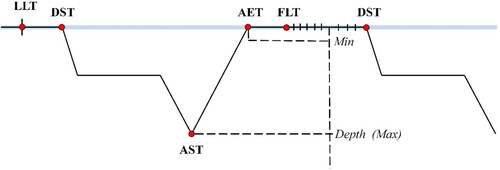
To simulate the float’s 3D motion trajectory in the HYCOM flow field, access to all-time float nodes at and below the sea surface was necessary. Therefore, the global Argo float data were first screened to include track files with the five-time point information of last location time (LLT), DST, ascent start time (AST), AET, and first location time (FLT) (Ollitrault and Rannou 2013). Additionally, the cycle number, time, time quality control marker, and satellite positioning accuracy of each float must be extracted for screening. Data with positioning time QC markers of 1 and 2 were chosen, with 1 indicating good data and 2 indicating possibly good data (Wong, Keeley, and Carval 2020). Metadata files for each float were also obtained to determine the drift depth.

2.2.2. Calculation of Argo float surface and subsurface trajectories

The trajectory of an Argo float on the sea surface was defined by a series of localization points obtained from its positioning system. This can be represented mathematically by Equation (1(1) $Tra{j}_{sur}=\{S{L}_1,\cdots ,S{L}_n\}$(1) ): (1) $Tra{j}_{sur}=\{S{L}_1,\cdots ,S{L}_n\}$(1) where $Tra{j}_{sur}$ denotes the coordinate sequence comprising the actual localization points of the Argo float on the sea surface, and the trajectory is obtained by connecting these points, $S{L}_1$ denotes the first localization point of a certain profile of the Argo float on the sea surface, and $\mathrm{S}{L}_n$ denotes the second localization point of a certain profile of the Argo float on the sea surface.

In the simulation of the Argo float’s motion in the HYCOM flow field of the sea surface, the float was regarded as a particle point. To increase the sampling rate of the simulated trajectory points, interpolation can be applied to generate smoother and finer simulated trajectories. The interpolation process employs the inverse distance weighting (IDW) method in the spatial domain (Ghomlaghi, Nasseri, and Bayat 2022). Initially, the Euclidean distance between the discrete points and the interpolation points was calculated.

At the second step, the weight $W_i$ of each point was calculated. The weight was determined as a function of the reciprocal of the distance. This parameter can be calculated as follows: (2) $W_i={\displaystyle \frac{{\left({\displaystyle \frac{1}{d_i}}\right)}^2}{{\sum }_{i=1}^n{\left({\displaystyle \frac{1}{d_i}}\right)}^2}}$(2) where $n$ is the total number of discrete points, and $d_i$ is the Euclidean distance between the discrete and interpolation points.

Finally, the value of the interpolation point was calculated as follows: (3) $z_0=\sum _{i=1}^n{W}_i\times Z(X_i,Y_i)$(3) Upon IDW interpolation of the simulated sea surface trajectory points, the resultant set of interpolated coordinate points was denoted as $\{P_i,\cdots ,P_n\}$. These points can be obtained as follows: (4) $\{\begin{array}{c}{P}_i=(X_i,Y_i)\\ X_i=\sum _{i=1}^n{u}_i\times t,t=10min,1\le i\le n\\ Y_i=\sum _{i=1}^n{v}_i\times t,t=10min,1\le i\le n\end{array}$(4) where $i$ is a simulated point, which is a positive integer, and $n$ denotes the total number of Argo float sea surface trajectory points in a certain section. $P_i$ denotes the coordinates of a simulated trajectory point, and $u_i$ and $v_i$ denote the eastward and northward velocities, respectively, of seawater at point $i$ in the HYCOM sea surface current field.

The original temporal resolution of the HYCOM data is 3 h (de Faria, de Queiroz, and DeCarolis 2022). However, the positioning time of Argo floats on the sea surface can vary from a few minutes to several hours. To match the actual moving process of Argo floats on the sea surface more accurately, the temporal resolution was increased to 10 min via linear interpolation.

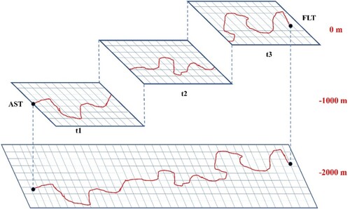
In simulating the movement of an Argo float in the HYCOM ocean 3D dynamic field, the float was also treated as a particle. The simulation began at the position where the Argo float began ascending to the sea surface (AST), and the $u$ and $v$ velocity values in the HYCOM ocean 3D dynamic field were utilized to calculate the Argo float three-dimensional movement trajectory. As the HYCOM model adopted grid division in the horizontal direction and multiple layers in the vertical direction, the movement trajectory of the Argo float had to be simulated separately in the horizontal grids of different depths.

To obtain the magnitude and direction of the zonal velocity $u$ and meridional velocity $v$ stored in the current cell, the float accessed each grid cell entered. The float moved in the direction of the current until it entered the next cell and then changed its movement direction. This process was repeated until the float reached the surface at the FLT moment. The simulation process can be visualized in Figure 4. Finally, the deviation of the profile 3D coordinates of the float simulated by the HYCOM underwater flow field from the initial coordinates positioned at the sea surface was calculated.

Figure 4. Simulation of the Argo float motion in the HYCOM subsurface flow field.

2.2.3. Evaluation of the trajectory deviation degree

The trajectory deviation degree (TDD) evaluation method was used to assess the performance of the HYCOM sea surface flow field. It involved comparing the observed trajectories of Argo floats and simulated trajectories of the HYCOM flow field at the sea surface. In the TDD evaluation method, the average degree of the difference in the simulated and observed distances between the float locations over the specified period was calculated. This measure of trajectory deviation is primarily based on the definition of the distance between trajectory points, which is expressed using the matching degree between points (Ahmed, Chun-Wei Lin, and Srivastava 2023). In this study, the distance between the corresponding moment points in two trajectories was used to determine the trajectory deviation (Figure 5), and the evaluation of the travel distance and direction of the flow velocity has been implicitly included (please refer to Appendix E for a more detailed introduction to the length and angle deviation results between the real and simulated Argo profile sea surface trajectories).

Figure 5. Trajectory deviation evaluation method.

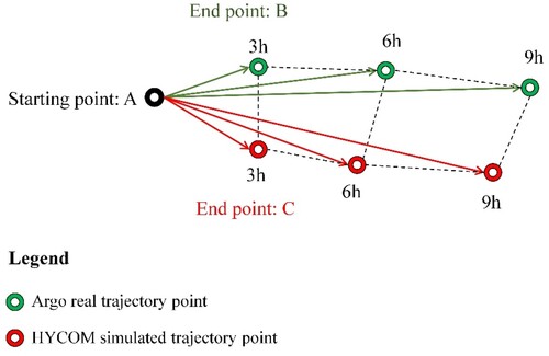
First, the deviation distance of the corresponding moment points of the two trajectories was calculated separately. After obtaining the deviation values of the coordinate points on each trajectory at various moments, the results were summed and averaged to obtain the deviation results between trajectory AB and trajectory AC. The closer the two trajectories were, the smaller the deviation value. Conversely, a greater deviation value indicated dissimilarity between the two trajectories. The trajectory deviation evaluation method is presented in Equation (5(5) $TDD={\displaystyle \frac{B{C}_{dis}}{A{B}_{dis}+A{C}_{dis}+B{C}_{dis}}}$(5) ): (5) $TDD={\displaystyle \frac{B{C}_{dis}}{A{B}_{dis}+A{C}_{dis}+B{C}_{dis}}}$(5) where $B{C}_{dis}$ denotes the distance between two points $B$ and $C$, $A{B}_{dis}$ denotes the distance from the current moment point $B$ to the start point $A$, $A{C}_{dis}$ denotes the distance from the current moment point of trajectory $C$ to the start point $A$, and $TDD$ denotes the ratio of the distance $B{C}_{dis}$ between two trajectory points at the same moment to the total cumulative length of $A{B}_{dis}$, $A{C}_{dis}$, and $B{C}_{dis}$.

After calculating the deviation degree of each point of the two trajectories, the deviation degree between these two trajectories can be obtained: (6) $Traj\mathrm{\_}dev={\displaystyle \frac{TD{D}_1+\cdots +TD{D}_n}{TD{D}_{num}}}$(6) $Traj\mathrm{\_}dev$ is the deviation degree of the two trajectories. The lower $Traj\mathrm{\_}dev$ is, the closer the two trajectories.

2.2.4. Analysis of the three-dimensional coordinate distribution

This paper presents a statistical analysis of the three-dimensional coordinates of the Argo float obtained during ascent sampling of the HYCOM subsurface flow field, along with the initial sea surface positioning coordinates. By analyzing the distribution of the coordinates and the offset range, statistical analysis can provide a more comprehensive visualization of the data. The approach for conducting statistical analysis is depicted in Figure 6.

Figure 6. Spatial and statistical analysis process.

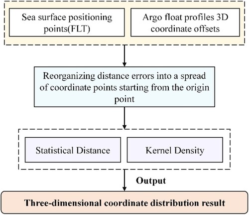
These errors were reorganized into a spread of coordinate points that started from the origin point and expanded in all directions. Then, the statistical analysis method was employed to measure the concentration or dispersion of features around the origin point. A buffer circle was drawn based on the distribution of the distance error, and the overall data distribution was determined based on the number of enclosed points. The first buffer circle encompassed approximately 98% of the coordinate points, and the second buffer circle comprised approximately 99% of the coordinate points. The statistical distance can be calculated as follows: (7) $SD=\sqrt{{\displaystyle \frac{{\sum }_{i=1}^n{(x_i-0)}^2}{n}+{\displaystyle \frac{{\sum }_{i=1}^n{(y_i-0)}^2}{n}}}}$(7) where $x_i$ and $y_i$ are the coordinates of element $i$, and $n$ is the total number of elements. Then, the radius was calculated to determine the error of the 3D coordinate offsets of the Argo float profiles.

Finally, kernel density (KD) analysis was used to determine the density of the coordinate point offsets of the Argo 3D trajectory (Song, Prishchepov, and Song 2022). KD analysis is a spatial statistical technique for estimating point data density in geographic space. It entails using a kernel function to smooth the density of points and identifying areas of high and low density by performing KD analysis on 3D coordinate points. A kernel function is a mathematical function used in KD estimation to estimate the probability density function of a random variable. It was used to smooth out the data and obtain a continuous probability density function. The kernel function determined the shape of the estimation curve, and the bandwidth determined the variation in the density estimates. The kernel function can be expressed as follows (Silverman 1986): (8) $k_n={\displaystyle \frac{1}{nr}\sum _{i=1}^{n}k\left({\displaystyle \frac{p-p_i}{r}}\right)}$(8) where $k_n$ denotes the KD value of the spatial distribution of the 3D coordinates of the Argo float profiles; $n$ is the number of coordinate points, $k$ is the function of KD measurements; $p-p_i$ denotes the distance between the coordinate points, and $r$ is the search radius.

3. Results

3.1. Screening results for the global Argo float profile data

The study obtained 17,649 Argo floats globally from February 2010 to November 2022, resulting in several million profiles. To ensure data accuracy, the profiles underwent a meticulous screening process, which eliminated any missing information on underwater time. Consequently, each profile included the required parameters, namely, LLT, DST, AST, AET, and FLT. Following the screening process, the study retained 397,246 original sea surface positioning points for further analysis. The final dataset encompassed a vast majority of ocean basins, as illustrated in Figure 7.

Figure 7. Original sea surface localization points of Argo (February 2010 to November 2022).

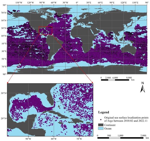
Based on the data screening results, not all sea areas are covered by Argo floats, such as the South China Sea, Japan Sea, and North Pacific Ocean. This occurs because the subsurface float time information (LLT, DST, AST, AET, and FLT) is needed in the experiment, and Argo profiles without underwater time data were excluded in advance. Moreover, the polar regions exhibited a lower density of float data due to the original design of the global Argo array, which was intended for open ocean areas and did not encompass seasonal sea ice and marginal seas. Nonetheless, Argo is expanding its global coverage to encompass these areas, which were initially excluded owing to technological restrictions.

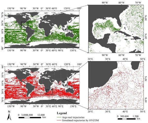
3.2. Matching results of simulated and observed data in the sea surface flow field

The eastward and northward seawater velocity values from the HYCOM model were utilized to verify the accuracy of its sea surface current flow field by calculating the position of the same moment as the Argo float’s positioning point on the sea surface. These calculated points were then connected to obtain the simulated trajectory of the float in the sea surface flow field, resulting in a total of 200,900 surface simulation trajectory points and 191,136 surface simulation trajectories globally (Figure 8). A total of 193,498 real drift tracks of the floats on the sea surface were obtained after connecting the Argo float’s real positioning points between time FLT and time DST on the sea surface. However, due to some missing data in the HYCOM simulation results, the number of float sea surface motion trajectories that were simulated using the HYCOM model was found to be less than the actual trajectories of the floats at the sea surface. Notably, there are times when the daily Global Ocean Forecast System may not run due to computer issues, problematic input data sources, or other unforeseen problems.

Figure 8. Original and simulated trajectories of global Argo floats on the sea surface.

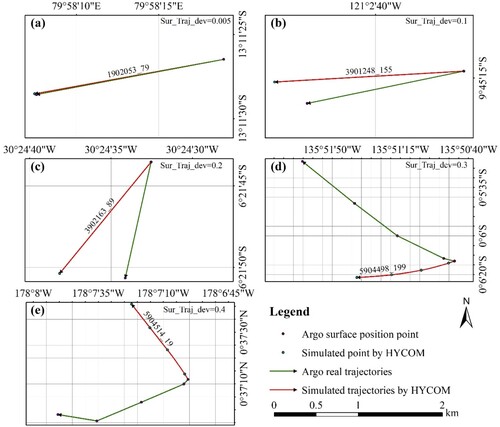
The deviation degree between the real trajectory of Argo floats on the sea surface and the trajectory simulated by the HYCOM surface flow field ranged from 0 to 0.5. Figure 9 shows selected trajectories with different deviation degrees. As shown in the graph, higher deviation degrees resulted in less similarity between the two trajectories, while lower deviation degrees resulted in greater similarity. A deviation degree less than 0.2 was considered indicative of essentially similar trajectories. Notably, the magnitude and direction of the flow velocity in the flow field may change over time. Therefore, the simulated trajectory results became smoother and finer after spatiotemporal interpolation of the HYCOM sea surface flow field.

Figure 9. Results for the different deviation degrees between the real and simulated trajectories of Argo floats on the sea surface; (a) deviation degree=0.005; (b) deviation degree=0.1; (c) deviation degree=0.2; (d) deviation degree=0.3; (e) deviation degree=0.4.

To visualize and analyze the deviation degree between trajectories, the global sea area was divided into a 2° × 2° grid, as presented in Figure 10. The degree of similarity between trajectories characterized the accuracy of the HYCOM surface flow field. The deviation value increased as the similarity decreased. Conversely, the deviation value decreased as the similarity increased. The deviation degree results were distributed in a band with the equator as the axis and north‒south symmetry. In general, the sea surface trajectory deviation was lower at higher latitudes, indicating that the HYCOM surface current field data at high latitudes were less accurate than the Argo observations.

Figure 10. Deviation between the Argo float sea surface real trajectories in a global 2°×2° grid and the trajectories simulated using the HYCOM surface flow field.

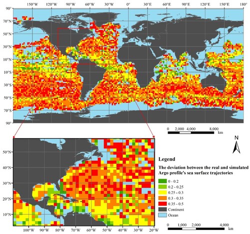
According to Table 1, trajectories with deviation values greater than 0.3 constituted 58% of the total global trajectories, with most of them distributed in mid- and high-latitude sea areas. These results suggested that the HYCOM surface current fields in these regions were not accurate enough. However, in low-latitude regions, the deviation values were generally less than 0.2, and the grid deviation values are shown in green, indicating that the trajectories were similar. Moreover, 23% of trajectories had deviation degree values between 0.2 and 0.3, which meant that they were fairly similar. Nineteen percent of all global trajectories had deviation degree values less than 0.2, indicating a small number of similar trajectories. Notably, the accuracy of the HYCOM surface current flow field near the equator was relatively high, as demonstrated in Figure 9(a). The simulated trajectory closely aligned with the actual motion of the Argo float at the sea surface.

Table 1. Percentage of the different trajectory deviation degree intervals.

Deviation degree interval (%)	Percentage (%)
0 ≤ Traj_dev < 10	5
10 ≤ Traj_dev < 20	14
20 ≤ Traj_dev < 30	23
30 ≤ Traj_dev < 40	26
Traj_dev ≥ 40	32

3.3. Matching results of the simulated and observed data in the subsurface flow field

The measurement cycle of an Argo float typically lasted approximately 10 days, whereas it spent the majority of its time below the sea surface and a few to a dozen hours at the surface for positioning. Therefore, to accurately simulate the trajectory of Argo floats below the surface, a high spatial and temporal resolution 3D dynamic field of the ocean was essential. Floats with surface trajectory deviations less than 0.2 were selected to simulate their underwater 3D motion trajectories. In the HYCOM underwater flow field model, the Argo float was considered a point particle. Its 3D coordinates were calculated as it ascended from a depth of 2,000 m to the surface. The resulting coordinates were then organized into a circular distribution centered at the origin point, allowing for a more visually intuitive representation of the error between the 3D coordinates and the sea surface location (FLT). To quantify the geographic distribution of all Argo float profiles’ 3D coordinates and the farthest points from the surface first location point (FLT), the statistical distance was conducted, as shown in Figure 11.

Figure 11. Statistical distance distribution of the 3D coordinate points of the Argo float profiles; (a) buffer cycle of all coordinate points of each Argo profile; (b) buffer cycle of the farthest coordinate points of each Argo profile.

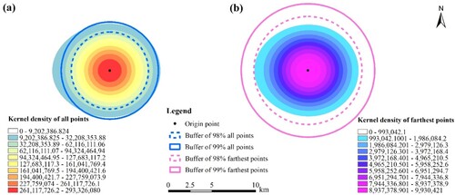
Statistical analysis revealed that the deviation between the 3D coordinates for 98% of the profiles and the location at FLT time was less than 4.43 km, while the deviation between the 3D coordinates for 99% of the profiles and the location at FLT time was less than 5.58 km (Figure 11(a)). Furthermore, statistical analysis of the farthest points in the 3D coordinates of each profile showed that the deviation of the coordinates for 98% of the farthest points from the location at FLT time was approximately 5.73 km, while the deviation of the coordinates for 99% of the farthest points from the location at FLT was approximately 7.07 km (Figure 11(b)). These findings suggested a considerable deviation from the location at the FLT among the farthest points. Based on the coordinate point distribution data, we chose 5,000 m as the radius parameter for KD calculation to have a radius value that was neither too large nor too small for coordinate point aggregation. From the results of KD analysis, the distribution of 3D coordinate points in the Argo profile was more concentrated. The coordinate points were more densely distributed in the origin point and less distributed in the peripheral area, showing a circular diffusion distribution from the origin point to the surrounding area.

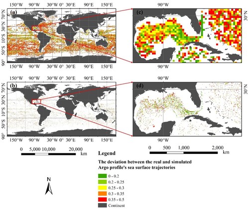
The global ocean was divided into a 2° × 2° grid to visualize the deviation of the 3D coordinates of the Argo profiles, as shown in Figure 12. The results demonstrated that the offset of the float 3D coordinates was greater in some mid-latitude areas. Specifically, in the Northern Hemisphere, the 3D coordinate offset was highest in the region extending from the Gulf Stream to the warm North Atlantic Current, ranging from 30° W to 90° W longitude and 20° N to 50° N latitude. In the Southern Hemisphere, a clear pattern emerged wherein the area with a larger offset was distributed in red stripes along the westerly drift, from west to east, between 180° W to 180° E longitude and 30° S to 60° S latitude.

Figure 12. Horizontal distance from the float position at the maximum profiling depth (time: AST; simulated coordinates by the HYCOM subsurface flow field) to the first location position (time: FLT; real coordinates by satellite positioning) at the surface in a global 2°×2° grid.

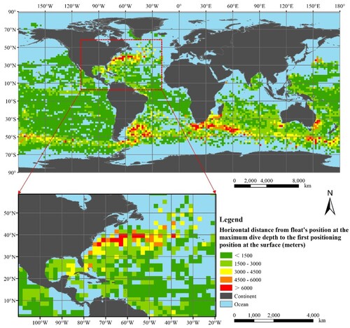
The analysis indicated that 10% of the global ocean area had a 3D coordinate offset exceeding 3 km, while 90% of the 3D coordinate offsets in the global ocean were less than 3 km, as shown in Table 2. The validation results of the flow field below the sea surface corresponded with those of the surface flow field, and the HYCOM 3D flow field accuracy was lower in mid-latitude waters.

Table 2. Percentage of the 3D coordinate offsets of the Argo float profiles.

Argo float profile 3D coordinate offset interval (m)	Percentage (%)
0 ≤ offset < 3000	90
3000 ≤ offset < 6000	8
offset ≥ 6000	2

4. Discussion

4.1. Effect of different grid scales on the analysis results

The accuracy and level of detail of the data obtained from the sea surface current field were affected by the resolution of the sea area grid. Choosing different resolutions may lead to varied research results and influence the speed and efficiency of calculations. It is therefore essential to select the appropriate resolution size for gridding the global sea area, considering the research objectives and data characteristics and exploring the differences and effects of various resolutions on the research results.

Lower resolution grids under a global view could quickly uncover the distribution of sea surface current field data errors on a macroscopic scale, as shown in Figure 13(a), where the grid resolution was 5°×5°. The grids clearly illustrated that the degree of deviation between sea surface trajectories was symmetrically distributed with increasing latitude on the equator axis. The coverage of the sea area increased as the grid resolution decreased. This resulted from averaging the deviation degree values of the sea surface trajectory when the deviation degree between the grid and the sea surface trajectory was spatially connected. When the grid resolution was low, the surface that intersected with the deviation degree value did not represent the deviation degree value, so less area was covered.

Figure 13. Deviation degree of the sea surface trajectory in the grids with different resolutions under a global view; (a) 5°×5° global grid; (b) 2°×2° degree global grid; (c) 1°×1° degree global grid.

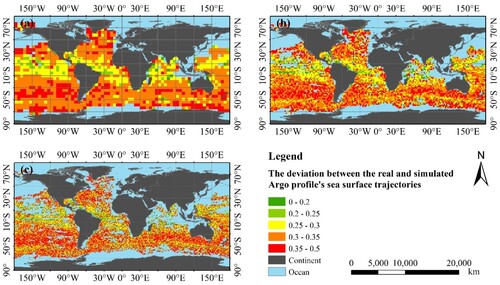
However, using a low-resolution grid may ignore some locally detailed features. In contrast, a higher-resolution grid can provide more spatial detail and accuracy, which is vital for capturing small-scale features and processes. The 2° × 2° grid could consider spatially detailed features while ensuring that the basic features of the currents were evident on the global scale, as shown in Figure 13(b). On the other hand, at a resolution higher than 2°×2°, the general pattern of ocean currents in spatial distribution was not obvious at the global scale, leading to an inability to analyze accurately at the macroscopic level, as shown in Figure 13(c). In the area of a high sea surface flow velocity, the classification interval of the visualization results of the deviation rate of the sea surface trajectories changed with grid resolution. Therefore, the grid resolution can be increased in areas of focus to capture more detail, while in other regions, it can be appropriately reduced to optimize computational resources and time.

When the grid resolution was too high, the variability characteristics of the sea surface flow field could not be analyzed from the global scale, and only local analysis could be performed, as shown in Figure 14(a,b). From the regional perspective, the accuracy of the HYCOM sea surface current field was high in the region where the currents were more rapid. For instance, the results of the sea surface current field of the Gulf Stream were consistent with the real ocean current pattern, as shown in Figure 14(c,d).

Figure 14. Deviation degree of the sea surface trajectory in the grids with different resolutions under a local view; (a) and (c) 0.5°×0.5° degree global grid; (b) and (d) 0.08°×0.08° degree global grid.

4.2. Error pattern analysis of the HYCOM flow field data performance

Analyzing the differences between model simulation data and observation data can help to improve the accuracy of the simulation model. The experimental results indicated that there were regional disparities in the simulation of sea surface trajectories. Regions with a poor deviation of sea surface trajectories were primarily situated in the areas of the West Wind Drift and Western Boundary Current. Ocean circulation is conceptually divided into two parts: wind-driven rapidly changing surface circulation (wind-generated circulation) and slowly changing deep circulation driven by the thermohaline field (density field) (Neumann 1968; Reader 2022).

In the upper layers of the world ocean, where the depth is shallower than 1,000 m, the circulation is primarily driven by wind stress. The West Wind Drift is an oceanic current that flows latitudinally from west to the east in the vast ocean near 40°−60°S under the influence of prevailing westerly winds. As the west wind blows across the sea surface, it generates friction with the surface of the sea and applies pressure on the windward side of the waves, resulting in the seawater being propelled forward. Once the surface seawater starts to move, the geostrophic deflection and friction forces come into effect (de Lavergne et al. 2022). Westerly drift is formed when the wind-driven currents are balanced by the geostrophic deflection force, the frictional force of the underlying seawater, and the wind, causing the currents to reach a steady state and flow forward at an equal speed (Schott and McCreary 2001). The Western Boundary Current is an oceanic current that flows along the boundaries of the oceans and is driven by wind (Hu et al. 2015). The Gulf Stream, which flows northward along the east coast of the United States and diverges at 45°N and 45°W, with all its branches collectively known as the North Atlantic Warm Current, is the most typical example of this type of current. Therefore, the poor performance of the HYCOM model in simulating the sea surface current field data in these regions may have been influenced by surface winds.

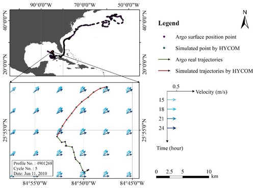
The performance of the HYCOM surface flow field was further evaluated by visualizing the magnitude and direction of the flow field based on the data’s temporal resolution. As shown in Figure 15, the magnitude and direction of the flow velocity of the flow field changed every 3-hour interval. Consequently, the simulated trajectory direction changed accordingly with the magnitude and direction of the flow velocity. Compared to the HYCOM simulated trajectory, the real trajectory of the Argo sea surface was composed of a series of satellite positioning points on the sea surface, which was more realistic. However, the simulation results of the model were not actual observation data. Improving the accuracy of the model simulation was the objective, as it was not possible to make it identical to the actual measurement data. Nonetheless, there is a possibility that the simulation results were not accurate in certain areas due to various circumstances. This may result in a situation where the simulated trajectory direction of the sea surface is opposite to the real trajectory direction of Argo.

Figure 15. Difference between the real and simulated sea surface trajectories of the 5th profile of float number 4901268 (Data: 11 June 2010).

The current Argo floats only provided measurements during the process of ascending to the surface, which means that each ocean element’s information is only partially recorded. Therefore, this study used HYCOM underwater flow field data to simulate the spatial coordinates of global Argo floats from 2,000 m below sea level to the surface. However, there was a partial offset between the 3D coordinates of the Argo profile calculated by the HYCOM underwater flow field data and the coordinates of the float positioning at the sea surface, and this offset varied regionally. After an investigation, it was discovered that the global HYCOM analysis and reanalysis dataset do not incorporate tides. However, the inclusion of a coastal model nested into HYCOM on its open boundaries could introduce tidal forcing.

However, the role of tides in deep ocean mixing cannot be ignored, especially in areas with rough seafloor topography (e.g. seamounts, trenches, and ridges), where tidally induced internal wave fragmentation mixing plays an important role (de Lavergne et al. 2020; Geoffroy and Nycander 2022). Integrating tides into the ocean model can alter the model morphological structure of the oceanic deep circulation and enhance the deep current velocity (Allen and Durrieu de Madron 2009; Su et al. 2023). Therefore, the influence of tides should be considered in deep circulation simulation (Melet, Hallberg, and Marshall 2022). Another possible explanation is that the assimilation of global HYCOM model data may alter the dynamic characteristics of the model, disrupting the flow field at and below the sea surface. Consequently, there are numerous uncertainties associated with the current HYCOM model in simulating the deep flow field, which may account for the significant discrepancies between the simulated 3D coordinates of the Argo float profile and the sea surface localization points.

4.3. Limitations and future research directions

The combination of the HYCOM model with Argo measured data is a promising approach to improve the accuracy of the HYCOM model data, but it also has certain limitations and requires further research to enhance its effectiveness. One limitation of this approach is the limited spatial and temporal coverage of the Argo floats. Although the number of floats has increased significantly in recent years, there are still gaps in coverage, especially in remote areas of the ocean (Kim et al. 2023). In addition, the data obtained by Argo floats are mostly at the surface or at depths up to 2,000 m, which may not fully capture the vertical structure of the ocean. Future research could focus on improving the spatial and temporal resolution of Argo floats by increasing their numbers or developing new sensors. Another limitation is that the HYCOM model is based on mathematical equations and assumptions, which may not fully represent the complexity of the real ocean. Therefore, the accuracy of the model may be limited in certain regions or under certain conditions, such as near the coastline or in areas with complex topography. The HYCOM model is a numerical ocean model that can be used to simulate the three-dimensional velocity and various properties of the ocean by incorporating several key physics components. These components, including the Navier‒Stokes equations, advection, turbulence, buoyancy effects, bottom topography, forcing mechanisms, and parameterizations, are highly important in determining the modeled velocity and its comparison to the observed velocity. The HYCOM model configuration for surface forcing encompasses factors such as wind stress, wind speed, thermal forcing, precipitation, and relaxation to the climatological sea surface salinity (SSS). Despite the inclusion of these physics components, discrepancies between modeled and observed velocities can still arise due to various factors. These factors may involve inaccuracies in model initialization, uncertainties in boundary conditions, limitations of the spatial and temporal resolutions, and errors in the input data or parameterizations.

Additionally, when visualizing the results, the choice of classification method can significantly influence the analysis of the findings. This study used a fixed interval method to classify the experiments to better show the distribution of data in different threshold intervals. This classification method can flexibly adjust the data in intervals and classify them according to actual needs. However, this method has some disadvantages, such as not being suitable for classifying outliers, and may result in insufficient data in some intervals and excessive data in others, making it difficult to distinguish them. This paper discusses the simulation of the float’s motion in a flow field, specifically the Argo float, which is treated as a particle. However, the analysis is limited to the float’s ascending and floating phases, and the 3D coordinates of the float during its diving and stationary phases are not considered. The reason for this is that the Argo float is primarily used to measure ocean element data during its ascent process. To enhance the evaluation of the HYCOM flow field, it is crucial to simulate the entire underwater motion of the Argo particle in future studies. This would involve incorporating the float’s diving and stationary phases into the calculation of its 3D coordinates. This approach would provide a more comprehensive understanding of the flow field and could lead to improved simulations. Future research could focus on enhancing the accuracy of the model by incorporating more detailed and comprehensive data. In addition, various data combination methods, including data assimilation techniques, could be explored to evaluate the performance of HYCOM data.

5. Conclusions

In this paper, the performance of the HYCOM model in simulating global ocean currents was investigated by combining Argo observations with a HYCOM-provided flow field. By mining the spatial matching pattern between the model data and observations, the differences in the sea surface and underwater current field data performance of the model in different regions were revealed. The main study conclusions are as follows: (1) the HYCOM surface and subsurface flow fields generally conformed to the basic characteristics and trends of ocean currents. However, the simulation of the surface current field was affected by wind, while the simulation of the deep current field was influenced by tides. (2) Comparing the real trajectories of Argo floats at the sea surface with the HYCOM sea surface flow field, it was found that 19% of the sea surface trajectories exhibited a high degree of similarity, while 23% of the trajectories were largely similar. In contrast, 58% of the trajectories showed low similarity. Furthermore, the accuracy error of the HYCOM sea surface flow field was centered on the equator and increased with increasing latitude. (3) The profile 3D coordinate offsets of the Argo float particles were calculated in the HYCOM subsurface 3D flow field, and it was determined that 90% of the 3D coordinate offsets were less than 3 km, while the remaining 10% of the offsets ranged from 3 to 18.3 km. The accuracy of the HYCOM subsurface flow field varied by region, with larger offsets in the Gulf Stream, North Atlantic Warm Current, and West Wind Drift regions.

Ocean simulation data and observations are crucial for many digital Earth applications, including weather forecasting, climate modeling, and oceanographic research. The ocean is a complex system, and understanding its dynamics is essential for predicting the planet’s future climate and the impacts of climate change. By including ocean simulation data and observations in the digital Earth, scientists can better understand and manage the impacts of human activities on the ocean. Matching analysis between Argo observations and HYCOM model data plays a crucial role in constructing a digital Earth system. The study results provide valuable insights into the performance of the HYCOM model in simulating complex oceanic systems, including surface currents and subsurface flow fields. Furthermore, by identifying the factors that contribute to the errors between the simulated and observed data, this study could enhance the utilization of HYCOM simulation data and support future research on HYCOM model improvement.

Acknowledgements

We appreciate the detailed suggestions and comments from editors and anonymous reviewers.

Disclosure statement

No potential conflict of interest was reported by the author(s).

Data availability statement

The global Argo float data are provided by the International Argo Program and relevant contributing countries (ftp://data.argo.org.cn/pub/ARGO/raw_argo_data/). The HYCOM analysis and reanalysis data in this study are available at https://tds.hycom.org/thredds/catalog.html.

Additional information

Funding

This work was supported by National Natural Science Foundation of China [grant nos: 41930648, 42171406 and 42171465]; National Key Research and Development Program of China [grant no: 2021YFB3900901].

References

- Abraham, J. P., M. Baringer, N. L. Bindoff, T. Boyer, L. J. Cheng, J. A. Church, J. L. Conroy, et al. 2013. “A Review of Global Ocean Temperature Observations: Implications for Ocean Heat Content Estimates and Climate Change.” Reviews of Geophysics 51 (3): 450–483. https://doi.org/10.1002/rog.20022.
- Agarwal, Neeraj, Rashmi Sharma, and Raj Kumar. 2022. “Impact of Along-Track Altimeter Sea Surface Height Anomaly Assimilation on Surface and Sub-Surface Currents in the Bay of Bengal.” Ocean Modelling 169:101931. https://doi.org/10.1016/j.ocemod.2021.101931.
- Ahmed, Usman, Jerry Chun-Wei Lin, and Gautam Srivastava. 2023. “Deep Fuzzy Contrast-set Deviation Point Representation and Trajectory Detection.” IEEE Transactions on Fuzzy Systems 31 (2):571–581. https://doi.org/10.1109/TFUZZ.2022.3197876.
- Allen, S. E., and X. Durrieu de Madron. 2009. “A Review of the Role of Submarine Canyons in Deep-Ocean Exchange with the Shelf.” Ocean Science 5 (4):607–620. https://doi.org/10.5194/os-5-607-2009.
- Annoni, Alessandro, Stefano Nativi, Arzu Çöltekin, Cheryl Desha, Eugene Eremchenko, Caroline M. Gevaert, Gregory Giuliani, et al. 2023. “Digital Earth: Yesterday, Today, and Tomorrow.” International Journal of Digital Earth 16 (1):1022–1072. https://doi.org/10.1080/17538947.2023.2187467.
- Brokaw, Richard J., Bulusu Subrahmanyam, Corinne B. Trott, and Alexis Chaigneau. 2020. “Eddy Surface Characteristics and Vertical Structure in the Gulf of Mexico from Satellite Observations and Model Simulations.” Journal of Geophysical Research: Oceans 125 (2):e2019JC015538. https://doi.org/10.1029/2019JC015538.
- Chamberlain, Paul M., Lynne D. Talley, Matthew R. Mazloff, Stephen C. Riser, Kevin Speer, Alison R. Gray, and Armin Schwartzman. 2018. “Observing the Ice-Covered Weddell Gyre with Profiling Floats: Position Uncertainties and Correlation Statistics” Journal of Geophysical Research: Oceans 123 (11): 8383–8410. https://doi.org/10.1029/2017JC012990.
- Chassignet, Eric P., Harley E. Hurlburt, E. Joseph Metzger, Ole Martin Smedstad, James A. Cummings, George R. Halliwell, Rainer Bleck, Remy Baraille, Alan J. Wallcraft, and Carlos Lozano. 2009. “US GODAE: Global Ocean Prediction with the HYbrid Coordinate Ocean Model (HYCOM).” Oceanography 22 (2):64–75. https://doi.org/10.5670/oceanog.2009.39.
- Chassignet, Eric P., Harley E. Hurlburt, Ole Martin Smedstad, George R. Halliwell, Patrick J. Hogan, Alan J. Wallcraft, Remy Baraille, and Rainer Bleck. 2007. “The HYCOM (HYbrid Coordinate Ocean Model) Data Assimilative System.” Journal of Marine Systems 65 (1-4):60–83. https://doi.org/10.1016/j.jmarsys.2005.09.016.
- Chassignet, Eric P., Harley E. Hurlburt, Ole Martin Smedstad, George R. Halliwell, Alan J. Wallcraft, E. Joseph Metzger, Brian O. Blanton, Carlos Lozano, Desiraju B. Rao, and Patrick J. Hogan. 2006. “Generalized Vertical Coordinates for Eddy-Resolving Global and Coastal Ocean Forecasts.” Oceanography 19 (1):118–129. https://doi.org/10.5670/oceanog.2006.95.
- Chen, Min, Guonian Lv, Chenghu Zhou, Hui Lin, Zaiyang Ma, Songshan Yue, Yongning Wen, et al. 2021. “Geographic Modeling and Simulation Systems for Geographic Research in the new era: Some Thoughts on their Development and Construction.” Science China Earth Sciences 64 (8): 1207–1223. https://doi.org/10.1007/s11430-020-9759-0.
- Costa, F. B., and C. A. S. Tanajura. 2022. “On the Impact of Vertical Coordinate Choice for Innovation when Assimilating Hydrographic Profiles into Isopycnal Ocean Models.” Ocean Modelling 169:101917. https://doi.org/10.1016/j.ocemod.2021.101917.
- Cummings, J. A., and O. M. Smedstad. 2013. “Variational Data Assimilation for the Global Ocean.” In Chap. 13 in Data Assimilation for Atmospheric, Oceanic and Hydrologic Applications, Vol. II, edited by Seon Ki Park, and Liang Xu, 303–343. Berlin, Heidelberg: Springer.
- de Faria, Victor A. D., Anderson R. de Queiroz, and Joseph F. DeCarolis. 2022. “Optimizing Offshore Renewable Portfolios Under Resource Variability.” Applied Energy 326:120012. https://doi.org/10.1016/j.apenergy.2022.120012.
- de Lavergne, Casimir, Sjoerd Groeskamp, Jan Zika, and Helen L. Johnson. 2022. “The Role of Mixing in the Large-Scale Ocean Circulation.” In Chap. 3 in Ocean Mixing: Drivers, Mechanisms and Impacts, edited by Michael Meredith and Alberto Naveira Garabato, 35–63. Amsterdam: Elsevier.
- de Lavergne, C., C. Vic, G. Madec, F. Roquet, A. F. Waterhouse, C. B. Whalen, Y. Cuypers, P. Bouruet-Aubertot, B. Ferron, and T. Hibiya. 2020. “A Parameterization of Local and Remote Tidal Mixing.” Journal of Advances in Modeling Earth Systems 12 (5):e2020MS002065. https://doi.org/10.1029/2020MS002065.
- de Souza, Joao Marcos Azevedo Correia, Phellipe Couto, Rafael Soutelino, and Moninya Roughan. 2021. “Evaluation of Four Global Ocean Reanalysis Products for New Zealand Waters-A Guide for Regional Ocean Modelling.” New Zealand Journal of Marine and Freshwater Research 55 (1):132–155. https://doi.org/10.1080/00288330.2020.1713179.
- Dorfschäfer, G. S., C. A. S. Tanajura, F. B. Costa, and R. C. Santana. 2020. “A New Approach for Estimating Salinity in the Southwest Atlantic and Its Application in a Data Assimilation Evaluation Experiment.” Journal of Geophysical Research: Oceans 125 (9):e2020JC016428. https://doi.org/10.1029/2020JC016428.
- Franz, Guilherme, Carlos A. E. Garcia, Janini Pereira, Luiz Paulo de Freitas Assad, Marcelo Rollnic, Luis Hamilton P. Garbossa, and LetíCia Cotrim Da Cunha, et al. 2021. “Coastal Ocean Observing and Modeling Systems in Brazil: Initiatives and Future Perspectives.” Frontiers in Marine Science 8:681619. https://doi.org/10.3389/fmars.2021.681619.
- Gasparin, F., M. Hamon, E. Rémy, and P. Y. Le Traon. 2020. “How Deep Argo will Improve the Deep Ocean in an Ocean Reanalysis.” Journal of Climate 33 (1): 77–94. https://doi.org/10.1175/JCLI-D-19-0208.1.
- Geoffroy, Gaspard, and Jonas Nycander. 2022. “Global Mapping of the Nonstationary Semidiurnal Internal Tide Using Argo Data.” Journal of Geophysical Research: Oceans 127 (4):e2021JC018283. https://doi.org/10.1029/2021JC018283.
- Ghomlaghi, Arash, Mohsen Nasseri, and Bardia Bayat. 2022. “How to Enhance the Inverse Distance Weighting Method to Detect the Precipitation Pattern in a Large-Scale Watershed.” Hydrological Sciences Journal 67 (13):2014–2028. https://doi.org/10.1080/02626667.2022.2124874.
- Gouillon, Flavien. 2010. Internal Wave Propagation and Numerically Induced Diapycnal Mixing in Oceanic General Circulation Models. Tallahassee: University of Florida Press.
- Guo, Huadong, Dong Liang, Fang Chen, and Zeeshan Shirazi. 2021. “Innovative Approaches to the Sustainable Development Goals Using Big Earth Data.” Big Earth Data 5 (3):263–276. https://doi.org/10.1080/20964471.2021.1939989.
- Guo, Huadong, Zhen Liu, Hao Jiang, Changlin Wang, Jie Liu, and Dong Liang. 2017. “Big Earth Data: A new Challenge and Opportunity for Digital Earth’s Development.” International Journal of Digital Earth 10 (1): 1–12. https://doi.org/10.1080/17538947.2016.1264490.
- Hu, Dunxin, Lixin Wu, Wenju Cai, Alex Sen Gupta, Alexandre Ganachaud, Bo Qiu, Arnold L Gordon, et al. 2015. “Pacific Western Boundary Currents and their Roles in Climate.” Nature 522 (7556): 299–308. https://doi.org/10.1038/nature14504.
- Johnson, Gregory C., Shigeki Hosoda, Steven R. Jayne, Peter R. Oke, Stephen C. Riser, Dean Roemmich, Tohsio Suga, Virginie Thierry, Susan E. Wijffels, and Jianping Xu. 2022. “Argo—Two Decades: Global Oceanography, Revolutionized” Annual Review of Marine Science 14:379–403. https://doi.org/10.1146/annurev-marine-022521-102008.
- Kim, Young Jun, Daehyeon Han, Eunna Jang, Jungho Im, and Taejun Sung. 2023. “Remote Sensing of Sea Surface Salinity: Challenges and Research Directions.” GIScience & Remote Sensing 60 (1):2166377. https://doi.org/10.1080/15481603.2023.2166377.
- Lebedev, Konstantin V., Hiroshi Yoshinari, Nikolai A. Maximenko, and Peter W. Hacker. 2007. “Velocity Data Assessed from Trajectories of Argo Floats at Parking Level and at the Sea Surface.” IPRC Technical Note 4 (2):1–16.
- Melet, Angélique V., Robert Hallberg, and David P. Marshall. 2022. “The Role of Ocean Mixing in the Climate System.” In Chap. 2 in Ocean Mixing: Drivers, Mechanisms and Impacts, edited by Michael Meredith and Alberto Naveira Garabato, 5–34. Amsterdam: Elsevier.
- Metzger, E. Joseph, Robert W. Helber, Patrick Joseph Hogan, Pamela G. Posey, Prasad G. Thoppil, Tamara L. Townsend, and Alan J. Wallcraft, et al. 2017. “Global Ocean Forecast System 3.1 Validation Test.” Accessed July 6, 2022. https://apps.dtic.mil/sti/pdfs/AD1034517.pdf.
- Neumann, Gerhard. 1968. Ocean Currents. Amsterdam: Elsevier.
- Ollitrault, Michel, and Jean-Philippe Rannou. 2013. “ANDRO: An Argo-Based Deep Displacement Dataset.” Journal of Atmospheric and Oceanic Technology 30 (4): 759–788. https://doi.org/10.1175/JTECH-D-12-00073.1.
- Reader, Graham T. 2022. “Ocean, Weather, and Climate Change.” In Chap. 1 in Climate Change and Pragmatic Engineering Mitigation, edited by Jacqueline A. Stagner and David S.-K. Ting, 1–75. Singapore: Jenny Stanford Publishing.
- Roemmich, Dean, Gregory C. Johnson, Stephen Riser, Russ Davis, John Gilson, W. Brechner Owens, Silvia L. Garzoli, Claudia Schmid, and Mark Ignaszewski. 2009. “The Argo Program: Observing the Global Oceans with Profiling Floats” Oceanography 22 (2):34–43. https://doi.org/10.5670/oceanog.2009.36.
- Schott, Friedrich A., and Julian P. McCreary, Jr. 2001. “The Monsoon Circulation of the Indian Ocean.” Progress in Oceanography 51 (1):1–123. https://doi.org/10.1016/S0079-6611(01)00083-0.
- Silverman, Bernard W. 1986. “Density Estimation for Statistics and Data Analysis.” In Monographs on Statistics and Applied Probability, edited by B. W. Silverman, 1–22. New York: CRC Press.
- Simon, Joel David. 2020. Recording Earthquakes in the Oceans for Global Seismic Tomography by Freely-Drifting Robots. USA: Princeton University Press.
- Song, Wen, Alexander V. Prishchepov, and Wei Song. 2022. “Mapping the Spatial and Temporal Patterns of Fallow Land in Mountainous Regions of China.” International Journal of Digital Earth 15 (1):2148–2167. https://doi.org/10.1080/17538947.2022.2148765.
- Su, Fenzhen, Rong Fan, Fengqin Yan, Michael Meadows, Vincent Lyne, Po Hu, Xiangzhou Song, et al. 2023. “Widespread Global Disparities Between Modelled and Observed mid-Depth Ocean Currents.” Nature Communications 14 (1): 2089. https://doi.org/10.1038/s41467-023-37841-x.
- Tanajura, Clemente A. S., Davi Mignac, Alex N. de Santana, Filipe B. Costa, Leonardo N. Lima, Konstantin P. Belyaev, and Jiang Zhu. 2020. “Observing System Experiments Over the Atlantic Ocean with the REMO Ocean Data Assimilation System (RODAS) Into HYCOM.” Ocean Dynamics 70 (1):115–138. https://doi.org/10.1007/s10236-019-01309-8.
- Venkatesan, R., Amit Tandon, Debasis Sengupta, and K. N. Navaneeth. 2017. “Recent Trends in Ocean Observations.” In Chap. 1 in Observing the Oceans in Real Time, edited by R. Venkatesan, Amit Tandon, Eric D’Asaro, and M. A. Atmanand, 3–13. Switzerland: Springer.
- Weller, Robert A., D. James Baker, Mary M. Glackin, Susan J. Roberts, Raymond W. Schmitt, Emily S. Twigg, and Daniel J. Vimont. 2019. “The Challenge of Sustaining Ocean Observations.” Frontiers in Marine Science 6:105. https://doi.org/10.3389/fmars.2019.00105.
- Wong, Annie, Robert Keeley, Thierry Carval, and Argo Data Management Team. 2020. “Argo Quality Control Manual for CTD and Trajectory Data.” Accessed July 6, 2022. http://www.argo.org.cn/uploadfile/2020/1010/20201010033917438.pdf.
- Wong, Annie P. S., Susan E. Wijffels, Stephen C. Riser, Sylvie Pouliquen, Shigeki Hosoda, Dean Roemmich, John Gilson, et al. 2020. “Argo Data 1999-2019: Two Million Temperature-Salinity Profiles and Subsurface Velocity Observations from a Global Array of Profiling Floats.” Frontiers in Marine Science 7:700. https://doi.org/10.3389/fmars.2020.00700.
- Wu, Ding-Rong, Zhe-Wen Zheng, Ganesh Gopalakrishnan, Chung-Ru Ho, and Quanan Zheng. 2021. “Barrier Layer Characteristics for Different Temporal Scales and Its Implication to Tropical Cyclone Enhancement in the Western North Pacific.” Sustainability 13 (6): 3375. https://doi.org/10.3390/su13063375
- Xie, Jiping, and Jiang Zhu. 2010. “Ensemble Optimal Interpolation Schemes for Assimilating Argo Profiles Into a Hybrid Coordinate Ocean Model.” Ocean Modelling 33 (3-4):283–298. https://doi.org/10.1016/j.ocemod.2010.03.002.
- Yu, Zhitao, Yalin Fan, and E. Joseph Metzger. 2022. “An Empirical Method for Predicting the South China Sea Warm Current from Wind Stress Using Ekman Dynamics.” Ocean Modelling 174:102030. https://doi.org/10.1016/j.ocemod.2022.102030.
- Zeng, Lili, Dongxiao Wang, Ju Chen, Weiqiang Wang, and Rongyu Chen. 2016. “SCSPOD14, a South China Sea Physical Oceanographic Dataset Derived from in Situ Measurements During 1919-2014.” Scientific Data 3 (1):1–13. https://doi.org/10.1038/sdata.2016.29.