High-resolution land cover classification: cost-effective approach for extraction of reliable training data from existing land cover datasets

ABSTRACT

There has been a significant increase in the availability of global high-resolution land cover (HRLC) datasets due to growing demand and favorable technological advancements. However, this has brought forth the challenge of collecting reference data with a high level of detail for global extents. While photo-interpretation is considered optimal for collecting quality training data for global HRLC mapping, some producers of existing HRLCs use less trustworthy sources, such as existing land cover at a lower resolution, to reduce costs. This work proposes a methodology to extract the most accurate parts of existing HRLCs in response to the challenge of providing reliable reference data at a low cost. The methodology combines existing HRLCs by intersection, and the output represents a Map Of Land Cover Agreement (MOLCA) that can be utilized for selecting training samples. MOLCA's effectiveness was demonstrated through HRLC map production in Africa, in which it generated 48,000 samples. The best classification test had an overall accuracy of 78%. This level of accuracy is comparable to or better than the accuracy of existing HRLCs obtained from more expensive sources of training data, such as photo-interpretation, highlighting the cost-effectiveness and reliability potential of the developed methodology in supporting global HRLC production.

KEYWORDS:

• High-resolution land cover
• global land cover
• training data
• reference data
• data quality

1. Introduction

There has been a notable surge in the production of maps that represent land cover (LC) in the last years (Brown et al. 2022; Karra et al. 2021; Potapov et al. 2022; Zhang et al. 2021). The increasing use cases for LC (Abe et al. 2018; Birhanu et al. 2019; Cui et al. 2011; Enoguanbhor et al. 2019; GCOS 2021; Haddad et al. 2015; Picoli et al. 2018) have been linked to advancements in raw data acquisition and processing power (Belward and Skøien 2015), as well as a change in data policy. The adoption of a free and open Landsat data policy by USGS (United States Geological Survey) in 2008 facilitated the use of Landsat archives for various purposes, including LC production (Woodcock et al. 2008; Zhu et al. 2019). The launch of several Sentinel missions under the Copernicus program has also provided free and open access to data (Copernicus Open Access Hub 2023). The usefulness of LC data for various applications provides an incentive for maintaining and improving current missions and has led to the development of LC with a high level of detail and large extents, such as global High-Resolution Land Cover (HRLC). Only in 2020, two global HRLCs were released – European Space Agency's (ESA) World Cover and Esri Land Cover. What is more, the first near-real-time land cover global mapping providing Dynamic World dataset has been launched (Brown et al. 2022).

Although the emergence of global HRLC is an impressive accomplishment, its accuracy varies from 60 to 80% (García-Álvarez et al. 2022). GlobeLand30 (GL30) and Esri Land Cover, recently released HRLCs, have reported on their respective official websites slightly higher levels of accuracy, reaching up to 86%. One of the aspects that directly affect the accuracy of LC products is the quality of reference data used for training machine learning algorithms for their production (Morán-Fernández, Bólon-Canedo, and Alonso-Betanzos 2022). It is particularly difficult to collect reference data for global HRLCs. There are different studies on weak learning, attempting to alleviate the issue of high demand for training data, however, they are not widely used for large-scale mapping (Lu et al. 2017; Wang et al. 2020; Zeng et al. 2023). The review of 16 global HRLCs showed that the common approaches for training data selection include photo-interpretation, reuse of existing LC data at various resolutions, and sometimes a combination of photo-interpretation and use of existing LC data. Finer Resolution Observation and Monitoring of Global Land Cover (FROM-GLC), World Settlements Footprint (WSF), Global Surface Water (GSW), Forest/Non-forest (FNF), Dynamic World, and Esri Land Cover are the datasets produced exclusively based on photo-interpretation (Brown et al. 2022; Gong et al. 2013; Karra et al. 2021; Li et al. 2017; Marconcini et al. 2020). Dynamic World and Esri Land Cover share the same dataset provided by an extensive crowdsourcing campaign organized within Dynamic World project. These two HRLCs are derived by deep learning techniques, that require an even larger set of training instances compared to other machine learning techniques (Scott et al. 2017). GL30 and Tree canopy cover training datasets were derived by photo-interpretation supported by information from existing land cover data at different resolutions (Chen et al. 2015; Hansen et al. 2013). The first release of the Global Cropland dataset was based on photo-interpreted samples (Potapov et al. 2022). The next releases were derived by sampling products of the previous releases. GHS was completely based on the use of existing low-resolution LC and HRLC datasets, and in the case of second and subsequent releases, also land cover dataset of the previous release was integrated (Corbane et al. 2017; Pesaresi et al. 2016; Schiavina et al. 2022). The LCs were put together through a weighted voting schema to give more weight to HRLCs. The literature on ESA's World Cover suggests the use of medium-resolution LC and HRLCs for training data extraction, but the way of combining them is not clear (Van De Kerchove et al. 2021). The Global Mangrove Watch (GMW) training dataset used a union of existing HRLC and low-resolution LC datasets (Bunting et al. 2022). Global impervious surface map used a combination of existing LC data, and other auxiliary data to supply training samples (Zhou et al. 2020). The Global Land Cover with a Fine Classification System at 30-m (GLC_FCS30) training dataset was created by selecting homogeneous portions of some medium-resolution LCs (Zhang et al. 2021). Global Urban Footprint (GUF) and Global Distribution of Mangroves USGS (GDM USGS) were generated by unsupervised classification, therefore the training samples were not used (Esch et al. 2018; Giri et al. 2011).

It is evident that global HRLC producers are experimenting with various approaches for obtaining training data. The reason for that might be the high cost of global data collection. However, caution is needed while trying to optimize training data collection, because there is a risk to reduce the reliability of data. For example, crowdsourcing photo-interpretation is faster compared to photo-interpretation by experts, it is less reliable (Fritz et al. 2017; See et al. 2022; Tarko et al. 2021). Existing maps can provide a large number of samples quickly and low-priced, but may propagate errors and introduce new errors due to the incompatible legend (Hermosilla et al. 2022; Radoux et al. 2014). Some versions of GHS, Global impervious surface map, and GLC_FCS30 reported some strategy on accounting for the accuracy of the existing datasets (i.e. voting schema or selecting homogeneous areas only). On the opposite, GMW opted for the union of two maps. This means that there is no control over the propagation of errors of both maps to the training data.

This paper presents an innovative methodology for extracting reliable training samples by reusing and combining existing HRLC datasets. The output of the methodology is suitable for being a pool of training samples for the production of new land cover datasets. The methodology was developed to address the major issue of existing HRLC in the role of the reference data – low reliability. The methodology and its effectiveness are presented through the use case in Sub-Saharan Africa. In this use case, around 48,000 training samples were extracted exclusively by combining 7 existing HRLCs in the region of interest (ROI). The methodology ensured that the selected training points were depicting exclusive consensus among the HRLCs which consecutively increased the reliability of the outputs. They were used to train Random Forest (RF) algorithm by utilizing the computational and data access capabilities of the Google Earth Engine platform. Three separate classification tests were applied: one with all bands of Planet imagery, one with all Sentinel-2 bands, and one with only four Sentinel-2 bands. Accuracy assessment of different classification tests showed that the most successful classification exercise is the one with all Sentinel-2 bands, with an overall accuracy (OA) of 78%. This level of accuracy is on par with or higher than the accuracy of the existing HRLCs produced from more expensive sources, such as photo interpretation. This speaks about the potential of the developed methodology to support land cover production by reducing costs and maintaining reliability.

2. Region of interest

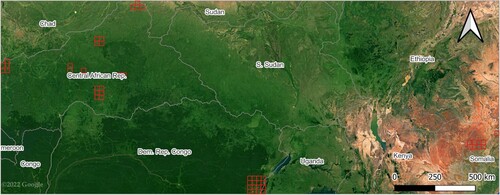
The ROI was determined by the availability of validation samples for the later stages of this work. It consists of 50 detached squared areas of approximately $750{\mathrm{km}}^2$ depicted by red polygonal shapes in Figure 1, spanning a total area of approximately $38,000{\mathrm{km}}^2$ across the Central African Republic, Somalia, the Democratic Republic of the Congo, and Uganda.

Figure 1. Region of interest.

3. Data

Various sources of data were used for various stages of this work. They are presented in the following subsections.

3.1. Datasets for extracting training samples

The training dataset was extracted from a new dataset built upon seven existing HRLC maps available in the ROI with a baseline year close to 2019. Six of those maps have a global extent, while one of them has a continental extent, thus they cover ROI completely. Regarding the typology of the existing HRLC maps, they can be divided into general and thematic LC maps. A map that encompasses all LC types in a landscape is referred to as a general LC map. Conversely, if a map depicts one or a few specific LC types, it is considered a thematic LC map. In the case of the latter, the map features a class representing a specific LC type, along with a class that encompasses all other LC types (e.g. Forest and Non-Forest categories). Three existing HRLC maps used in this work are general, and four are thematic maps depicting Built-up areas, Forest, or Water.

FROM-GLC consists of irregular time series of generic LC maps released by Tsinghua University (Gong et al. 2019, 2013; Li et al. 2017). The 2017 map at 10 m resolution was utilized in this work (Gong et al. 2019). Its legend consists of 10 classes: Cropland, Forest, Grass, Shrub, Wetland, Water, Tundra, Impervious, Bare land, and Snow/Ice. It is provided in ${10}^{\circ }\times {10}^{\circ }$ tiles in World Geodetic System 1984 (WGS84) Coordinate Reference System (CRS). The reported OA of this map is 73%.

The GL30 is regular time series of generic LC maps at 30 m resolution created by the National Geomatics Center of China (NGCC) (Chen et al. 2015). The GL30 legend comprises of 10 classes, including Cultivated land, Forest, Grassland, Shrubland, Wetland, Water bodies, Tundra, Artificial surfaces, Bare land, and Permanent snow and ice. The 2020 product was the input of this work. Its OA is 86%, as reported on GL30 official website. The product is distributed in Universal Transverse Mercator (UTM) projection. The tile size of GL30 is location-dependent. The major part of tiles (between ${60}^{\circ }\mathrm{N}$ and ${60}^{\circ }\mathrm{S}$) are $5^{\circ }\times 6^{\circ }$ size, but they can be $5^{\circ }\times {12}^{\circ }$ or larger.

The ESA Climate Change Initiative (CCI) LC team has created a 20 m resolution LC prototype for Africa, hereafter referred to as the CCI Africa Prototype (Santoro et al. 2017). This map represents the state of LC in Africa in the year 2016. It has 10 general classes: Trees cover areas, Shrubs cover areas, Grassland, Cropland, Vegetation aquatic or regularly flooded, Lichen and mosses/sparse vegetation, Bare areas, Built up areas, Snow and/or ice, and Open water. It can be accessed as a single GeoTiff file in WGS84 CRS covering the entire African continent. The accuracy of the CCI Africa Prototype was estimated in four countries: Kenya, Gabon, Ivory Coast, and South Africa (Lesiv et al. 2019). The results showed an OA of 44% for South Africa, 47% for Ivory Coast, 56% for Kenya, and 91% for Gabon.

The Global Human Settlement Built-up (GHS BU) is a collection of thematic maps that differentiate between built-up and non-built-up surfaces (Corbane et al. 2017; Pesaresi et al. 2016)produced by the Joint Research Center (JRC) of the European Commission. There are various GHS BU products that vary in terms of their input imagery, baseline year, and production method. The particular product used in this work, GHS BU S1NODSM, is based on Sentinel-1 imagery from 2016 and has two classes, Built-up and Non built-up. This product is distributed as a zip file of $2^{\circ }\times 2^{\circ }$ tiles covering the whole globe. The tiles have a Web Mercator projection (EPSG:3857) as its original Coordinate Reference System. The accuracy of GHS BU S1NODSM is only described qualitatively in comparison to another LC dataset (Corbane et al. 2017).

Another thematic LC product dedicated to built-up areas is WSF from German Aerospace Center – DLR (Marconcini et al. 2021, 2020). It features two classes, labeled as settlements and non-settlements. The product includes two maps with a spatial resolution of 10 m, one for 2015 and another for 2019. The later map was used in this work. The WSF is available in $2^{\circ }\times 2^{\circ }$ tiles in WGS84 CRS. The WSF for 2019 has $\mathrm{OA}=84\text{\%}$ and a $\mathrm{Kappa}=0.65$, but the information about UA, and PA are not available yet.

The GSW family is a collection of multi-temporal thematic LC maps that focus on several aspects of inland water bodies (Pekel et al. 2016). The thematic maps are annual maps for 36 years from 1984 to 2020. They are produced by JRC. The product offerings of GSW include monthly water history, seasonality, yearly history, water occurrence, change intensity, recurrence, transitions, maximum water extent, monthly recurrence, and metadata. For the purposes of this work, the yearly history for 2019 was used. Yearly history includes two water classes, seasonal and permanent, which were merged and treated as a single class – Water. The User's accuracy (UA) and Producer's accuracy (PA) of the whole time series, including 2019 map, is higher than 95%.

FNF is a thematic LC map that categorizes forested regions across the world (Shimada et al. 2014). Developed by the Japan Aerospace Exploration Agency (JAXA), it offers a multi-temporal representation of forest areas, with irregular time intervals. The map covers the time periods from 2007 to 2010 and from 2015 to 2020, and classifies areas as forest, water, and not water, with a resolution of approximately 25 m. FNF for 2019 was used in this work. The accuracy of this specific product is not reported. The product is distributed in two tile sizes: $1^{\circ }\times 1^{\circ }$ or $5^{\circ }\times 5^{\circ }$ from its official website.

3.2. Satellite imagery and auxiliary data for classification

Besides the training dataset, input data for classification were two types of satellite imagery – Sentinel-2 and Planet, and one DEM (Digital Elevation Model) dataset – CGIAR-CSI (Consultative Group on International Agricultural Research – Consortium for Spatial Information) SRTM (Shuttle Radar Topography Mission) DEM.

The Sentinel-2 mission is part of the Copernicus program and was developed by the European Space Agency (ESA) (ESA 2023). It consists of two satellites, Sentinel-2A and Sentinel-2B, which were launched into orbit in 2015 and 2017. These satellite platforms can capture high-resolution images, with a resolution of 10 m, and cover the entire globe every five days. The Sentinel-2 mission produces images in 13 different spectral bands, including 8 with 10 m resolution, 4 with 20 m resolution, and 1 with 60 m resolution. All the images produced by Sentinel-2 are freely accessible to the public.

Planet-NICFI Basemaps for Tropical Forest Monitoring is a product distributed through Norway's International Climate and Forest Initiative (NICFI) which gives access to Planet's high-resolution optical imagery over the tropical regions. The product incorporates the products from different Planet missions into analysis-ready mosaics distributed on a monthly and biannual basis, freely distributed for research and non-commercial use. The basemaps can be accessed directly through the Google Earth Engine (GEE) platform, offering orthorectified and mosaicked images with a spatial resolution of 4.77 m. The dataset consists of three visible bands and one near-infrared band, which can be utilized to identify LC and vegetation types.

The CGIAR-CSI SRTM DEM is a digital elevation model used to support classification. It is a product of the CGIAR-CSI, which is a revised version of the original SRTM of NASA (National Aeronautics and Space Administration) (Jarvis et al. 2008). The resolution of the product is 90 m at the equator. The revision process involved interpolation and the utilization of additional DEMs, with the goal of filling in any gaps in the original SRTM dataset. The CGIAR-CSI SRTM DEM is available for non-profit use at no cost.

4. Methodology

4.1. Conceptualization

Training data were extracted from a new dataset obtained by combining existing HRLCs described in Section 3.1. Existing HRLCs are combined by intersection so that only the areas that have unanimous agreement among them are retained (Figure 2). Any pixels that exhibit divergent values among the intersected HRLCs are considered non-agreement and are thus set to null. The resulting output dataset is named a Map of Land Cover Agreement (MOLCA).

Figure 2. Illustration of the derivation of the Map Of Land Cover Agreement – MOLCA.

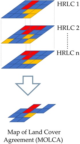
Theoretically speaking, the MOLCA is likely to have high accuracy because a consensus among multiple datasets increases the probability of accurate pixel classification. Correctly classified pixels are expected to be consistently present across various datasets due to the classification procedure's goal of accurate classification. Conversely, errors may occur due to various factors such as inadequate training data, unsuitable classification algorithms, imprecise satellite imagery, the complexity of land cover types, and atmospheric disturbances like cloud cover. Since existing HRLCs are created by different agencies and procedures, it is unlikely that errors in different datasets will be replicated across multiple datasets. MOLCA's accuracy evaluation shows an OA of 96% in ROI, with most classes having high UA and PA above 90%. This level of accuracy is significant, considering that even expert photo interpreters can make mistakes while labeling samples (Brown et al. 2022; Sun, Chen, and Zhou 2016).

In order to have an effective MOLCA derivation procedure, CRS, resolution and legend of the existing HRLCs had to be harmonized. These characteristics vary in existing HRLCs because of the lack of standard production procedures; however, if they are not harmonized, there is a risk that MOLCA production would not yield any result because the intersection procedure eliminates differences.

The baseline year of input existing HRLCs varied between 2016 and 2020, therefore this is the time frame of representativeness of MOLCA. This temporal variation is not an issue as any land cover change that might have occurred during the time between the oldest and most recent HRLC inputs is removed in the intersection, and therefore will not impact the quality of MOLCA.

4.2. MOLCA creation and training data extraction

The MOLCA derivation procedure was designed and developed in the ESA CCI HRLC project. The focus of the project was on three macro-regions of the world that are prone to stronger effects of climate change: Amazon, Siberia, and Sub-Saharan Africa. MOLCA was produced in all three macro-regions (Bratic and Brovelli 2023), but in this study, only the portions of it falling in the ROI were used.

The procedure of MOLCA derivation was based on GRASS GIS and Python (GRASS Development Team 2022; Python Software Foundation 2022). Python use was either independent of GRASS GIS, or was utilized to automatize GRASS GIS operations. The workflow of the procedure is depicted in Figure 3.

Figure 3. Overview of MOLCA production workflow.

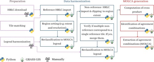
The MOLCA creation started with downloading existing HRLCs in regions of interest. This was performed with custom Python scripts, or manually when automatization was not possible. Tiles of each HRLC were stored in a subfolder of one main folder containing all existing data.

The legends of these input HRLCs were meticulously compared to determine the corresponding classes. The classes that consistently appeared across multiple datasets were designated as the target classes for MOLCA. Consequently, a correspondence table was established for each existing HRLC dataset, aligning their legends with the target legend of MOLCA. This process can be referred to as the harmonization of legends between existing HRLCs and the desired legend of MOLCA. The legend harmonization was done manually because the same class might have a different name and code in different HRLCs. Based on correspondence tables, txt files with reclassification rules were created to be used in later steps. The reclassification rules contain information about the original raster value and target raster value, and optionally target class label. The comprehensiveness of the legend of MOLCA was determined by the comprehensiveness of the input HRLC datasets. It contains Bareland, Built-up, Cropland, Forest, Grassland, Permanent ice and snow, Shrubland, Water, and Wetland classes.

A reference HRLC dataset was selected to serve as guidance for the CRS, extent, and spatial resolution of the MOLCA tile, but it was not used as an input dataset for MOLCA. Since MOLCA was generated in the CCI HRLC project, a tile of CCI HRLC product, which has a size of 100 km × 100 km, a resolution of 10 m, and WGS84 CRS was selected.

Different datasets come in different tiling systems. For this reason, it is necessary to find the matching tiles across the datasets. By using the os, rasterio, and geopandas libraries in Python, we created a script with an algorithm for matching tiles. The algorithm iterates through a folder with reference dataset tiles, extracts the extent of the tiles, and saves them in a vector along with the tile path information. Subsequently, it iterates through a folder with existing non-reference datasets, extracts the extent of the tiles, converts them into the reference CRS, and saves them in another vector, keeping information about the tile path. Finally, the two vectors are intersected. The resulting vector contains an attribute with the reference dataset path and an attribute with paths of spatially corresponding tiles of other non-reference HRLCs. The vector attributes were saved as a CSV file.

We also created an algorithm for MOLCA generation which performs harmonization of different characteristics of input HRLCs and for the extraction of their areas of agreement.

The choice of CRS upon creation of the GRASS GIS database determines the CRS to which all imported datasets will be reprojected. In this case, it was WGS84.

Based on the CSV file of matching tiles across different datasets, the MOLCA generation algorithm imports data for MOLCA creation. The algorithm first imports a tile of reference dataset and defines the GRASS GIS region according to it. The GRASS GIS region determines the extent and resolution at which the raster processing operations will be performed. The reference dataset is also reclassified to MOLCA legend. Then, all tiles of non-reference HRLCs that are available in the same location as the tile of the reference dataset are imported. In case some portions of non-reference tiles cross the extent, those portions were discarded on the import by using the appropriate flag. Some tiles of non-reference might be smaller than the reference dataset. Therefore, for each reference tile, the algorithm checks if a non-reference HRLC has more than one spatially corresponding tile. In the event of multiple tiles, they are imported and merged together. Subsequently, the tiles of non-reference existing HRLCs are reclassified to the MOLCA target legend.

At this point of the procedure, the datasets are harmonized with respect to CRS, extent, and legend. There is no need to resample them to the same resolution because this is done on the fly due to the GRASS GIS region definition. Next, the algorithm computes cross-product from non-reference datasets. The cross-product is a raster map that has different values for each distinct combination of class values found within the input raster layers. Cross-product also includes labels of classes included in the combinations. These cross-product labels are parsed and analyzed to identify agreement labels, characterized by having the same label for each input HRLC or the same label for at least two HRLCs, with other labels designated as NULL. The agreement labels and their associated values are subsequently converted into reclassification rules. Finally, the cross-product is reclassified into the MOLCA.

The total number of pixels in MOLCA within the ROI of this study was 82,650,430, which covers around 21% of ROI. A stratified random sampling strategy was employed to select 8000 training samples from each MOLCA class. The number of pixels of Bareland and Wetland classes was below 8000, therefore all available pixels of these two classes were selected. The number of Bareland samples was 22, and the number of Wetland samples was 6. Unfortunately, there were no pixels of Ice and snow (permanent) in MOLCA, so training samples of this class were not available for training RF, and consequently they were absent from the final classification, even though this class is present on the ground in ROI. In total, there were around 48,000 training samples extracted.

4.3. Classification

The advancement of technology and the availability of free and open remote sensing data has enabled the development of cloud tools and services for analyzing and mapping Earth's surface at a global scale. As such, in the current work was adopted and utilized GEE, a cloud-based platform that provides access to planetary-scale computation and a vast data catalog (Gorelick et al. 2017), to pre-process Sentinel-2 and Planet images and to apply Random Forest algorithm. One of the key advantages of GEE is its ability to access a vast amount of remote sensing data (historical and near-real time), including observations from missions like Landsat, Sentinel, and MODIS. The ability to perform large-scale, time-series geospatial analyzes makes it preferable in various research domains, e.g. land cover and crop mapping, deforestation, water and air quality monitoring, and, disaster domain (Brovelli, Sun, and Yordanov 2020; Hirschmugl et al. 2020; Yang et al. 2022; Yordanov and Brovelli 2021).

The GEE platform provides a range of algorithms and tools suitable for land cover classification, such as supervised and unsupervised classification, pixel- or object-based machine learning algorithms, and image analysis. Both collections used in this work, Sentinel-2 and Planet-NICFI, were accessible from the data catalog, only the latter is available upon free registration. In overview, three variations of the datasets as input were used Sentinel-2 allB (using all available bands); Sentinel-2 4B (using only the Red, Green, Blue, and Near-Infrared bands) and Planet 4B (the Red, Green, Blue, and Near-Infrared bands). The described below processing steps are similar to all datasets with small differences during the filtering stage for Planet 4B. In addition to the satellite imagery was used elevation information derived from CGIAR-CSI SRTM DEM, namely elevation and slope inclination. Additional feature datasets produced locally were used in GEE as imported assets, namely, regions of interest ROI (see Figure 1), training samples (Section 4.1), and validation point samples (Section 4.4).

A relatively standard processing workflow for image classification is usually subdivided into four main steps – import and filtering, preparation of the training information, model training, and model evaluation.

Import and filtering – at this stage all datasets were imported into the working environment. The Sentinel-2 and Planet collections were called image collections, while the additional data related to the ROI, training, and testing points as feature collections from the user's private asset storage. Both of the image collections were primarily filtered according to a time period of interest (01 January–31 December 2017) and ROI.

The period of interest was selected somewhat arbitrarily. The input training data represent the time period between 2016 and 2020. We chose a specific time frame for our study because the general HRLCs contribute the most to the creation of the classes in MOLCA that is a source of training data (i.e. thematic maps contribute just to one class at a time). Since the general maps are for 2016, 2017, and 2019, the year of the map in the middle was selected, but it could have been any year between 2016–2020.

A further pre-processing step was needed to remove the effect of cloud cover in the optical images, which particularly in the tropical region can significantly reduce the number of usable images. In the case of Sentinel-2 were performed two strategies – (1) the images were filtered to be containing less than 10% cloud cover according to the ‘cloudy pixel percentage’ property and (2) the left cloudy pixels were removed using the cloud bitmasks. On the other hand, in the case of Planet datasets such cloud filtering was not possible as the Planet images are, in fact, monthly mosaics, therefore, for them, it was only possible to filter by date and in a period of one year were available 12 images.

The DEM was also imported and using the ‘Terrain’ function container was computed also the slope.

Preparation of the training information – during this stage of processing the bands that will be used for the model were defined, i.e. three separate lists containing the band names were created according to each variation of the dataset (Sentinel-2 allB/4B and Planet 4B). In addition, all training and validation point datasets were used to sample the image collections using the ‘sample Regions’ function.

Model training – several machine learning models are available for use in the GEE environment (e.g. Random Forest, Support Vector Machine, etc.). The adopted approach in this work was to apply a supervised pixel-based classification. In particular, for the aim of land cover classification, it was chosen Random Forest algorithm (Breiman 2001) which is a type of ensemble learning algorithm that combines multiple decision trees to improve the accuracy and robustness of a model. It works by constructing a set of decision trees based on randomly sampled subsets of the training data. Each decision tree is built by recursively splitting the data into smaller subsets based on the features that provide the most information gain for the classification task. The splitting process continues until a stopping criterion is met, such as reaching a certain depth or achieving a minimum number of samples in each leaf node. Random Forest is a powerful machine learning algorithm which can handle both categorical and continuous datasets and is less prone to overfitting, which makes it preferable and widely adopted in many geospatial applications. In fact, it delivers reliable results and is one the most used machine learning models implemented in the GEE system (Yang et al. 2022).

Even though several models are available for the users, some other popular frameworks as scikit-learn, XGBoost, TensorFlow or PyTorch, cannot be directly used in GEE, and would require outside of the environment trainings. For the current application, the Random Forest classifier was used with a very straightforward parameterization using a forest of 100 decision trees which yielded a satisfactory compromise between accuracy and computational load.

Model evaluation – to evaluate the performance of the built model were used the implemented algorithms in GEE containers related to estimating the outputs' accuracies, namely, the error matrix computation from which was possible to compute the Overall Accuracy and Cohen's Kappa coefficient for each input and validation iteration. The details about the validation datasets are described in detail in the following Section 4.4.

4.4. Validation approach

One part of the validation dataset consisted of validation samples used for MOLCA validation. Following the logic of reference data collection by photo-interpretation, where the consensus of multiple annotators indicates classes that are easy to recognize and annotate (Brown et al. 2022), manyfold agreement of existing HRLCs based on which MOLCA is created indicate easy-to-classify areas. Since MOLCA is most likely to represent easy-to-classify areas, the same is true for the sample points used for its validation. For this reason, additional samples were added in hard-to-classify areas to have a more balanced validation dataset. Samples in easy-to-classify areas were selected following a stratified random sampling strategy. Stratification was done based on MOLCA classes, and therefore the size of each stratum was equal to the size of the corresponding MOLCA class. The total number of samples was estimated following the Equation (1(1) $n=\frac{p\ast q}{(\frac{E}{z_{\alpha }}{)}^2}$(1) ) (Cochran 1977) in which n is the number of sample plots, E is the acceptable margin of error for the sample, $z_{\alpha }$ is the z-value on the normal distribution corresponding to a certain level of confidence, p represents the expected accuracy, and q = 1−p. (1) $n=\frac{p\ast q}{(\frac{E}{z_{\alpha }}{)}^2}$(1)

The parameters inserted in the Equation (1(1) $n=\frac{p\ast q}{(\frac{E}{z_{\alpha }}{)}^2}$(1) ) are: p = 50%, E = 3%, and $z_{\alpha }=1.96$ (for the confidence interval of 95%).

The equation resulted in 1068 samples for validation. Some of these samples were rejected during photo-interpretation due to uncertainty. To make up for the eliminated samples, 130 additional samples were included. The distribution of samples among strata was equal. So, there were 195 samples per strata, except for Bareland and Wetland classes. As these two classes had fewer than 195 pixels in MOLCA, obtaining more samples was impossible. Consequently, the maximum number of samples for these two classes was determined by the maximum number of pixels in MOLCA, which was 22 for Bareland and 6 for Wetland. Random selection was used to choose samples in each stratum, except for Bareland and Wetland, where all of their pixels were used as samples.

The definition of hard-to-classify areas was done based on areas of discrepancy between GL30 and CCI Africa Prototype. The number of samples in hard-to-classify areas was determined in the same way as for easy-to-classify areas, but it was increased to 1085 to take into account a minimum of 3 samples per strata. Strata in the case of hard-to-classify areas were confusion types between GL30 and CCI Africa Prototype. The distribution of samples per stratum was done proportionally to the stratum size.

The selection of the location of both easy-to-classify and hard-to-classify samples was done in GRASS GIS, then a photo-interpretation survey design was prepared in Open Foris Collect (Open Foris Team 2021), and finally, the photo-interpretation was done with Collect Earth software (Bey et al. 2016). Photo-interpretation survey design integrates information about the location of the points, plot size, list of classes to be assigned to photo-interpreted samples, subjective confidence measure of photo-interpreter, photo-interpreter username, and date of photo-interpretation. The survey is imported into Collect Earth where it serves as a guide to label samples. Collect Earth provides Google Earth imagery and temporal profiles of vegetation indices from Landsat7/8, Sentinel-2, and MODIS imagery. Based on this information, a photo interpreter assigns class labels to the samples as well as the subjective level of confidence in photo interpretation. The size of the sample plot was $30\mathrm{m}\times 30\mathrm{m}$ to take into account the potential location error of VHR images.

Eventually, 1683 confident validation samples were obtained – 1050 in easy-to-classify areas, and 633 in hard-to-classify areas.

Accuracy was evaluated for all three classification outputs – Sentinel-2 4B, Sentinel-2 allB, and Planet 4B. The evaluation was done separately for areas that were easy-to-classify, areas that were hard-to-classify, and for a combination of both types of areas. The evaluation utilized standard accuracy metrics, such as OA, PA, and UA (Story and Congalton 1986), which were calculated from error matrices that were derived from validation samples and the classification outputs.

4.5. Comparison with existing land cover maps

To evaluate the success of MOLCA in the role of training samples, we compared the land cover product obtained from MOLCA (i.e. Sentinel-2 allB) with several land cover products obtained from samples collected with traditional approaches. The datasets which participated in MOLCA creation were not considered for the comparison because the results would be biased. The comparison was done with World Cover for 2020 (Van De Kerchove et al. 2021), Esri land cover for 2017 (Karra et al. 2021), and the Dynamic World for 2017 (Brown et al. 2022). This was done by estimating the accuracy of these three datasets with all validation samples collected for our study and comparing the results to the accuracy results of the Sentinel-2 allB. The accuracy estimations were done on GEE since all three datasets are directly accessible through it. To condense the extensive dataset comprising the classification results of each individual Sentinel-2 tile from the complete Sentinel-2 archive within the Dynamic World, a median value was calculated for tiles from year 2017 within the Region of Interest (ROI), thereby reducing it to a singular temporal dimension. The datasets were reclassified to the legend of the validation dataset, and then they were sampled in the location of validation points on GEE. In the case of the Esri land cover dataset, the Grassland and Shrubland classes are merged into a single class – Rangeland. For the comparison with this dataset, these two classes were merged into a single class for our land cover map too.

Finally, the error matrix was computed for each dataset by cross-tabulating classes of the existing HRLCs with classes of validation dataset. Subsequently, OA, PA, and UA were computed too.

5. Results and discussion

5.1. Validation results

The results of OA for three different classification tests with three different validation datasets are presented in Table 1. The study found that the accuracy was highest for the Sentinel-2 allB product, which suggests that including more bands in the classification improves the classifier's ability to distinguish among different classes. Additionally, when comparing the accuracy of two products based on the same number of bands (namely, Planet 4B and Sentinel-2 4B), it was found that the accuracy of Planet 4B was slightly higher. This could be due to the higher resolution of Planet imagery. The accuracy of Sentinel-2 4B and Planet 4B products was lower than the accuracy of Sentinel-2 allB. Therefore, the following more detailed accuracy results are focused on analyzing the results of Sentinel-2 allB.

Table 1. OA of land cover products with different validation datasets.

	Validation dataset
Classification test	All areas	Easy-to-classify	Hard-to-classify
Planet 4B	73%	88%	49%
Sentinel-2 4B	68%	84%	41%
Sentinel-2 allB	78%	93%	52%

A more detailed result of the validation of Sentinel-2 allB with all validation samples, easy-to-classify, and hard-to-classify samples are presented with standard error matrixes in Tables 2–4, respectively. In these tables, validation reference data is represented by columns, while classification is represented by rows.

Table 2. Accuracy of Sentinel-2 allB product with all samples.

	Bareland	Built-up	Cropland	Forest	Grassland	Ice and snow	Shrubland	Water	UA	PA	OA
Bareland										0%	78%
Built-up		213	7	2	14		6		88%	98%
Cropland		1	99	18	36		13		59%	60%
Forest		1	17	282	29	2	68		71%	88%
Grassland	2	2	37	13	190		66	1	61%	65%
Ice and snow										0%
Shrubland	1	1	5	2	25		311		90%	67%
Water			1	4			1	205	97%	100%

Table 3. Accuracy of Sentinel-2 allB product with hard-to-classify samples.

	Built-up	Cropland	Forest	Grassland	Ice and snow	Shrubland	Water	UA	PA	OA
Built-up	1	4	2	11		6		4%	100%	52%
Cropland		34	11	12		11		50%	38%
Forest		15	99	27	2	68		47%	76%
Grassland		31	13	52		60	1	33%	43%
Ice and snow									0%
Shrubland		5	1	18		123		84%	46%
Water		1	4			1	19	76%	95%

Table 4. Accuracy of Sentinel-2 allB product with easy-to-classify samples.

	Bareland	Built-up	Cropland	Forest	Grassland	Shrubland	Water	UA	PA	OA
Bareland									0%	93%
Built-up		212	3		3			97%	98%
Cropland		1	65	7	24	2		66%	86%
Forest		1	2	183	2			97%	96%
Grassland	2	2	6		138	6		90%	79%
Shrubland	1	1		1	7	188		95%	96%
Water							186	100%	100%

In the case of validation with all samples (Table 2), it is evident that the Water class had the highest accuracy with both UA and PA close to 100%. The Built-up class also had high accuracy with a PA of 98% and a UA of 88%. The Forest class had good accuracy with an 88% PA and a 71% UA, but there was some overestimation due to Shrubland contamination. The Shrubland class was moderately underestimated with a PA of 67%, likely due to commission errors with Forest and Grassland classes. However, the UA was not significantly affected, at 90%. The Cropland and Grassland classes had moderate accuracy with UA and PA ranging from 59 to 65%. Both classes were overestimated – Grassland on the damage of Shrubland predominately, and the Cropland class on the damage of Grassland. The omission error of both classes was related to confusion among each other. The Bareland and Ice and snow (permanent) classes had a PA of 0%, and it was not possible to calculate UA in the absence of at least one correctly classified pixel in the location of validation points of those classes. The Ice and snow (permanent) class was not present in the classification products at all because it was not present in the training dataset, while the number of Bareland training samples was limited.

When accuracy assessed in hard-to-classify areas is concerned (Table 3), the Water class has the highest accuracy, but it is not very high and seems to be overestimated by contaminating the Forest class. The Shrubland class appears to be significantly underestimated (e.g. $\mathrm{UA}=46\text{\%}$) due to the misclassification of Forest, Grassland, Cropland, and Built-up. On the other hand, the Built-up class is severely overestimated (e.g. $\mathrm{PA}=4\text{\%}$). The overestimation of Built-up comes at the expense of Grassland and Shrubland mostly. The PA of Built-up is 100%, which indicates absolute accuracy, but it is based on a single sample of this class that is not representative. The accuracy of Grassland and Cropland is low, as they are confused with each other and also with other classes such as Shrubland. There were two validation samples of Ice and snow (permanent), but this class is not present in the products, and hence its omission error is 100%. Lastly, there were no Bareland samples in areas that are difficult to classify, and no classified pixels of Bareland in the locations of samples, and therefore this class is not present in the error matrix.

The validation results for easy-to-classify areas (Table 4) show high accuracy of many individual classes, such as Water, Forest, Shrubland, and Built-up. The accuracy of Grassland is relatively good, with a UA of 90%. However, PA is somewhat lower, indicating an underestimation of this class, mainly due to the overestimation of Cropland. The accuracy of Cropland is good based on the PA (86%), while the UA is slightly low (66%) due to the commission error over Grassland.

The accuracy results show expected behavior – higher accuracy in easy-to-classify areas than in hard-to-classify areas. Grassland and Cropland are the most challenging classes to classify, even in easy-to-classify areas. Additionally, the error matrix indicates a high omission error for the Shrubland class in hard-to-classify areas, which is also observed in the error matrix for all areas. In hard-to-classify areas, the Built-up class appears to be severely overestimated. However, this discrepancy is likely due to the limited number of validation samples available for this class in hard-to-classify areas.

The land cover map that is the result of Sentinel-2 allB classification is shown in Figure 4. The upper part of the figure shows the land cover product for complete ROI, the left lower part shows a zoomed subset of the land cover map, and the right lower part represents Google Image for the zoomed area. The zoomed subset of ROI that is in the central-southern part of ROI on the border between the Democratic Republic of Congo and Uganda.

Figure 4. Land cover map obtained in Sentinel-2 allB classification test.

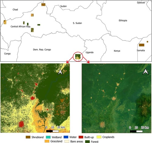
Visual inspection of the land cover map shows that it generally corresponds to what is visible in the basemap of Google imagery. For example, the forest, water, and built-up areas seem to be well detected. On the other hand, also some confusion between grassland and cropland is visible, which corresponds to the accuracy figures. In the zoomed area, a particularly critical region is displayed. Namely, in the southeast of the zoom area, there is Rwenzori mountain. It is critical for two reasons: it has high cloud coverage, and also it is the only area within ROI with Ice and snow (permanent) class. Reconstruction of cloudy images was not completely successful, and class Ice and snow (permanent) was not available in the training dataset so these two factors affected the outcome of the classification in the Rwenzori mountain area. It can be seen that there are rather large, unusually homogeneous patches of Shrubland, that are probably a consequence of cloud reconstruction. Also, there are many pixels of Built-up areas which are probably classified instead of Snow and ice and Bareland classes.

5.2. Comparison results

The accuracy of World Cover, Dynamic World and Esri land cover was estimated based on all validation samples collected for our study. The accuracy of these three datasets, together with the accuracy of Sentinel-2 allB product is reported in Table 5. It can be seen that the OA of Sentinel-2 allB is higher than the accuracy of other datasets. The existing HRLC with the highest OA among the ones included in the comparison is World Cover. The UA and PA of World Cover are not drastically different than the ones of Sentinel-2 allB. The major difference is the extremely low PA of the Cropland class in the case of World Cover. Similarly, the other two datasets have extremely low PA for the Cropland class, but also low UA for the Forest class compared to World Cover and Sentinel-2 allB.

Table 5. Comparison of the accuracy of World Cover, Dynamic World and Esri land cover with the accuracy of Sentinel-2 allB product.

	World Cover		Dynamic World		Esri land cover		Sentinel-2 allB
	PA	UA	PA	UA	PA	UA	PA	UA
Bareland	0%	0%	33%	6%	0%	0%		0%
Built-up	80%	98%	98%	88%	98%	93%	88%	98%
Cropland	6%	85%	9%	20%	4%	60%	59%	60%
Forest	94%	60%	95%	43%	95%	41%	71%	88%
Grassland	63%	56%	27%	72%	51%	80%	61%	65%
Shrubland	72%	75%	57%	81%			90%	67%
Water	98%	99%	93%	97%	100%	97%	97%	100%
Wetland	0%	0%
Ice and snow	50%	100%	100%	40%				0%
OA	72%		64%		67%		78%

6. Conclusions

This paper presents a way to extract the most reliable parts of the existing HRLC datasets that can serve as training data for creating a new HRLC map. The use case of land cover production in one ROI in Africa served as a base to describe the methodology and its effectiveness. The objective was to provide an innovative and reliable low-cost dataset to address the challenge of training reference data collection. The challenge is particularly emphasized in the case of global land cover production in which producers sometimes opt for lower reliability to reduce costs. However, the reliability of reference data is essential because it directly affects the quality of land cover products based on them.

The methodology proposes combining existing HRLCs by intersection. The outcome is a new dataset – MOLCA – that consists only of areas in which all existing HRLCs show consistent information about LC class. In the use case, MOLCA was a pool to extract around 8000 samples per class available in MOLCA. The samples were used to train the RF algorithm with Sentinel-2 or Planet NICFI imagery, and subsequently to produce the land cover. There were three land cover maps produced with three different classification tests – Sentinel-2 allB, Sentinel-2 4B, and Planet4B. The accuracy of all three land cover maps was estimated against three different sets of validation samples - easy-to-classify, hard-to-classify, and a combination of the previous two.

Different classification tests allowed observing that the accuracy of image classification improves as the number of bands or resolutions increases. However, the number of bands seems to be more important than the resolution. I.e. classification test of Sentinel-2 allB (12 bands at 10 m resolution) was better performing than Planet 4B (4 bands at 4.77 m resolution). This is probably because machine learning algorithms have more features to learn from when there are more bands involved in the classification. In any case, it is important to be aware that there are different factors affecting the accuracy, except the quality of training data.

Different validation exercises allowed a more detailed insight into accuracy. Some of the obtained results are expected, i.e. that the accuracy will be higher in the easy-to-classify areas than in hard-to-classify areas. On the other hand, it is curious to observe some extreme behavior such as the high accuracy of the Water class in hard-to-classify areas in which all the other classes show a low accuracy; or relatively low UA of Cropland and PA of Grassland in easy-to-classify areas.

To compare the HRLC dataset obtained in this study with existing HRLCs, the focus was on accuracy estimation of these datasets using a combination of easy-to-classify and hard-to-classify samples. This is because the combination of two types of samples provides a more balanced and accurate assessment of the classification performance. In the comparison of Sentinel-2 allB with World Cover, Dynamic World, and Esri land cover datasets it was shown that Sentinel-2 allB has the highest OA among these datasets – 78%. Since the validation dataset was prepared for validation of the classification results of this study, it can be considered that the OA of the World Cover dataset is relatively similar to the one of Sentinel-2 allB (72%), while the other two datasets have OA lower for 10% or more.

The existing HRLCs which were used for the comparison are produced from photo-interpreted training samples, which are considered more reliable than using existing LC as a reference, but the procedure of obtaining them is laborious. On the opposite, MOLCA is based on existing LC, and it gives similar or better results at a significantly lower cost because less time and personnel are needed to obtain a big amount of samples (e.g. millions in this use case). Therefore, MOLCA qualifies as a suitable source of training samples for global land cover production. In fact, it could be particularly valuable for deep learning algorithms that require a substantial amount of training samples (Scott et al. 2017).

One limitation of the MOLCA approach is that it can fail to provide pixels of some classes that are present in the landscape. In this study, class Ice and snow (permanent) was missing, and it affected accuracy because those areas were classified as Built-up, as a consequence. Similarly, the number of samples was very small for Bareland and Wetland classes. This problem seems to be typical for the classes with small proportions in the landscape. Nevertheless, this drawback could potentially be solved by adapting the current methodology. One setback of the current methodology is that it does not check if all input HRLCs contain all target classes. If an input HRLC does not contain a particular class, then the MOLCA procedure will automatically eliminate that class due to the intersection procedure. The methodology could be adapted to integrate this step of verification if all input data contain all the classes, and if that is not the case, to exclude the dataset that misses one target class only when the creation of pixels of that class is concerned. An additional adaptation could be to introduce a voting schema for classes with small proportions, so that if the majority of input datasets agree on that class, MOLCA takes that value. However, in this case, it is necessary to take care that the reduction of rigidity does not cause the reduction of reliability.

Another way to address this limitation, if the adaption of methodology does not solve it, is to use a photo-interpretation to get the samples of missing classes. This would increase the costs compared to using only MOLCA samples, however, it would be still less expensive than providing all samples of all classes by photo-interpretation.

Future work will be focused on including existing HRLCs that are currently not involved in MOLCA production. Hopefully, this will further refine MOLCA, and help to address current limitations.

Disclosure statement

No potential conflict of interest was reported by the author(s).

Data availability statement

The datasets that support this study are freely available land cover datasets such as: FROM-GLC (http://data.ess.tsinghua.edu.cn/fromglc2017v1.html), GL30 (http://www.globallandcover.com/), CCI Africa Prototype (https://2016africalandcover20m.esrin.esa.int/), GHS BU S1NODSM (http://cidportal.jrc.ec.europa.eu/ftp/jrc-opendata/GHSL/GHS_BUILT_S1NODSM_GLOBE_R2018A/), WSF (https://download.geoservice.dlr.de/WSF2019/files/), GSW (https://global-surface-water.appspot.com/download), and FNF (https://www.eorc.jaxa.jp/ALOS/en/palsar_fnf/data/index.htm). GL30 and FNF require registration in order to retrieve the data, while CCI Africa Prototype require acceptance of terms of use. Satellite imagery, Planet NICFI Basemap (https://developers.google.com/earth-engine/datasets/catalog/projects_planet-nicfi_assets_basemaps_africa?hl=en) and Sentinel-2 (https://developers.google.com/earth-engine/datasets/catalog/COPERNICUS_S2), as well as CGIAR-CSI SRTM DEM (https://developers.google.com/earth-engine/datasets/catalog/CGIAR_SRTM90_V4), World Cover (https://developers.google.com/earth-engine/datasets/catalog/ESA_WorldCover_v100), Dynamic World (https://developers.google.com/earth-engine/datasets/catalog/GOOGLE_DYNAMICWORLD_V1) were obtained from Earth Engine Data Catalog. Esri land cover is directly accessible on Google Earth Engine through ‘awesome-gee-community-catalog’ by using ID projects/sat-io/open-datasets/landcover/ESRI$\mathrm{\_}$Global-LULC$\mathrm{\_}$10m$\mathrm{\_}$TS. ‘awesome-gee-community-catalog’ is a collection of geospatial datasets contributed by the community. MOLCA, which is the first dataset obtained by the methodology reported in this paper, is freely and openly available at https://doi.org/10.5281/zenodo.8071675.

Additional information

Funding

This research was partially supported by the European Space Agency (ESA) within the project CCI+ HRLC – Climate Change Initiative Extension (CCI+), Phase 1: New Essential Climate Variables (NEW ECVS) High Resolution Land Cover ECV (HR$\mathrm{\_}$LandCover$\mathrm{\_}$cci)(https://climate.esa.int/en/projects/high-resolution-land-cover).

References

- Abe, Camila, Felipe Lobo, Yonas Dibike, Maycira Costa, Vanessa Dos Santos, and Evlyn Novo. 2018. “Modelling the Effects of Historical and Future Land Cover Changes on the Hydrology of An Amazonian Basin.” Water 10 (7): 932. https://doi.org/10.3390/w10070932.
- Belward, Alan S., and Jon O. Skøien. 2015. “Who Launched What, When and Why; Trends in Global Land-Cover Observation Capacity From Civilian Earth Observation Satellites.” ISPRS Journal of Photogrammetry and Remote Sensing 103:115–128. https://doi.org/10.1016/j.isprsjprs.2014.03.009.
- Bey, Adia, Alfonso Sánchez-Paus Díaz, Danae Maniatis, Giulio Marchi, Danilo Mollicone, Stefano Ricci, Jean-François Bastin, et al. 2016. “Collect Earth: Land Use and Land Cover Assessment Through Augmented Visual Interpretation.” Remote Sensing 8 (10): 807. Accessed December 13, 2022. https://doi.org/10.3390/rs8100807.
- Birhanu, A., I. Masih, P. van der Zaag, J. Nyssen, and X. Cai. 2019. “Impacts of Land Use and Land Cover Changes on Hydrology of the Gumara Catchment, Ethiopia.” Physics and Chemistry of the Earth, Parts A/B/C 112:165–174. https://doi.org/10.1016/j.pce.2019.01.006.
- Bratic, Gorica, and Maria Antonia Brovelli. 2023. “Map of Land Cover Agreement – MOLCA.” Accessed June 30, 2023. https://doi.org/10.5281/ZENODO.8071675.
- Breiman, Leo. 2001. “Random Forests.” Machine Learning 45 (1): 5–32. https://doi.org/10.1023/A:1010933404324.
- Brovelli, Maria Antonia, Yaru Sun, and Vasil Yordanov. 2020. “Monitoring Forest Change in the Amazon Using Multi-Temporal Remote Sensing Data and Machine Learning Classification on Google Earth Engine.” ISPRS International Journal of Geo-Information 9 (10): 580. https://doi.org/10.3390/ijgi9100580.
- Brown, Christopher F., Steven P. Brumby, Brookie Guzder-Williams, Tanya Birch, Samantha Brooks Hyde, Joseph Mazzariello, Wanda Czerwinski, et al. 2022. “Dynamic World, Near Real-Time Global 10 M Land Use Land Cover Mapping.” Scientific Data 9 (1): 251. https://doi.org/10.1038/s41597-022-01307-4.
- Bunting, Pete, Ake Rosenqvist, Lammert Hilarides, Richard M. Lucas, and Nathan Thomas. 2022. “Global Mangrove Watch: Updated 2010 Mangrove Forest Extent (V2.5).” Remote Sensing 14 (4): 1034. https://doi.org/10.3390/rs14041034.
- Chen, Jun, Jin Chen, Anping Liao, Xin Cao, Lijun Chen, Xuehong Chen, Chaoying He, et al. 2015. “Global Land Cover Mapping At 30m Resolution: A POK-Based Operational Approach.” ISPRS Journal of Photogrammetry and Remote Sensing 103:7–27. https://doi.org/10.1016/j.isprsjprs.2014.09.002.
- Cochran, William G. 1977. Sampling Techniques. 3rd ed. Wiley Series in Probability and Mathematical Statistics, New York, NY: Wiley.
- Copernicus Open Access Hub. 2023. “Legal Notice on the Use of Copernicus Sentinel Data and Service Information.” Accessed March 29, 2023. https://sentinels.copernicus.eu/documents/247904/690755/Sentinel_Data_Legal_Notice.
- Corbane, Christina, Martino Pesaresi, Panagiotis Politis, Vasileios Syrris, Aneta J. Florczyk, Pierre Soille, Luca Maffenini, et al. 2017. “Big Earth Data Analytics on Sentinel-1 and Landsat Imagery in Support to Global Human Settlements Mapping.” Big Earth Data 1 (1-2): 118–144. https://doi.org/10.1080/20964471.2017.1397899.
- Cui, Guishan, Woo-Kyun Lee, Doo-Ahn Kwak, Sungho Choi, Taejin Park, and Jongyeol Lee. 2011. “Desertification Monitoring by Landsat TM Satellite Imagery.” Forest Science and Technology 7 (3): 110–116. https://doi.org/10.1080/21580103.2011.594607.
- Enoguanbhor, Evidence, Florian Gollnow, Jonas Nielsen, Tobia Lakes, and Blake Walker. 2019. “Land Cover Change in the Abuja City-Region, Nigeria: Integrating GIS and Remotely Sensed Data to Support Land Use Planning.” Sustainability 11 (5): 1313. https://doi.org/10.3390/su11051313.
- ESA. 2023. “Sentinel-2 MSI – Technical Guide – Sentinel Online – Sentinel Online.” Accessed March 29, 2023. https://sentinels.copernicus.eu/web/sentinel/technical-guides/sentinel-2-msi.
- Esch, Thomas, Felix Bachofer, Wieke Heldens, Andreas Hirner, Mattia Marconcini, Daniela Palacios-Lopez, Achim Roth, et al. 2018. “Where We Live–A Summary of the Achievements and Planned Evolution of the Global Urban Footprint.” Remote Sensing 10 (6): 895. https://doi.org/10.3390/rs10060895.
- Fritz, Steffen, Linda See, Christoph Perger, Ian McCallum, Christian Schill, Dmitry Schepaschenko, Martina Duerauer, et al. 2017. “A Global Dataset of Crowdsourced Land Cover and Land Use Reference Data.” Scientific Data 4 (1): 170075. https://doi.org/10.1038/sdata.2017.75.
- García-Álvarez, David, María Teresa Camacho Olmedo, Martin Paegelow, and Jean-François Mas. 2022. Land Use Cover Datasets and Validation Tools: Validation Practices with QGIS. Springer. https://doi.org/10.1007/978-3-030-90998-7.
- GCOS. 2021. The Status of the Global Climate Observing System 2021: The GCOS Status Report. Technical Report GCOS-240. Geneva: pub WMO. Accessed February 13, 2023. https://library.wmo.int/doc_num.php?explnum_id=10784.
- Giri, C., E. Ochieng, L. L. Tieszen, Z. Zhu, A. Singh, T. Loveland, J. Masek, and N. Duke. 2011. “Status and Distribution of Mangrove Forests of the World Using Earth Observation Satellite Data: Status and Distributions of Global Mangroves.” Global Ecology and Biogeography 20 (1): 154–159. https://doi.org/10.1111/j.1466-8238.2010.00584.x.
- Gong, Peng, Han Liu, Meinan Zhang, Congcong Li, Jie Wang, Huabing Huang, Nicholas Clinton, et al. 2019. “Stable Classification with Limited Sample: Transferring a 30-m Resolution Sample Set Collected in 2015 to Mapping 10-m Resolution Global Land Cover in 2017.” Science Bulletin 64 (6): 370–373. https://doi.org/10.1016/j.scib.2019.03.002.
- Gong, Peng, Jie Wang, Le Yu, Yongchao Zhao, Yuanyuan Zhao, Lu Liang, Zhenguo Niu, et al. 2013. “Finer Resolution Observation and Monitoring of Global Land Cover: First Mapping Results with Landsat TM and ETM+ Data.” International Journal of Remote Sensing 34 (7): 2607–2654. https://doi.org/10.1080/01431161.2012.748992.
- Gorelick, Noel, Matt Hancher, Mike Dixon, Simon Ilyushchenko, David Thau, and Rebecca Moore. 2017. “Google Earth Engine: Planetary-Scale Geospatial Analysis for Everyone.” Remote Sensing of Environment 202:18–27. https://doi.org/10.1016/j.rse.2017.06.031.
- GRASS Development Team. 2022. “Geographic Resources Analysis Support System (GRASS GIS) Software.” V. 8.2. Open Source Geospatial Foundation. http://grass.osgeo.org.
- Haddad, Nick M., Lars A. Brudvig, Jean Clobert, Kendi F. Davies, Andrew Gonzalez, Robert D. Holt, Thomas E. Lovejoy, et al. 2015. “Habitat Fragmentation and Its Lasting Impact on Earth's Ecosystems.” Science Advances 1 (2): e1500052. https://doi.org/10.1126/sciadv.1500052.
- Hansen, M. C., P. V. Potapov, R. Moore, M. Hancher, S. A. Turubanova, A. Tyukavina, D. Thau, et al. 2013. “High-Resolution Global Maps of 21st-century Forest Cover Change.” Science 342 (6160): 850–853. https://doi.org/10.1126/science.1244693.
- Hermosilla, Txomin, Michael A. Wulder, Joanne C. White, and Nicholas C. Coops. 2022. “Land Cover Classification in An Era of Big and Open Data: Optimizing Localized Implementation and Training Data Selection to Improve Mapping Outcomes.” Remote Sensing of Environment 268:112780. https://doi.org/10.1016/j.rse.2021.112780.
- Hirschmugl, Manuela, Janik Deutscher, Carina Sobe, Alexandre Bouvet, Stéphane Mermoz, and Mathias Schardt. 2020. “Use of SAR and Optical Time Series for Tropical Forest Disturbance Mapping.” Remote Sensing 12 (4): 727. https://doi.org/10.3390/rs12040727.
- Jarvis, Andy, Edward Guevara, Hannes Isaak Reuter, and Andy Nelson. 2008. “Hole-filled SRTM for the Globe Version 4.” Accessed December 30, 2022. https://srtm.csi.cgiar.org/.
- Karra, Krishna, Caitlin Kontgis, Zoe Statman-Weil, Joseph C. Mazzariello, Mark Mathis, and Steven P. Brumby. 2021, July. “Global Land Use / Land Cover with Sentinel 2 and Deep Learning.” In 2021 IEEE International Geoscience and Remote Sensing Symposium IGARSS, 4704–4707. Brussels, Belgium: IEEE. https://doi.org/10.1109/IGARSS47720.2021.9553499.
- Lesiv, M., L. See, B. Mora, S. Pietsch, S. Fritz, H. Bun, S. Sendabo, et al. 2019. “Accuracy Assessment of the ESA CCI 20m Land Cover Map: Kenya, Gabon, Ivory Coast and South Africa.” Accessed October 25, 2022. https://pure.iiasa.ac.at/id/eprint/16107/1/WP-19-009.pdf.
- Li, Congcong, Peng Gong, Jie Wang, Zhiliang Zhu, Gregory S. Biging, Cui Yuan, Tengyun Hu, et al. 2017. “The First All-Season Sample Set for Mapping Global Land Cover with Landsat-8 Data.” Science Bulletin 62 (7): 508–515. https://doi.org/10.1016/j.scib.2017.03.011.
- Lu, Zhiwu, Zhenyong Fu, Tao Xiang, Peng Han, Liwei Wang, and Xin Gao. 2017. “Learning From Weak and Noisy Labels for Semantic Segmentation.” IEEE Transactions on Pattern Analysis and Machine Intelligence 39 (3): 486–500. Accessed 2023-07-20. http://ieeexplore.ieee.org/document/7450177/. https://doi.org/10.1109/TPAMI.2016.2552172.
- Marconcini, Mattia, Annekatrin Metz-Marconcini, Soner Üreyen, Daniela Palacios-Lopez, Wiebke Hanke, Felix Bachofer, Julian Zeidler, et al. 2020. “Outlining Where Humans Live, the World Settlement Footprint 2015.” Scientific Data 7 (1): 242. https://doi.org/10.1038/s41597-020-00580-5.
- Marconcini, Mattia, Annekatrin Metz Marconcini, Thomas Esch, and Noel Gorelick. 2021. “Understanding Current Trends in Global Urbanisation – The World Settlement Footprint Suite.” GI_Forum 2021 9:33–38. https://doi.org/10.1553/giscience2021_01_s33.
- Morán-Fernández, Laura, Verónica Bólon-Canedo, and Amparo Alonso-Betanzos. 2022. “How Important Is Data Quality? Best Classifiers Vs Best Features.” Neurocomputing 470:365–375. https://doi.org/10.1016/j.neucom.2021.05.107.
- Open Foris Team. 2021. “Open Foris Collect.” Accessed December 10, 2022. https://www.openforis.org/.
- Pekel, Jean-François, Andrew Cottam, Noel Gorelick, and Alan S. Belward. 2016. “High-resolution Mapping of Global Surface Water and Its Long-Term Changes.” Nature 540 (7633): 418–422. https://doi.org/10.1038/nature20584.
- Pesaresi, Martino, Daniele Ehrlich, Stefano Ferri, Aneta Florczyk, Sergio Manuel Carneiro Freire, Stamatia Halkia, Andreea Maria Julea, et al. 2016. Operating Procedure for the Production of the Global Human Settlement Layer from Landsat Data of the Epochs 1975, 1990, 2000, and 2014. Technical Report EUR 27741. Joint Research Centre. Accessed July 12, 2020. https://ec.europa.eu/jrc/en/publication/operating-procedure-production-global-human-settlement-layer-landsat-data-epochs-1975-1990-2000-and.
- Picoli, Michelle Cristina Araujo, Gilberto Camara, Ieda Sanches, Rolf Simões, Alexandre Carvalho, Adeline Maciel, Alexandre Coutinho, et al. 2018. “Big Earth Observation Time Series Analysis for Monitoring Brazilian Agriculture.” ISPRS Journal of Photogrammetry and Remote Sensing145:328–339. https://doi.org/10.1016/j.isprsjprs.2018.08.007.
- Potapov, Peter, Svetlana Turubanova, Matthew C. Hansen, Alexandra Tyukavina, Viviana Zalles, Ahmad Khan, Xiao-Peng Song, et al. 2022. “Global Maps of Cropland Extent and Change Show Accelerated Cropland Expansion in the Twenty-First Century.” Nature Food 3 (1): 19–28. https://doi.org/10.1038/s43016-021-00429-z.
- Python Software Foundation. 2022. “Python V. 3.10.” https://www.python.org/.
- Radoux, Julien, Céline Lamarche, Eric Van Bogaert, Sophie Bontemps, Carsten Brockmann, and Pierre Defourny. 2014. “Automated Training Sample Extraction for Global Land Cover Mapping.” Remote Sensing 6 (5): 3965–3987. https://doi.org/10.3390/rs6053965.
- Santoro, M., G. Kirches, J. Wevers, M. Boettcher, C. Brockmann, C. Lamarche, and P. Defourny. 2017. “Land Cover CCI: Product User Guide Version 1.1.” https://climate.esa.int/media/documents/ESACCI-LC-Ph2-PUGv3_1.1.pdf.
- Schiavina, M., M. Melchiorri, M. Pesaresi, P. Politis, S. M. Carneiro Freire, L. Maffenini, P. Florio, et al. 2022. GHSL Data Package 2022. Technical Report KJ-07-22-357-EN-N (online), KJ-07-22-357-EN-C (print). Joint Research Centre (European Commission). https://doi.org/10.2760/19817.
- Scott, Grant J., Matthew R. England, William A. Starms, Richard A. Marcum, and Curt H. Davis. 2017. “Training Deep Convolutional Neural Networks for Land–Cover Classification of High-Resolution Imagery.” IEEE Geoscience and Remote Sensing Letters 14 (4): 549–553. Accessed 2023-02-28. https://doi.org/10.1109/LGRS.2017.2657778.
- See, Linda, Juan Carlos Laso Bayas, Myroslava Lesiv, Dmitry Schepaschenko, Olga Danylo, Ian McCallum, Martina Dürauer, et al. 2022. “Lessons Learned in Developing Reference Data Sets with the Contribution of Citizens: The Geo-Wiki Experience.” Environmental Research Letters 17 (6): 065003. https://doi.org/10.1088/1748-9326/ac6ad7.
- Shimada, Masanobu, Takuya Itoh, Takeshi Motooka, Manabu Watanabe, Tomohiro Shiraishi, Rajesh Thapa, and Richard Lucas. 2014. “New Global Forest/Non-Forest Maps From ALOS PALSAR Data (2007–2010).” Remote Sensing of Environment 155:13–31. https://doi.org/10.1016/j.rse.2014.04.014.
- Story, Michael, and Russell G. Congalton. 1986. “Accuracy Assessment: A User's Perspective.” Photogrammetric Engineering and Remote Sensing 52 (3): 397–399. https://www.asprs.org/wp-content/uploads/pers/1986journal/mar/1986_mar_397-399.pdf.
- Sun, Bo, Xi Chen, and Qiming Zhou. 2016. “Uncertainty Assessment of GlobeLand30 Land Cover Data Set Over Central Asia.” International Archives of the Photogrammetry, Remote Sensing and Spatial Information Sciences XLI-B8:1313–1317. https://doi.org/10.5194/isprsarchives-XLI-B8-1313-2016.
- Tarko, Agnieszka, Nandin-Erdene Tsendbazar, Sytze de Bruin, and Arnold K. Bregt. 2021. “Producing Consistent Visually Interpreted Land Cover Reference Data: Learning From Feedback.” International Journal of Digital Earth 14 (1): 52–70. https://doi.org/10.1080/17538947.2020.1729878.
- Van De Kerchove, Ruben, Daniele Zanaga, Wanda De Keersmaecker, Linlin Li, Nandika Tsendbazar, Myroslava Lesiv, and Olivier Arino. 2021. “World Cover: Product User Manual.” https://esa-worldcover.s3.amazonaws.com/v100/2020/docs/WorldCover_PUM_V1.0.pdf.
- Wang, Sherrie, William Chen, Sang Michael Xie, George Azzari, and David B. Lobell. 2020. “Weakly Supervised Deep Learning for Segmentation of Remote Sensing Imagery.” Remote Sensing 12 (2): 207. Accessed 2023-07-20. https://www.mdpi.com/2072-4292/12/2/207. https://doi.org/10.3390/rs12020207.
- Woodcock, Curtis E., Richard Allen, Martha Anderson, Alan Belward, Robert Bindschadler, Warren Cohen, Feng Gao, et al. 2008. “Free Access to Landsat Imagery.” Science 320 (5879): 1011–1011. https://doi.org/10.1126/science.320.5879.1011a.
- Yang, Liping, Joshua Driscol, Sarigai Sarigai, Qiusheng Wu, Haifei Chen, and Christopher D. Lippitt. 2022. “Google Earth Engine and Artificial Intelligence (AI): A Comprehensive Review.” Remote Sensing14 (14): 3253. https://doi.org/10.3390/rs14143253.
- Yordanov, V., and M. A. Brovelli. 2021. “Deforestation Mapping Using Sentinel-1 and Object-Based Random Forest Classification on Google Earth Engine.” The International Archives of the Photogrammetry, Remote Sensing and Spatial Information Sciences XLIII-B3-2021:865–872. https://doi.org/10.5194/isprs-archives-XLIII-B3-2021-865-2021.
- Zeng, Xiaopeng, Tengfei Wang, Zhe Dong, Xiangrong Zhang, and Yanfeng Gu. 2023. “Superpixel Consistency Saliency Map Generation for Weakly Supervised Semantic Segmentation of Remote Sensing Images.” IEEE Transactions on Geoscience and Remote Sensing 61:1–16. Accessed 2023-07-20. https://ieeexplore.ieee.org/document/10097682/. https://doi.org/10.1109/TGRS.2023.3300317.
- Zhang, Xiao, Liangyun Liu, Xidong Chen, Yuan Gao, Shuai Xie, and Jun Mi. 2021. “GLC_FCS30: Global Land-Cover Product with Fine Classification System At 30 M Using Time-Series Landsat Imagery.” Earth System Science Data 13 (6): 2753–2776. https://doi.org/10.5194/essd-13-2753-2021.
- Zhou, Qiang, Heather Tollerud, Christopher Barber, Kelcy Smith, and Daniel Zelenak. 2020. “Training Data Selection for Annual Land Cover Classification for the Land Change Monitoring, Assessment, and Projection (LCMAP) Initiative.” Remote Sensing 12 (4): 699. https://doi.org/10.3390/rs12040699.
- Zhu, Zhe, Michael A. Wulder, David P. Roy, Curtis E. Woodcock, Matthew C. Hansen, Volker C. Radeloff, Sean P. Healey, et al. 2019. “Benefits of the Free and Open Landsat Data Policy.” Remote Sensing of Environment 224:382–385. https://doi.org/10.1016/j.rse.2019.02.016.