Integrating OpenStreetMap tags for efficient LiDAR point cloud classification using graph neural networks

ABSTRACT

The urban environment exhibits significant vertical variations, Light Detection and Ranging (LiDAR) point cloud classification can provide insights for the 3D morphology of the urban environment. Introducing the adjacency relationships between urban objects can enhance the accuracy of LiDAR point cloud classification. Graph Neural Network (GNN) is a popular architecture to infer the labels of urban objects by utilizing adjacency relationships. However, existing methods ignored the power of the known labels of urban objects, such as crowd-sourced tagged labels from OpenStreetMap (OSM) data, in the inferring process. Therefore, this study proposes a strategy introduces OSM data into GNN for LiDAR point cloud classification. First, we perform an over-segmentation of the LiDAR point cloud to obtain superpoints, which act as basic elements for constructing superpoint adjacency graphs. Second, PointNet is applied to embed superpoint features and edge features are generated using these superpoint features. Finally, OSM data is associated with some part of superpoints and incorporated into the GNN to update the embedded features of superpoints. The results demonstrate that the GNN with OSM data significantly improves the classification accuracy of original GNN. The improvement highlights taking advantage of crowd-sourced geoinformation in LiDAR point cloud classification for understanding 3D urban landscape.

KEYWORDS:

• LiDAR point cloud classification
• OpenStreetMap data
• Graph neural networks
• Multi-modal data integration
• Prior knowledge

1. Introduction

The ‘World Urbanization Outlook’ from the United Nations predicts that 68% of the global population will live in urban areas by 2050. Therefore, sustainable development of the urban environment is crucial for human well-being, and land cover data is essential for studying and managing urban areas (Lei et al. 2021; Wang et al. 2022; Zhao et al. 2022). However, the geo-objects in urban areas are diverse and heterogeneous, with significant differences in height. The existing urban land cover data are two-dimensional, obtained primarily from optical remote sensing data, which are not suitable for characterizing the three-dimensional (3D) morphological structure of urban geo-objects (Khanal et al. 2020; Sklyar and Rees 2022). This problem limits research on local ecological environments (Solórzano et al. 2021; Wang et al. 2022).

Three-dimensional (3D) classification of urban land cover can be regarded as the classification of the point cloud that represents 3D urban geo-objects. Currently, this is primarily the classification of Light Detection and Ranging (LiDAR) point clouds. Classification of LiDAR point clouds can be divided into point-oriented methods and object-oriented methods. Point-oriented methods use supervised classifiers and point features to individually classify each point in the LiDAR point cloud (He et al. 2021), while object-oriented methods classify objects divided by point clouds, assigning all points in the object to the same category as the object. The object-oriented methods can use more features, such as object size and shape, to obtain smoother results. However, they are negatively affected by over-segmentation or under-segmentation of unsupervised methods. The point-oriented methods directly classify the point clouds point by point. Thus, they are not affected by the segmentation method, but their results often include some errors like salt-and-pepper noise (Guo et al. 2021).

Deep learning has emerged as an effective solution to the aforementioned problems, greatly improving the accuracy of point cloud classification. Point cloud data, being irregular and invariant to disorder and displacement, has led scholars to design various classification methods from different perspectives. Qi, Su, et al. (2017) and Qi, Yi, et al. (2017) proposed PointNet and PointNet++, which leverage perceptron and feature pooling to obtain local features of point clouds through encoding and decoding, optimizing point cloud classification. Jiang et al. (2018) introduced PointSIFT, a module that can be integrated into PointNet and adapts shape and scale to obtain directional information, which is then encoded and processed. PointASNL proposed by Yan et al. (2020) effectively eliminates noise from the original point cloud through adaptive weighting of the initial sampling points in PointNet’s ‘farthest point sampling’. Wang et al. (2020) utilized SoftpoolNet to obtain the feature matrix by aggregating features through a ‘soft pooling’ method. As input point clouds increase, computational difficulty increases, but Lang, Asaf, and Shai (2020) addressed this with SampleNet, a method that pre-samples the main input point clouds to improve subsequent computational efficiency. In addition, Convolutional Neural Networks (CNN) have been indirectly used in point cloud classification, leading to many innovations such as MCCNN (Liu et al. 2018), FPConv (Lin et al. 2020), ConvPoint (Boulch 2020).

In point-oriented methods, it is difficult to consider the interaction between geo-objects, which are generally expressed by graphical models. Although one such expression method, Conditional Random Field (CRF), can be used in postprocessing, its unary term calculation obtained by the classifier is independent of CRF. Furthermore, the development of a Graph Neural Network (GNN) incorporates reasoning into deep learning and enables end-to-end training (Li, Liu, and Pfeifer 2019). In GNNs, reasoning is obtained by transmitting the edge information of the graph, such as the CRF (Landrieu and Simonovsky 2018). Chen et al. (2018) have incorporated the knowledge graph into the graph network to define a framework for spatial and semantic reasoning. While traditional networks spend a lot of time on farthest point sampling and proximity query when processing point clouds, Grid-GCN (Xu et al. 2020) voxelizes the entire point cloud, providing information covering the entire cloud using the perceptual grid query (Coverage-Aware Grid Query, CAGQ). This is followed by the graph convolution module Grid Context Aggregation (GCA), which integrates contextual features and coverage information into the computation, providing faster learning speeds and more complete point cloud coverage. Meanwhile, based on the rotation invariance of point clouds, Zhou et al. (2021) proposed the positional adaptive graph convolution AdaptConv, which can adaptively adjust point cloud features based on dynamically learned features, improving the flexibility of graph convolution and effectively capturing various relationships of point clouds from different semantic parts. Recently, researchers have applied attention mechanisms to point cloud analysis tasks to focus on the important information of point clouds, thus making their features more useful (Wang et al. 2019; Xue et al. 2019).

Although GNNs have demonstrated a strong ability to consider interactions between geographic objects, this ability is underutilized in lidar point cloud classification for mapping 3D urban land cover. Specifically, OpenStreetMap (OSM), a crowd-sourced database updated and maintained by a community of volunteers, provides many geo-objects tagged with labels (e.g. building, road) (Elhousni, Zhang, and Huang 2022; Zhou et al. 2022; Fonte et al. 2019). These geo-objects and their labels can be used as prior knowledge in GNNs to infer the labels of other geo-objects that need to be identified in lidar point cloud classification. However, existing studies have only used the geo-objects with tagged labels to build the ground truth for remote sensing data classification (Pazoky and Pahlavani 2021), and studies on their role in reasoning are still scarce.

Therefore, this study proposes a LiDAR point cloud classification strategy that incorporates tagged labels from OSM data into a GNN, referred to as the GNN with OSM data hereafter for conciseness. The proposed strategy first over-segments the LiDAR point cloud to obtain superpoints that can be better associated with tagged labels from OSM data, as both can be understood as objects. The superpoints are then used to construct a GNN, which serves to incorporate the interaction between geo-objects. In the GNN, the information of tagged labels from OSM data can be transmitted to other geo-objects by updating the node status of the GNN. To evaluate the performance of the GNN with OSM data, we compare it to the GNN without OSM data. We structure the following contents as: Section 2 provides a detailed description of our proposed LiDAR point cloud classification strategy, Section 3 presents the experimental data and results, Section 4 discusses the effectiveness and challenges of the GNN with OSM data in 3D classification of LiDAR point clouds, and Section 5 summarizes our findings.

2. Methods

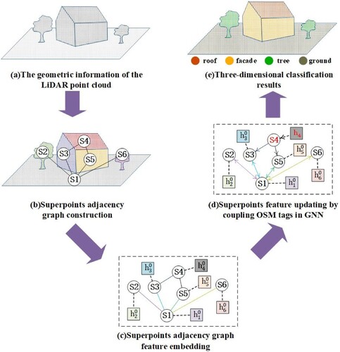
The proposed strategy, named as GNN with OSM data, for LiDAR point cloud classification consisted of three major parts, as illustrated in Figure 1. Firstly, LiDAR point cloud was over-segmented to construct a superpoint adjacency graph (From Figure 1(a,b)). This part aimed to define the appropriate primitives for performing semantic inference of the LiDAR point cloud after introducing the OSM data, and the derived superpoints were also used as the classification primitives. The superpoint adjacency graph was constructed based on the Euclidean adjacency relationship between superpoints (more details can be found in Section 2.1). Secondly, features were embedded for the superpoint adjacency graph (Figure 1(c)). As each superpoint contains a different number of points, they must be converted into feature vectors of the same dimension by feature embedding. Furthermore, the edges representing the adjacency relationship between superpoints need features that serve as weights when transmitting information in the GNN. More information about feature embedding is available in Section 2.2. Thirdly, the prior knowledge represented as labels tagged in OSM data was transmitted in the GNN. In this part, some superpoints (e.g. the superpoint S4 in Figure 1(c)) were associated with OSM data, and their hidden features were not updated to ensure their original prior knowledge transmitted in updating the hidden features of other superpoints (Figure 1(c)), which were further detailed in Section 2.3.

Figure 1. Illustrations of Light Detection and Ranging (LiDAR) point cloud classification strategy that incorporates tagged labels from OpenStreetMap (OSM) data into a graph neural network (i.e. the GNN with OSM data). (a) Diagram of the LiDAR point cloud of an urban scene. (b) Constructing a superpoint adjacency graph based on the result of over-segmentation. Points with same color represent a superpoint, denotated as a node S_i. (c) Embedding hidden features (i.e. $h_i^o$) for every node. (d) Updating the hidden features of superpoints after associating a part of the superpoints with OSM data (i.e. the red-colored node S4), (e) Classification of LiDAR point cloud using the updated hidden features.

2.1. LiDAR point cloud over-segmentation and superpoint adjacency graph construction

LiDAR point cloud is a discrete and disordered point set, lacking a simple grid structure as in remote sensing image. Therefore, the corresponding neighborhood is needed for point cloud in local feature perception. Furthermore, the intensive measurement by LiDAR sensors brings many redundant points into the descriptions of single geo-objects, for example, a building often contains hundreds of points. Therefore, a graph network built directly from the original LiDAR point cloud would be too complicated and would require an excessive amount of time in subsequent learning. Superpoints obtained from point cloud over-segmentation provide better primitives to construct the graph network. For example, in the illustration of the process in Figure 1(a,b), all LiDAR points were over-segmented into 6 superpoints for constructing a superpoint adjacency graph.

2.1.1. LiDAR point cloud over-segmentation based on graph cut

The over-segmentation of LiDAR point clouds generally assumes that point clouds of the same geo-objects have similar features. In this study, we used four features, represented as ${\mathit{f}}_{seg}\in {\mathbb{R}}^4$, which include linear, planar, volumetric, and vertical features. A more detailed explanation for the four features can be found in (Guinard and Landrieu 2017). Apart from satisfying the similarity of features, point cloud segmentation needs to conform to the connectivity between point clouds. This connectivity can be expressed by adjacency, that is, the set of edges $E$. Therefore, the optimization objective of over-segmentation can be regarded as the energy function of Potts segmentation, as shown in Equation (1): (1) $\begin{array}{c}{\mathit{g}}^{\ast }=\underset{\mathit{g}\in {\mathbb{R}}^{n\times 4}}{\arg min}\sum _i{\Vert {\mathit{g}}_i-{\mathit{f}}_{\left\{{\left\{\mathit{s}eg\right\}}_i\right\}}\Vert }^2+\lambda \sum _{\left(i,j\right)\in E}I\left({\mathit{g}}_i\ne {\mathit{g}}_j\right),\end{array}$(1) where $\left(i,j\right)\in E$ implies that the ith point is adjacent to the jth point. The optimization result ${\mathit{g}}^{\ast }$ is a tensor with repeated components, and the connected region of the same component is defined as the superpoint. The edge weight I is chosen to be linearly decreasing with respect to the edge length. $\lambda$ is a hyperparameter that expresses a compromise function between the number of partitions and the shape of the partitions. Although the hyperparameter $\lambda$ must be set in the segmentation process, the Potts segmentation does not require selecting the size and quantity of the partition in advance. Because the size of urban objects is difficult to determine, in other words, the ground is usually continuous over a large area while the trees are separated one by one, these circumstances make it very difficult to determine the size of partitions. Consequently, the Potts segmentation is particularly good for large-scale urban LiDAR point cloud segmentation. The Potts energy function can be solved approximately by the l₀-cut algorithm (Guinard and Landrieu 2017). Additionally, detailed discussion of the influence of the hyperparameter $\lambda$ on the segmentation results is provided in Section 4.1.

2.1.2. Constructing adjacency graph to express the relationship between superpoints

Theoretically, over-segmenting the LiDAR point cloud results in a set of independent superpoints. Therefore, the adjacency between the superpoints is needed for the subsequent processes. The adjacency between superpoints can be expressed by the graph structure,$\mathcal{G}=\left(\mathcal{V},\mathcal{E}\right)$, where $\mathcal{V}$ is the set of nodes or the set of superpoints, and $\mathcal{E}$ is the set of edges between the nodes, an expression of the adjacency between the superpoints. During the construction of the superpoint adjacency graph, to determine the adjacency between superpoints, we first determine the adjacency between the raw points using the Delaunay algorithm to construct a triangulation network containing all LiDAR points. If two raw points have an adjacency relationship, two superpoints containing the above-mentioned two raw points would also have an adjacency relationship. Furthermore, the edges connecting different superpoints in the Delaunay triangulation are screened out and added to the edge set $\mathcal{E}$ of the adjacency graph. The superpoints corresponding to the vertices of these edges are considered as having an adjacency relationship. The formula is as Equation (2): (2) $ϵ=\left\{\left(V,U\right)\in {\mathcal{V}}^2|\mathrm{\exists }\left(i,j\right)\in {\mathcal{E}}_{\mathrm{\Delta }}\cap \left(V\times U\right)\right\},$(2) where V and U are the superpoints, ${\mathcal{V}}^2$ is the set of all superpoint pairs, i and j are any points in the superpoints V and U, respectively, and ${\mathcal{E}}_{\mathrm{\Delta }}$ is the set of all edges in the Delaunay triangulation.

2.2. Feature embedding for superpoint adjacency graph

The superpoints constructed by over-segmentation have unequal sizes. For example, a superpoint belonging to ground generally contains more points than that belonging to a vehicle. The feature embedding aimed at these superpoints with unequal sizes have features with the same length. Several deep learning-based methods have been proposed for this purpose recently.

This study used PointNet due to its remarkable simplicity, efficiency, and robustness. PointNet defines a multilayer perceptron (MLP)-Max operation in a spherical neighborhood to extract point features (Qi et al. 2017). In the MLP-Max operation, an MLP is used on original attributes to extract deeper features for each point, and then maximum pooling is used to summarize the extracted features of all points within a superpoint into a single vector (i.e. embedded feature for the superpoint). Original attributes for each point include the geometric coordinates ($x,y,z$) and four geometric attributes describing linear, planar, volumetric and vertical characteristic. Additionally, during feature embedding, PointNet used another MLP to learn a rotation matrix for transforming the geometric coordinates to keep feature been rotation invariance.

The embedded features of superpoints (i.e. nodes) in the adjacency graph only express the characteristics of the superpoint, rather than the relationships between superpoints. These relationships need to be established based on the features of the adjacency graph. In this study, the features with 13 dimensions, as shown in Table 1, are used to represent the relationships.

Table 1. The edge features used in this study, with U, V representing the two adjacent superpoints.

Feature name	Eigenvector dimension	Specific meaning
Center distance	3	The distance between the central coordinates of U and V
Distance mean	3	The mean of the distances of all edges connecting U and V in the Delaunay triangulation
Distance variance	3	The variance of the distance of all edges connecting U and V in the Delaunay Triangulation
Point ratio	1	The ratio of the number of points in U and V
Geometric ratio	3	The ratio of linear, planar, and volumetric attributes calculated from the covariance matrix of U and V

2.3. Transmission of the information from OSM data in the GNN

2.3.1. Associating superpoints with OSM data

Considering the inference primitives in the GNN (i.e. superpoints), polygon geometries provided in OSM data are more suitable for introducing into the GNN than point and polyline geometries. Moreover, OSM data have many geometries with tagged labels, but its location precision may be poor. Therefore, this study only used building geometries tagged as ‘Tag: building = yes’ in OSM data (Figure 2(a)). The OSM data and LiDAR generally have specified spatial coordinates, and thus the superpoints and the building geometries can be easily aligned. Additionally, to further ensure accuracy of the associating process, we only associate a superpoint with OSM building information if it meets the following three criteria: (1) 80% of points in the superpoint should be covered by OSM building polygons; (2) the number of points in the superpoint (i.e. superpoint size) should be larger than 80; and (3) the maximum elevation between points in the superpoint should smaller than 3 m.

Figure 2. Information transmission from OSM data in the GNN. (a) Associating a part of superpoints with building polygon extracted from OSM data. (b) Fixing the hidden features of the superpoints with the associated building polygon. (c) Updating the hidden features of other superpoints without associated building polygons based on the gated recurrent unit. (d) Classification of LiDAR point cloud using the updated hidden features as shown in Figure 1(e).

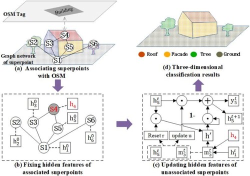
2.3.2. Transmission of the information from OSM data based on the gated recurrent unit

Transmission of the information from the associated OSM data is accomplished by fixing the hidden state of the superpoint associated with OSM, as shown in Figure 2(b). The state of the superpoints associated with the OSM building need not be updated; thus, the information from the OSM building can be used when updating the features of other superpoints. The basic unit used for updating the superpoint feature is the Gated Recurrent Unit (GRU), as shown in Figure 2(c). The initial state, ${\mathit{h}}_V^0$, of the superpoint is the feature embedded by PointNet in Section 2.2. Then ${\mathit{h}}_V^0$ is processed over several iterations (time steps) t = 0∼T. At each iteration t, a GRU takes its hidden state ${\mathit{h}}_V^{\left(t\right)}$ and an incoming message ${\mathit{m}}_V^t$ as input, and computes its new hidden state ${\mathit{h}}_V^{\left(t+1\right)}$.

The incoming message ${\mathit{m}}_V^t$ to superpoint V is computed as a weighted sum of the hidden states ${\mathit{h}}_U^{\left(t\right)}$ of neighboring superpoints U. The actual weighting for a superedge (U, V) depends on its attributes listed in Table 1. For example, ${\mathit{m}}_5^t$ refers to the influence of other superpoints on superpoint 5 in the graph network, i.e. it is the aggregation of the features of the adjacent nodes 1 and 4, which is associated with the OSM building. The aggregation method is as shown in Equation (3): (3) $\begin{array}{c}{\mathit{m}}_V^t=\mathrm{m}\mathrm{e}\mathrm{a}{\mathrm{n}}_{U\left|\right(V,U)\in \mathcal{E}}\left(\mathrm{M}\mathrm{L}{\mathrm{P}}_{\mathrm{e}\mathrm{d}\mathrm{g}\mathrm{e}}({\mathit{f}}_{VU}\right)\odot {\mathit{h}}_U^t),\end{array}$(3) where $\mathcal{E}$ is the edge from the superpoint adjacency graph in Section 2.1. $\mathrm{M}\mathrm{L}{\mathrm{P}}_{\mathrm{e}\mathrm{d}\mathrm{g}\mathrm{e}}$ converts the edge feature ${\mathit{f}}_{VU}$, into a vector consistent with the hidden state dimension for element-by-element multiplication such that information transmission and feature updating can be conducted effectively with the help of edge features.

2.3.3. Point cloud semantic category inference based on GNN with OSM data

During the GRU iteration, a series of hidden states, $\left(h_V^0,h_V^1,h_V^2,\dots ,h_V^t\right)$, is generated for each superpoint without associating OSM building polygons. These hidden states reflect the superpoint information at different iterative steps. A linear model can be used to map the hidden states generated in these iterative flows to the category space, as shown in Equations (4) and (5): (4) $\begin{array}{c}L\left(v\right)=W{\left(h_V^0,h_V^1,h_V^2,\dots ,h_V^t\right)}^T,\end{array}$(4) (5) $\begin{array}{c}\mathit{l}\left(c\right)=\underset{c\in \mathcal{L}}{\arg max}\mathit{L}\left(\mathit{v},c\right),\end{array}$(5) where $W$ is the parameter matrix of the linear model that needs to be trained, $\mathcal{L}$ is the category space, and $L\left(v\right)$ is the probability vector of the superpoint classification. The superpoint category, $l\left(c\right)$, is the category $c$ corresponding to the maximum probability.

3. Experimental data and result

3.1. Experimental data

The LiDAR point cloud used in this is an airborne LiDAR dataset that was collected by Leica Geosystems in Vaihingen using the Leica ALS50 system with a 45° field of view. Its geographic coordinate system is World Geodetic System 1984 (WGS84), and the projected coordinate system is Universal Transverse Mercator (UTM) zone 32N. The average point density is 8 pts/m². The ISPRS working group labeled some parts of these data as training and testing data to evaluate the 3D land cover classification, as shown in Figure 3. The labeled categories are power line, low vegetation, impervious surface, car, fence, roof, facade, shrub, and tree.

Figure 3. Data used in this study. (a) LiDAR training data. (b) LiDAR testing data. (c) Corresponding multispectral imagery of LiDAR training data. (d) Corresponding multispectral imagery of LiDAR testing data. (e) Building geometries from OSM data within LiDAR training data. (f) Building geometries from OSM data within LiDAR testing data.

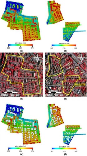
During the training processes of GNN with (or without) OSM data, we split the training dataset provided by the Vaihingen data set into the training data (i.e. 90% of all data) and validation data (i.e. the remaining 10% of all data). The validation data was used to evaluate the model’s performance in the training process and determine whether to stop the training process, which is shown in Figures 6 and 7. The accuracy of every category (Table 3) is evaluated using testing data provided by the Vaihingen data set, which does not include any part of the training dataset.

OSM includes spatial data as well as attribute data; in this case, spatial data consists of three main types: Nodes, Ways and Relations, which primitively make up the entire map picture. Nodes define the position of points in space; Ways define lines or areas; and Relations (optional) define the relationships between elements. Attribute data (Tags) are used to describe vector data primitives. Tags are not a basic element of the map, but the elements record information about the data through tags. The data is recorded through a ‘key’ and a ‘value’. For example, building geometries can be defined by ‘Tag: building = yes.’ The coordinate system used for the OSM tag is the geographic coordinate system WGS84, not the projected coordinate system. Thus, the OSM need to be transformed to UTM-32N such that it can be coupled and overlaid with LiDAR point cloud data in the same projection coordinate system. As mentioned in Section 2.3, this study only extracted building geometries from the OSM data.

3.2. The result of superpoint construction

Figure 4 shows the superpoints constructed after over-segmentation of the LiDAR point cloud. For the superpoints in the training data, the size and distributions are counted by category, as shown in Table 2. From Table 2, we know that the largest superpoint is impervious ground and the smallest superpoint is a power line, indicating that the discontinuity of power lines is more prominent in airborne LiDAR data. It is reasonable that the superpoints of impervious ground have the largest variance and the superpoints of automobiles have a smaller variance. From the frequency statistics of the data, it can be obtained that 50% of the superpoints contain less than 20 points (as shown in the row corresponding to 50%), and 90% of the superpoints contain no more than 100 point clouds, which means that only a very small number of superpoints have large continuous areas. A total of 525 superpoints were associated with OSM data, and 90% of these superpoints were building (including roof and façade), indicating that the associating process has high accuracy and can support the inference process in the GNN.

Figure 4. Results of superpoints constructed by over-segmentation.

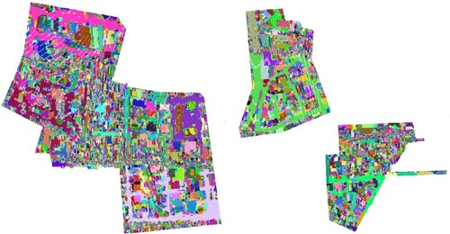
Table 2. Statistics of parameter of constructed superpoints for LiDAR training data.

		Power line	Low vegetation	Impervious surface	Car	Fence	Roof	Facade	Shrub	Tree
Total number		80	3416	2898	253	515	2769	1376	1852	3232
Mean of superpoint size		4.95	53.28	67.54	17.84	22.70	55.73	17.76	23.91	42.24
Variance of superpoint size		5.62	566.78	668.11	19.23	33.31	185.93	28.26	32.18	110.68
Number of superpoints associated with OSM data		0	24	3	1	0	417	58	3	18
Statistics of superpoint size at percentages	10%	1	2	3	2	1	2	1	1	1
	20%	1	7	11	3	2	8	2	2	4
	30%	2	11	13	7	4	12	3	6.3	10
	40%	2	14	14	11	10	14	6	11	14
	50%	2	17	17	14	13	18	10	14	18
	60%	3	22	20	16	17	23	14	19	24
	70%	4.3	30	26	21	23	32	19	25	32
	80%	9.2	45	34.6	25.6	35	50	26	35	46
	90%	13	89	70	42	52	106.2	40	54	86
	100%	30	32483	25541	189	336	5201	457	386	2848

3.3. Classification results of the GNN with OSM data

Table 3 shows the classification results of the GNN with OSM data along with the GNN without OSM data (i.e. the original GNN). We used three measures, precision, recall, and F1-score, to evaluate the results. F1-scores, the harmonic average of the precision and recall rates, indicate that the GNN with OSM data is generally better than the original GNN, except for low vegetation. In Table 3, we use bold to highlight the best F1-score for each category, and we mark the difference between the F1-score of the GNN with OSM data. The value of the difference is the F1-score of the GNN with OSM data minus the F1-score of the original GNN. It is noted, in particular, that the F1-score of the GNN with OSM data increased by 0.32% for roof, 2.15% for tree, and 2.96% for impervious surface. Thus, it is shown that the GNN with OSM data method is helpful to better identify other categories in addition to buildings.

Table 3. Assessment of classification results from original GNN and OSM-coupled GNN.

Category	Number of samples	GNN without OSM data (original GNN)			GNN with OSM data
		Precision	Recall	F1-score	Precision	Recall	F1-score
Power line	600	87.50%	01.17%	02.30%	78.38%	04.83%	09.11^+6^.^80%
Low vegetation	98690	69.55%	77.46%	73.29%	76.72%	64.56%	70.12^−3^.^17%
Impervious surface	101986	89.04%	74.91%	81.36%	78.99%	90.42%	84.32^+2^.^96%
Car	3708	49.35%	04.10%	07.57%	51.89%	05.93%	10.65^+3^.^08%
Fence	7422	53.50%	09.57%	16.23%	32.50%	24.05%	27.64^+11^.^41%
Roof	109048	88.73%	92.95%	90.79%	88.84%	93.52%	91.12^+0^.^32%
Facade	11224	68.36%	31.84%	43.45%	55.50%	40.04%	46.52^+3^.^07%
Shrub	24818	37.16%	49.50%	42.45%	35.90%	52.02%	42.49^+0^.^03%
Tree	54226	70.06%	79.92%	74.66%	82.59%	71.79%	76.81^+2^.^15%
Weighted mean	N/A	77.10%	76.33%	75.71%	77.21%	76.82%	76.38^+0^.^67%

Note: N/A represents not available.

4. Discussion

4.1. The influence of regularization strength $\lambda$ on the superpoint construction

The construction of the superpoints is significantly affected by the regularization strength $\lambda$. If a different regularization strength is used, the distribution of the superpoint size is different, as shown in Figure 5. The construction of the superpoints is evaluated by the number, reversibility, median (the median of the superpoint size), variance (an index to measure the difference between the size of the superpoints), minimum (the minimum number of points contained in a superpoint), and maximum (the maximum number of points contained in a superpoint). Reversibility is defined as the consistency between the category of the point obtained from the corresponding superpoint and the original category, which is measured by the F1-score.

Figure 5. Effect of the regularization strength $\lambda$ on superpoint construction.

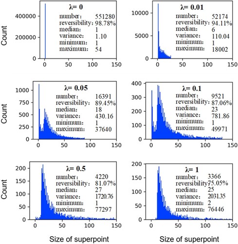
As shown by the segmentation results of these parameters, the number of superpoints decreases when the regularization strength increases. When the regularization strength is 0, the optimal value of the objective function is 0 if g in Equation (1) is equal to the feature of the original point. However, this study used the approximate solution of a graph cut. Thus, when the regularization strength is 0, the number of superpoints does not equal the number of original points, but the two are close. When the regularization strength is large enough, there is only g remaining, which tends to be consistent. In this case, all points are expressed as the same superpoint. However, this superpoint has very poor reversibility because of its large size, and the category of a single point cannot be restored from the category of the superpoint. Thus, considering these parameters comprehensively, the regularization strength of 0.05 is adopted in this study, which can not only obtain a better segmentation result but also provide better reversibility.

4.2. Analysis of training of the GNN with OSM data

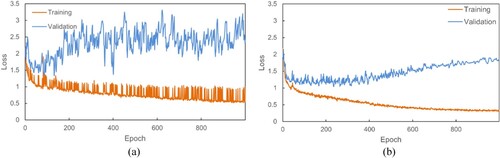
The GNN with OSM data training involves multiple hyperparameters, including the size of the superpoint during the feature embedding by PointNet, which is directly related to the data. As shown in Figure 5, when the regularization strength is greater than 0.05, the median of the superpoint is approximately 20. Therefore, we compare the difference when the threshold of the superpoint size is set to 10 and 20, as shown in Figure 6. When the superpoint size threshold is small, the loss of the GNN fluctuates significantly, making it difficult to converge, as shown in Figure 6(a), while the loss is relatively stable when the superpoint size threshold is set to 20, as shown in Figure 6(b). In other words, 50% of the superpoints are not features embedded by PointNet, but features obtained by the GNN.

Figure 6. Effect of loss on convergence when minimum superpoint size is set to 10 (a) and 20 (b).

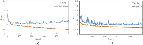
As we can see in Figure 6(b), although the training loss converges smoothly, the testing loss decreases slightly in the early stage but increases in the late stage, indicating overfitting in the GNN. The overfitting results primarily from the model being too powerful and the training data being insufficient, reflecting that the GNN depends heavily on the amount of data, like other deep learning algorithms. To avoid such overfitting, we add the dropout module and L2 regularization to the GNN, as shown in Figure 7. Adding the dropout module has only a limited effect on overfitting while adding the dropout module and L2 regularization more effectively prevents overfitting. The classification results in Section 3.3 show the case where both dropout and L2 regularization are used.

Figure 7. Effect on preventing overfitting: (a) with a dropout module and (b) with both dropout and L2 regularization.

4.3. Reasons for the improvement in accuracy after OSM coupling and implications for future work

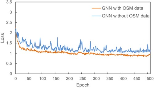
After coupling OSM into GNN, its performance on LiDAR point cloud classification is generally improved (Table 3). The improvement is also reflected in the decrease of loss in training processes (Figure 8). Compared with the GNN without OSM data, GNN with OSM data has stable loss convergence and lower loss value, which is the major reason for accuracy improvement of LiDAR point cloud classification. Theoretically, node features of GNNs usually tend to become more similar with the increase of the network depth (i.e. over-smoothing), which is the major bottleneck of GNNs and also exists in our used GNN (Rusch et al. 2023). In this study, after associating the OSM building information for some superpoints and fixing its feature in iterative update processes, the over-smoothing could be mitigated, resulting in an accuracy improvement. Based on our practice for integrating OSM building information into GNN, the information of other geo-objects from OSM data, such trees and roads, may also be used to improve the performance accuracy of the GNN model. However, unlike that, the building object in OSM data is a polygon, the tree object in OSM data is a point and the road object in OSM data is a polyline. Thus, associating these objects with superpoints in GNN should be done with caution, especially after considering their location accuracy. How to accomplish these association need to be further investigated. Additionally, this study has tried to introduce OSM data to the GNN method to improve its performance. Given the successful attempt, we think integrating OSM data with other state-of-the-art methods may also increase their accuracy on LiDAR point cloud.

Figure 8. Comparison between the loss decrease of the GNN with and without OSM data.

5. Conclusion

To better use the semantic information of the geo-objects contained in the crowd-sourced map OSM, we do not simply take it as the ground truth to train for deep learning. Instead, we coupled the OSM data into the LiDAR point cloud classification with the support of a GNN. In this study, the classification primitive was constructed by over-segmentation of the LiDAR point cloud. It is also the unit associated with the OSM data and with the building information contained in OSM. Compared with the original GNN, the GNN with OSM data achieves better performance in 8 out of 9 categories. This may be due to the introduction of prior information, which avoids inconsistency in the GNN transfer and makes the learning process more focused on other indistinguishable geo-objects. Furthermore, after over-segmenting the LiDAR point clouds, approximately 50% of superpoints contained less than 20 points. This indicates that the over-segmentation results of low-density airborne LiDAR point clouds are too sparse, which limits feature embedding in the GNN. In addition, the dropout module and regularization can avoid GNN overfitting. Urban geo-objects have a special relationship with each other. The classification would be more intelligent by embedding that potential relationship. The development of innovative reasoning models in the field of artificial intelligence, especially the development of GNNs and knowledge graphs, can provide a new perspective for point cloud semantic classification.

Acknowledgements

The authors are grateful to the editors and the anonymous reviewers for their valuable comments and suggestions.

Disclosure statement

No potential conflict of interest was reported by the author(s).

Data availability statement

The Vaihingen data set was provided by the German Society for Photogrammetry, Remote Sensing and Geoinformation (DGPF): http://www.ifp.uni-stuttgart.de/dgpf/DKEPAllg.html. The LiDAR point cloud were provided by the International Society for Photogrammetry and Remote Sensing (ISPRS): https://www.isprs.org/education/benchmarks.aspx. OSM was downloaded from https://www.opestreetmap.org/#map=15/48.9288/8.9638&layers=N.

Additional information

Funding

This work was supported by the National Natural Science Foundation of China (42071440), the National Key R&D Program of China (2023YFC3006701), the Natural Science Foundation of Jiangsu Province of China (BK20201257), the Open Fund of Key Laboratory of Urban Land Resources Monitoring and Simulation, Ministry of Natural Resources (KF-2021-06-004), the Key Laboratory of Spatial-temporal Big Data Analysis and Application of Natural Resources in Megacities, MNR (KFKT-2022-09), and the Fundamental Research Funds for the Central Universities of China (B210201049).

References

- Boulch, A. 2020. “ConvPoint: Continuous Convolutions for Point Cloud Processing.” Computers & Graphics 88 (5): 24–34. https://doi.org/10.1016/j.cag.2020.02.005.
- Chen, X., L. Li, F. Li, and A. Gupta. 2018. “Iterative Visual Reasoning Beyond Convolutions". In 2018 IEEE/CVF Conference on Computer Vision and Pattern Recognition. Salt Lake City, UT, USA. 18-23 June 2018.
- Elhousni, M., Z. Zhang, and X. Huang. 2022. “LiDAR-OSM-Based Vehicle Localization in GPS-Denied Environments by Using Constrained Particle Filter.” Sensors 22 (14): 5206–5221. https://doi.org/10.3390/s22145206.
- Fonte, C. C., J. A. Patriarca, M. Minghini, V. Antoniou, L. See, and M. A. Brovelli. 2019. “Using Openstreetmap to Create Land use and Land Cover Maps: Development of an Application.” In Geospatial Intelligence: Concepts, Methodologies, Tools, and Applications, edited by Information Resources Management Association, 1100–1123. Hershey, PA: IGI Global. https://doi.org/10.4018/978-1-5225-8054-6.ch047.
- Guinard, S., and L. Landrieu. 2017. “Weakly Supervised Segmentation-aided Classification of Urban Scenes from 3dLiDAR Point Clouds.” The International Archives of the Photogrammetry, Remote Sensing and Spatial Information Sciences XLII-1/W1: 151–157. https://doi.org/10.5194/isprs-archives-XLII-1-W1-151-2017.
- Guo, Y., H. Wang, Q. Hu, H. Liu, L. Liu, and M. Bennamoun. 2021. “Deep Learning for 3D Point Clouds: A Survey.” IEEE Transactions on Pattern Analysis and Machine Intelligence 43 (12): 4338–4364. https://doi.org/10.1109/TPAMI.2020.3005434.
- He, Y., H. Yu, X. Liu, Z. Yang, W. Sun, Y. Wang, Q. Fu, Y. Zou, and A. Mian. 2021. “Deep Learning Based 3D Segmentation: A Survey.” arXiv preprint. https://doi.org/10.48550/arXiv.2103.05423.
- Jiang, M., Y. Wu, T. Zhao, Z. Zhao, and C. Lu. 2018. “Pointsift: A Sift-like Network Module for 3D Point Cloud Semantic Segmentation.” arXiv preprint. https://doi.org/10.48550/arXiv.1807.00652.
- Khanal, N., M. A. Matin, K. Uddin, A. Poortinga, F. Chishtie, K. Tenneson, and D. Saah. 2020. “A Comparison of Three Temporal Smoothing Algorithms to Improve Land Cover Classification: A Case Study from NEPAL.” Remote Sensing 12 (18): 2888–2912. https://doi.org/10.3390/rs12182888.
- Landrieu, L., and M. Simonovsky. 2018. “Large-Scale Point Cloud Semantic Segmentation with Superpoint Graphs". In 2018 IEEE/CVF Conference on Computer Vision and Pattern Recognition . Salt Lake City, UT, USA. 18-23 June 2018.
- Lang, I., M. Asaf, and A. Shai. 2020. “Samplenet: Differentiable Point Cloud Sampling". In 2020 IEEE/CVF Conference Computer Vision and Pattern Recognition (CVPR). Seattle, WA, USA. 13-19 June 2020.
- Lei, T., L. Li, Z. Lv, M. Zhu, X. Du, and A. K. Nandi. 2021. “Multi-Modality and Multi-Scale Attention Fusion Network for Land Cover Classification from VHR Remote Sensing Images.” Remote Sensing 13 (18): 3771–3788. https://doi.org/10.3390/rs13183771.
- Li, N., C. Liu, and N. Pfeifer. 2019. “Improving LiDAR Classification Accuracy by Contextual Label Smoothing in Post-Processing.” ISPRS Journal of Photogrammetry and Remote Sensing 148: 13–31. https://doi.org/10.1016/j.isprsjprs.2018.11.022.
- Lin, Y., Z. Yan, H. Huang, D. Du, L. Liu, S. Cui, and X. Han. 2020. “FPConv: Learning Local Flattening for Point Convolution". In 2020 IEEE/CVF Conference on Computer Vision and Pattern Recognition (CVPR). Seattle, WA, USA. 13-19 June 2020.
- Liu, P., J. Zhang, C. Leung, C. He, and T. L. Griffiths. 2018. “Exploiting Effective Representations for Chinese Sentiment Analysis Using a Multi-channel Convolutional Neural Network.” arXiv preprint. https://doi.org/10.48550/arXiv.1808.02961.
- Pazoky, S. H., and P. Pahlavani. 2021. “Developing a Multi-Classifier System to Classify OSM Tags Based on Centrality Parameters.” International Journal of Applied Earth Observation and Geoinformation 104: 102595. https://doi.org/10.1016/j.jag.2021.102595.
- Qi, C. R., H. Su, K. Mo, and L. J. Guibas. 2017. “Pointnet: Deep Learning on Point Sets for 3D Classification and Segmentation". In 2017 IEEE Conference on Computer Vision and Pattern Recognition (CVPR). Honolulu, HI, USA. 21-26 July 2017.
- Qi, C. R., L. Yi, H. Su, and L. J. Guibas. 2017. “PointNet++: Deep Hierarchical Feature Learning on Point Sets in a Metric Space.” arXiv preprint. https://doi.org/10.48550/arXiv.1706.02413.
- Rusch, T. K., M. M. Bronstein, and S. Mishra. 2023. “A Survey on Oversmoothing in Graph Neural Networks.” arXiv preprint. https://doi.org/10.48550/arXiv.2303.10993.
- Sklyar, E., and G. Rees. 2022. “Assessing Changes in Boreal Vegetation of Kola Peninsula via Large-Scale Land Cover Classification Between 1985 and 2021.” Remote Sensing 14 (21): 5616–5637. https://doi.org/10.3390/rs14215616.
- Solórzano, J. V., J. F. Mass, Y. Gao, and J. A. Gallardo-Cruz. 2021. “Land Use Land Cover Classification with U-Net: Advantages of Combining Sentinel-1 and Sentinel-2 Imagery.” Remote Sensing 13 (18): 3600–3622. https://doi.org/10.3390/rs13183600.
- Wang, X., J. Cao, J. Liu, X. Li, L. Wang, F. Zuo, and M. Bai. 2022. “Improving the Interpretability and Reliability of Regional Land Cover Classification by U-Net Using Remote Sensing Data.” Chinese Geographical Science 32 (6): 979–994. https://doi.org/10.1007/s11769-022-1315-z.
- Wang, L., Y. Huang, Y. Hou, S. Zhang, and J. Shan. 2019. “Graph Attention Convolution for Point Cloud Semantic Segmentation". In 2019 IEEE/CVF Conference on Computer Vision and Pattern Recognition (CVPR). Long Beach, CA, USA. 15-20 June 2019.
- Wang, Y., D. Tan, N. Navab, and F. Tombari. 2020. “Softpoolnet: Shape Descriptor for Point Cloud Completion and Classification". In European Conference on Computer Vision. Glasgow, UK. August 23-28, 2020.
- Wang, C., X. Wang, D. Wu, M. Kuang, and Z. Li. 2022. “Meticulous Land Cover Classification of High-Resolution Images Based on Interval Type-2 Fuzzy Neural Network with Gaussian Regression Model.” Remote Sensing 14 (15): 3704–3728. https://doi.org/10.3390/rs14153704.
- Xu, Q., X. Sun, C. Wu, P. Wang, and U. Neumann. 2020. “Grid-GCN for Fast and Scalable Point Cloud Learning". In 2020 IEEE/CVF Conference on Computer Vision and Pattern Recognition (CVPR). Seattle, WA, USA. 13-19 June 2020.
- Xue, H., C. Liu, F. Wan, J. Jiao, X. Ji, and Q. Ye. 2019. “Danet: Divergent Activation for Weakly Supervised Object Localization". In 2019 IEEE/CVF International Conference on Computer Vision (ICCV). Seoul, Korea (South). 27 October 2019 - 02 November 2019.
- Yan, X., C. Zheng, Z. Li, S. Wang, and S. Cui. 2020. “Pointasnl: Robust Point clouds Processing Using Nonlocal Neural Networks with Adaptive Sampling". In 2020 IEEE/CVF Conference on Computer Vision and Pattern Recognition (CVPR). Seattle, WA, USA. 13-19 June 2020.
- Zhao, J., L. Wang, H. Yang, P. Wu, B. Wang, C. Pan, and Y. Wu. 2022. “A Land Cover Classification Method for High-Resolution Remote Sensing Images Based on NDVI Deep Learning Fusion Network.” Remote Sensing 14 (21): 5455–5473. https://doi.org/10.3390/rs14215455.
- Zhou, H., Y. Feng, M. Fang, M. Wei, J. Qin, and T. Lu. 2021. “Adaptive Graph Convolution for Point Cloud Analysis". In 2021 IEEE/CVF International Conference on Computer Vision (ICCV). Montreal, QC, Canada. 10-17 October 2021.
- Zhou, Q., Y. Zhang, K. Chang, and M. A. Brovelli. 2022. “Assessing OSM Building Completeness for Almost 13,000 Cities Globally.” International Journal of Digital Earth 15 (1): 2400–2421. https://doi.org/10.1080/17538947.2022.2159550.