Comparative study on information extraction of urban wetlands and its thermal environment using the SDGSAT-1 data

ABSTRACT

Wetlands represent crucial ecosystems, with urban wetlands playing a significant role in regulating regional thermal environments. The Sustainable Development Goals Scientific Satellite 1 (SDGSAT-1), equipped with multiple sensors, boasts one of the highest spatial resolutions among satellites housing thermal infrared sensors. A specific deep blue band, sensitive to chlorophyll in water, has been established, introducing innovative technological avenues for observing urban wetland environments. This study focuses on Beijing, investigating SDGSAT-1's efficacy in wetland classification and Land Surface Temperature (LST) retrieval, in comparison to Sentinel-2 and Landsat 8 TIRS data. The findings reveal that: (1) Wetland classification accuracy with SDGSAT-1 (86.76% overall accuracy, 0.84 Kappa coefficient, 0.87 Macro-F1) surpasses that of Sentinel-2, possibly attributed to the deep blue bands; (2) In contrast to Landsat 8's thermal infrared band, SDGSAT-1's finer resolution (30 m spatial resolution) offers more intricate spatial variation of LST, forming a foundational dataset for nuanced wetland thermal environment investigations; (3) The study underscores the comprehensive advantages of SDGSAT-1 data in monitoring urban wetlands and thermal environments, furnishing a theoretical basis for future related research.

KEYWORDS:

• SDGSAT-1
• urban wetlands
• thermal environment
• comparative study

1. Introduction

Over recent decades, global urban areas, particularly in developing countries, have witnessed rapid expansion. This urbanization has given rise to the Urban Heat Island (UHI) effect, a phenomenon resulting from the replacement of natural landscapes with artificial surfaces. This transformation induces excessive heat storage and delayed nighttime release (Oke 1973), directly and indirectly impacting energy consumption, environmental quality, and human health (Aboelata 2020; He et al. 2021). Urban wetlands constitute vital natural resources in cities, offering diverse ecosystem regulation services (Alikhani, Nummi, and Ojala 2021; Rao et al. 1999; X. Yang et al. 2021). The cooling capacity inherent in wetlands contributes to the formation of an Urban Cool Island (UCI) effect within cities (Cao et al. 2010; Chang, Li, and Chang 2007), delivering substantial cooling effects to surrounding areas to alleviate the escalating Urban Heat Island (UHI) effect (Manteghi, Lamit, and Ossen 2015; R. Sun et al. 2012).

Accurately acquiring information on urban wetlands and their thermal environment is a prerequisite for understanding wetlands’ role in regulating urban microclimates and aiding in urban ecological construction. Remote sensing and GIS technologies, in comparison to traditional temperature measurement techniques, have gained prominence in recent studies on the UHI and UCI effects (Rasul et al. 2017; Voogt and Oke 2003). Substantial advancements in satellite sensor technology and the evolution of machine automated classification algorithms have notably progressed wetland mapping. Landsat and MODIS satellite data, with their extensive observational history, are frequently employed for large-scale, long-term studies (Chen et al. 2016; Niu et al. 2009; Xing and Niu 2019; Yin et al. 2024). The China High-resolution Earth Observation System (CHEOS) program and the Copernicus Programme have introduced high spatiotemporal resolution satellite data, enhancing wetland delineation and classification accuracy (Yang Li and Niu 2022; Zhang et al. 2022). Additionally, the integration of hyperspectral data and sophisticated deep learning algorithms has enriched spectral information and data mining capabilities, refining wetland mapping precision (Fu et al. 2023; Huang et al. 2023; Liu et al. 2022; W. Sun et al. 2023). In thermal environment information extraction, early use of NOAA AVHRR data for urban LST and UHI effect analysis has transitioned to the high temporal resolution capabilities of the MODIS sensor (Lazzarini, Marpu, and Ghedira 2013; Lee 1993; Streutker 2002), enabling diurnal LST and UHI analysis as well as global-scale city assessments (Clinton and Gong 2013). Landsat series images are extensively utilized to assess the relationship between LST and land use/land cover (LULC) and investigate wetland cooling capacity mechanisms (Bajaj, Inamdar, and Vaibhav 2012; Du et al. 2016; Wang and Zhu 2011; Y. Li, Zhang, and Kainz 2012; Y. Xu, Qin, and Lv 2008). Data from the ASTER sensor, which has a higher spatial resolution (90 m), has been used to explore landscape heterogeneity of urban heat islands and quantify the cooling capacity of wetlands (Buyantuyev and Wu 2010; R. Sun et al. 2012).

Despite these advancements, the diverse landscape types and spatial tessellation patterns in urban areas create complex energy balance and microclimate systems, resulting in substantial temperature variations within cities (Buyantuyev and Wu 2010). The dispersed nature of urban landscapes often leads to smaller characteristic spatial scales for water bodies and vegetation. High spatial resolution multispectral and thermal infrared image data are crucial for mapping complex land cover and detecting changes in urban wetland systems at local scales, offering a more realistic assessment of the wetland cool island effect (Cao et al. 2010; Lo, Quattrochi, and Luvall 1997; Voogt and Oke 2003; Zhou et al. 2010). However, current satellite data faces challenges in meeting these requirements.

The Sustainable Development Science Satellite 1 (SDGSAT-1) (Guo et al. 2023) stands as the world’s inaugural scientific satellite dedicated to advancing the United Nations 2030 Agenda for Sustainable Development. In response to the global imperative for monitoring SDGs, evaluating progress, and conducting scientific research, SDGSAT-1 is equipped with three payloads: Thermal Infrared Spectrometer (TIS), Glimmer Imager (GLI), and Multispectral Imager (MSI). GLI and MSI exhibit a spatial resolution of 10 m, while TIS boasts a spatial resolution of 30 m, ranking among the world's highest spatial resolution thermal infrared sensors. The full-time coordinated observation mode of SDGSAT-1's three payloads facilitates simultaneous acquisition of surface cover and temperature information, holding significant potential for research in wetland thermal environments, albeit still in its early stages. To evaluate the efficacy of SDGSAT-1 data in monitoring urban wetlands and its ability to elucidate the relationship between human activities and natural environments, a comparative study was conducted using Beijing city as the study area. The multispectral and thermal infrared bands of SDGSAT-1 were employed for urban wetland mapping and LST retrieval. Concurrently, Sentinel-2 data was utilized for urban wetland classification, and Landsat 8 TIRS data from the same date was employed for urban LST retrieval. Ultimately, a comprehensive exploration of the strengths and weaknesses of SDGSAT-1 data in wetland thermal environment research, in comparison to commonly used existing satellite data, was undertaken.

2. Study area and data

2.1. Study area

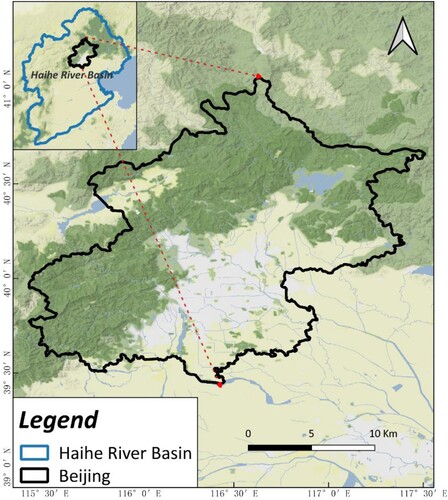
Beijing, situated in northern China and serving as the capital (Figure 1). It covers an area of 16,410 km² and is located between 39°28′N ∼ 41°05′N and 115°25′E ∼ 117°30′E, standing as the largest city in northern China. With a dense population and undergoing rapid urbanization (urbanization rate of 87.5%), Beijing faces a growing UHI effect, emerging as a critical environmental threat significantly impacting the health of its densely populated residents and the local environment (Kuang et al. 2015; T. Li, Xu, and Yao 2021). The urban thermal environment in Beijing displays evident spatiotemporal heterogeneity (Yao, Xu, and Zhang 2019). Stretching from west to east, Beijing encompasses five natural river channels: Juma River, Yongding River, North Canal, Chaobai River, and Ji Canal, all falling within the Haihe River Basin. Due to historical and contemporary urban planning considerations, the city hosts numerous artificial lakes, paddy fields, and various wetland types. These wetlands predominantly exist in the form of wetland parks, representing typical areas for investigating the thermal environmental effects of urban wetlands.

Figure 1. Map showing the location of the study area.

2.2. Data

2.2.1. Image data

Considering the imperative for wetland classification during the vegetation growth season and taking into account the data quality and availability of SDGSAT-1, this study meticulously screened the satellite images captured by SDGSAT-1 in 2022. Ultimately, six multispectral images were chosen, corresponding to specific imaging dates: February 1st (2 images), February 22nd (1 image), March 5th (1 image), and April 1st (2 images). The selected data, classified as L4 level, underwent essential processing steps, including radiometric correction, band registration, and orthorectification. Additionally, two thermal infrared images from April 1st were selected for further analysis, sharing the same L4 data level. For comprehensive details regarding the data source, refer to Table 1.

Table 1. Parameters of SDGSAT-1 data.

Categories of sensors	Indicator items	Specific indicators
Thermal Infrared Spectrometer	Detection spectrum	B1: 8∼10.5 μm
		B2: 10.3∼11.3 μm
		B3: 11.5∼12.5 μm
	Pixel resolution	30 m
	Time of acquisition	1 February 2022 22 February 2022 5 March 2022 1 April 2022
Multispectral Imager	Detection spectrum	B1: 374∼427 nm B2: 410∼467 nm B3: 457∼529 nm B4: 510∼597 nm B5: 618∼696 nm B6: 744∼813 nm B7: 798∼911 nm
	Pixel resolution	10 m
	Time of acquisition	1 April 2022

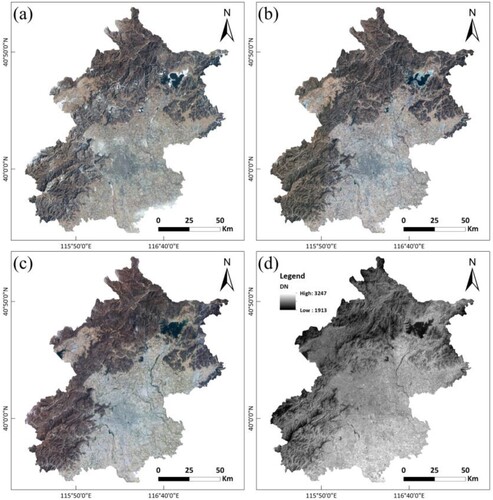
We employed ENVI 5.6 software for radiometric calibration, mosaicking, and clipping of images taken in the same month. This process resulted in three multispectral images that cover the entire Beijing area in February, March, and April 2022, along with a thermal infrared image encompassing the entire Beijing area on April 1st (Figure 2).

Figure 2. Selected multispectral images of SDGSAT-1 in (a) February, (b) March, (c) April, and thermal infrared image on (d) 1st April.

We chose Sentinel-2 Surface Reflectance data with a spatial resolution matching that of SDGSAT-1 multispectral data for evaluating wetland classification capabilities. This study utilized the Google Earth Engine cloud computing platform (Gorelick et al. 2017) to screen a total of 26 images on February 1st, March 3rd, March 5th, and April 2nd, closely aligning with the dates of SDGSAT-1 data. The data underwent the same pre-processing steps as SDGSAT-1, resulting in three Sentinel-2 multispectral images covering the entire Beijing area.

To assess the reliability of SDGSAT-1 thermal infrared sensor data in wetland thermal environment research, we employed Landsat 8 TIRS sensor data. An image from April 3rd was chosen and subjected to preprocessing steps, including radiometric calibration and cropping.

2.2.2. Sample data

The sample data in this study was generated through two methods. Firstly, high-resolution Google Earth images were utilized for manual visual interpretation. Secondly, existing datasets were employed for production. Specifically, Copernicus Global Land Cover Layers (Buchhorn et al. 2020, 2) and ESA WorldCover (Zanaga et al. 2022), two global land cover products, were used to identify randomly generated sample points. If both products determined the same category for a given sample point, the point was retained and assigned to the corresponding category; otherwise, it was discarded. In the study area, we independently selected training and testing data in a 7:3 ratio, resulting in a total of 3281 sample points.

3. Methods

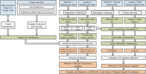
In this study, we devised a method to analyze the thermal environment of urban wetlands by integrating wetland mapping and LST retrieval. The method comprises two primary components. The initial segment involves wetland and land cover classification using multispectral data from SDGSAT-1 and Sentinel-2, respectively. The classification outcomes from these datasets are evaluated for accuracy to gauge the performance of SDGSAT-1 and conduct a comprehensive analysis. The subsequent phase entails temperature retrieval based on thermal infrared data from SDGSAT-1 and Landsat 8. Additionally, wetland thermal environment characteristics are extracted using the retrieval results. The accuracy of the retrieval and the precision of feature extraction undergo evaluation. The detailed process is illustrated in Figure 3.

Figure 3. Overall workflow of this paper.

3.1. Wetland classification methods

3.1.1. Wetland classification system

Referring to the Ramsar Convention and considering the specific distribution of wetlands in the study area, we formulated the wetland classification scheme outlined in Table 2.

Table 2. Wetland classification scheme.

First level	Second level	Specific instructions	Image example
Wetland	Water	Natural or artificial waters with water all year round (Lakes, rivers, reservoirs, etc.).
	Marsh	Soils are often saturated with water, the surface is permanently or temporarily waterlogged, wet and boggy plants are growing, peat is accumulating or there is no peat accumulation but a submerged layer exists.
	Paddy field	Arable land where water can accumulate for growing rice.
Non-wetland	Impervious surface	Surfaces covered by various impermeable building materials, such as roofs, roads and plazas made of tiles, asphalt, cement concrete, etc.
	Forest and Scrub	Biomes dominated by woody plants or shrubs.
	Grassland	Biomes dominated by herbaceous plants.
	Farmland	Refers to arable land other than paddy fields, including watered land and dry land without watering conditions.

3.1.2. Classification features

In comparison, one of the most noteworthy distinctions between SDGSAT-1 and Sentinel-2 lies in their band settings. SDGSAT-1 incorporates two additional deep blue bands compared to Sentinel-2: Band 1 and Band 2, while Sentinel-2 integrates three extra red-edge bands, namely Band 5, Band 6, and Band 8A, along with two more short-wave infrared bands, Band 11 and Band 12 (the Aerosols band and Water vapor band are not utilized as research data in this paper). Consequently, this study will scrutinize and assess the disparities in wetland classification capabilities between the two data sources based on these variances in band settings. To conduct the comparison, we initially select seven bands from each SDGSAT-1 image captured in February, March, and April 2022 as spectral features. For Sentinel-2 data, ten bands from each image are chosen as spectral features. Subsequently, index features are computed using their respective spectral features. Furthermore, both datasets incorporate terrain features calculated from the SRTM digital elevation data (Farr et al. 2007) provided by NASA. SDGSAT-1 utilizes a total of 49 features, while Sentinel-2 incorporates a total of 58 features, as depicted in Table 3.

Table 3. Description of the feature set.

Features variables	Name of the features	Calculation formulas
Spectral features	Band (SDGSAT-1)	Band1, Band2, Band3, Band4, Band5, Band6, Band7
	Band (Sentinel-2)	Band2, Band3, Band4, Band5, Band6, Band7, Band8, Band8A, Band11, Band12
Index features	Normalized Difference Vegetation Index (NDVI) (Rouse et al. 1974)	${\displaystyle \frac{\mathrm{Nir}-\mathrm{Red}}{\mathrm{Nir}+\mathrm{Red}}}$
	Normalized Difference Water Index (NDWI) (McFeeters 1996)	${\displaystyle \frac{\mathrm{Green}-\mathrm{Nir}}{\mathrm{Green}+\mathrm{Nir}}}$
	Blue-normalized difference vegetation index (BNDVI) (C. Yang et al. 2004)	${\displaystyle \frac{\mathrm{Nir}-\mathrm{Blue}}{\mathrm{Nir}+\mathrm{Blue}}}$
	Enhanced Vegetation Index (EVI) (A. Huete et al. 2002)	${\displaystyle \frac{\mathrm{Nir}-\mathrm{Red}}{\mathrm{Nir}+6\ast \mathrm{Red}-7.5\ast \mathrm{Blue}+1}}$
	Renormalized Difference Vegetation Index (RDVI) (Roujean and Breon 1995)	${\displaystyle \frac{\mathrm{Nir}-\mathrm{Red}}{\sqrt{\mathrm{Nir}+\mathrm{Red}}}}$
	Transformed Chlorophyll Absorption in Reflectance Index (TCARI) (Haboudane et al. 2002)	$3\times \left[\begin{array}{c}(\mathrm{Nir}-\mathrm{Red})-0.2\times \\ (\mathrm{Nir}-\mathrm{Green})\times \left({\displaystyle \frac{\mathrm{Nir}}{\mathrm{Red}}}\right)\end{array}\right]$
	Triangular Vegetation Index(TVI) (Broge and Leblanc 2001)	$0.5\times \left[\begin{array}{c}120\times (\mathrm{Nir}-\mathrm{Green})-\\ 200\times (\mathrm{Red}-\mathrm{Greenn})\end{array}\right]$
	Soil Adjusted Vegetation Index (SAVI) (A. R. Huete 1988)	${\displaystyle \frac{1.5\times (\mathrm{Nir}-\mathrm{Red})}{\mathrm{Nir}+\mathrm{Red}+0.5}}$
Terrain Features	Elevation
	Slope
	Aspect
	Hillshade

To assess the quality of the chosen classification features and sample points, we utilized the Jeffries-Matusita (JM) distance to quantify the separability of different category samples based on the selected classification features. The JM distance has been established as an effective measure for evaluating separability among diverse samples or features (Dabboor et al. 2014; Garcia Salgado and Ponomaryov 2015; Sen, Goswami, and Chakraborty 2019). A larger JM distance indicates a smaller similarity between categories, with its value range being [0, 2]. Typically, a JM distance exceeding 1.8 is considered indicative of good separability between samples, and a value of 2 signifies complete separation between two categories based on the selected features. As illustrated in Table 4, the selected samples in this study demonstrate good separability concerning the chosen SDGSAT-1 classification features. Furthermore, the JM distance will be employed to evaluate the separability between wetland and non-wetland categories across individual bands of SDGSAT-1 multispectral data. This approach aims to identify the most suitable band for wetland classification.

Table 4. JM distance between different class samples.

Categories	Water	Marsh	Paddy field	Impervious surface	Forest and Scrub	Grassland	Farmland
Water	0	1.99998	2	2	2	2	2
Marsh		0	2	1.99990	1.99988	1.99999	1.99986
Paddy field			0	1.99994	2	2	1.99914
Impervious surface				0	1.99989	1.99987	1.99215
Forest and Scrub					0	1.97254	1.99934
Grassland						0	1.99919
Farmland							0

3.1.3. Classification algorithm

The Boosting algorithm (Freund, Schapire, and Abe 1999) is a technique for constructing a robust classifier by aggregating multiple weak classifiers. It effectively mitigates bias and variance, enhancing generalization capabilities. The Boosting method trains base classifiers sequentially, with interdependencies among them. Its fundamental concept involves stacking the base classifiers layer by layer. During each layer's training, higher weights are assigned to samples misclassified by the previous layer's base classifier. During testing, the final result is determined based on the weighted outcomes of each layer's classifier. Numerous variants and enhancements of the Boosting algorithm exist, and these have demonstrated success in remote sensing image classification (Nowakowski 2015; Zhong, Hu, and Zhou 2019). In this study, we employ the GBDT (Gradient Boosting Decision Tree) (Friedman 2001) algorithm integrated on the Google Earth Engine platform for classification.

3.2. The retrieval and analysis method of LST

3.2.1. Retrieval algorithm of LST

This study employs the Radiative Transfer Equation (RTE) (Sobrino, Jiménez-Muñoz, and Paolini 2004, 5) to derive LST. LST retrieval is conducted using the B2 band of the SDGSAT-1 thermal infrared sensor data and the B10 band of Landsat 8. Initially, the thermal infrared image undergoes radiometric calibration to convert DN values into radiance (L_sensor): (1) $L_{\mathrm{sensor}}=\mathrm{DN}\times \mathrm{Gain}+\mathrm{Bias}$(1) Where Gain and Bias both come from the calibration file of the SDGSAT-1 data product. Next, calculate the spectral radiance of the ground surface (L): (2) $L={\displaystyle \frac{L_{\mathrm{sensor}}-L_{\mathrm{up}}}{\mathrm{\tau \epsilon }}-{\displaystyle \frac{(1-\epsilon )L_{\mathrm{down}}}{\epsilon }}}$(2) Where L_up and L_down are the upwelling and downwelling atmospheric radiation, respectively, and τ is the atmospheric transmittance. These three parameters can be obtained by entering the relevant parameters on the USGS atmospheric correction parameter query website (https://atmcorr.gsfc.nasa.gov/); ϵ is the surface emissivity, and the calculation method is as follows: (3) ${\epsilon }_{\mathrm{water}}=0.995$(3) (4) ${\epsilon }_{\mathrm{surface}}=0.9625+0.0614\mathrm{FVC}-0.0461\mathrm{FV}{C}^2$(4) (5) ${\epsilon }_{\mathrm{building}}=0.9589+0.086\mathrm{FVC}-0.0671\mathrm{FV}{C}^2$(5)

Among them, ϵ_water, ϵ_surface and ϵ_building are the emissivity of the water body, natural surface and building respectively. FVC is the Fractional Vegetation Cover: (6) $\mathrm{FVC}={\displaystyle \frac{\mathrm{NDVI}-\mathrm{NDV}{I}_{\mathrm{soil}}}{\mathrm{NDV}{I}_{\mathrm{veg}}-\mathrm{NDV}{I}_{\mathrm{soil}}}}$(6) Among them, $\mathrm{NDV}{I}_{\mathrm{veg}}$ represents the NDVI value of pixels completely covered by vegetation, that is, the NDVI value of pure vegetation pixels; $\mathrm{NDV}{I}_{\mathrm{soil}}$ represents the NDVI value of pixels that are completely bare soil or uncovered by vegetation(M. Li 2003). Finally, the surface temperature T is calculated: (7) $T={\displaystyle \frac{{10}^6\cdot \mathrm{hc}/(\mathrm{k}\lambda )}{\ln \left[2\cdot {\displaystyle \frac{{10}^{24}\mathrm{h}{\mathrm{c}}^2}{L{\lambda }^5}+1}\right]}}$(7) Among them, h is the Planck constant, with a value of 6.626×10–34 and a unit of J·s. c is the speed of light, with a value of 2.9979×108 and a unit of m s⁻¹. k is the Boltzmann constant, with a value of 1.3806×10–23 and a unit of J K⁻¹. λ is the central wavelength of the band.

3.2.2. Analysis method of wetland thermal environment

In this study, five representative wetlands were selected from the wetland classification results of SDGSAT-1 data: Beihai Park, Cuihu Park, Miyun Reservoir, Olympic Forest Park, and Yuyuantan Park. Utilizing the spatial analysis function in ArcGIS software, continuous buffer zones were established around each wetland at intervals of 50 m. The average LST within each buffer zone was computed, and the LST curves for the five wetlands were graphed. Subsequently, relevant indicators for each wetland were calculated, as detailed in Table 5. Since the surface temperature around the wetland may be influenced by urban heat sources or other adjacent wetlands, these influences can result in irregular fluctuations in the temperature curve, impacting the curve fitting accuracy. Consequently, we specified the first turning point of the surface temperature curve to measure the turning distance for each wetland. Among these indicators, wetland area exhibits a positive correlation with the turning distance of LST, while demonstrating a negative correlation with temperature difference and gradient (R. Sun et al. 2012).

Table 5. Temperature indicators of wetland thermal environment.

Name of indicator	Description
Wetland temperature	Average surface temperature of wetland.
Turning distance	The distance at which the slope of the surface temperature curve changes sharply or reaches a relative flatness.
Turning temperature	Average LST in the buffer at the turning distance.
Temperature difference	Difference between wetland temperature and turning temperature.
Temperature gradient	Ratio of temperature difference to turning distance.

4. Results and analysis

4.1. Results of wetland classification

4.1.1. Comparison of classification results

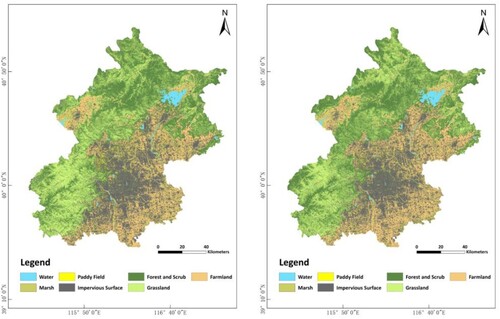
The classification results are illustrated in Figure 4. According to the statistics, the total wetland area in Beijing is 66,800 hectares in the SDGSAT-1 classification results and 41,800 hectares in the Sentinel-2 classification results. In contrast, the results of the ‘The Third National Land Survey’ in 2020 (http://ghzrzyw.beijing.gov.cn/zhengwuxinxi/sjtj/tdbgdctj/202111/t20211105_2529986.html) report the wetland area in Beijing as 62,100 hectares. Notably, the classification results of SDGSAT-1 are more consistent with the reported statistical data.

Figure 4. Wetland classification results (a), classification results based on SDGSAT-1 (b), classification results based on Sentinel-2.

To quantitatively analyze the difference in classification accuracy between the two data sources, we utilized verification samples to conduct an accuracy evaluation analysis on the classification results. The primary evaluation indicators encompass overall accuracy, Kappa coefficient, producer accuracy, user accuracy, and Macro-F1. The specific results are depicted in Figure 5.

Figure 5. The statistics of classification accuracy.

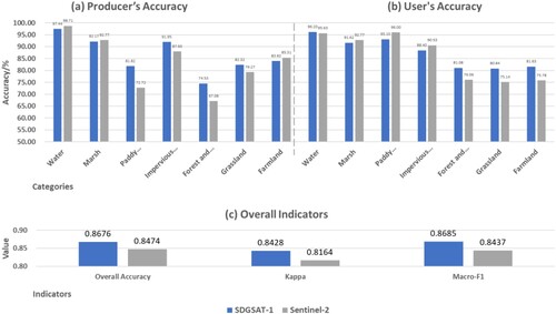
The overall accuracy of the SDGSAT-1 classification results is 86.76%, the Kappa coefficient is 0.83, and the Macro-F1 is 0.85; the overall accuracy of the Sentinel-2 classification results is 84.74%, the Kappa coefficient is 0.82, and the Macro-F1 is 0.84. In terms of the classification accuracy of individual wetland categories and overall, the accuracy of SDGSAT-1 is slightly higher than that of Sentinel-2.

The accuracy of the two classification results is approximately similar, yet the difference in wetland areas is 37%. This discrepancy arises due to the influence of the number and distribution of samples on accuracy verification, which cannot comprehensively represent the overall classification performance. Hence, qualitative analysis of specific local areas remains necessary. To address this, we conducted a comparison of the classification results in the areas of Miyun Reservoir and Guanting Reservoir, additionally incorporating existing classification products as a reference (Figure 6).

Figure 6. Comparison of classification results. The left column shows the results from Miyun Reservoir, and the right column shows the results from Guanting Reservoir.

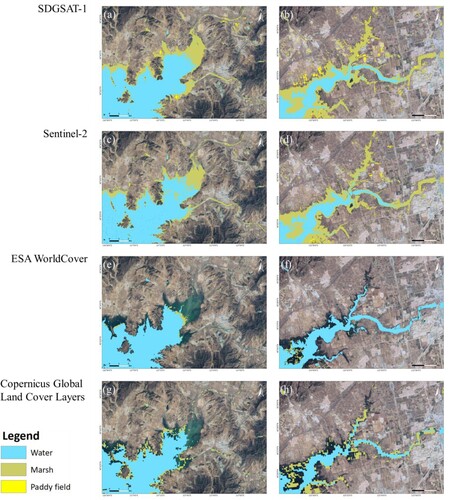
From the classification results of Miyun Reservoir and Guanting Reservoir, SDGSAT-1 data identified more marsh wetlands and paddy fields than Sentinel-2 data. The two classification products from Copernicus and ESA lack the category of paddy fields, and the area of water and marsh is also much less than the classification results in this paper. We inferred that SDGSAT-1 data is more sensitive to water information than Sentinel-2.

To further explore the impact of spectral features on classification results, we assessed the feature importance of these two classifications on Google Earth Engin (Genuer, Poggi, and Tuleau-Malot 2010). We calculated the average importance value of each feature across different months and retained the ranking results specifically for spectral features. The results are illustrated in Figure 7.

Figure 7. Importance ranking of spectral features (a), ranking the importance of the spectral features of SDGSAT-1 (b), ranking the importance of the spectral features of Sentinel-2.

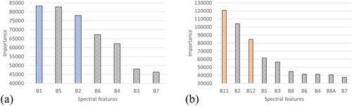
As observed, in the spectral features of SDGSAT-1, the two deep blue bands Band 1 and Band 2 are ranked first and third, respectively; whereas in the spectral features of Sentinel-2, the two short-wave infrared bands Band 11 and Band 12 are also ranked first and third, respectively. This indicates that the distinctive bands of the two satellites have a substantial impact on the classification results.

4.1.2. Exploration of SDGSAT-1’s wetland mapping capabilities

To further explore the capabilities of SDGSAT-1 in wetland mapping, we consolidated the samples into two categories: wetland and non-wetland. The JM distance between samples was computed across different spectral features of SDGSAT-1 and ranked. The results are depicted in Figure 8.

Figure 8. Ranking of sample JM distances for each spectral feature.

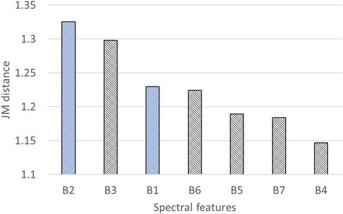
The first three bands are all blue bands, wherein Band 1 and Band 2, denoting the two deep blue bands, secure the third and first positions, respectively. The outcomes of the aforementioned experiments affirm the significant relevance of the two deep blue bands of SDGSAT-1 for wetland classification extraction.

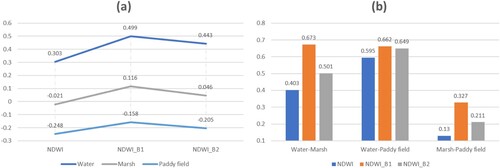
Early studies have indicated that linear or non-linear combinations of distinct spectral features can yield more effective index features (McFeeters 1996). To investigate the impact of SDGSAT-1's deep blue bands in wetland research, this study substitutes the green light band in the NDWI calculation formula with the deep blue bands, resulting in the creation of two index features, NDWI_B1 and NDWI_B2. We computed the values and variances of the three indicators – NDWI, NDWI_B1, and NDWI_B2 – across different wetland categories (Figure 9). The findings reveal that the disparities of NDWI_B1 and NDWI_B2 among diverse wetland categories surpass those of NDWI, with NDWI_B1 exhibiting the most pronounced difference. This suggests that they outperform the original NDWI index in discerning various types of wetlands.

Figure 9. (a), index values of different wetland categories (b), difference in index values of different wetland categories.

We designed two sets of experiments for comparative analysis. The first group retained the previous scheme without alterations, serving as the control group for wetland classification. In the second group, NDWI in the first group was replaced with NDWI_B1 and NDWI_B2, forming the experimental group. The experimental outcomes are illustrated in Figure 10.

Figure 10. Results of the control experiment.

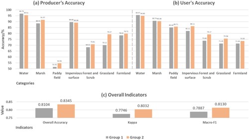
The table indicates a general trend where the classification accuracy of the experimental group surpasses that of the control group. This observation supports the effectiveness of the NDWI_B constructed using the deep blue bands in this study.

4.2. Comparison of LST retrieval results

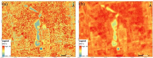
The temperature retrieval results of SDGSAT-1 and Landsat 8 are illustrated in Figure 11(a and b). Due to a two-day time difference between the acquisition of the two thermal infrared images, a direct comparison is not suitable. To address this, we normalized the temperature range of both images to the same temperature interval. Notably, an area in the Landsat 8 retrieval results appears significantly cooler than that in SDGSAT-1. Upon comparing multispectral images taken simultaneously, we identified this discrepancy as being attributed to cloud cover, as demonstrated in Figure 11(c-1 and c-2).

Figure 11. (a), the temperature retrieval result and histogram of SDGSAT-1 (b) the temperature retrieval result and histogram of Landsat 8, the red box is the area of abnormal values (c-1), the SDGSAT-1 image of the area of abnormal values (April 1) (c-2), the Landsat 8 image of the area of abnormal values (April 3).

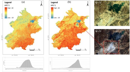
The LST retrieval results from both sensors exhibit consistency in the spatial distribution of low and high temperatures. Analysis of the histograms reveals that both datasets display an approximately skew distribution. The distinction lies in Landsat 8 having a higher kurtosis.

4.3. Comparison of wetland thermal environment analysis results

The five selected study areas in this paper are arranged from the smallest to the largest wetland area as follows: Olympic Forest Park (34.18 hm²), Beihai Park (37.51 hm²), Yuyuantan Park (41.65 hm²), Cuihu Park (137.26 hm²), and Miyun Reservoir (14632.53 hm²). Figure 12 illustrates the LST curves of the wetland buffer zones for the two retrieval results. Upon comparison, the LST curves of the SDGSAT-1 buffer zone exhibit a rough similarity to those of Landsat 8 in terms of shape and trend, yet the SDGSAT-1 curves demonstrate more pronounced fluctuations.

Figure 12. LST curves of the buffer zones of the five wetlands, with red dots representing turning points (a), LST curve of retrieval results of SDGSAT-1 (b), LST curve of retrieval results of Landsat 8.

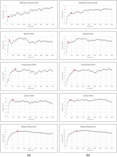
The outcomes derived from the LST curve analysis are presented in Table 6. With the exception of Olympic Forest Park, the breakpoint distance, cooling intensity, and temperature gradient of SDGSAT-1 and Landsat 8 exhibit relatively close values in the remaining experimental areas. Both sets of statistical results indicate a positive correlation between breakpoint distance, cooling intensity, and wetland area, aligning with findings from previous research.

Table 6. LST characteristic statistics of wetland buffer zone.

Satellite	Wetland Name	Wetland area (km²)	Wetland temperature (°C)	Turning temperature (°C)	Turning distance (m)	Temperature difference (°C)	Temperature gradient (°C/km)
SDGSAT-1	Olympic Forest Park	0.34	12.68	17.12	150	4.44	29.62
	Beihai Park	0.38	11.92	20.16	200	8.24	41.19
	Yuyuantan Park	0.42	12.29	20.52	750	8.23	10.97
	Cuihu Park	1.37	13.02	18.85	450	5.84	12.97
	Miyun Reservoir	146.33	6.58	18.32	950	11.74	12.37
Landsat 8	Olympic Forest Park	0.34	17.68	22.87	450	5.19	11.52
	Beihai Park	0.37	15.35	24.55	200	9.20	45.99
	Yuyuantan Park	0.42	15.48	24.84	750	9.37	12.49
	Cuihu Park	1.34	17.82	24.56	400	6.74	16.84
	Miyun Reservoir	159.15	3.17	21.10	950	17.93	18.87

5. Discussion

5.1. The ability of SDGSAT-1 data in wetland information extraction

Various factors influence the precision of wetland classification, including samples, classification features, resolution, and classification algorithms. In this study, we controlled other variables, focusing solely on comparing the impact of different spectral features on classification. The results indicate that SDGSAT-1 exhibits superior wetland classification ability compared to Sentinel-2. This enhancement is attributed, in part, to the inclusion of its deep blue bands, specifically Band 1 and Band 2. In recent years, Sentinel-2 data has been widely employed for wetland and water body extraction, yielding commendable results (Filippucci et al. 2022; Schwatke, Scherer, and Dettmering 2019; Yang Li and Niu 2022). Sentinel-2's high spatial and temporal resolution, coupled with the effectiveness of the Modified Normalized Difference Water Index (MNDWI) calculated using short-wave infrared and green light bands, contribute to its success (H. Xu 2006). While SDGSAT-1 lacks a short-wave infrared band for MNDWI calculation, its potential is demonstrated through linear or nonlinear combinations of different bands, yielding new indices that provide effective information. In this study, a simple substitution of the green light band with the deep blue band to construct NDWI_B proved effective in wetland classification. While constructing index features demands rigorous experimental design, the primary focus of this paper is not on optimizing index features but on showcasing the potential of deep blue bands in wetland research, laying the groundwork for future investigations. Thus, we anticipate that future research will explore the utilization of SDGSAT-1's deep blue band in combination with other bands to construct new index features.

5.2. Advantages and disadvantages of SDGSAT-1 thermal infrared data

In prior research on wetland thermal environments, interpolation data from ground measurement sites (Yang, Xiao, and Ye 2016) or thermal infrared data with lower spatial resolutions, such as Landsat, ASTER, or MODIS (Cao et al. 2010; Wang and Zhu 2011) were commonly utilized for analyzing the spatial variation of surface temperature. The scale of analysis typically ranged in units of hundreds or several hundred meters. In the comparative experiment conducted in this paper, it was observed that in areas where the Landsat 8 temperature curve exhibited relative flatness, the SDGSAT-1 temperature curve displayed significant fluctuations, effectively capturing temperature changes around the wetland within a small range. Using the area around the Forbidden City as an example, as illustrated in Figure 13, the LST retrieval results from SDGSAT-1 distinctly outline the Jinshui River surrounding the entire Forbidden City and Sanhai on the west side. The edges are sharply defined, and roads and building shadows are discernible to the naked eye. The patches appear relatively fragmented, showcasing temperature differences within a small range. In contrast, the retrieval results from Landsat 8 only manage to delineate the general outline of Sanhai, with roads and buildings remaining indistinguishable in the image. The patches exhibit a smoother texture and only convey the general distribution of temperature in space, lacking the ability to reflect small-scale temperature changes. Therefore, SDGSAT-1 lays a solid data foundation for more detailed research on wetland thermal environments or the urban heat island effect.

Figure 13. LST retrieval results of the area around the Forbidden City (a), the result of SDGSAT-1 (b), the result of Landsat 8.

6. Main conclusions

The recently launched SDGSAT-1 in 2021 represents a significant advancement, equipped with multiple sensors and boasting a high resolution of 10 m. This satellite emerges as a cutting-edge technological tool for investigating human activities and urban natural environments. Through a comparative research approach utilizing Sentinel 2 and Landsat 8 OLI data, we assess the capabilities of SDGSAT-1 data in monitoring human activities and the natural environment, focusing on Beijing as the research area. Our findings lead to the following conclusions:

1. The monitoring performance of urban wetlands using SDGSAT-1 data surpasses that of Sentinel-2 satellite data. Wetland classification based on SDGSAT-1 data achieves an overall accuracy of 86.76%, a Kappa coefficient of 0.84, and a Macro-F1 of 0.87. Subsequent analysis indicates that the deep blue bands spanning 374–427 nm and 410–467 nm play a crucial role in enhancing the capability of wetland classification.

2. The capabilities of SDGSAT-1 satellite data in capturing the relationship between urban wetlands and the land thermal environment surpass those of Landsat OLI. This improvement can be attributed to the higher spatial resolution of the thermal infrared band (30 m) in SDGSAT-1, enabling the easy identification of many small wetlands.

3. SDGSAT-1 data has demonstrated significant and comprehensive advantages in monitoring urban wetlands and the thermal environment. If the production department continues to deliver high-quality data consistently, it will contribute significantly to the management and development of urban wetlands.

Acknowledgements

We gratefully thank the International Research Center of Big Data for Sustainable Development Goals for providing SDGSAT-1 data. This research was supported by the international services and collaborative applications of global remote sensing data and products for typical land covers at 10 m scale using domestic satellite data (2021YFE0194700), the Strategic Priority Research Program of the Chinese Academy of Sciences (XDA19030203), the National Natural Science Foundation of China (41971390).

Data availability statement

The data that support the findings of this study are openly available in Science Data Bank at http://10.57760/sciencedb.09873.

Disclosure statement

No potential conflict of interest was reported by the author(s).

Additional information

Funding

This work was supported by State Key Laboratory of Remote Sensing Science [grant number 2021YFE0194700, XDA19030203, 41971390].

References

- Aboelata, Amir. 2020. “Vegetation in Different Street Orientations of Aspect Ratio (H/W 1: 1) to Mitigate UHI and Reduce Buildings’ Energy in Arid Climate.” Building and Environment 172, Elsevier: 106712. https://doi.org/10.1016/j.buildenv.2020.106712.
- Alikhani, Somayeh, Petri Nummi, and Anne Ojala. 2021. “Urban Wetlands: A Review on Ecological and Cultural Values.” Water 13 (22) Multidisciplinary Digital Publishing Institute: 3301. https://doi.org/10.3390/w13223301.
- Bajaj, Divya N., Arun B. Inamdar, and Vineet Vaibhav. 2012. “Temporal Variation of Urban Heat Island Using Landsat Data: A Case Study of Ahmedabad, India.” In 33rd Asian Conference on Remote Sensing 2012, ACRS-2012, 797–804. Asian Association on Remote Sensing.
- Broge, Niels Henrik., and Eric Leblanc. 2001. “Comparing Prediction Power and Stability of Broadband and Hyperspectral Vegetation Indices for Estimation of Green Leaf Area Index and Canopy Chlorophyll Density.” Remote Sensing of Environment 76 (2): 156–172. https://doi.org/10.1016/S0034-4257(00)00197-8.
- Buchhorn, Marcel, Myroslava Lesiv, Nandin-Erdene Tsendbazar, Martin Herold, Luc Bertels, and Bruno Smets. 2020. “Copernicus Global Land Cover Layers—Collection 2.” Remote Sensing 12 (6) MDPI: 1044. https://doi.org/10.3390/rs12061044.
- Buyantuyev, Alexander, and Jianguo Wu. 2010. “Urban Heat Islands and Landscape Heterogeneity: Linking Spatiotemporal Variations in Surface Temperatures to Land-Cover and Socioeconomic Patterns.” Landscape Ecology 25 (1) Springer: 17–33. https://doi.org/10.1007/s10980-009-9402-4.
- Cao, Xin, Akio Onishi, Jin Chen, and Hidefumi Imura. 2010. “Quantifying the Cool Island Intensity of Urban Parks Using ASTER and IKONOS Data.” Landscape and Urban Planning 96 (4) Elsevier: 224–231. https://doi.org/10.1016/j.landurbplan.2010.03.008.
- Chang, Chiru, Minghuang Li, and Shyhdean Chang. 2007. “A Preliminary Study on the Local Cool-Island Intensity of Taipei City Parks.” Landscape and Urban Planning 80 (4) Elsevier: 386–395. https://doi.org/10.1016/j.landurbplan.2006.09.005.
- Chen, Yanfen., Zhenguo Niu, Shengjie Hu, and Haiying Zhang. 2016. “Dynamic Monitoring of Dongting Lake Wetland Using Time-series MODIS Imagery.” Journal of Hydraulic Engineering 47 (9): 1093–1104.
- Clinton, Nicholas, and Peng Gong. 2013. “MODIS Detected Surface Urban Heat Islands and Sinks: Global Locations and Controls.” Remote Sensing of Environment 134, Elsevier: 294–304. https://doi.org/10.1016/j.rse.2013.03.008.
- Dabboor, M., S. Howell, M. Shokr, and J. Yackel. 2014. “The Jeffries–Matusita Distance for the Case of Complex Wishart Distribution as a Separability Criterion for Fully Polarimetric SAR Data.” International Journal of Remote Sensing 35 (19) Taylor & Francis: 6859–6873.
- Du, Hongyu, Xuejun Song, Hong Jiang, Zenghui Kan, Zhibao Wang, and Yongli Cai. 2016. “Research on the Cooling Island Effects of Water Body: A Case Study of Shanghai, China.” Ecological Indicators 67, Elsevier: 31–38. https://doi.org/10.1016/j.ecolind.2016.02.040.
- Farr, Tom G., Paul A. Rosen, Edward Caro, Robert Crippen, Riley Duren, Scott Hensley, Michael Kobrick, Mimi Paller, Ernesto Rodriguez, and Ladislav Roth. 2007. “The Shuttle Radar Topography Mission.” Reviews of Geophysics 45 (2). https://doi.org/10.1029/2005RG000183.
- Filippucci, Paolo, Luca Brocca, Stefania Bonafoni, Carla Saltalippi, Wolfgang Wagner, and Angelica Tarpanelli. 2022. “Sentinel-2 High-Resolution Data for River Discharge Monitoring.” Remote Sensing of Environment 281 (November). https://doi.org/10.1016/j.rse.2022.113255.
- Freund, Yoav, Robert Schapire, and Naoki Abe. 1999. “A Short Introduction to Boosting.” Journal-Japanese Society For Artificial Intelligence 14 (771–780): 1612.
- Friedman, Jerome H. 2001. “Greedy Function Approximation: A Gradient Boosting Machine.” Annals of Statistics 29 (5): 1189–1232. https://doi.org/10.1214/aos/1013203451.
- Fu, Bolin, Sunzhe Li, Zhinan Lao, Bingyan Yuan, Yiyin Liang, Wen He, Weiwei Sun, and Hongchang He. 2023. “Multi-sensor and Multi-Platform Retrieval of Water Chlorophyll a Concentration in Karst Wetlands Using Transfer Learning Frameworks with ASD, UAV, and Planet CubeSate Reflectance Data.” Science of The Total Environment 901 (November): 165963. https://doi.org/10.1016/j.scitotenv.2023.165963.
- Garcia Salgado, Beatriz Paulina, and Volodymyr Ponomaryov. 2015. “Feature Extraction-Selection Scheme for Hyperspectral Image Classification Using Fourier Transform and Jeffries-Matusita Distance.” In Advances in Artificial Intelligence and Its Applications: 14th Mexican International Conference on Artificial Intelligence, MICAI 2015, Cuernavaca, Morelos, Mexico, October 25-31, 2015, Proceedings, Part II 14, 337–348. Springer.
- Genuer, Robin, Jean Michel Poggi, and Christine Tuleau Malot. 2010. “Variable Selection Using Random Forests.” Pattern Recognition Letters 31 (14) Elsevier: 2225–2236. https://doi.org/10.1016/j.patrec.2010.03.014.
- Gorelick, Noel, Matt Hancher, Mike Dixon, Simon Ilyushchenko, David Thau, and Rebecca Moore. 2017. “Google Earth Engine: Planetary-scale Geospatial Analysis for Everyone.” Remote Sensing of Environment, Big Remotely Sensed Data: tools, applications and experiences 202 (December): 18–27. https://doi.org/10.1016/j.rse.2017.06.031.
- Guo, Huadong, Changyong Dou, Hongyu Chen, Jianbo Liu, Bihong Fu, Xiaoming Li, Ziming Zou, and Dong Liang. 2023. “SDGSAT-1: The World’s First Scientific Satellite for Sustainable Development Goals.” Science Bulletin 68 (1): 34–38. https://doi.org/10.1016/j.scib.2022.12.014.
- Haboudane, Driss, John R. Miller, Nicolas Tremblay, Pablo J. Zarco-Tejada, and Louise Dextraze. 2002. “Integrated Narrow-Band Vegetation Indices for Prediction of Crop Chlorophyll Content for Application to Precision Agriculture.” Remote Sensing of Environment 81 (2–3): 416–426. https://doi.org/10.1016/S0034-4257(02)00018-4.
- He, Bao-Jie, Junsong Wang, Huimin Liu, and Giulia Ulpiani. 2021. “Localized Synergies between Heat Waves and Urban Heat Islands: Implications on Human Thermal Comfort and Urban Heat Management.” Environmental Research 193, Elsevier: 110584. https://doi.org/10.1016/j.envres.2020.110584.
- Huang, Yi, Jiangtao Peng, Na Chen, Weiwei Sun, Qian Du, Kai Ren, and Ke Huang. 2023. “Cross-scene Wetland Mapping on Hyperspectral Remote Sensing Images Using Adversarial Domain Adaptation Network.” ISPRS Journal of Photogrammetry and Remote Sensing 203 (September): 37–54. https://doi.org/10.1016/j.isprsjprs.2023.07.009.
- Huete, A. R. 1988. “A Soil-adjusted Vegetation Index (SAVI).” Remote Sensing of Environment 25 (3): 295–309. https://doi.org/10.1016/0034-4257(88)90106-X.
- Huete, A., K. Didan, T. Miura, E. P. Rodriguez, X. Gao, and L. G. Ferreira. 2002. “Overview of the Radiometric and Biophysical Performance of the MODIS Vegetation Indices.” Remote Sensing of Environment, The Moderate Resolution Imaging Spectroradiometer (MODIS): a new generation of Land Surface Monitoring 83 (1–2): 195–213. https://doi.org/10.1016/S0034-4257(02)00096-2.
- Kuang, Wenhui, Yue Liu, Yinyin Dou, Wenfeng Chi, Guangsheng Chen, Chengfeng Gao, Tianrong Yang, Jiyuan Liu, and Renhua Zhang. 2015. “What are Hot and What are Not in an Urban Landscape: Quantifying and Explaining the Land Surface Temperature Pattern in Beijing, China.” Landscape Ecology 30 (2) Springer: 357–373. https://doi.org/10.1007/s10980-014-0128-6.
- Lazzarini, Michele, Prashanth Reddy Marpu, and Hosni Ghedira. 2013. “Temperature-land Cover Interactions: The Inversion of Urban Heat Island Phenomenon in Desert City Areas.” Remote Sensing of Environment 130, Elsevier: 136–152. https://doi.org/10.1016/j.rse.2012.11.007.
- Lee, Hyoun-Young. 1993. “An Application of NOAA AVHRR Thermal Data to the Study of Urban Heat Islands.” Atmospheric Environment. Part B. Urban Atmosphere 27 (1) Elsevier: 1–13. https://doi.org/10.1016/0957-1272(93)90041-4.
- Li, Miaomiao. 2003. The Method of Vegetation Fraction Estimation by Remote Sensing. Beijing: Chinese Academy of Sciences.
- Li, Yang, and Zhenguo Niu. 2022. “Systematic Method for Mapping Fine-resolution Water Cover Types in China Based on Time Series Sentinel-1 and 2 Images.” International Journal of Applied Earth Observation and Geoinformation 106, Elsevier: 102656. https://doi.org/10.1016/j.jag.2021.102656.
- Li, Tong, Ying Xu, and Lei Yao. 2021. “Detecting Urban Landscape Factors Controlling Seasonal Land Surface Temperature: From the Perspective of Urban Function Zones.” Environmental Science and Pollution Research 28 (30): 41191–41206. https://doi.org/10.1007/s11356-021-13695-y.
- Li, Yingying, Hao Zhang, and Wolfgang Kainz. 2012. “Monitoring Patterns of Urban Heat Islands of the Fast-Growing Shanghai Metropolis, China: Using Time-Series of Landsat TM/ETM+ Data.” International Journal of Applied Earth Observation and Geoinformation 19, Elsevier: 127–138. https://doi.org/10.1016/j.jag.2012.05.001.
- Liu, Kai, Weiwei Sun, Yijun Shao, Weiwei Liu, Gang Yang, Xiangchao Meng, Jiangtao Peng, Dehua Mao, and Kai Ren. 2022. “Mapping Coastal Wetlands Using Transformer in Transformer Deep Network on China ZY1-02D Hyperspectral Satellite Images.” IEEE Journal of Selected Topics in Applied Earth Observations and Remote Sensing 15:3891–3903. https://doi.org/10.1109/JSTARS.2022.3173349.
- Lo, Chor Pang, Dale A. Quattrochi, and Jeffrey C. Luvall. 1997. “Application of High-resolution Thermal Infrared Remote Sensing and GIS to Assess the Urban Heat Island Effect.” International Journal of Remote Sensing 18 (2) Taylor & Francis: 287–304. https://doi.org/10.1080/014311697219079.
- Manteghi, Golnoosh, Hasanuddin Lamit, and Dilshan Ossen. 2015. “Water Bodies an Urban Microclimate: A Review.” Modern Applied Science 9 (February). https://doi.org/10.5539/mas.v9n6p1.
- McFeeters, Stuart K. 1996. “The Use of the Normalized Difference Water Index (NDWI) in the Delineation of Open Water Features.” International Journal of Remote Sensing 17 (7) Taylor & Francis: 1425–1432. https://doi.org/10.1080/01431169608948714.
- Niu, ZhenGuo, Peng Gong, Xiao Cheng, JianHong Guo, Lin Wang, HuaBing Huang, ShaoQing Shen, et al. 2009. “Geographical Characteristics of China’s Wetlands Derived from Remotely Sensed Data.” Science in China Series D: Earth Sciences 52 (6) Springer: 723–738. https://doi.org/10.1007/s11430-009-0075-2.
- Nowakowski, Artur. 2015. “Remote Sensing Data Binary Classification Using Boosting with Simple Classifiers.” Acta Geophysica 63 (5) Springer: 1447–1462. https://doi.org/10.1515/acgeo-2015-0040.
- Oke, Tim R. 1973. “City Size and the Urban Heat Island.” Atmospheric Environment (1967) 7 (8) Elsevier: 769–779. https://doi.org/10.1016/0004-6981(73)90140-6.
- Rao, B. R. M., R. S. Dwivedi, S. P. S. Kushwaha, S. N. Bhattacharya, J. B. Anand, and S. Dasgupta. 1999. “Monitoring the Spatial Extent of Coastal Wetlands Using ERS-1 SAR Data.” International Journal of Remote Sensing 20 (13) Taylor & Francis: 2509–2517. https://doi.org/10.1080/014311699211903.
- Rasul, Azad, Heiko Balzter, Claire Smith, John Remedios, Bashir Adamu, José A. Sobrino, Manat Srivanit, and Qihao Weng. 2017. “A Review on Remote Sensing of Urban Heat and Cool Islands.” Land 6 (2) MDPI: 38. https://doi.org/10.3390/land6020038.
- Roujean, Jean-Louis, and François-Marie Breon. 1995. “Estimating PAR Absorbed by Vegetation from Bidirectional Reflectance Measurements.” Remote Sensing of Environment 51 (3): 375–384. https://doi.org/10.1016/0034-4257(94)00114-3.
- Rouse, John Wilson, Rüdiger H. Haas, John A. Schell, and Donald W. Deering. 1974. “Monitoring Vegetation Systems in the Great Plains with ERTS.” NASA Special Publications 351 (1): 309.
- Schwatke, Christian, Daniel Scherer, and Denise Dettmering. 2019. “Automated Extraction of Consistent Time-Variable Water Surfaces of Lakes and Reservoirs Based on Landsat and Sentinel-2.” Remote Sensing 11 (9) Multidisciplinary Digital Publishing Institute: 1010. https://doi.org/10.3390/rs11091010.
- Sen, Rikta, Saptarsi Goswami, and Basabi Chakraborty. 2019. “Jeffries-Matusita Distance as a Tool for Feature Selection.” In 2019 International Conference on Data Science and Engineering (ICDSE), 15–20. IEEE.
- Sobrino, José A., Juan C. Jiménez-Muñoz, and Leonardo Paolini. 2004. “Land Surface Temperature Retrieval from LANDSAT TM 5.” Remote Sensing of Environment 90 (4): 434–440. https://doi.org/10.1016/j.rse.2004.02.003.
- Streutker, David R. 2002. “A Remote Sensing Study of the Urban Heat Island of Houston, Texas.” International Journal of Remote Sensing 23 (13) Taylor & Francis: 2595–2608. https://doi.org/10.1080/01431160110115023.
- Sun, Renhao, Ailian Chen, Liding Chen, and Yihe Lü. 2012. “Cooling Effects of Wetlands in an Urban Region: The Case of Beijing.” Ecological Indicators 20, Elsevier: 57–64. https://doi.org/10.1016/j.ecolind.2012.02.006.
- Sun, Weiwei, Kai Ren, Xiangchao Meng, Gang Yang, Jiangtao Peng, and Jiancheng Li. 2023. “Unsupervised 3-D Tensor Subspace Decomposition Network for Spatial–Temporal–Spectral Fusion of Hyperspectral and Multispectral Images.” IEEE Transactions on Geoscience and Remote Sensing 61:1–17. https://doi.org/10.1109/TGRS.2023.3324028.
- Voogt, James A., and Tim R. Oke. 2003. “Thermal Remote Sensing of Urban Climates.” Remote Sensing of Environment 86 (3) Elsevier: 370–384. https://doi.org/10.1016/S0034-4257(03)00079-8.
- Wang, Chunye, and Weiping Zhu. 2011. “Analysis of the Impact of Urban Wetland on Urban Temperature Based on Remote Sensing Technology.” Procedia Environmental Sciences 10, Elsevier: 1546–1552. https://doi.org/10.1016/j.proenv.2011.09.246.
- Xing, Liwei, and Zhenguo Niu. 2019. “Mapping and Analyzing China’s Wetlands Using MODIS Time Series Data.” Wetlands Ecology and Management 27 (5–6) Springer: 693–710. https://doi.org/10.1007/s11273-019-09687-y.
- Xu, Hanqiu. 2006. “Modification of Normalised Difference Water Index (NDWI) to Enhance Open Water Features in Remotely Sensed Imagery.” International Journal of Remote Sensing 27 (14) Taylor & Francis: 3025–3033. https://doi.org/10.1080/01431160600589179.
- Xu, Yongming, Zhihao Qin, and Jingjing Lv. 2008. “Comparative Analysis of Urban Heat Island and Associated Land Cover Change Based in Suzhou City Using Landsat Data.” In 2008 International Workshop on Education Technology and Training & 2008 International Workshop on Geoscience and Remote Sensing, Vol. 2, 316–319. IEEE.
- Yang, Chenghai, James H. Everitt, Joe M. Bradford, and Dale Murden. 2004. “Airborne Hyperspectral Imagery and Yield Monitor Data for Mapping Cotton Yield Variability.” Precision Agriculture 5 (5): 445–461. https://doi.org/10.1007/s11119-004-5319-8.
- Yang, Xiao, Sen Liu, Chao Jia, Yang Liu, and Cuicui Yu. 2021. “Vulnerability Assessment and Management Planning for the Ecological Environment in Urban Wetlands.” Journal of Environmental Management 298 (November): 113540. https://doi.org/10.1016/j.jenvman.2021.113540.
- Yang, Ping, Ziniu Xiao, and Mengshu Ye. 2016. “Cooling Effect of Urban Parks and their Relationship with Urban Heat Islands.” Atmospheric and Oceanic Science Letters 9 (4) Taylor & Francis: 298–305. https://doi.org/10.1080/16742834.2016.1191316.
- Yao, Lei, Ying Xu, and Baolei Zhang. 2019. “Effect of Urban Function and Landscape Structure on the Urban Heat Island Phenomenon in Beijing, China.” Landscape and Ecological Engineering 15 (4): 379–390. https://doi.org/10.1007/s11355-019-00388-5.
- Yin, Xiaolan, Chengyue Tan, Yinghai Ke, and Demin Zhou. 2024. “Evolution and Driving Factors of Salt Marsh Wetland Landscape Pattern in the Yellow River Delta during 1973—2020.” Acta Ecologica Sinica. https://www.ecologica.cn//stxb/article/abstract/stxb202211203355.
- Zanaga, Daniele, Ruben Van De Kerchove, Dirk Daems, Wanda De Keersmaecker, Carsten Brockmann, Grit Kirches, Jan Wevers, et al. 2022. “ESA WorldCover 10 m 2021 V200.” Zenodo. https://doi.org/10.5281/zenodo.7254221.
- Zhang, Bo, Zhenguo Niu, Dongqi Zhang, and Xuanlin Huo. 2022. “Dynamic Changes and Driving Forces of Alpine Wetlands on the Qinghai–Tibetan Plateau Based on Long-Term Time Series Satellite Data: A Case Study in the Gansu Maqu Wetlands.” Remote Sensing 14 (17) MDPI: 4147. https://doi.org/10.3390/rs14174147.
- Zhong, Liheng, Lina Hu, and Hang Zhou. 2019. “Deep Learning Based Multi-Temporal Crop Classification.” Remote Sensing of Environment 221, Elsevier: 430–443. https://doi.org/10.1016/j.rse.2018.11.032.
- Zhou, Huiping, Hong Jiang, Guomo Zhou, Xiaodong Song, Shuquan Yu, Jie Chang, Shirong Liu, Zishan Jiang, and Bo Jiang. 2010. “Monitoring the Change of Urban Wetland Using High Spatial Resolution Remote Sensing Data.” International Journal of Remote Sensing 31 (7) Taylor & Francis: 1717–1731. https://doi.org/10.1080/01431160902926608.