Forest above-ground biomass estimation using X, C, L, and P band SAR polarimetric observations and different inversion models

ABSTRACT

Since each frequency senses distinct features of forest structure, it is attractive to understand whether complementarity of multi-frequency can improve the retrieval of forest above ground biomass (AGB). In this study, 15 combinations of X, C, L, and P band SAR observations were applied in the forest AGB estimation through multivariate linear stepwise regression (MLSR), random forest (RF), and deep learning algorithm based on Keras and TensorFlow algorithms to fully explore their potential and capability for forest AGB retrieval. 21 SAR observations were derived from each frequency and worked as SAR observations for forest AGB estimation. According to the retrieval results using three inversion algorithms and 15 SAR observation combinations, MLSR algorithm with combined L and P band SAR observations performed best with R² = 0.67 and RMSE = 14.51 Mg/ha. Next was RF algorithm with combination of L and P band, the R² and RMSE are 0.64 and15.20 Mg/ha, respectively. L and P band are more suitable frequencies for estimating forest AGB, only limited improvements can be achieved by combing them with X and C band. Combination of L and P band can obtain comparable AGB estimation accuracy with using combinations from tri- or quad-frequency SAR observations.

KEYWORDS:

• Forest AGB
• multi-frequency SAR observables
• MLSR
• RF
• a deep learning algorithm

1. Introduction

It is universally recognized that forests play an important role in the main terrestrial carbon sink. Forest living above-ground biomass (AGB), i.e. the dry weight of trees per unit area excluding roots, shrubs, herbs and rotten leaves under the forest, makes a significant contribution to the carbon reservoir, which is related to the global carbon cycle and ultimately fed back to climate (Cartus et al. 2019; Santi et al. 2017; Santoro et al. 2019). The most precise method of obtaining forest AGB data is destructive sampling, which involves gathering, drying, and weighing living biomass. However, the destructive method is costly, time-consuming, limited in regions with scarce accessibility, and is difficult to obtain wall-to-wall spatial and temporal dynamics of AGB information (Englhart, Keuck, and Siegert 2011; Goetz et al. 2009; Malhi et al. 2004). Considering the disadvantages of the destructive method for AGB estimation, previous published literature demonstrated the capability and advantages of remote sensing observations for forest AGB estimation (Englhart, Keuck, and Siegert 2011; Lu 2006; Lu et al. 2016). It has been determined that synthetic aperture radar (SAR) data, which benefit from their independence from cloud cover and weather conditions as well as their great penetration through the vegetation, are a more acceptable method for estimating forest AGB (Le Toan et al. 2001; Santi et al. 2017; Zeng et al. 2022).

Since forest AGB cannot be directly measured by remote sensing observations, the signal recorded by SAR in the forest-covered area is strongly affected by moisture content related to the water content of the tree and geometrical features including tree architecture (e.g. leaves, branches, and trunks) and the arrangement of trees on the ground (Englhart, Keuck, and Siegert 2011; Rosenqvist et al. 2003; Santoro et al. 2019). Depending on the frequency and polarization of the radar being used, these factors have different effects on scattering (Ferrazzoli and Guerriero 1995; Santi et al. 2017). According to the scattering theories, each wavelength and polarization detects a different aspect of the structure of the forest (Cartus and Santoro 2019). At high frequencies with operated wavelengths shorter than 10 cm (X and C bands), the signal originates primarily from small tree aspects such as leaves or needles, foliage, and small branches of the first layer of canopy. For longer wavelengths, i.e. L and P bands, the signal is mainly scattered from primary branches and trunks, whereas the contribution of twigs and leaves is negligible (Santi et al. 2017; Santoro et al. 2019). Radar polarimetry characterizes information on geometrical structures such as shape, orientation, and geophysical characteristics of the object are dealing with the complete vector nature of polarized electromagnetic waves (Chowdhury et al. 2013). Previous studies showed that backscatter coefficients at various frequencies and polarizations were sensitive to forest characteristics and then allowed a good performance for forest area identification and forest parameters inversion. However, several studies also stated that the backscatter saturation of each frequency in the forest AGB inversion (Imhoff 1995; Le Toan et al. 1992; 2011; Santi et al. 2017).

The exploration of multi-frequency techniques for estimating forest AGB has been driven by the limitation of each single frequency to estimate forest AGB up to the saturation threshold (Cartus et al. 2019; Englhart, Keuck, and Siegert 2011; Harrell et al. 1995; Imhoff 1995; Kurvonen, Pulliainen, and Hallikainen 1999; Ranson and Sun 1994; Santi et al. 2017; Santoro et al. 2019). The earliest research on forest AGB retrieval using multi-frequency observations was reported in the 1990s, the studies focused on a combination of C, L, and P band backscatter coefficients to estimate forest AGB and confirmed that the use of multi-frequency SAR observations allowed for improved forest AGB estimation accuracies (Harrell et al. 1995; Imhoff 1995; Kurvonen, Pulliainen, and Hallikainen 1999; Ranson and Sun 1994). Englhart, Keuck, and Siegert (2011) reported that combined L and X bands showed an obvious improvement in performance in forest AGB estimation compared with the performance of each single frequency. Cartus et al. (2019) investigated the combination of C, L, and P band backscatter coefficients for a boreal forest AGB estimation and concluded that the combination of multi-temporal C and L band observations achieved comparable accuracies as single P band observations. Cartus et al. (2019) investigated the feasibility of using multi-temporal and multi-frequency SAR backscatter measurements to estimate AGB in tropical forests and confirmed that the P band is the best frequency for retrieving AGB in the tropics. They also concluded that the use of multi-temporal observations is beneficial to each frequency and the combination of tri-frequency SAR backscatter observations did not improve retrieval performance of the combination of dual-frequency observations. In the study of Saatchi et al. (2007), the combined P and L band observations did not improve the forest AGB retrieval accuracy compared with the performance of a single P band.

Algorithms applied in forest AGB inversion can be grouped into parametric and nonparametric ones. Parametric algorithms like simple or multiple linear regression models assume the relationship between forest AGB and remote sensing observations have explicit model structures and it can be specified a priori by parameters (Lu et al. 2016). Regression-based models with the advantage of flexibility and high interpretability have been useful in forest AGB estimation (Gonçalves, Santos, and Treuhaft 2011; He et al. 2013; Tsui et al. 2012; Zeng et al. 2022). SAR and LiDAR observations using parametric models showed good performance in forest AGB inversion of different tree species (Li et al. 2023; Zeng et al. 2022). However, in reality, parametric algorithms usually struggle to handle the intricate interactions between AGB and remote sensing variables. Nonparametric algorithms determined that the model structure in a data-driven manner is more flexible and efficient for solving the nonlinear relationships between forest AGB and remote sensing observations. Nonparametric algorithms including K-nearest neighbor (KNN), artificial neural network (ANN), random forest (RF), support vector regression (SVR), and Maximum Entropy (MaxEnt) were applied in forest AGB inversion using remote sensing measurements in previous studies (Foody, Boyd, and Cutler 2003; Lu et al. 2016; Saatchi et al. 2011; Zhang et al. 2022). The RF algorithm demonstrated good performance in predicting vegetation attributes with remote sensing measurements (Guerra-Hernández et al. 2022; Nandy, Srinet, and Padalia 2021; Wang et al. 2019). Previous studies demonstrated that it provided robust retrieval results for different vegetation attributes. They also stated the overestimation of ANN and KNN algorithms (Wang et al. 2019; Zhang et al. 2022).

With the abundance of polarimetric information extraction methods, several polarimetric SAR observations were extracted and could be used for forest AGB estimation. Previous research found that selecting acceptable remote sensing observations and inversion modeling algorithms are crucial steps in the forest AGB inversion procedure using remote sensing technology (Gao et al. 2018; Lu et al. 2016). Both parametric algorithms like (multivariate linear step regression) MLSR and nonparametric algorithms like RF can select suitable SAR features and estimate forest AGBs. Due to its simplification and comparatively strong performance, MLSR has been extensively utilized for estimating forest AGB. However, because it relies on a linear relationship between AGB and remote sensing observations, it might not produce adequate results because AGB and remote sensing features have a complex non-linear relationship (Englhart, Keuck, and Siegert 2011; Lu et al. 2016). Since RF can handle large amounts of data quickly and efficiently, handle nonlinear relationships between remote sensing observations and AGB, and also rank the significance of input remote sensing features, it can increase estimation accuracy (Breiman 2001; Gao et al. 2018; Lu et al. 2016; Wang et al. 2019).

The theory of deep learning was proposed by Hinton et al. in 2008, then it has been widely used in image classification, target detection, and semantic segmentation. Deep learning was developed as a subfield of machine learning algorithms and can also interpret nonlinear patterns in data by mimicking the neural architecture of the human brain (Beysolow 2017; Hinton et al. 2008). Compared with traditional machine learning methods, the advantage of deep learning is that effective features can be automatically extracted from all the features of the original image to participate in the calculation, thus avoiding the strong subjectivity caused by human feature selection in the early stage and making full use of the rich spectral features, spatial features and other related information to reduce the impact of the homogeneous and heterogeneous phenomena. Deep learning models have been used in forest AGB estimation recently. Zhang et al. (2019) applied the Stacked Sparse Autoencoder network algorithm in forest AGB estimation and found it outperformed RF and SVR. However, Deep learning models have not been fully explored in forest AGB estimation. Keras using Tensorflow as a back end is the most popular and widely used framework and it is written in Python and can be used in R interface with a few lines of code (Ghosh and Behera 2021).

Since previous investigations of multi-frequency applications in forest AGB estimation were exploratory, there are still a lot of research gaps relating to the actual potential of using multi-frequency observations, especially polarimetric multi-frequency observations to improve the accuracy of forest AGB estimation. For instance, Does the joint use of more frequencies allow for more improvement of the forest AGB retrieval? The combination of which frequencies performed best in forest AGB retrieval? Whether the retrieval algorithms affect the performance of forest AGB retrieval when using multi-frequency SAR observation? Whether adding polarimetric information in multi-frequency SAR observations allow for improving retrieval accuracy? To answer these questions, a typical cold temperate coniferous mixed forest in Northeast China is taken as the study area, X, C, L and P band quad-polarimetric multi-frequency SAR data and a parametric like MLSR, a nonparametric retrieval algorithm of RF, and a deep learning algorithm of Keras based on Tensorflow were used in the study to explore the potential of combinations of multi-frequency polarimetric SAR observations for forest AGB retrieval.

2. Materials

2.1. Test site

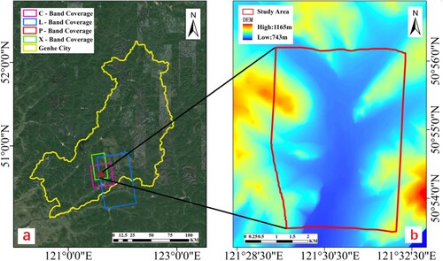
The test site is in Genhe Ecological Station, Genhe City (50°20′ to 52°30′ N, 120°12′ to 122°55′ E; Figure 1(a)), the north-east of Hulunbuir League, Inner Mongolia, north-east of China. The elevation within the test site varies from 700 to 1200 m (Figure 1(b)). The terrain of the study area is relatively flat, 80% of the slope in the area is less than 15°. Most of the forest plots investigated in this study are located at locations with slopes < 30°. The area has a subtropical monsoon climate. More than 75% of the test site is covered by forest, and the average forest AGB is about 50 Mg/ha. The area has a long winter and short summer and the climate is cold and humid. The climate belongs to a typical continental monsoon in the cold temperate zone. The maximum daily temperature difference is about 20°C, and the maximum annual temperature difference is about 47.4°C. The annual freezing time is more than 210 days. A few areas are permafrost with 30 cm below the surface.

Figure 1. The location of the test site, (a) the coverage of X, C, L, and P band SAR data, and (b) the elevation of the test site.

2.2. Forest AGB product

The forest AGB product with a 10 m resolution obtained by LiDAR is used as true data to train and validate the forest AGB inversion model applied in this study (Figure 2(a)). Airborne LiDAR point cloud data were acquired from August to September 2012 by the Yun-5 aircraft platform. The original point cloud density is 5.6 per m² and the wavelength is 1550 nm. For more detailed information about the sensor, readers are referred to Pang et al. (2016). The percentile height of the points cloud and the points cloud density features at the percentile height were extracted from the original point cloud, the linear stepwise regression model was utilized for producing AGB products with these height-related features. The field works were conducted from August to September 2012 and August 2013. 35 plots of 30 m × 30 m, 13 plots of 40 m × 40 m, and 18 plots of 45 m × 45 m square stands were collected during the twice-ground campaigns. Among the 66 stands, 5 of them were abandoned since they were too close to roads. The rest of the 61 stands were used for training and validation Equation (1(1) $\ln W=a+b\times \ln (H25)+\mathrm{cln}(D70)$(1) ) used for forest AGB products derived from LiDAR data (Bortolot and Wynne 2005; Feng et al. 2016). During the model training and validation, 70% of the 61 stands were randomly selected and applied for model building while the left 30% were used for model validation. The RMSE of the obtained forest AGB product is 23.09 t/ha, the accuracy (Acc.) is 83% and the R² is 0.78 (Feng et al. 2016). (1) $\ln W=a+b\times \ln (H25)+\mathrm{cln}(D70)$(1) where $W$ is the forest AGB, H25 is the height at the 25th percentile, and D70 is the height's points density at the 70th percentile. For the test site, a = 8.466, b = 1.323, c = 0.904. Bortolot and Wynne (2005) demonstrated the feasibility of using height's points density to estimate forest AGB with regression analysis. Their results revealed that a, b, and c in Equation (1(1) $\ln W=a+b\times \ln (H25)+\mathrm{cln}(D70)$(1) ) depend on plots for training and validation, minimum diameter at breast height (DBH) of trees included in the AGB estimates, and the footprint of LiDAR.

Figure 2. Forest AGB product of LiDAR with special distribution of the selected 113 plots and forest AGB distribution of the selected plots. (a) Forest AGB product of LiDAR with the special distribution of the selected 113 plots (b) Forest AGB distribution of the plots, the number on each bar shows the number of plots.

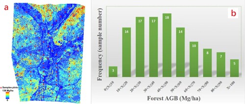
In this study, 113 AGB samples were taken from LiDAR-derived forest AGB maps for forest AGB inversion utilizing multi-frequency SAR datasets. They were first selected by a 750 m spatial interval fishnet sampling function using ArcGIS software through ArctoolBox and then several of them located on roads or bare ground were removed manually. The triangle points in Figure 2(a) show the spatial distribution of the final selected samples in this study. The detailed AGB information of the 113 samples and their group distribution with 10 Mg/ha interval are graphed in Figure 2(b).

2.3. Multi-frequency SAR data acquisition and preprocessing

We acquired full polarimetric airborne or spaceborne SAR data at X-, C-, L- and P bands for this study, a 30 m Shuttle Radar Topography Mission Digital Elevation Model (SRTM DEM) was also obtained for SAR data geocoding and terrain correction. X-, C-, and L band SAR data acquired in this study are spaceborne, they were from TerraSAR-X, RADARSAT-2, and ALOS-2 PALSAR-2, respectively. P band SAR data were from an airborne SAR system. The coverages of SAR data in each frequency obtained in this study are shown in Figure 1(a). Detailed parameters of multi-frequency SAR data are shown in Table 1.

Table 1. Detailed parameters of multi-frequency SAR data.

Sensor	Band	Incidence angle(°)	Range resolution(m)	Azimuth resolution(m)	Acquired date
TerraSAR-X	X	41.41	0.909	2.676	2015-08-19
RADARSAT-2	C	37.4–38.8	4.96	4.73	2013-08-20
ALOS PALSAR-2	L	36.52	2.86	2.64	2014-08-29
Airborne P band	P	50.06	0.63	0.67	2013-09-13

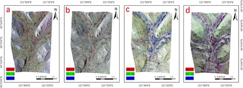
The common procedure of multi-frequency SAR data preprocessing includes: single-look complex (SLC) image conversion to Scattering matrix, radiometric calibration, multi-looking, filtering, terrain correction, and geocoding (Figure 3). Since the sensors to obtain SAR data at each frequency were different, the parameters for preprocessing them were slightly different. For example, the calibration constant, multi-looking factors, and filtering methods which differed from one frequency to another frequency are shown in Figure 3. Terrain corrections were compensated using a Geocoded Terrain Correction (GTC) model based on precise satellite orbit information. Multi-frequency SAR images were geocoded into the World Geodetic System-1984 (WGS-84) geographic coordinate system based on look-up tables between coordinates of SRTM DEM data and every SAR image. The SRTM DEM was sampled to 10 m resolution and mosaicked with 10 m DEM derived for LiDAR data at the test site. SAR images after preprocessing are displayed in Figure 4 using a Pauli RGB color map with a 10 m spatial resolution.

Figure 3. The overall workflow of multi-frequency SAR preprocessed.

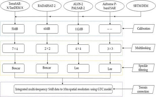
Figure 4. Pauli RGB (R:$|\mathrm{HH}-\mathrm{VV}|$, G: $|\mathrm{HV}+\mathrm{VH}|$, B: $|\mathrm{HH}+\mathrm{VV}|$) color map of X, C, L, P band SAR preprocessed. (a) X band. (b) C band. (c) L band. (d) P band.

3. Methodology

3.1. Multi-frequency SAR observation extraction

In this study, two model-based polarization decompositions named Freeman-Durden decomposition and Yamaguchi decomposition, and an eigen-based polarization decomposition named $H-A-\overline{\alpha }$ decomposition were used for original polarimetric observation extraction (Cloude and Pottier 1996). Several derivative observations of the three polarization decompositions were also introduced as polarimetric features in this study. Three backscatter coefficients from HH, HV, and VV channel and their ratios defined as radar vegetation index (RVI) and polarization distribution ratio (PDR) were used for forest AGB retrieval as well. In this study, 21 relevant observations (Table 2) were extracted from SAR full polarimetric data to explore the improvement potential of forest AGB inversion accuracy and the rough saturation point. We combined 21 features extracted from four frequency SAR data as 15 combinations such as X -, C -, L -, P -, X + C -, C + L -, X + L -, X + P -, C + P -, L + P -, X + C + L -, X + C + P, X + L + P, C + L + P, X + C + L + P.

Table 2. Names and meanings of 21 features of X-, C-, L- and P bands in this paper.

Features	Physical interpretation	Features	Physical interpretation
HH	Backscattering coefficient from HH channel	Y_ODD	Surface scattering component of Yamaguchi 4 decomposition
HV	Backscattering coefficient from HV channel	Y_VOL	Volume scattering component of Yamaguchi 4 decomposition
VV	Backscattering coefficient from VV channel	Y_HLX	Helix scattering component of Yamaguchi 4 decomposition
RVI	$\mathrm{RVI}={\displaystyle \frac{8\mathrm{HV}}{\mathrm{HH}+\mathrm{VV}+2\mathrm{HV}}}$	Entropy	Polarization scattering entropy
PDR	$\mathrm{PDR}={\displaystyle \frac{\mathrm{HH}-\mathrm{VV}}{\mathrm{HH}+\mathrm{VV}}}$	Anisotropy	Polarization scattering anisotropy
F_DBL	Double bounce scattering component of Freeman 3 decomposition	Alpha	Polarization average scattering angle
F_ODD	Surface scattering component of Freeman 3 decomposition	Beta	Scattering Entropy at 0° Azimuth angle
F_VOL	Volume scattering component of Freeman 3 decomposition	Delta	Scattering Entropy at 45° Azimuth angle
FD1	$\mathrm{FD}1={\displaystyle \frac{{\mathrm{F}}_{-}\mathrm{VOL}}{{\mathrm{F}}_{-}\mathrm{ODD}+{\mathrm{F}}_{-}\mathrm{DBL}}}$	Gamma	Scattering Entropy at 90° Azimuth angle
FD2	$\mathrm{FD}2={\displaystyle \frac{\mathrm{F\_VOL}}{\mathrm{F\_ODD}}}$	Lambda	Scattering Entropy at 135° Azimuth angle
Y_DBL	Double bounce scattering component of Yamaguchi 4 decomposition

3.2. Forest AGB inversion using different algorithms

In this study, considering the good performance of MLSR and RF in previous forest AGB estimations, both of them were selected as representative of parametric and nonparametric algorithms for AGB estimation here to investigate the potential of X, C, L, and P band polarimetric SAR observations and their combinations for forest AGB inversion. Meanwhile, the popular and widely used deep learning method of Keras based on Tensorflow is selected to explore the potentiality of deep learning methods in forest AGB estimation.

3.2.1. MLSR

MLSR inversion based on SAR features as input can be expressed as (2) (2) $y=a_0+a_1{x}_1+a_2{x}_2+\cdots +a_n{x}_n+\epsilon$(2) where $a_0$ is a constant, $x_1$, $x_2$, $\cdots$, $x_n$ are the extracted SAR observations, $a_1$, $a_2$, $\cdots$, $a_n$ are the regression coefficients associated with the corresponding SAR observations, $y$ is the value of the estimated forest AGB, $n$ is the number of explanatory SAR observations, and $\epsilon$ is the error term.

During the procedure of forest AGB estimation, the independent variables were introduced by MLSR one by one, then the significance of the influence from independent variables on the dependent variable $y$ was judged each time, the independent variables in the model were tested, and the insignificant variables from the model were removed one by one, at last, the optimal SAR observations and the inversion model were obtained. In this study, the SAR observations correlated high with AGB were selected under the condition that the significance value (p) is lower than 0.05. Readers are referred to Kabe (1963) for the detailed key steps of MLSR.

3.2.2. RF

The RF method combines several decision trees as an extension of the conventional single decision tree. RF reduces the higher variation in the prediction of a single decision tree resulting from over-fitted. The variation is reduced through the averaging of the outputs of each decision tree in the RF (Breiman 2001; Wang et al. 2019). The principle of estimating forest AGB by RF is as follows: Each decision tree's root node samples are chosen randomly from K-measured AGB sample sets in the training samples, and the same number of decision trees is produced at the same time. Then certain features are randomly selected for each built decision tree. Here, row sampling is conducted through a bootstrap algorithm and then column sampling is conducted for the input SAR features with the most appropriate feature selected as the split node. After the RF is established, K estimation results are obtained and the average value of the K estimation results is taken as the final estimated AGB result of each pixel.

3.2.3. Keras using TensoFlow as a backend

A deep learning algorithm generally includes two levels of framework: the low-level framework and the high-level framework. The low-level framework usually was written in quite long codes for preparing the final deep learning model. Tensorflow is the most popular low-framework and easy to develop other parts on it. Keras is a widely used high-level framework written in Python and here it is used in R software through the Keras library. In this study, Keras is used as a high-level framework based on the low-level framework of TensorFlow. The flowchart of the deep learning algorithm used is shown in Figure 5.

Figure 5. Flowchart of the deep learning algorithm.

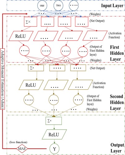
A total of three dense layers were constructed in this study. The first layer has 8 neurons, the next one has 4 neurons, and the final one has 1 neuron. According to our input SAR features, the input shape parameters are set as 21, 42, 63, and 84, respectively. The weight values for every neuron are randomly assigned and modified later according to the optimizer function. A Rectified Linear Unit (ReLU) is used as the activation function to ensure the contribution of neural input from the previous layer to the final output. The mean absolute error (MAE) is set as a loss function. It is calculated using the LiDAR-derived AGB value and the predicted value after the prediction of the final layer. The next adaptive moment estimation (Adam) works as an optimizer function to recalibrate the weight of the neurons by observing the changes in the loss function. A total of 113 LiDAR-derived AGB values work as field-collected true values. These points were randomly divided into 10 parts for model training and 10-fold cross-validation of the estimated results. 750 or 800 epochs with a batch of 29 were set for the deep learning model. To avoid model overfitting, a patience value of 40 is applied for an early stop.

3.3. Forest AGB validation method

To validate the obtained results of forest AGB retrieved by MLSR and RF algorithms, three statistical indicators including determination coefficient (R², Equation (4)), root mean square error (RMSE, Equation (5)), and relative accuracy (rRMSE, Equation (6)) are used here for validation. The estimated AGB values and the LiDAR-measured AGB values are correlated using a factor called R², and the closer R² is to 1, the more accurate the results. The RMSE value indicates how far the observed value deviates from the true value; the lower the RMSE value, the more accurate the predicted AGB value, and the better the performance of the inversion models. The estimation accuracy is higher when the rRMSE values are lower. (4) $R^2=1-{\displaystyle \frac{\sum _{i=1}^m{(y_i-{\hat{y}}_i)}^2}{\sum _{i=1}^m{(y_i-{\overline{y}}_i)}^2}}$(4) (5) $\mathrm{RMSE}=\sqrt{{\displaystyle \frac{1}{m}\sum _{i=1}^m{(y_i-{\hat{y}}_i)}^2}}$(5) (6) $\mathrm{rRMSE}={\displaystyle \frac{\mathrm{RMSE}}{{\overline{y}}_i}\times 100\text{\%}}$(6) where $m$ is the sample size, ${\hat{y}}_i$ is the estimated value of forest AGB, $y_i$ is the measured value of forest AGB, and ${\overline{y}}_i$ is the average value of forest AGB.

4. Results and analysis

The abundance of multi-frequency data sources makes it possible to combine the advantages of each frequency to improve the performance of SAR data in forest AGB inversion. In this study, 21 polarimetric SAR features were first extracted from X, C, L, and P band full polarimetric SAR data, respectively. Then, a total of 84 features of the four bands were combined in 15 different ways and worked as independent variables for the inversion models of forest AGB estimation. The performance of each combination in forest AGB estimation was fully explored based on representatives of a parametric model like MLSR, a nonparametric model like RF, and a deep learning algorithm of Keras using TensofFlow as a backend. R², RMSE and rRMSE calculated according to the estimated AGB and LiDAR-derived AGB were presented here for the evaluation of their inversion capability.

4.1. Forest AGB retrievals using MLSR algorithms

MLSR algorithms were applied for forest AGB estimation using a total of 15 combinations of four-band SAR observations in the test site. MLSR performed well with most of the rRMSE values around or lower than 35%. Their performances were divided into 4 groups according to the input number of SAR observations. Four members like each single band grouped as the first group, here four MLSR algorithms were built according to 21 input SAR features at each frequency, respectively. Six members like combinations of each dual-band involved in 42 SAR observations were grouped as the second group, the combinations of X and C band (X + C), X and L band (X + L), X and P band (X + P), C and L band (C + L), C and P band (C + P), and L and P band (L + P), six MLSR algorithms were built according to 42 input SAR features at each combination, respectively. Four members of each tri-band involved in 63 SAR observations were grouped as the third group, they included the combinations of X, C, and Lband (X + C + L), X, L, and P band(X + L + P), X, C, and P band (X + C + P), and C, L, and P band (C + L + P), four MLSR algorithms were built according to 63 input SAR features at each combination, respectively. The fourth group only included a member, it is the combination of X, C, L and P bands, an MLSR algorithm was built according to all the 84 SAR features working as model input. Table 3 summarizes the performance of 15 different multi-frequency SAR observation combinations.

Table 3. Forest AGB retrieval results based on MLSR multi-frequency SAR combination.

Band combination	MLSR fit model	R^2	RMSE (Mg/ha)	rRMSE (%)
X	AGB = 269.02 + 8.32XFD2-5.92Xalpha	0.26	21.81	46.67
C	AGB = −5.57 + 563.26CVV	0.19	22.79	48.77
L	AGB = −179.04 + 422.22LVV + 2.18LFD2-202.71LFVOL + 214.49Lentropy	0.59	16.18	34.62
P	AGB = 178.77 + 45.98PYVOL-2.81Pbeta	0.53	17.34	37.11
X + C	AGB = 233.19 + 316.38CVV-4.86Xalpha	0.28	21.54	46.09
X + L	AGB = −44.04 + 428.27LVV + 1.26LFD2 + 205.38LFDBL-342.66Llambda + 0.76Xgamma	0.58	16.36	35.02
X + P	AGB = 225.58 + 42.59PYVOL-2.36Pbeta + 7.02XVV	0.58	16.39	35.08
C + L	AGB = 31.10 + 1.73LFD2 + 2.44LFDBL-1.11LPDR-1.88CYHLX	0.57	16.65	35.63
C + P	AGB = 89.17-166.56PVV + 2.68PFD1 + 48.71PYVOL-1.45Pbeta + 311.24CVV	0.62	15.70	33.59
L + P	AGB = 99.69-126.54PVV + 4.54PFD1-2.13Pbeta-48.47PRVI + 103.95LVV + 2.30Lalpha	0.67	14.51	31.04
X + C + L	AGB = −21.12 + 1.62LFD2 + 2.46LFDBL-9.76LPDR-1.88CYHLX + 7.69Xgamma	0.58	16.46	35.23
X + C + P	AGB = 91.07-163.93PVV + 2.61PFD1 + 51.04PYVOL-39.80PYHLX −1.47Pbeta + 312.89CVV	0.61	15.85	33.91
X + L + P	AGB = 89.17-166.56PVV + 2.68PFD1 + 48.71PYVOL-1.45Pbeta + 311.24CVV	0.62	15.70	33.59
C + L + P	AGB = 265.00-121.61PVV + 4.68PFD1-2.25Pbeta-54.37PRVI + 98.95LVV + 2.29Lalpha-176.75Centropy	0.67	14.47	30.97
X + C + L + P	AGB = 314.05-104.28PVV + 4.62PFD1-2.71Pbeta-63.20PRVI + 581.53LYHLX + 1.38Lalpha-201.32Centropy + 0.72Xgamma	0.68	14.36	30.73

Table 3 reveales the better performance of MLSR for forest AGB estimation. The MLSR performed better both with longer wavelength SAR observations and their combination with other frequency observations. For example, using the combinations of tri-frequency and quad-frequency SAR observations with MLSR algorithms, the R² values acquired between the estimated AGB and LiDAR-derived AGB ranges from 0.58 to 0.68 and the rRMSE values range from 14.36 Mg/ha to 16.46 Mg/ha.

As shown in Table 3, the best performances using single-frequency observation are L band with R² = 0.59, RMSE = 16.18 Mg/ha, and rRMSE = 34.62%. The backscatter coefficients from VV (LVV), the FD2, F_VOL and entropy played an important role in the forest AGB retrieval procedure when using L band polarimetric SAR observations. Next was P band with R² = 0.53, RMSE = 17.34 Mg/ha, and rRMSE = 37.11%. Among the acquired 21 SAR parameters, only Y_VOL and beta were selected as the most important SAR features for AGB estimation. The performance of combinations of dual-frequency in forest AGB inversion improved obviously except L-band, especially for the combination with short bands like X and C bands. The results of combinations of dual-frequency showed an obviously higher determination coefficient and also a lower relative RMSE (rRMSE) for ground measurements. Among them, the retrieval performance of the combination of the L and P bands was the best (R² = 0.67, RMSE = 14.51 Mg/ha, and rRMSE = 31.04%), followed by the combination of C and P (R² = 0.62, RMSE = 15.70 Mg/ha, and rRMSE = 33.59%). Combing with a long band like the L or P band, better retrieval performance was obtained compared to using a single C or X band, and the improvements of rRMSE were higher than 10%. More of the selected important SAR features were from the longer wavelength among the combinations of dual-frequency. The backscatter coefficient from the VV channel showed the highest frequency in the most important feature to characterize the change of AGB, the next was the polarimetric feature of Vol.

Compared with the best performance of two dual-frequency combinations like the C + P band and the L + P band, the combinations of tri-frequency showed no obvious improvement for forest AGB inversion. The combination of the C + L + P band had the highest accuracy in retrieving forest AGB with R² of 0.67, RMSE of 14.47 Mg/ha, and rRMSE of 30.97%. The results revealed that combinations of tri-frequency SAR data can improve the retrieval accuracy of forest AGB compared with single frequency but no great improvement compared with combinations of dual-frequency, especially for the combinations combined with the L or P band. Most of the polarimetric SAR features from the P band were selected as the important SAR features for forest AGB estimation using tri-frequency combinations, among them, Beta from the P band showed the highest frequency. The combination of four-frequency performed best in forest AGB among all of the 15 combinations of X, C, L, and P band SAR polarimetric observations (R² = 0.68, RMSE = 14.36 Mg/ha, and rRMSE = 30.73%). However, the results were similar to the performance of the combination of L + P (R² = 0.67, RMSE = 14.51 Mg/ha, and rRMSE = 31.04%.) and the combination of C + L + P (R² = 0.67, RMSE = 14.47 Mg/ha, and rRMSE = 30.97%). They were only slightly higher than the retrieved results using a single L band (R² = 0.59, RMSE = 16.18 Mg/ha, and rRMSE = 34.62%.) and a P band (R² = 0.53, RMSE = 17.34 Mg/ha, and rRMSE = 37.11%).

In Table 3 we found that VV, FD2, and VOL were frequently selected as optimized SAR observations for obtaining forest AGB with better performance, especially using L and P band features. The results revealed that at the C band, extinction of VV is obvious and most of them happened in the needles of trees at the canopy although VV is sensitive to the change of AGB, it is easy to get saturated and then only obtained low estimation accuracy at the C band. The extinction of VV at the L band may result from big branches or stems of the trees in the forest and then can better reflect the change of forest AGBs. FD2 is the ratio of volume scattering and surface scattering and is sensitive to the extinction of the forest since the better penetration capability of the L band in the forest, the feature is also selected as the optimal for forest AGB estimation. The VOL extracted from Freeman-Durden decomposition was selected as the optimal feature for forest AGB estimation using L band SAR observations while VOL extracted from Yamaguchi decomposition was selected as the optimal for forest AGB estimation using P band SAR observations, the phenomenon revealed that the developed volume component in Yamaguchi decomposition is more suitable for interpreting forest scattering mechanism at the P band while the component from Freeman-Durden decomposition interprets the forest scattering mechanism at the L band better. For the inversion using combinations from dual-frequency, tri-frequency, and quad-frequency SAR observations, the most optimal features selected came from the longer bands and confirmed the better performance of L-band SAR observation for forest AGB estimation. The above features which performed better in a single frequency also performed as optimal features in the combined SAR observations, except that DBL extracted from the L band seems sensitive to the change of forest AGB when SAR observation combinations were used for forest AGB estimation.

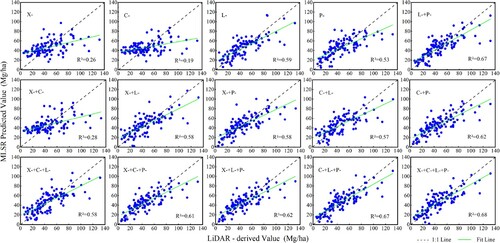
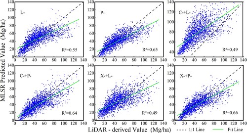
Figure 6 shows the 15 scatterplots created by the estimated AGB values using 15 group SAR observations by MLSR algorithms and the measured values by the LiDAR product. The scatterplots presented here were used for observing the potential saturation point for forest AGB estimations using different groups of SAR observations. The saturation points were determined according to the turning points when the predicted values remained the same while the LiDAR-derived AGB values kept increasing. As shown in Figure 6, the overestimation of low forest AGB values and the underestimation of high forest AGB values at the X and C bands were more obvious than those at the L and P bands. By observing the patterns of each sub-scatterplot, we found the saturation points of the L and P bands were relatively high, reaching 90 Mg/ha and they were lower at the X and C bands, where the values were around 60 Mg/ha. The scatter plots of forest AGB retrieved by dual-frequency SAR combinations showed an obvious increase in inversion accuracy and saturation points. The saturation points of the combinations of X + L - and L + P - bands were relatively high, reaching 100 Mg/ha. The saturation points of the X + C band were relatively low,about 60 Mg/ha. Five dual-frequency combinations including X + L, X + P, C + L, C + P, and L + P showed good fitting and the values of the scatter points were roughly distributed on both sides of the line with strong correlations with observed AGBs. For the tri-frequency SAR combinations, despite the ligh improvement of forest AGB inversion accuracy of using tri-frequency combinations, the saturation point of each combination became stable at around 90∼100 Mg/ha. The saturation points for the combination of X + C + L + P band SAR observations was around 110 Mg/ha. The saturation points observed according to Figure 5 revealed the effective performance of using the dual-frequency SAR observations, especially the combination of the L or P band with higher frequency SAR observations. They confirmed the better performance of the L and P bands for forest AGB estimation.

Figure 6. Results of forest AGB retrieved by MLSR based on 15 combinations of different frequency SAR observations.

4.2. Forest AGB retrievals using RF algorithms

After analyzing the performance of MLSR models to estimate forest AGB using 4 groups and 15 different SAR observation combinations, this section showed the forest AGB retrieved by RF algorithms. The algorithms were trained by all of the samples and validated by the 10-fold validation. For the RF algorithms, the number of regression trees (ntree) and the number of input SAR observations per node (mtry) are two key model parameters for forest AGB inversion. In this study, the optimal number of decision trees for each combination was decided by the minimum RMSE value between the estimated and LiDAR-derived AGB measurement and they were set as 100 in each inversion procedure. The number of input SAR observations per node was tested for 1/3 of the whole number of input SAR observations. Table 4 summarizes the retrieved results by RF models using 15 different multi-frequency SAR observation combinations for forest AGB inversion.

Table 4. Forest AGB retrieval results based on RF with multi-frequency SAR combination.

Band combination	R^2	RMSE (Mg/ha)	rRMSE (%)	Band combination	R^2	RMSE (Mg/ha)	rRMSE (%)
X	0.30	21.20	45.37	C + P	0.63	15.33	32.80
C	0.38	20.02	42.85	L + P	0.64	15.20	32.53
L	0.55	16.92	36.21	X + C + L	0.58	16.50	35.30
P	0.61	15.85	33.92	X + C + P	0.64	15.18	32.49
X + C	0.39	19.88	42.54	X + L + P	0.65	15.11	32.33
X + L	0.55	17.07	36.53	C + L + P	0.65	14.92	31.93
X + P	0.63	15.36	32.86	X + C + L + P	0.66	14.81	31.69
C + L	0.59	16.29	34.86

Table 4 determines that RF algorithms improved the inversion performance of single frequencies like X, C, and P band observation. For the combinations of dual-frequency, tri-frequency, and quad-frequency, RF algorithms showed similar performance as MLSR algorithms. Although it has better performance in single frequencies, the results confirmed the better performance of the L or P band than the X or C band as well. For the single-frequency SAR observations, the P band performed best in the four frequencies for forest AGB inversion with R² = 0.61, RMSE = 15.85 Mg/ha, and rRMSE = 33.92%. L band followed the P band with R² = 0.55, RMSE = 16.92 Mg/ha, and rRMSE = 36.21%. Among the dual-frequency combinations, the best results were obtained by the combination of the L + P band with R² = 0.64, RMSE = 15.20 Mg/ha, and rRMSE = 32.49%. While for the other combinations of dual-frequency SAR observations, especially for the combinations of a low frequency and a high frequency like X + L, X + P, C + L, and C + P, the rRMSE value decreased no more than 5% compared with the performance of the combination of the L + P band. Similar to the performance of MLSR models using tri-frequency SAR observation combinations, the results showed no obvious improvement in forest AGB estimation especially compared with better performance of dual-frequency combinations like X + P, C + P, and L + P bands. The tri-frequency combinations including the P band showed high inversion accuracy with R² = 0.64 or 0.65 and rRMSE values were around 32%. The combination of four frequencies obtained the highest accuracy with R² = 0.66, RMSE = 14.81 Mg/ha, and rRMSE = 31.69%. The performance of RF algorithms agreed with the effective performance of using dual-frequency SAR observations for forest AGB estimation and the better performance of L and P band single-frequency SAR observation.

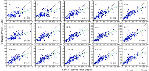
Figure 7 presents the 15 scatterplots created by the estimated AGB values using 15 group SAR observations by RF algorithms and the measured values by LiDAR products. According to the scatterplots, the saturation points showed no obvious change compared to the performance of using MLSR with each combination of different frequency SAR observations. For the performance of single-frequency SAR observations, the retrieved forest AGB values matched better with LiDAR-derived measurements with a saturation point around 90 Mg/ha for the L and P bands, and 70 Mg/ha for the X and C bands. For the performance of dual-frequency SAR observations, the turning points between overestimation and underestimation were about 50 Mg/ha. Before 50 Mg/ha, for the combinations of X + C, X + L, C + L bands, the overestimation of low AGB values was obvious, and after 50 Mg/ha, it showed a clear underestimation for high AGB values. For the combinations of X + P, C + P, L + P bands, the overestimation for low AGB values was not significant when AGB values were less than 50 Mg/ha but it showed obvious underestimation for AGB values greater than 50 Mg/ha. The results revealed the better performance of P band SAR observations for forest AGB estimation. They also demonstrated that other bands may improve their AGB retrieval capability when they were combined with P band observations. The saturation points for tri-frequency and quad-frequency SAR observations were around 100 Mg/ha. The pattern of the scatter plots revealed that the saturation phenomenon still existed using the polarimetric SAR observation combinations, but it showed obvious improvement compared with using single-frequency SAR observations for forest AGB estimations.

Figure 7. Results of forest AGB retrieved by RF based on 15 combinations of different frequency SAR observations.

4.3. Forest AGB retrievals using deep learning algorithms

Table 5 summarizes the forest AGB estimation results using the deep learning method and 15 combinations of different frequency SAR polarimetric observations. Single-frequency SAR measurements performed worse than combinations of dual-frequency, triple-frequency, and quad-frequency SAR observations. The combined X and P bands obtained the highest estimation accuracy with R² = 0.59, RMSE = 16.45, and rRMSE = 35.21%. Next was the combination of X and L with R² = 0.50, RMSE = 18.21, and rRMSE = 38.97%. While for the performance of MLSR and RF, most of the RMSE values were lower than 38%. The worse performance of the deep learning method may result from the abnormal estimates shown in Figure 8. The estimated values of several samples are zero and then result in the higher RMSE values and rRMSE values.

Figure 8. Results of forest AGB retrieved by the deep learning algorithms based on 15 combinations of different frequency SAR observations.

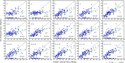
Table 5. Forest AGB retrieval results based on deep learning with multi-frequency SAR combination.

Band combination	R^2	RMSE (Mg/ha)	rRMSE (%)	Band combination	R^2	RMSE (Mg/ha)	rRMSE (%)
X	0.07	32.34	69.31	C-+P-	0.23	27.18	58.16
C	0.03	28.02	59.94	L-+P-	0.59	16.45	35.21
L	0.27	24.12	51.58	X-+C-+L-	0.25	26.88	57.52
P	0.20	27.79	59.46	X-+C-+P-	0.26	26.93	57.63
X + C	0.22	22.74	48.65	X-+L-+P-	0.36	23.04	49.31
X + L	0.50	18.21	38.97	C-+L-+P-	0.40	22.05	47.19
X + P	0.34	23.16	49.55	X-+C-+L-+P-	0.37	24.64	52.74
C + L	0.35	22.49	48.13

4.4. Comparison and analysis of forest AGB mapping with the best inversion model

In this paper, the extracted 84 SAR features were used to carry out forest AGB inversion in the study area through MLSR and RF inversion models in 4 combination groups of single-frequency, dual-frequency, tri-frequency, and quad-frequency. By comparing and analyzing the retrieved results using MLSR and RF algorithms, we found the best results were obtained by the MLSR model with the combination of quad-frequency SAR observations. The MLSR algorithm was used for the AGB mapping of the whole test site (Figure 9(a)), and the map was sampled in a spatial resolution of 10 m and compared with LiDAR-derived AGB map (Figure 9(b)).

Figure 9. Forest AGB mapped by MLSR algorithms and forest AGB product from LiDAR. (a) Forest AGB mapped by MLSR; (b) Forest AGB product from LiDAR.

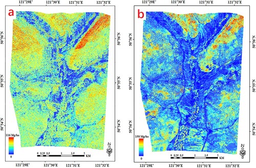
Since the 10 parts of the samples were randomly selected for model training and 10-fold cross-validation, the trained models were slightly different each time. We averaged three times estimation results to map the terminal results (Figure 9(a)). The lowest value is normalized into 0 Mg/ha according to reality. The highest forest AGB value in the MLSR obtained map in the test site was 116 Mg/ha, while the maximum value of LiDAR-derived AGB map used for model training and validation was 150 Mg/ha. The difference may result from the overestimation of low AGB values and THE underestimation of high AGB values in the test site. In the area covered by road without any forest, the average AGB value was 6 Mg/ha which confirmed the overestimation of the built MLSR algorithm. In the area in the upmiddle and upright of the study area, where the AGB was higher than 60 Mg/ha, the MLSR obtained map showed obvious underestimation compared with the LiDAR-derived AGB map.

In reality, the demand for data volume of L and P combination is smaller while the combinations of low and long frequencies are more available, practical and easy to implement. Considering these here six other combinations of multiple frequencies including L, P, C + L, C + P, X + L, and X + P were utilized for mapping the AGB in the study area. The maps were generated with the randomly trained models, the non-forest-covered area was masked and the mapped product is shown in Figure 10. According to the definition of AGB, the point-to-point correlations between estimated maps and LiDAR-derived maps were graphed as Figure 11 based on a neighbor analysis with a window of 100 m. Table 5 summarizes the accuracy of the map products with six combinations of SAR observations.

Figure 10. Forest AGB map examples derived by MLSR algorithms.

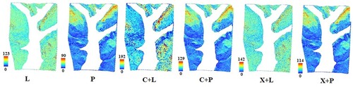
Figure 11. Results of forest AGB retrieved by MLSR algorithms.

According to Figure 10, the AGB maps generated using MLSR with different frequency SAR observables were remarkably different as they rely on different SAR features (Table 3). Different features showed different responses to different AGB levels and then they showed obviously different trends or patterns in the AGB maps in Figure 10. P band in the single-frequency, and dual-frequency combinations including C + P and X + P showed similar performance with rRMSE values around 30%. L band and the combinations of it with C and X showed a lighter decrease compared with the results shown by randomly sampled plots on LiDAR-derived AGB products. Most areas of the maps derived by using the L band, X + L, and C + L showed obvious underestimation of high AGB values and overestimation of low AGB values. For the map derived by C + L SAR observations showed misestimated higher AGB values of 150 Mg/ha.

The summarized accuracy results of the map products confirmed the good performance of the P band and the combinations with the other two low-frequency SAR observations. Although the performance of the L band showed a slight decrease, the rRMSE values are around 32% except for the performance of combined C and L band SAR observations, the higher rRMSE (76.25%) may result from the outlier occurred at higher estimated AGB values in the east of the test area (Table 6). However, the reason needs to be further explored in the future.

Table 6. Forest AGB retrieval results according to the mapped results in the test area.

Band combination	R^2	RMSE (Mg/ha)	rRMSE (%)	Band	R^2	RMSE (Mg/ha)	rRMSE (%)
L	0.55	15.38	32.75	X + L	0.49	16.66	35.49
P	0.65	14.77	31.45	X + P	0.66	14.50	30.87
C + L	0.49	35.81	76.25	C + P	0.64	15.45	32.91

5. Discussion

Previous studies have explored the capability of backscatter observations extracted from single frequency and their combinations for forest AGB inversion. The results demonstrated the potential of forest inversion accuracy improvement with the combination of multi-frequency backscatter observations (Breiman 2001; Cartus et al. 2019; Cloude and Pottier 1996; Englhart, Keuck, and Siegert 2011; Feng et al. 2016; Gao et al. 2018; Harrell et al. 1995; Imhoff 1995; Kurvonen, Pulliainen, and Hallikainen 1999; Pang et al. 2016; Ranson and Sun 1994; Saatchi et al. 2007; Santi et al. 2017; Santoro et al. 2019; Wang et al. 2019). However, since some of them added multi-temporal information, whether the improvement resulted from the integration of multi-temporal observations or the integration of the multi-frequency observations remained unclear. In this study, four popular microwave frequencies at X, C, L, and P bands in forest AGB retrieval were selected to fully explore the potential of the combination of multi-frequency SAR data on forest AGB estimation. MLSR, RF, and deep learning algorithms were utilized for forest AGB inversion, respectively. As the growing archives of quad-polarimetric SAR images at each band, polarimetric and backscatter observations were both extracted in this study to estimate forest AGBs.

To understand in more detail whether the combination of multi-frequency SAR observations can improve the forest AGB inversion accuracy and how combining them will perform best in forest AGB estimation, 15 combinations with 4 single-frequency, 6 dual-frequency combinations, 4 tri-frequency combinations, and 1 quad-frequency combination were applied with MLSR, RF and deep learning algorithms to retrieval forest AGB in the test sites. According to the results, we determined that the combination of quad-frequency obtained the best performance both by MLSR (rRMSE = 30.73%, corresponding to an RMSE of 14.36 Mg/ha) and RF (rRMSE = 31.69%, corresponding to an RMSE of 14.81 Mg/ha) algorithms. However, the improvement of estimation accuracy was not significant compared with the inversion results obtained with dual-frequency combinations of L + P (rRMSE = 31.04% and RMSE = 14.51 Mg/ha with MLSR; rRMSE = 32.49% and RMSE = 15.20 Mg/ha with RF), C + P (rRMSE = 33.59% and RMSE = 15.70 Mg/ha with MLSR; rRMSE = 32.80% and RMSE = 15.33 Mg/ha with RF) and the results obtained by the L band with MLSR (rRMSE = 34.62% and RMSE = 16.18 Mg/ha) and the P band with RF (rRMSE  = 33.92%, RMSE = 15.85 Mg/ha). Moreover, the performance of high-frequency band (X or C) is significantly improved when combined with one or two low-frequency bands (L or P bands). In contrast, the improvement is not obvious for a high-frequency band when it is combined with a high frequency. Meanwhile, both the MLSR and RF performed well in forest AGB estimation using different combinations of SAR observations. The results acquired with the deep learning algorithms showed quite different with the performance of MLSR and RF. The best and better performances were obtained by the combination of L + P and X + L with RMSE = 16.45 Mg/ha and RMSE = 18.21 Mg/ha, respectively. Deep learning algorithms performed worse with single-frequency SAR observables with all of the R² less than 0.3, it may result from that it is difficult for deep learning methods to detect the useful characterization from single SAR measurements. While more sensitive features added in the combination of dual-frequency and the ratio of the training samples and input features in the algorithms are more suitable, several combinations of dual-frequency showed better performance than triple-frequency combinations and quad-frequency combinations.

Adding polarimetric observations for forest AGB inversion using multi-frequency SAR measurements allowed for obvious saturation point improvement and estimation errors decreased. A previous study reported that the saturation point of the backscatter coefficient on the C band is about 20 Mg/ha, for the L band is about 40 Mg/ha, and for the P band is about 70 Mg/ha, the results were obtained from a Hawaiian tropical rain forest (Imhoff 1995). Other studies confirmed the saturation limit and determined it is affected by forest structure (Lu et al. 2016; Lucas et al. 2007; Luckman et al. 1997). In this study, the saturation points of the X and C bands are around 60–70 Mg/ha and it is around 90–100 Mg/ha for the L or P band, the results showed obvious improvement of the saturation points for different bands. Cartus et al. (2019) report an error of 32% for a boreal forest using P band backscatter coefficients and a parameter inversion algorithm, 51% for the C band and 50% for the L band. The findings showed that the P band is the frequency best suited for predicting forest AGB and that combining the P band with observations obtained at higher frequency only yields modest improvements. The outcomes are consistent with the findings of this investigation. When comparing the performance of the combined C and P bands with the performance of the single P band in our investigation, the estimation accuracy only increased by 5%. Multi-frequency backscatter observations applied for a tropical forest AGB estimation found P band allowed for the highest accuracy for AGB estimation among all the combinations of X, C, L, and P band observations. Several dual-frequency combinations such as P and C bands, P and X bands, L and X bands, or L and C bands even resulted in poor performance than the results acquired by a single P band. It also demonstrated that the combinations of tri-frequency SAR observations resulted in poor accuracies compared with the combinations of dual-frequency and even single-frequency (Cartus and Santoro 2019). The above analysis revealed that the P band is the most suited frequency for forest AGB inversion, the combination of a lower- frequency SAR observations and a higher-frequency SAR observations allows a forest AGB estimates with relatival errors of 30%∼40%. Combinations of more than three frequency SAR observations only resulted in limited improvement of forest AGB retrieval accuracy. The results agreed with the mapping results performed using single-frequency and dual-frequency SAR observations in this study.

Lu et al. (2016) grouped forest AGB inversion models into two broad categories: parametric and nonparametric algorithms. In this study, a parametric algorithm named MLSR and a nonparametric named RF were applied for forest AGB estimation using combinations of multi-frequency SAR observations and each single SAR observation. Deep learning algorithms were developed as a subfield of nonparametric algorithms and can recognize intricate nonlinear patterns in data by mimicking the neural architecture of human brains (Beysolow 2017). MLSR and RF algorithms were suitable for forest AGB estimations, there are no obvious differences in the performance of MLSR and RF. Previous studies only used parametric algorithms for forest AGB estimation using combinations of multi-frequency SAR observations, one is the regression model (Englhart, Keuck, and Siegert 2011), the other is the Water-cloud-type model (Cartus et al. 2019; Cartus and Santoro 2019; Santoro et al. 2019). Englhart, Keuck, and Siegert (2011) explored the potential of the combination of X and L band SAR data for a tropical forest AGB retrieval. The results confirmed the robustness and transferability of the regression model for forest AGB estimation using combined X and L band SAR observations, the R² for the built regression models was higher than 0.7, and the highest R² between the estimated AGB values and field measurements was 0.53. The potential of the Water-cloud type model applied in multi-frequency SAR observations was explored in boreal and tropical forests. With this approach, AGB estimates in tropical forests were obtained with rRMSE ranging from 30% to 45% when using single X, C, L, and P bands. For the combinations of dual-frequency and tri-frequency SAR observations, rRMSE values ranged from 32% to 43% (Cartus and Santoro 2019). AGB estimates in boreal forests were obtained with rRMSE ranging from 40% to 55% when using single X, C, and L bands. For the combinations of dual-frequency and tri-frequency SAR observations, all of the rRMSE values were less than 50% (Cartus et al. 2019). In our study, the rRMSE values range from 34% to 47% for single-frequency using MLSR algorithms and 33% to 46% for RF algorithms. For combinations of dual-frequency, tri-frequency, and quad-frequency SAR observations, the ranges are 30%∼47% when using MLSR algorithms and 31%∼43% when using RF algorithms. The earliest application of deep learning algorithms in forest AGB estimation was in 2014 in an Indian mangrove (Manna et al. 2014), while combined with multi-frequency SAR observables were not explored yet. Ghosh and Behera (2021) demonstrated the better performance of forest AGB estimation in an Indian mangrove forest with high spatial heterogeneity. In this study, the better performance of MLSR and RF may result from the quite homogeneous forest type in the test site. In the homogeneous forest, changes in the stand AGBs and their associated polarimetric scattering mechanisms would be in proportion, as observed by SAR sensors. In the heterogeneity forest, with suitable training samples and input features, a deep learning method had better study capability and easy to obtain good estimation results.

6. Conclusions

In this paper, 15 combinations of X, C, L, and P band SAR observations are used to fully explore the capability of combinations of multi-frequency SAR observations for forest AGB estimation. In this study, MLSR, RF, and a deep learning algorithm are used as representatives of inversion models for forest AGB estimation using multifrequency SAR measurements. At each frequency, 21 SAR observations, including backscatter coefficients from HH, HV, and VV channels and polarimetric features from three polarimetric decomposition methods were extracted and used for forest AGB retrieval. It concluded that (1) Adding polarimetric information allows for the improvement of saturation points in forest AGB retrieval. In single-frequency SAR observations, the saturation point of the X band and C band SAR observations is 60–70 Mg/ha, and the saturation point of combined L and P band SAR observations is 90–100 Mg/ha. (2) The L and P bands are more suitable frequencies for estimating forest AGB, only limited improvements can be achieved by combining them with the X and C bands. Combined P band with any other frequency allowed for retrieving a forest AGB with comparable accuracy as tri-frequency observations and quad-frequency observations. The combinations of X and C bands showed limited improvement in inversion accuracy compared with single X or C observations. (3) The performance of MLSR and RF models in retrieving forest AGB using 15 multi-frequency SAR observations seems no obvious difference. Deep learning algorithms showed better performance than MLSR and RF. (4) The inversion using dual-frequency SAR polarimetric observations (including a high frequency and a low frequency) and P band SAR polarimetric observation have similar performance and are more practical in reality for forest AGB mapping and retrieval. However, since the unavailable of all X, C, L and P band quad polarimetric SAR images at other test sites, in this study, only a test site was selected for the exploration of the potential of multi-frequency combinations for forest AGB retrieval, in the future, with P band images supported by BIOMASS mission, further similar studies need to be explored in other test sites.

Acknowledgements

We sincerely thank the Research Laboratory of Remote Sensing Application Technology, Institute of Resource Information, Chinese Academy of Forestry Sciences, for providing the data used in this study.

Disclosure statement

No potential conflict of interest was reported by the author(s).

Additional information

Funding

This work was supported by the National Natural Science Foundation of China [grant numbers 32160365, 42161059, 32371869, and 31860240] and the Yunnan Province agriculture joint special project [grant number 202301BD070001-058].

References

- Beysolow, T. 2017. “Introduction to Deep Learning Using R.” In Introduction to Deep Learning Using R – a Step-by-Step Guide to Learning and Implementing Deep Learning Models Using R, 1–9. Berkeley, CA: Apress. https://doi.org/10.1007/978-1-4842-2734-3_1.
- Bortolot, Z. J., and R. H. Wynne. 2005. “Estimating Forest Biomass Using Small Footprint LiDAR Data: An Individual Tree-Based Approach That Incorporates Training Data.” ISPRS Journal of Photogrammetry & Remote Sensing 59 (6): 342–360. https://doi.org/10.1016/j.isprsjprs.2005.07.001.
- Breiman, L. 2001. “Random Forests.” Machine Learning 45 (1): 5–32. https://doi.org/10.1023/A:1010933404324.
- Cartus, O., and M. Santoro. 2019. “Exploring Combinations of Multi-Temporal and Multi-Frequency Radar Backscatter Observations to Estimate Above-Ground Biomass of Tropical Forest.” Remote Sensing of Environment 232:111313. https://doi.org/10.1016/j.rse.2019.111313.
- Cartus, O., M. Santoro, U. Wegmüller, and B. O. R. Rommen. 2019. “Benchmarking the Retrieval of Biomass in Boreal Forests Using P-Band SAR Backscatter with Multi-Temporal C-and L-Band Observations.” Remote Sensing 11 (14): 1695. https://doi.org/10.3390/rs11141695.
- Chowdhury, T. A., C. Thiel, C. Schmullius, and M. Stelmaszczuk-Górska. 2013. “Polarimetric Parameters for Growing Stock Volume Estimation Using ALOS PALSAR L-Band Data Over Siberian Forests.” Remote Sensing 5 (11): 5725–5756. https://doi.org/10.3390/rs5115725.
- Cloude, S. R., and E. Pottier. 1996. “A Review of Target Decomposition Theorems in Radar Polarimetry.” IEEE Transactions on Geoscience and Remote Sensing 34 (2): 498–518. https://doi.org/10.1109/36.485127.
- Englhart, S., V. Keuck, and F. Siegert. 2011. “Aboveground Biomass Retrieval in Tropical Forests – the Potential of Combined X-and L-Band SAR Data Use.” Remote Sensing of Environment 115 (5): 1260–1271. https://doi.org/10.1016/j.rse.2011.01.008.
- Feng, Q., E. X. Chen, Z. Y. Li, L. Li, and L. Zhao. 2016. “Estimation Method of Forest Aboveground Biomass in Complex Terrain Based on Airborne P-Band Fully Polarized SAR Data.” Forestry Science 52 (3): 10–22. https://doi.org/10.11707/j.1001-7488.20160302.
- Ferrazzoli, P., and L. Guerriero. 1995. “Radar Sensitivity to Tree Geometry and Woody Volume: A Model Analysis.” IEEE Transactions on Geoscience and Remote Sensing 33 (2): 360–371. https://doi.org/10.1109/TGRS.1995.8746017.
- Foody, G. M., D. S. Boyd, and M. E. Cutler. 2003. “Predictive Relations of Tropical Forest Biomass from Landsat TM Data and Their Transferability Between Regions.” Remote Sensing of Environment 85 (4): 463–474. https://doi.org/10.1016/S0034-4257(03)00039-7.
- Gao, Y., D. Lu, G. Li, G. Wang, Q. Chen, L. Liu, and D. Li. 2018. “Comparative Analysis of Modelling Algorithms for Forest Aboveground Biomass Estimation in a Subtropical Region.” Remote Sensing 10 (4): 627. https://doi.org/10.3390/rs10040627.
- Ghosh, S. M., and D. M. Behera. 2021. “Aboveground Biomass Estimates of Tropical Mangrove Forest Using Sentinel-1 SAR Coherence Data – the Superiority of Deep Learning Over Semi-Empirical Model.” Computers & Geosciences 150:104737. https://doi.org/10.1016/j.cageo.2021.104737.
- Goetz, S. J., A. Baccini, N. T. Laporte, T. Johns, W. Walker, J. Kellndorfer, R. A. Houghton, et al. 2009. “Mapping and Monitoring Carbon Stocks with Satellite Observations: A Comparison of Methods.” Carbon Balance and Management 4 (1): 1–7. https://doi.org/10.1186/1750-0680-4-2.
- Gonçalves, F., J. R. D. Santos, and R. Treuhaft. 2011. “Stem Volume of Tropical Forests from Polarimetric Radar.” International Journal of Remote Sensing 32 (2): 503–522. https://doi.org/10.1080/01431160903475217.
- Guerra-Hernández, J., L. L. Narine, A. Pascual, E. Gonzalez-Ferreiro, B. Botequim, L. Malambo, A. Neuenschwander, et al. 2022. “Aboveground Biomass Mapping by Integrating ICESat-2, SENTINEL-1, SENTINEL-2, ALOS2/PALSAR2, and Topographic Information in Mediterranean Forests.” Giscience & Remote Sensing 59 (1): 1509–1533. https://doi.org/10.1080/15481603.2022.2115599.
- Harrell, P., L. Bourgeau-Chavez, E. Kasischke, N. H. F. French, and N. L. Christensen. 1995. “Sensitivity of ERS-1 and JERS-1 Radar Data to Biomass and Stand Structure in Alaskan Boreal Forest.” Remote Sensing of Environment 54 (3): 247–260. https://doi.org/10.1016/0034-4257(95)00127-1.
- He, Q., E. Chen, R. An, and Y. Li. 2013. “Above-Ground Biomass and Biomass Components Estimation Using LiDAR Data in a Coniferous Forest.” Forests 4 (4): 984–1002. https://doi.org/10.3390/f4040984.
- Hinton, G., S. Osindero, M. Welling, and Y. Teh. 2008. “Unsupervised Discovery of Non-Linear Structure Using Contrastive Backpropagation.” Cognitive Science 30 (4): 725–731. https://doi.org/10.1207/s15516709cog0000_76
- Imhoff, M. L. 1995. “Radar Backscatter and Biomass Saturation: Ramifications for Global Biomass Inventory.” IEEE Transactions on Geoscience and Remote Sensing 33 (2): 511–518. https://doi.org/10.1109/TGRS.1995.8746034.
- Kabe, D. G. 1963. “Stepwise Multivariate Linear Regression.” Journal of the American Statistical Association 58 (303): 770–773. https://doi.org/10.1080/01621459.1963.10500886.
- Kurvonen, L., J. Pulliainen, and M. Hallikainen. 1999. “Retrieval of Biomass in Boreal Forests from Multitemporal ERS-1 and JERS-1 SAR Images.” IEEE Transactions on Geoscience and Remote Sensing 37 (1): 198–205. https://doi.org/10.1109/36.739154.
- Le Toan, T., A. E. Beaudoin, J. Riom, and D. Guyon. 1992. “Relating Forest Biomass to SAR Data.” IEEE Transactions on Geoscience and Remote Sensing 30 (2): 403–411. https://doi.org/10.1109/36.134089.
- Le Toan, T., G. Picard, J. M. Martinez, P. Melon, and M. Davidson. 2002. “On the Relationships Between Radar Measurements and Forest Structure and Biomass.” In Retrieval of Bio-and Geo-Physical Parameters from SAR Data for Land Applications, edited by A. Wilson, 3–12. ESA SP-475. Noordwijk: ESA. https://ui.adsabs.harvard.edu/abs/2002ESASP.475 … .3L/abstract.
- Le Toan, T., S. Quegan, M. Davidson, H. Balzter, P. Paillou, K. Papathanassiou, S. Plummer, F. Rocca, S. Saatchi, H. Shugart, et al. 2011. “The BIOMASS Mission: Mapping Global Forest Biomass to Better Understand the Terrestrial Carbon Cycle.” Remote Sensing of Environment 115 (11): 2850–2860. https://doi.org/10.1016/j.rse.2011.03.020.
- Li, C., Z. Yu, X. Zhou, M. Zhou, and Z. Li. 2022. “Using the Error-in-Variable Simultaneous Equations Approach to Construct Compatible Estimation Models of Forest Inventory Attributes Based on Airborne LiDAR.” Forests 14 (1): 65. https://doi.org/10.3390/f14010065.
- Lu, D. 2006. “The Potential and Challenge of Remote Sensing-Based Biomass Estimation.” International Journal of Remote Sensing 27 (7): 1297–1328. https://doi.org/10.1080/01431160500486732.
- Lu, D., Q. Chen, G. Wang, L. Liu, G. Li, and E. Moran. 2016. “A Survey of Remote Sensing-Based Aboveground Biomass Estimation Methods in Forest Ecosystems.” International Journal of Digital Earth 9 (1): 63–105. https://doi.org/10.1080/17538947.2014.990526.
- Lucas, R. M., A. L. Mitchell, A. Rosenqvist, C. Proisy, A. Melius, and C. Ticehurst. 2007. “The Potential of L-Band SAR for Quantifying Mangrove Characteristics and Change: Case Studies from the Tropics.” Aquatic Conservation: Marine and Freshwater Ecosystems 17 (3): 245–264. https://doi.org/10.1002/aqc.833.
- Luckman, A., J. Baker, T. M. Kuplich, C. D. F. Yanasse, and A. C. Frery. 1997. “A Study of the Relationship Between Radar Backscatter and Regenerating Tropical Forest Biomass for Spaceborne SAR Instruments.” Remote Sensing of Environment 60 (1): 1–13. https://doi.org/10.1016/S0034-4257(96)00121-6.
- Malhi, Y., T. R. Baker, O. L. Phillips, S. Almeida, E. Alvarez, L. Arroyo, J. Chave, C. I. Czimczik, A. D. Fiore, N. Higuchi, et al. 2004. “The Above-Ground Coarse Wood Productivity of 104 Neotropical Forest Plots.” Global Change Biology 10 (5): 563–591. https://doi.org/10.1111/j.1529-8817.2003.00778.x.
- Manna, S., S. Nandy, A. Chanda, A. Akhand, S. Hazra, and V. K. Dadhwal. 2014. “Estimating Aboveground Biomass in Avicennia Marina Plantation in Indian Sundarbans Using High-Resolution Satellite Data.” Journal of Appllied Remote Sensing 8 (1): 083638. https://doi.org/10.1117/1.JRS.8.083638.083638.
- Nandy, S., R. Srinet, and H. Padalia. 2021. “Mapping Forest Height and Aboveground Biomass by Integrating ICESat-2, Sentinel-1 and Sentinel-2 Data Using Random Forest Algorithm in Northwest Himalayan Foothills of India.” Geophysical Research Letters 48 (14): e2021GL093799. https://doi.org/10.1029/2021GL093799.
- Pang, Y., Z. Li, H. Ju, H. Lu, W. Jia, L. Si, Y. Guo, Q. Liu, S. Li, L. Liu, et al. 2016. “LiCHy: The CAF’s LiDAR, CCD and Hyperspectral Integrated Airborne Observation System.” Remote Sensing 8 (5): 398. https://doi.org/10.3390/rs8050398.
- Ranson, K. J., and G. Sun. 1994. “Northern Forest Classification Using Temporal Multifrequency and Multipolarimetric SAR Images.” Remote Sensing of Environment 47 (2): 142–153. https://doi.org/10.1016/0034-4257(94)90151-1.
- Rosenqvist, A. K., A. Milne, R. Lucas, M. Imhoff, and C. Dobson. 2003. “A Review of Remote Sensing Technology in Support of the Kyoto Protocol.” Environmental Science & Policy 6 (5): 441–455. https://doi.org/10.1016/S1462-9011(03)00070-4.
- Saatchi, S., K. Halligan, D. G. Despain, and R. L. Crabtree. 2007. “Estimation of Forest Fuel Load from Radar Remote Sensing.” IEEE Transactions on Geoscience and Remote Sensing 45 (6): 1726–1740. https://doi.org/10.1109/TGRS.2006.887002.
- Saatchi, S., M. Marlier, R. L. Chazdon, D. B. Clark, and A. E. Russell. 2011. “Impact of Spatial Variability of Tropical Forest Structure on Radar Estimation of Aboveground Biomass.” Remote Sensing of Environment 115 (11): 2836–2849. https://doi.org/10.1016/j.rse.2010.07.015.
- Santi, E., S. Paloscia, S. Pettinato, G. Fontanelli, M. Mura, C. Zolli, F. Maselli, M. Chiesi, L. Bottai, and G. Chirici. 2017. “The Potential of Multifrequency SAR Images for Estimating Forest Biomass in Mediterranean Areas.” Remote Sensing of Environment 200:63–73. https://doi.org/10.1016/j.rse.2017.07.038.
- Santoro, M., O. Cartus, J. E. Fransson, and U. Wegmüller. 2019. “Complementarity of X-, C-, and L-Band SAR Backscatter Observations to Retrieve Forest Stem Volume in Boreal Forest.” Remote Sensing 11 (13): 1563. https://doi.org/10.3390/rs11131563.
- Tsui, O. W., N. C. Coops, M. A. Wulder, P. L. Marshall, and A. Mccardle. 2012. “Using Multi-Frequency Radar and Discrete-Return LiDAR Measurements to Estimate Above-Ground Biomass and Biomass Components in a Coastal Temperate Forest.” ISPRS Journal of Photogrammetry and Remote Sensing 69:121–133. https://doi.org/10.1016/j.isprsjprs.2012.02.009.
- Wang, H., R. Magagi, K. Goïta, M. Trudel, H. Mcnairn, and J. Powers. 2019. “Crop Phenology Retrieval via Polarimetric SAR Decomposition and Random Forest Algorithm.” Remote Sensing of Environment 231:111234. https://doi.org/10.1016/j.rse.2019.111234.
- Zeng, P., W. Zhang, Y. Li, J. Shi, and Z. Wang. 2022. “Forest Total and Component Above-Ground Biomass (AGB) Estimation Through C-and L-Band Polarimetric SAR Data.” Forests 13 (3): 442. https://doi.org/10.3390/f13030442.
- Zhang, L., Z. Shao, J. Liu, and Q. Cheng. 2019. “Deep Learning Based Retrieval of Forest Aboveground Biomass from Combined LiDAR and Landsat 8 Data.” Remote Sensing 11:1459. https://doi.org/10.3390/rs11121459.
- Zhang, W., L. Zhao, Y. Li, J. Shi, M. Yan, and Y. Ji. 2022. “Forest Above-Ground Biomass Inversion Using Optical and SAR Images Based on a Multi-Step Feature Optimized Inversion Model.” Remote Sensing 14 (7): 1608. https://doi.org/10.3390/rs14071608.