A new sea ice concentration retrieval algorithm from thermal infrared imagery

ABSTRACT

Sea ice concentration (SIC) can be retrieved from thermal infrared (TIR) imagery due to the distinctive thermal properties of ice and water. Nevertheless, existing TIR-based SIC algorithms rely on surface temperature data, which often introduces additional errors. To address this issue, we have developed a new TIR ice concentration algorithm (TIRIA) that directly utilizes TIR brightness temperatures. TIRIA considers factors such as seawater salinity, observation angle and their impacts on seawater brightness temperature. TIRIA and a traditional algorithm, the MODIS potential open water algorithm (MPA), are applied to MODIS TIR imagery. Results are evaluated with near-infrared (NIR) SICs and compared with passive microwave (PM) SICs. Overall, TIRIA outperforms MPA, exhibiting a smaller root mean square error (RMSE) (14.01% compared to 17.63%) and higher correlation coefficient (0.89 compared to 0.81). Both TIRIA and MPA tend to underestimate SIC in high SICs while overestimating it in low SICs. Due to its more accurate identification of water, TIRIA significantly mitigates the overestimation in low SICs. Compared to PM-based SICs, both TIR-based SICs exhibit overall overestimations, with better consistency between TIRIA and PM-based SICs. TIRIA, being independent of surface temperature products and theoretically applicable to any TIR data, showcases great potential for future application.

KEYWORDS:

• Thermal infrared
• sea ice concentration
• brightness temperature
• MODIS

1. Introduction

Arctic sea ice is an important component of the Earth system. Its changes highly influence the heat balance between the ocean and the atmosphere thus impact the Arctic climate (Cai et al. 2021; Jenkins and Dai 2021; W. Liu and Fedorov 2022). Since late 1970s, sea ice has been monitored in terms of concentration and coverage with satellite observations, such as passive microwave radiometer (PM) (Andersen et al. 2006; Beitsch, Kaleschke, and Kern 2014; Ivanova et al. 2014; 2015; Kern et al. 2019), synthetic aperture radar (SAR) (Dabboor and Geldsetzer 2014; Sun et al. 2023), optical and thermal infrared (TIR) data (Baldwin et al. 2017; Gignac et al. 2017; Y. Liu, Key, and Mahoney 2016; Ludwig, Spreen, and Pedersen 2020; Poliyapram, Imamoglu, and Nakamura 2019; Shi et al. 2022). While PM-based studies retrieve sea ice concentration (SIC) at resolutions of tens of kilometers, the merging with TIR-based SIC enables to generate SIC product at 1 km gridded resolution (Ludwig, Spreen, and Pedersen 2020). Due to the wide coverage, high resolution and independence of daylight, TIR imagery is beneficial for high resolution ice concentration monitoring at hemispheric scale (Dworak et al. 2021; Ludwig, Spreen, and Pedersen 2020).

Sea ice and water can be discriminated in TIR imagery due to their distinctive thermal properties. Various algorithms have been developed for ice/water discrimination from TIR, which were designed for the detection of leads (Qu et al. 2021; Reiser, Willmes, and Heinemann 2020; Wang et al. 2022), polynyas (Heuzé et al. 2021; Paul, Willmes, and Heinemann 2015; Ren et al. 2022; Savidge, Snow, and Siegfried 2023) and landfast ice (Fraser et al. 2020) as well as SIC retrieval (Y. Liu, Key, and Mahoney 2016). (Lindsay and Rothrock 1995) developed a potential ice concentration retrieval algorithm for Advanced Very High Resolution Radiometer (AVHRR) imagery, which was later adapted for the Moderate Resolution Imaging Spectroradiometer (MODIS) and named the MODIS potential open water algorithm (MPA) (Drüe and Heinemann 2004). Similar to other TIR-based algorithms, MPA uses the surface temperature contrast between ice and open water thus can also be used to detect lead and polynyas (Ludwig et al. 2019; Willmes and Heinemann 2016). For TIR-based SIC or ice/water classification algorithms, the primary factors limiting their development are the influence of clouds and the dependence on surface temperature data. While pre– or post-processing and machine learning techniques can help to screen out cloudy pixels in TIR-based SIC estimation (Fraser, Massom, and Michael 2009; Paul and Huntemann 2021), the accurate estimation of surface temperature could be even more crucial than the SIC retrieval algorithms themselves. The use of surface temperature data inevitably introduces additional errors in SIC retrieval (Fan et al. 2020). For instance, the presence of melt ponds impacts the emissivity of ice surface due to the lower emissivity of water, which could result in a difference of a few tenths of a degree in the calculation of ice surface temperature (IST) (Hall, Riggs, and Salomonson 2001). This makes it challenging to distinguish between melt ponds and open water, ultimately leading to an underestimation of SIC (Ludwig et al. 2019). Brightness temperature has also been utilized for ice/water discrimination instead of surface temperature, as demonstrated in Wang et al. 2022), where the accuracy varies with the window size used to estimate the ice/water contrast and the corresponding threshold. With the fine resolution, wide coverage, and independence of daylight, TIR data holds great potential for high-resolution SIC monitoring (Dworak et al. 2021; Y. Liu, Key, and Mahoney 2016; Ludwig, Spreen, and Pedersen 2020). It is worthwhile to explore TIR SIC algorithms that operate independently of surface temperature data.

In this study, we introduce a novel thermal infrared ice concentration algorithm, termed TIRIA, which does not rely on surface temperature products. The algorithm directly uses TIR brightness temperatures meanwhile considers factors that influence the seawater brightness temperature. TIR SICs are estimated using TIRIA and MPA from MODIS data. The TIR SIC results are evaluated and inter-compared with high and low-resolution SICs, respectively. The manuscript is structured as follows. Section 2 introduces the data used in this study, while Section 3 describes the new TIR SIC algorithm. Section 4 presents the results, and Section 5 analyzes the factors influencing performances of TIR SIC algorithms. Section 6 provides a summary.

2. Data

2.1. MODIS data

MODIS is a key instrument aboard the NASA’s Terra and Aqua satellites, which provides measurements in 36 bands covering a wavelength range from 0.4 to 14.4 µm, with spatial resolutions of 250 m, 500 m, and 1 km. MODIS data from the Terra and Aqua satellites have different naming schemes, MOD and MYD, respectively. All the MODIS data used in this study are acquired from the Terra satellite, chosen for its longer time series. This includes MOD021KM, MOD29, MOD35_L2, MOD03 and MOD02QKM datasets.

TIR brightness temperature (band 31, centered at 11.03 µm) from MOD021KM was used for TIR SIC retrieval with TIRIA. The MOD29 ice surface temperature (IST) dataset (Hall and Riggs 2021) provided by the National Snow and Ice Data Center (NSIDC), is used to estimate TIR SIC with MPA. The IST data is derived from brightness temperature from the TIR data of band 31 (centered at 11.03 µm) and band 32 (centered at 12.02 µm) using a split-window algorithm (Key et al. 1997). The MODIS cloud mask, MOD35_L2, is used to mask the cloudy pixels. The land/sea mask from MOD03 is employed to screen out the land pixels to eliminate interference from land.

For TIR SIC validation, the NIR reflectance data from MOD02QKM (band 2, centered at 0.865 µm) is used to calculate NIR-based sea ice concentration with the method described in section 2.2, for TIR SIC validation. The spatial resolution is 250 m for the NIR reflectance data and 1 km for the rest. The geolocations and acquisition time of the MODIS data used in this study are shown in Figure 1 and detailed in Tables A1 and A2. The MODIS images are cropped to exclude areas with extensive cloud cover and land.

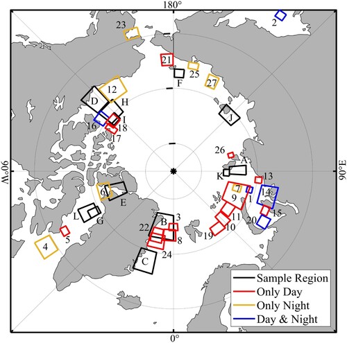
Figure 1. Geolocations of the MODIS images. Regions A∼L represent the 12 sample regions, whereas regions 1∼27 indicate the corresponding evaluation regions.

2.2. NIR sea ice concentration data

To validate the TIR SICs retrieved from MPA and TIRIA, SIC with a finer spatial resolution (250 m) is estimated from the NIR images. Sea ice can be discriminated from open water in the NIR spectrum due to their differences in reflectance (Shokr and Sinha 2023). To mitigate the influence of land and clouds on the ice/water discrimination, we employ land and cloud masks to exclude these pixels, resulting screened images containing only ice and water.

The Otsu method (Otsu 1979) is a classical threshold selection method that identifies threshold values maximizing the between-class variances of a histogram. This method is applicable for thresholding histograms exhibiting bimodal or multimodal distributions. Considering the large variability in sea ice reflectance (Gignac et al. 2017; Ludwig, Spreen, and Pedersen 2020), which leads to a multimodal distribution of reflectance, the single-threshold Otsu method could easily misclassify thin ice with low reflectance as water. To mitigate the classification errors resulting from the high variability in ice reflectance, this study employs a multi-threshold approach instead of a single-threshold. The Otsu method is adapted to derive two thresholds for three surface classes, with only the class exhibiting the lowest reflectance being considered as seawater. Given the substantial presence of high-reflectance ice pixels, which could introduce a positive bias in the Otsu thresholding method, we exclude pixels with reflectance values above 0.3 when determining the threshold. Each NIR image is classified into three classes using the two thresholds derived from the multi-threshold Otsu method. Seawater is classified into the first category due to its lower reflectance, while the other two categories are comprised of various types of ice with higher reflectance.

The binary classification of ice and water at a 250 m resolution is further converted into SIC at resolutions of 1 km and 6.25 km, based on the fraction of ice pixels within the valid pixels (i.e. the total number of ice/water pixels in the coarse pixel with resolutions of 1 km or 6.25 km). To ensure the accuracy of the SIC calculation, coarse pixels with less than 80% valid pixels are excluded.

2.3. Other data

2.3.1. AMSR2 sea ice concentration

The Advanced Microwave Scanning Radiometer 2 (AMSR2) onboard the Global Change Observation Mission-Water Satellite 1 (GCOM-W1) was launched in May 2012. It provides horizontal (H) and vertical (V) polarization brightness temperature data at seven different frequencies (6.9, 7.3, 10.6, 18.7, 23.8, 36.5, and 89 GHz). Brightness temperatures at 89 GHz have the finest spatial resolution and are commonly used for SIC retrieval (Markus and Cavalieri 2000; Spreen, Kaleschke, and Heygster 2008). The Arctic Radiation and Turbulence Interaction Study (ARTIST) Sea Ice Algorithm (ASI) uses a polarization difference of water and ice in 89 GHz to estimate SIC (Beitsch, Kaleschke, and Kern 2014; Spreen, Kaleschke, and Heygster 2008). In this study, the daily SIC dataset retrieved from AMSR2 with ASI algorithm is used to inter-compare with the TIR SIC results. The data are obtained from the University of Bremen (Spreen, Kaleschke, and Heygster 2008), with grid spacing of 6.25 km in polar stereographic projection, covering the period from March 2019 to May 2020.

2.3.2. Subsurface ocean salinity data

To account for the influence of seawater salinity on seawater freezing point, which is crucial for discriminating ice and water, we use EN.4.2.2 subsurface ocean salinity dataset developed by the Met Office Hadley Centre (Good, Martin, and Rayner 2013) in the calculation of TIR SIC. EN.4.2.2 is a subsurface temperature and salinity dataset for the global oceans from 1900 to the present at a monthly timestep. It provides salinity data at 42 layers from depth of 5 m to 5350 m with $1^{\circ }\times 1^{\circ }$ spatial resolution. In this study, only subsurface salinity at a depth of 5 m is used to account for the impact of salinity on seawater freezing point.

2.3.3. Sample data

To obtain the regression coefficients in the Gaussian function of seawater emissivity (see section 3.3), we utilized 16 MODIS images across 12 sample regions to select samples points with varying ice concentrations (regions A∼L in Figure 1 and Table A1). The rules of sample points selection are as follows.

Based on the NIR SICs, pixels with SICs below 100% are selected. Note that fully ice-covered pixels (SIC of 100%) are excluded from the sample points to mitigate the influence of ice. Conversely, pixels with SIC of 0%, located from more than one pixel away from the sea ice area (SIC greater than 0%), are also excluded. This is because seawater emissivity is estimated based on the physical temperature, which is assumed to be equal to the freezing temperature of seawater in the calculation, even though it could be much higher for seawater in the open ocean. The corresponding TIR brightness temperature, sensor zenith angle, salinity of seawater and freezing temperature are extracted accordingly from the sample points. Methods of calculating the TIR ice concentration and freezing temperature of seawater are described in section 3.1 and 3.2, respectively.

3. Methods

3.1. The new thermal infrared ice concentration algorithm (TIRIA)

Instead of surface temperature, TIRIA uses brightness temperature contrast to distinguish open water and sea ice. It assumes that the observational brightness temperature at TIR band ($T{B}_{\mathrm{obs}}$) is linearly weighted by the typical brightness temperature of sea ice ($T{B}_{\mathrm{ice}}$) and brightness temperature of open water at the freezing point ($T{B}_{\mathrm{ow}}$). In TIRIA, SIC is calculated with the following equations: (1) $\mathrm{SIC}=\{\begin{array}{cc}1& \mathrm{if}T{B}_{\mathrm{obs}}\le T{B}_{\mathrm{ice}}\\ {\displaystyle \frac{T{B}_{\mathrm{obs}}-T{B}_{\mathrm{ow}}}{T{B}_{\mathrm{ice}}-T{B}_{\mathrm{ow}}}}& \mathrm{if}T{B}_{\mathrm{ice}}<T{B}_{\mathrm{obs}}<T{B}_{\mathrm{ow}}\\ 0& \mathrm{if}T{B}_{\mathrm{obs}}\ge T{B}_{\mathrm{ow}}\end{array}$(1) The main process of TIRIA includes the following steps: (1) select cloud free pixels, (2) estimate $T{B}_{\mathrm{ice}}$, (3) estimate $T{B}_{\mathrm{ow}}$, (4) calculate SIC.

In the first step, pixels labeled as ‘confident cloudy’ in the cloud mask product are masked out, following the same rules as the MOD29 IST product (Hall and Riggs 2021). Pixels labeled as ‘uncertain clear’, ‘probably clear’ and ‘confident clear’ are assumed to have little influence of clouds thus are kept in the calculation. In the second step, $T{B}_{\mathrm{ice}}$ is estimated similarly as that in MPA (Drüe and Heinemann 2004; Ludwig et al. 2019; 2020). By filling the edge area with NaN (not a number), each TIR image is segmented into 48 × 48-pixel cells (see Figure 2). Each cell is further split into 3 × 3 subcells (each with 16 × 16 pixels). For each subcell, the 25th percentile of the brightness temperature distribution is regarded as the preliminary $T{B}_{\mathrm{ice}}$ ($T{B}_{\mathrm{ice},\mathrm{pre}}$), resulting in 9 $T{B}_{\mathrm{ice},\mathrm{pre}}$ values for each cell. To account for the gradient within the 48 × 48-pixel cell, a linear regression of the x/y position within each cell is performed: (2) $\begin{array}{c}T{B}_{\mathrm{ice}}\left(x,y\right)=\mathrm{ax}+\mathrm{by}+c\end{array}$(2) where x and y are the indices of the respective pixel within the cell, $T{B}_{\mathrm{ice}}\left(x,y\right)$ is the $T{B}_{\mathrm{ice}}$ at the pixel $\left(x,y\right)$, and $\mathrm{a},b,c$ are the regression coefficients.

Figure 2. Schematic diagram for the organization of cells and subcells as well as the moving averaging procedure.

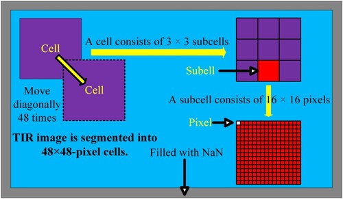
Note that the subcells are considered valid only if more than 30% of the pixels are cloud free, and cells are considered valid only if there are at least five valid subcells. The criteria of defining valid subcell and cell have been confirmed to be reasonable (Drüe and Heinemann 2004; Lindsay and Rothrock 1995). For each valid cell, coefficients $\mathrm{a},b,c$ are determined using the valid subcell preliminary background brightness temperatures ($T{B}_{\mathrm{ice},\mathrm{pre}}$). When coefficients $\mathrm{a},b,c$ are determined, $T{B}_{\mathrm{ice}}\left(x,y\right)$ is calculated using the coefficients of each cell, which may lead to clear boundary patterns between the neighbor cells. To mitigate such problem, a moving average approach has been used in previous studies (Ludwig et al. 2019; 2020). Following the moving average procedure, we shift the cell along the 48 diagonal pixels (48 times) to get 48 estimates of each pixel (see Figure 2). The average of the 48 estimates is regarded as the final $T{B}_{\mathrm{ice}}$.

In the third step, two factors are considered in the estimation of open water brightness temperature at freezing point ($T{B}_{\mathrm{ow}}$): sea salinity and satellite observation angle. The freezing temperature of seawater is affected by sea salinity, while the emissivity of seawater is influenced by satellite observation angle. In the TIR wavelength range, $T{B}_{\mathrm{ow}}$ can be calculated using the following equation: (3) $\begin{array}{c}T{B}_{\mathrm{ow}}={ϵ}_{\mathrm{ow}}^{\frac{1}{4}}\cdot T_{\mathrm{ow}}\end{array}$(3) where ${ϵ}_{\mathrm{ow}}$ is the emissivity of seawater at TIR band, $T_{\mathrm{ow}}$ is the freezing point of seawater. Detailed estimation of these two parameters is introduced in Sections 3.2 and 3.3.

Finally, in the last step, SIC is calculated using Equation (1) for each cloud free pixel of the granule. SIC results retrieved from TIRIA are presented in Section 4.

3.2. Seawater freezing temperature varying with salinity

The freezing temperature of seawater decreases nearly linearly with salinity (Shokr and Sinha 2023). The salinity of seawater in the Arctic differs across regions (see Figure 3(a)). Areas with strong river inflow could have low salinities down to 15‰, while the salinity in the Atlantic Ocean can reach 35‰. A difference in seawater salinity of 20‰ results in a freezing temperature difference of 1.07 K. This difference, which is much larger than the calibration accuracy of brightness temperature (0.05 K for MODIS), could have non-negligible influence on SIC retrieval. The freezing temperature of seawater is calculated as follows: (4) $\begin{array}{c}{T}_{\mathrm{ow}}=-\alpha \cdot S_{\mathrm{ow}}+\text{β}\end{array}$(4) where $\alpha$ and $\text{β}$ are linear coefficients from previous studies (Shokr and Sinha 2023), $S_{\mathrm{ow}}$ is salinity of the sea surface layer.

Figure 3. (a) Salinity of the sea surface layer and (b) Seawater freezing temperature in the Arctic in 2019.

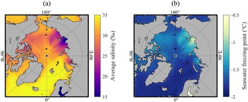
The seasonal variation of salinity in the Arctic is nearly negligible compared with its spatial variation, with temporal and spatial standard deviation of 0.26‰ and 2.79‰, respectively, for the ocean surface salinity data in 2019. We therefore use the annual average salinity in the calculation of seawater freezing temperature. Sea surface salinity and the calculated freezing temperature of the Arctic Ocean and surrounding seas in 2019 are shown in Figure 3(a,b). The highest freezing temperature in the Arctic is found in the Laptev Sea (about −0.5°C), while the lowest freezing temperature is about −1.8°C, with a difference of over 1°C (see Figure 3(b)).

3.3. Sea surface emissivity varying with zenith angle

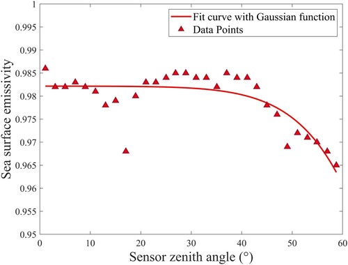
Most of the TIR SIC retrieval algorithms assume that the water surface emissivity is a constant of one or close to one. However, factors such as the view angle of the sensor, wavelength of electromagnetic wave and surface roughness of water (surface wind) impact the emissivity of seawater. Especially at large viewing angles, the TIR sea surface emissivity decreases sharply with the zenith angle (Niclòs et al. 2007). Considering the wide range of viewing angles in TIR images, it is important to account for the angular dependence in the seawater emissivity estimation.

Previous studies have demonstrated that the Gaussian function is effective in capturing the dependence of seawater emissivity on zenith angle (Masuda, Takashima, and Takayama 1988; Niclòs et al. 2005). Therefore, we employ a Gaussian function to establish this relationship and consequently address the influence of observation angle in the ice concentration retrieval. (5) $\begin{array}{c}{ϵ}_{\mathrm{ow}}\left(\theta \right)=y_0+{\displaystyle \frac{A}{\omega \sqrt{0.5\pi }}\exp \left\{-2{\left[{\displaystyle \frac{\theta -{\theta }_c}{\omega }}\right]}^2\right\}}\end{array}$(5) where $\theta$ is the sensor zenith angle, $y_0,A,\omega ,{\theta }_c$ are the regression coefficients. To derive these coefficients, we use sample points as described in Section 2.3.3 and calculate their SICs with TIRIA using varying emissivity. The sample points are grouped within an interval of every 2° of sensor zenith angle (ranging from 0° to 60°) into 30 angular intervals. For each sample point, a set of SICs $\left(\mathrm{SI}{C}_e\right)$ are calculated with emissivity varying between 0.950 and 0.999 (interval of 0.001). When the root mean square error (RMSE) between $\mathrm{SI}{C}_e$ and $\mathrm{SI}{C}_o$ (NIR SIC of the sample point) reaches the minimum, the corresponding emissivity is regarded as the optimal seawater emissivity (${ϵ}_{\mathrm{ow}}$) of that angular interval.

A Gaussian regression of the zenith angle is performed for the seawater emissivity (Figure 4). The derived regression coefficients are as follows: $y_0=0.9822,A=-37.54,$ $\omega =49.15,{\theta }_c=123.6$. RMSE of the regression is 0.004, whereas the R-squared value is 0.64. Based on the regression coefficients and Equation (5), seawater emissivity can be calculated for a given observation angle, and is subsequently used in TIRIA.

Figure 4. Seawater emissivity varying with the sensor zenith angle.

4. Results

Thirty-two MODIS TIR images are used to derive SICs with TIRIA and MPA. These images cover 27 regions of the Arctic (geolocations shown in Figure 1 and Table A2). Among them, 15 regions are covered by daytime-only images, 7 regions by nighttime-only images, and 5 regions have both daytime and nighttime images. To evaluate the two TIR-based SIC retrieval algorithms (TIRIA and MPA), the results are validated with the NIR SICs and inter-compared with the PM SIC product (AMSR2 SIC). Given the potential impact of diurnal variability in ice and water emissivity on performance (Eastwood et al. 2011; Kuenzer and Dech 2013; Nielsen-Englyst et al. 2019), both daytime and nighttime images are analyzed to assess their respective performances.

4.1. Overall accuracy

Twenty daytime NIR images (geolocations shown in Figure 1) are used to validate the TIR SIC results. The NIR and TIR images are both obtained from MODIS thus have the same acquisition time. Therefore, we do not need to consider the time difference between the results and validation datasets, which could sometimes highly influence the validation in highly dynamic sea ice conditions. Bias, RMSE and correlation coefficient ($r$) for the TIR and AMSR2 SICs are summarized in Table 1. For comparative analysis, the evaluation is conducted at resolutions of 1 km and 6.25 km, respectively.

Table 1. The TIR SICs in comparison with the AMSR2 and NIR SICs.

	Scenes	Statistics	MPA	TIRIA	AMSR2
NIR	1 km (N1 = 806017)	Bias (%)	−2.23	−2.86	–
		RMSE (%)	17.63	14.01	–
		$r$	0.81	0.89	–
	6.25 km (N2 = 18429)	Bias (%)	−2.38	−3	−5.28
		RMSE (%)	12.46	8.16	13.3
		$r$	0.87	0.95	0.89
AMSR2 (Day/Night)	Day (N2 = 18835)	Bias (%)	2.9	2.28	–
		RMSE (%)	16.26	13.51	–
		$r$	0.8	0.87	–
	Night (N2 = 13084)	Bias (%)	8.44	5.13	–
		RMSE (%)	23.33	19.02	–
		$r$	0.81	0.87	–
	All (N2 = 31535)	Bias (%)	5.2	3.47	–
		RMSE (%)	19.51	16.03	–
		$r$	0.81	0.87	–

Note: N₁ is the number of pixels with 1 km resolution. N₂ is the number of pixels with 6.25 km resolution.

At 1 km resolution, TIRIA outperforms MPA with its higher correlation (0.89 and 0.81, respectively) and smaller RMSE (14.01% and 17.63%, respectively) though slightly larger bias. Both algorithms tend to underestimate SICs, with the respective bias of −2.86% and −2.23% for TIRIA and MPA. At 6.25 km resolution, the performances of TIRIA and MPA are similar. Both TIR SICs perform better than the AMSR2 SICs, with TIRIA exhibiting the best performance. The underestimation in the AMSR2 SICs is more pronounced than in the TIR SICs.

In addition to the validation with NIR SICs, the SICs derived from the 32 MODIS TIR images are inter-compared with the AMSR2 SICs at 6.25 km resolution to assess their performances during both daytime and nighttime. Statistics for the daytime, nighttime and all MODIS TIR images are presented in Table 1. In comparison, both TIRIA and MPA give generally consistent retrievals with the AMSR2 SICs, albeit with a slight overestimation. TIRIA yields more consistent results than MPA in both daytime and nighttime images, with lower RMSEs and higher correlations (Table 1). This, along with the evaluation results using NIR SICs, indicates the better performance of TIRIA and will be further discussed in Section 4.2. Compared with nighttime images, the daytime TIR SICs deviate less from the AMSR2 SIC, with smaller biases and RMSEs.

To evaluate the performance of the SIC products across various ice distribution conditions, we analyze the statistics at 10% intervals of SIC ranging from 0% to 100% (see Figure 5). Compared to NIR SICs, the TIR SICs are overestimated in the low and mid SIC intervals (SIC below 70%) while underestimated in the high SIC intervals (SIC above 70%). Between the two TIR SICs, TIRIA outperforms MPA in all SIC intervals, with average SICs closer to the NIR SICs in each interval. The largest difference between TIRIA and MPA is found in the 0% SIC interval. In this interval, the average SIC decreases by nearly 15%, and the number of pixels is significantly larger than those between 0% and 90% (Figure 5(b)). The average TIR SIC at the 90–100% interval is nearly identical to the NIR SIC, which indicates the accurate identification of fully ice-covered pixels. While the overestimation in the 0% SIC interval is significantly mitigated in TIRIA, the difference between TIRIA and MPA is nearly negligible in other intervals. This well explains the overall better performance of TIRIA than MPA, yet with slightly larger negative bias (Table 1). The AMSR2 SICs, on the other hand, exhibit underestimations in all the SIC intervals except 0% (Figure 5(c)). Due to the overall underestimation in nearly all the intervals, the AMSR2 SIC has a larger negative bias than the TIR results.

Figure 5. Frequency distributions of two TIR SICs (1 km) and AMSR2 SICs (6.25 km) compared to NIR SICs at 10% intervals of SIC (a-c), along with the two TIR SICs compared with AMSR2 SICs in daytime and nighttime images (d-g).

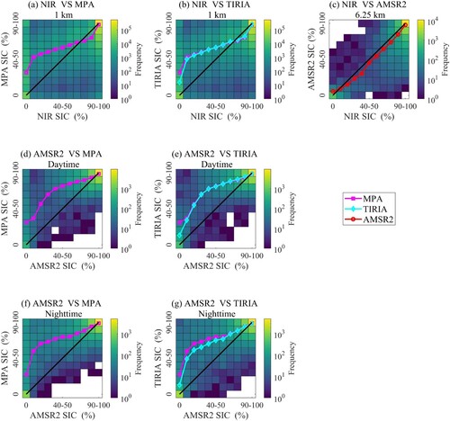
As mentioned above, both daytime and nighttime TIR SICs exhibit overestimations compared to the AMSR2 SICs. The overestimations are found at all the SIC intervals except 90–100% (Figure 5(d–g)). This is expected considering the overall performance of the TIR SICs and AMSR2 SICs compared to the NIR SICs. Between the two TIR SICs, the TIRIA SICs are more consistent with the AMSR2 SICs than the MPA SICs in all the SIC intervals, with generally larger difference in the low SICs.

In addition, differences between the AMSR2 SICs and TIR SICs are larger in the nighttime images than that in the daytime images, especially in low and mid SIC intervals (SIC below 70%). Interestingly, the larger differences align with the smaller number of data points in the these SIC intervals, with an average of less than 300 points per interval. In the 0% intervals of the TIRIA SICs, there are over 1000 data points from the daytime and nighttime images (1025 and 1959, respectively), which results in an average difference of TIRIA SIC less than 1% (e.g. Figure 5(e,g)). For high SIC intervals (SIC above 70%), the number of data points of each interval is more than 800, when the average difference between the daytime and nighttime TIRIA SICs is about 1%. In comparison, the number of data points in the 0–10% SIC interval is 189 and 324, respectively, from daytime and nighttime images. This well corresponds to an average difference of SIC about 15% between the daytime and nighttime cases (respective SIC of 29.39% ad 44.04%). Additionally, for the SICs between 10% and 70%, the average difference is about 4–8% per interval between the daytime and nighttime cases. Such difference is smaller than that in the 0–10% SIC interval, however much higher than that in the 0% and high SIC intervals. Based on the difference of SIC (between the TIR and AMSR2 SICs) in different intervals and the overall overestimation of TIR SICs in low SICs, it can be inferred that the larger difference for nighttime cases is mainly attributed to the larger proportion of data points in the low and mid SIC intervals (2192/13084 and 2305/18835, respectively).

4.2. Case studies

In this section, we select two examples to further investigate the performances of TIRIA and MPA during daytime and nighttime. Both examples are obtained from region 16 (geolocation shown in Figure 1) on May 19th, 2019 (daytime) and May 20th, 2019 (nighttime). The respective SICs and statistics of the evaluation results are presented in Figures 6 (daytime) and 7 (nighttime), and Table 2.

Figure 6. Validation of the TIR and AMSR2 SICs around the Banks Island on 19 May 2019 (region 16 in Figure 1 and Table 2). (a) Reflectance of the MODIS NIR band (band 2); (b) Ice-water binary map from MODIS NIR reflectance; (c) and (j) MODIS NIR SIC at 1 km and 6.25 km resolution; (d) IST of MODIS; (e) MODIS MPA SIC; (f) Differences between MPA and the NIR SIC; (g) TIR brightness temperature of MODIS band 31; (h) MODIS TIRIA SIC; (i) Differences between TIRIA and the NIR SIC; (k) AMSR2 SIC; (l) Differences between the TIRIA, AMSR2 and the NIR SIC.

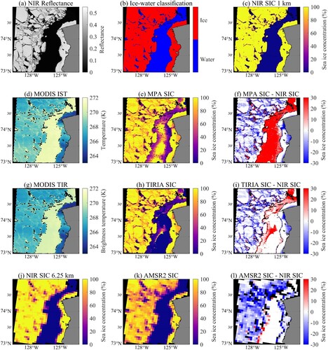
Table 2. TIR SICs in comparison with the NIR and AMSR2 SICs (cases19 and 20).

	Scenes	Statistics	MPA	TIRIA	AMSR2
NIR (case 19)	1 km (N1 = 37750)	Bias (%)	10.99	−1.19	–
		RMSE (%)	35.28	16.62	–
		$r$	0.68	0.93	–
	6.25 km (N2 = 886)	Bias (%)	11.8	−0.90	−8.97
		RMSE (%)	33.31	11.73	16
		$r$	0.72	0.97	0.95
AMSR2	Day (case 19) (N2 = 886)	Bias (%)	20.77	8.06	–
		RMSE (%)	34.77	15.94	–
		$r$	0.73	0.94	–
	Night (case 20) (N2 = 931)	Bias (%)	25.75	7.12	–
		RMSE (%)	39.64	17.02	–
		$r$	0.69	0.93	–

Note: Note: N₁ is the number of pixels with 1 km resolution. N₂ is the number of pixels with 6.25 km resolution.

In the daytime case (case 19, Figure 6 and Table 2), TIRIA outperforms MPA with a significantly smaller bias and higher correlation coefficient. Both TIRIA and MPA tend to underestimate SIC in sea ice area and overestimate it in open water area. As shown in the NIR SICs (Figure 6(c)), most of the open water area in the eastern part of the image is correctly identified by TIRIA but not MPA. The combined effect is the bias of MPA SIC towards larger positive values meanwhile the RMSE being larger. This well explains the overall performance of MPA and TIRIA. In the eastern part of the image, which is open water according to the NIR reflectance, the surface temperature is about 270.9 K according to the IST data. This temperature is lower than the fixed freezing temperature (271.35 K), thus is regarded as ice in MPA and eventually leads to an extensive overestimation of SIC. In TIRIA, brightness temperature is used instead of the IST data. Therefore, the error in the IST data does not impede the identification of open water. In addition, the fixed freezing temperature (273.15 K) is adjusted to the brightness temperature of seawater at freezing temperature, which varies with the seawater salinity. This adjustment enables TIRIA to identify most of the open water. Nevertheless, part of the open water is still misidentified as sea ice in TIRIA (Figure 6(h,i)) due to the low brightness temperatures caused by factors such as clouds. As shown in Figure 6(k), although the PM data could identify large open water area, it is not able to preserve detailed ice distribution information due to the coarse resolution. The overall underestimation of AMSR2 SICs leads to a large bias, and RMSE.

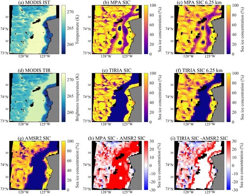
In the nighttime case (case 20, Figure 7 and Table 2), the TIR SICs are compared with the AMSR2 SICs at 6.25 km resolution. Compared with the AMSR2 SICs, the two TIR SICs are generally overestimated, mainly attributed to the overall underestimation of AMSR2 SICs. Between the two TIR SICs, TIRIA manages to identify almost all the open water area (Figure 7(e,f)), whereas MPA identifies very few (Figure 7(b,c)). Along the ice edge, TIRIA detects more ice than the AMSR2 SICs (Figure 7(i)). It is expected that there could be a significant difference between the PM SICs and TIR SICs in the marginal ice zone. This could be attributed to the use of weather filter in AMSR2 SIC, which inaccurately categorizes the low SIC area as open water and leads in marginal ice zone (Lu, Heygster, and Spreen 2018; Spreen, Kaleschke, and Heygster 2008; Wiebe, Heygster, and Markus 2009). In addition, the coarse resolution of PM data and the acquisition time difference between the TIRIA SICs and AMSR2 SICs may also contribute to this discrepancy.

Figure 7. Comparison of the TIR and AMSR2 SICs around the Banks Island on 20 May 2019 (region 16 in Figure 1 and Table 2). (a) IST of MODIS; (b) MODIS MPA SIC; (c) MODIS MPA SIC at 6.25 km resolution; (d) brightness temperature of MODIS band 31; (e) MODIS TIRIA SIC; (f) MODIS TIRIA SIC at 6.25 km resolution; (g) AMSR2 SIC; (h) and (i) Differences between the MPA, TIRIA SICs and the AMSR2 SICs.

5. Discussions

All the current TIR SIC retrieval algorithms are heavily reliant on the surface temperature data, which often introduces additional error in the retrieval process (Hall and Riggs 2021; Shuman et al. 2014). To address this issue, a new retrieval algorithm that does not rely on surface temperature data has been developed, the name of which is TIRIA. In comparison of the two TIR SIC algorithms, performances of the TIR SIC algorithms could be attributed to the following three factors: (1) tie-points of ice and water, (2) main concept of the retrieval algorithm, and (3) the influence of clouds.

In TIRIA, the typical brightness temperature (surface temperature used in MPA) of sea ice and open water ($T{B}_{\mathrm{ice}}$ and $T{B}_{\mathrm{ow}}$), regarded as tie-points in PM-based SIC algorithm, are used as the baselines for the SIC retrieval. As described in Section 3, $T{B}_{\mathrm{ice}}$ is derived similarly as that in MPA. This well corresponds to the similar performance of TIRIA and MPA in the 100% SIC interval (Figure 5). As for the tie-points of open water, the impact of salinity on the seawater freezing point is accounted for additionally in TIRIA. This enables a more accurate identification of open water, which subsequently mitigate the overestimation in low SICs and lead to overall better performance of TIRIA (Table 1).

In terms of the main retrieval concept, TIRIA retains the functional form of MPA, but uses brightness temperature data instead of IST data. The direct use of brightness temperature data helps to circumvent additional errors introduced in the IST inversion process. However, given the similar functional form (and assumption) in TIRIA and MPA, it is expected that they perform similarly in different SIC intervals, showing overestimation in low SICs and underestimation in high SICs (Figure 5).

As illustrated in Section 3, the brightness temperature (or surface temperature in MPA) of each pixel, $T{B}_{\mathrm{obs}}$, is assumed to be linearly weighted by the brightness temperature (or surface temperature in MPA) of ice and water ($T{B}_{\mathrm{ice}}$ and $T{B}_{\mathrm{ow}}$). If the linear assumption holds, the performance of TIRIA and MPA in the low and high SICs should be attributed to an overestimated $T{B}_{\mathrm{ow}}$ together with an underestimated $T{B}_{\mathrm{ice}}$. In addition, the relationship between the TIR SICs and NIR SICs should be linear in theory. The non-linear relationship exhibited in this study (Figure 5) indicates that it is worth to reconsider the relationship between SIC and brightness temperature (or surface temperature). According to the Stefan–Boltzmann law, the emitted radiation from a surface is proportional to the fourth power of its absolute temperature (and also brightness temperature). The development of new TIR SIC algorithm could build upon this.

Last but not least, although the ‘confident cloudy’ pixels are masked out in the SIC calculation, the influence of clouds inevitably remains. The presence of clouds over open water leads to decreases of brightness temperature (and also surface temperature) (Y. Liu, Key, and Wang 2008) The resulted brightness temperature (and surface temperature) could be much lower than that of the freezing seawater, which eventually leads to extensive overestimation of SIC in the open water region (see Figure 6). This highlights that accurate cloud detection is crucial for the application of TIR SIC algorithms. With the trend of merging multiple satellite data to derive a hemispheric high resolution SIC data (Dworak et al. 2021; Ludwig, Spreen, and Pedersen 2020), the accurate cloud detection and TIR SIC retrieval are becoming equally important.

6. Conclusions

In this study, we have developed a new thermal infrared SIC retrieval algorithm, namely TIRIA. Distinguishing itself from traditional TIR SIC algorithms, TIRIA directly utilizes TIR brightness temperatures from TIR imagery, eliminating the dependence on surface temperature data. Furthermore, TIRIA incorporates factors such as seawater salinity and satellite observation angle to accommodate their influence in the SIC calculation. Two sets of TIR SICs are derived using TIRIA and a traditional algorithm, MPA. The results are subsequently compared with PM SICs and validated against simultaneously acquired NIR SICs.

Overall, TIRIA outperforms MPA, with a smaller RMSE (14.01% and 17.63%, respectively) and higher correlation (0.89 and 0.81, respectively). Compared to the NIR SICs, both TIRIA and MPA SICs exhibit overestimation in low SICs and underestimation in high SICs. However, due to its more accurate identification of open water, TIRIA significantly mitigates the overestimation in low SICs. This, in turn, contributes to the overall superior performance of TIRIA, despite a slightly larger negative bias.

In comparison to the PM SICs, both TIR SICs exhibit an overall overestimation. The TIRIA SICs are more consistent with the PM SICs than the MPA SICs. Differences between the TIR SICs and PM SICs are more pronounced in the nighttime images than those in the daytime images. This is consistent with the higher proportion of low and mid SIC data points in the nighttime images. Hence, we believe that SIC retrievals from nighttime images are equally viable as those obtained from daytime images.

As higher resolution TIR satellite data, exemplified by the Thermal Infrared Spectrometer (with a resolution of 30 m) onboard the Sustainable Development Science Satellite 1 (SDGSAT-1) (Qiu, Li, and Guo 2023), continue to advance, the need for an accurate TIR SIC algorithm becomes increasingly crucial. TIRIA, theoretically applicable to any TIR data, demonstrates great potential for future application. For the further development of TIR SIC algorithms, it is recommended to account for the non-linear relationship between SIC and brightness temperature, as well as to incorporate the detection of melt ponds, leads and clouds.

Acknowledgements

The authors would like to express their gratitude to the two anonymous reviewers for their constructive comments and suggestions, which significantly enhanced the quality of the manuscript.

Disclosure statement

No potential conflict of interest was reported by the author(s).

Data availability statement

The data that support the findings of this study are available from the corresponding author, upon reasonable request.

Additional information

Funding

This study was supported by the National Natural Science Foundation of China [grant number 41925027 and 42106225], the Innovation Group Project of Southern Marine Science and Engineering Guangdong Laboratory (Zhuhai) [grant number 311021008], the Natural Science Foundation of Guangdong Province, China [grant number 2022A1515011545], and the CAST Innovation Fund.

Appendix

Tables A1 and A2 are included to show the detailed information, including region, acquisition time and geolocations, of the sample and evaluation MODIS images, respectively.

Table A1. Region, acquisition time and geolocation of the sample MODIS images. All the sample images are obtained in 2019.

Region	Date	Time	LonL (°)	LonR (°)	LatB (°)	LatU (°)
A	0501	0640	87.08	94.69	77	80
B	0502	2030	−21	0	77.5	82
C	0503	1935	−22.58	−11.63	71	75
D	0504	0350	−137.43	−127.85	69	72.85
E	0505	0115	−77.81	−65.14	77.4	80.88
F	0508	0015	174	179.5	71.5	73
G	0515	0150	−65	−60	73	75
	0515	1825
	0515	2000
	0515	2140
H	0519	1940	−140	−128	73	76
	0520	2025
I	0522	2010	−135	−128	75	76.5
J	0522	1150	128.88	141.97	74.66	76.83
K	0525	1400	84.91	91.94	80	81.06
L	0528	0120	−68	−60	71.5	74.59

Table A2. Region, acquisition time and geolocation of the evaluation MODIS images. The images in regions 1∼18 and 19∼27 are obtained from 2019 and 2020, respectively.

Region	Date	Time	LonL (°)	LonR (°)	LatB (°)	LatU (°)
1	0312	0655	74	78.3	75.5	76.5
	0312	1500
2	0327	0120	144.5	147.1	54.8	56.2
	0327	1235
3	0421	1240	−4.58	4.19	79.28	80.53
4	0426	0115	−62.51	−55.52	61.78	64.81
5	0430	1555	−62.86	−59	67.07	68.27
6	0501	0315	−80	−68	76	78.2
7	0501	1805	72.12	77.5	77.53	78.97
8	0502	1400	−9.08	1.83	77.39	79.4
9	0504	0710	60	79	76	80
10	0504	0850	42.1	49	76.5	78.9
11	0504	0850	50	60	77.2	79
12	0504	0705	−150	−138	70	73.3
13	0518	0725	82	86	74.1	75.3
14	0518	0725	69	81	71	74
	0518	1710
15	0519	0630	64	69.2	71.5	72.7
16	0519	1940	−130	−123	73	75
	0520	0705
17	0522	2010	−127	−122.5	75.5	77.5
18	0606	0610	−134	−126	75	76.7
19	0315	0915	32.21	42.1	76.2	77.8
20	0403	0810	57.33	63.46	70.53	72.34
	0403	1615
21	0411	2350	−179.75	−173.86	68.7	70.79
22	0422	1335	−19	−9.53	76.82	79.32
23	0425	0900	−165.98	−160.57	63	64.75
24	0501	1330	−19.46	−7.42	75.74	78.24
25	0508	1010	166.81	172.05	70.03	71.18
26	0511	0550	103.53	107.91	78.88	79.82
27	0512	1125	154	160	71.31	73.5

References

- Andersen, S., R. Tonboe, S. Kern, and H. Schyberg. 2006. “Improved Retrieval of Sea Ice Total Concentration from Spaceborne Passive Microwave Observations Using Numerical Weather Prediction Model Fields: An Intercomparison of Nine Algorithms.” Remote Sensing of Environment 104 (4): 374–392. https://doi.org/10.1016/j.rse.2006.05.013.
- Baldwin, D., M. Tschudi, F. Pacifici, and Y. Liu. 2017. “Validation of Suomi-NPP VIIRS Sea Ice Concentration with Very High-Resolution Satellite and Airborne Camera Imagery.” ISPRS Journal of Photogrammetry and Remote Sensing 130: 122–138. https://doi.org/10.1016/j.isprsjprs.2017.05.018.
- Beitsch, A., L. Kaleschke, and S. Kern. 2014. “Investigating High-Resolution AMSR2 Sea Ice Concentrations During the February 2013 Fracture Event in the Beaufort Sea.” Remote Sensing 6 (5): 3841–3856. https://doi.org/10.3390/rs6053841.
- Cai, Q., J. Wang, D. Beletsky, J. Overland, M. Ikeda, and L. Wan. 2021. “Accelerated Decline of Summer Arctic Sea Ice During 1850–2017 and the Amplified Arctic Warming During the Recent Decades.” Environmental Research Letters 16 (3): 034015. https://doi.org/10.1088/1748-9326/abdb5f.
- Dabboor, M., and T. Geldsetzer. 2014. “Towards Sea Ice Classification Using Simulated RADARSAT Constellation Mission Compact Polarimetric SAR Imagery.” Remote Sensing of Environment 140: 189–195. https://doi.org/10.1016/j.rse.2013.08.035.
- Drüe, C., and G. Heinemann. 2004. “High-Resolution Maps of the Sea-Ice Concentration from MODIS Satellite Data.” Geophysical Research Letters 31 (20): L20403. https://doi.org/10.1029/2004GL020808.
- Dworak, R., Y. Liu, J. Key, and W. N. Meier. 2021. “A Blended Sea Ice Concentration Product from AMSR2 and VIIRS.” Remote Sensing 13 (15): 2982. https://doi.org/10.3390/rs13152982.
- Eastwood, S., P. Le Borgne, S. Péré, and D. Poulter. 2011. “Diurnal Variability in Sea Surface Temperature in the Arctic.” Remote Sensing of Environment 115 (10): 2594–2602. https://doi.org/10.1016/j.rse.2011.05.015.
- Fan, P., X. Pang, X. Zhao, M. Shokr, R. Lei, M. Qu, Q. Ji, and M. Ding. 2020. “Sea ice Surface Temperature Retrieval from Landsat 8/TIRS: Evaluation of Five Methods Against in Situ Temperature Records and MODIS IST in Arctic Region.” Remote Sensing of Environment 248: 111975. https://doi.org/10.1016/j.rse.2020.111975.
- Fraser, A. D., R. A. Massom, and K. J. Michael. 2009. “A Method for Compositing Polar MODIS Satellite Images to Remove Cloud Cover for Landfast Sea-Ice Detection.” IEEE Transactions on Geoscience and Remote Sensing 47 (9): 3272–3282. https://doi.org/10.1109/TGRS.2009.2019726.
- Fraser, A. D., R. A. Massom, K. I. Ohshima, S. Willmes, P. J. Kappes, J. Cartwright, and R. Porter-Smith. 2020. “High-resolution Mapping of Circum-Antarctic Landfast Sea Ice Distribution, 2000–2018.” Earth System Science Data 12 (4): 2987–2999. https://doi.org/10.5194/essd-12-2987-2020.
- Gignac, C., M. Bernier, K. Chokmani, and J. Poulin. 2017. “IceMap250—Automatic 250 m Sea Ice Extent Mapping Using MODIS Data.” Remote Sensing 9 (1): 70. https://doi.org/10.3390/rs9010070.
- Good, S. A., M. J. Martin, and N. A. Rayner. 2013. “EN4: Quality Controlled Ocean Temperature and Salinity Profiles and Monthly Objective Analyses with Uncertainty Estimates.” Journal of Geophysical Research: Oceans 118 (12): 6704–6716. https://doi.org/10.1002/2013JC009067.
- Hall, D. K., and G. Riggs. 2021. “MODIS/Terra Sea Ice Extent 5-Min L2 Swath 1 km, Version 61 [Dataset].” NASA National Snow and Ice Data Center Distributed Active Archive Center. https://doi.org/10.5067/MODIS/MOD29.061.
- Hall, D. K., G. A. Riggs, and V. V. Salomonson. 2001. Algorithm Theoretical Basis Document (ATBD) for the MODIS Snow and Sea Ice-Mapping Algorithms.
- Heuzé, C., L. Zhou, M. Mohrmann, and A. Lemos. 2021. “Spaceborne Infrared Imagery for Early Detection of Weddell Polynya Opening.” The Cryosphere 15 (7): 3401–3421. https://doi.org/10.5194/tc-15-3401-2021.
- Ivanova, N., O. M. Johannessen, L. T. Pedersen, and R. T. Tonboe. 2014. “Retrieval of Arctic Sea Ice Parameters by Satellite Passive Microwave Sensors: A Comparison of Eleven Sea Ice Concentration Algorithms.” IEEE Transactions on Geoscience and Remote Sensing 52 (11): 7233–7246. https://doi.org/10.1109/TGRS.2014.2310136.
- Ivanova, N., L. T. Pedersen, R. T. Tonboe, S. Kern, G. Heygster, T. Lavergne, A. Sørensen, et al. 2015. “Inter-comparison and Evaluation of Sea Ice Algorithms: Towards Further Identification of Challenges and Optimal Approach Using Passive Microwave Observations.” The Cryosphere 9 (5): 1797–1817. https://doi.org/10.5194/tc-9-1797-2015.
- Jenkins, M., and A. Dai. 2021. “The Impact of Sea-Ice Loss on Arctic Climate Feedbacks and Their Role for Arctic Amplification.” Geophysical Research Letters 48 (15): e2021GL094599. https://doi.org/10.1029/2021GL094599.
- Kern, S., T. Lavergne, D. Notz, L. T. Pedersen, R. T. Tonboe, R. Saldo, and A. M. Sørensen. 2019. “Satellite Passive Microwave Sea-Ice Concentration Data Set Intercomparison: Closed Ice and Ship-Based Observations.” The Cryosphere 13 (12): 3261–3307. https://doi.org/10.5194/tc-13-3261-2019.
- Key, J. R., J. B. Collins, C. Fowler, and R. S. Stone. 1997. “High-latitude Surface Temperature Estimates from Thermal Satellite Data.” Remote Sensing of Environment 61 (2): 302–309. https://doi.org/10.1016/S0034-4257(97)89497-7.
- Kuenzer, C., and S. Dech, eds. 2013. Thermal Infrared Remote Sensing: Sensors, Methods, Applications (Vol. 17). Dordrecht: Springer Science+Business Media. https://doi.org/10.1007/978-94-007-6639-6.
- Lindsay, R. W., and D. A. Rothrock. 1995. “Arctic Sea Ice Leads from Advanced Very High Resolution Radiometer Images.” Journal of Geophysical Research: Oceans 100 (C3): 4533–4544. https://doi.org/10.1029/94JC02393.
- Liu, W., and A. Fedorov. 2022. “Interaction Between Arctic Sea Ice and the Atlantic Meridional Overturning Circulation in a Warming Climate.” Climate Dynamics 58 (5): 1811–1827. https://doi.org/10.1007/s00382-021-05993-5.
- Liu, Y., J. Key, and R. Mahoney. 2016. “Sea and Freshwater Ice Concentration from VIIRS on Suomi NPP and the Future JPSS Satellites.” Remote Sensing 8 (6): 523. https://doi.org/10.3390/rs8060523.
- Liu, Y., J. R. Key, and X. Wang. 2008. “The Influence of Changes in Cloud Cover on Recent Surface Temperature Trends in the Arctic.” Journal of Climate 21 (4): 705–715. https://doi.org/10.1175/2007JCLI1681.1.
- Lu, J., G. Heygster, and G. Spreen. 2018. “Atmospheric Correction of Sea Ice Concentration Retrieval for 89 GHz AMSR-E Observations.” IEEE Journal of Selected Topics in Applied Earth Observations and Remote Sensing 11 (5): 1442–1457. https://doi.org/10.1109/JSTARS.2018.2805193.
- Ludwig, V., G. Spreen, C. Haas, L. Istomina, F. Kauker, and D. Murashkin. 2019. “The 2018 North Greenland Polynya Observed by a Newly Introduced Merged Optical and Passive Microwave Sea-Ice Concentration Dataset.” The Cryosphere 13 (7): 2051–2073. https://doi.org/10.5194/tc-13-2051-2019.
- Ludwig, V., G. Spreen, and L. T. Pedersen. 2020. “Evaluation of a New Merged Sea-Ice Concentration Dataset at 1 km Resolution from Thermal Infrared and Passive Microwave Satellite Data in the Arctic.” Remote Sensing 12 (19): 3183. https://doi.org/10.3390/rs12193183.
- Markus, T., and D. J. Cavalieri. 2000. “An Enhancement of the NASA Team Sea Ice Algorithm.” IEEE Transactions on Geoscience and Remote Sensing 38 (3): 1387–1398. https://doi.org/10.1109/36.843033.
- Masuda, K., T. Takashima, and Y. Takayama. 1988. “Emissivity of Pure and Sea Waters for the Model Sea Surface in the Infrared Window Regions.” Remote Sensing of Environment 24 (2): 313–329. https://doi.org/10.1016/0034-4257(88)90032-6.
- Niclòs, R., V. Caselles, C. Coll, and E. Valor. 2007. “Determination of Sea Surface Temperature at Large Observation Angles Using an Angular and Emissivity-Dependent Split-Window Equation.” Remote Sensing of Environment 111 (1): 107–121. https://doi.org/10.1016/j.rse.2007.03.014.
- Niclòs, R., E. Valor, V. Caselles, C. Coll, and J. M. Sánchez. 2005. “In Situ Angular Measurements of Thermal Infrared Sea Surface Emissivity—Validation of Models.” Remote Sensing of Environment 94 (1): 83–93. https://doi.org/10.1016/j.rse.2004.09.002.
- Nielsen-Englyst, P., J. L. Høyer, K. S. Madsen, R. Tonboe, G. Dybkjær, and E. Alerskans. 2019. “In Situ Observed Relationships Between Snow and Ice Surface Skin Temperatures and 2 m Air Temperatures in the Arctic.” The Cryosphere 13 (3): 1005–1024. https://doi.org/10.5194/tc-13-1005-2019.
- Otsu, N. 1979. “A Threshold Selection Method from Gray-Level Histograms.” IEEE Transactions on Systems, Man, and Cybernetics 9 (1): 62–66. https://doi.org/10.1109/TSMC.1979.4310076.
- Paul, S., and M. Huntemann. 2021. “Improved Machine-Learning-Based Open-Water–Sea-Ice–Cloud Discrimination Over Wintertime Antarctic Sea Ice Using MODIS Thermal-Infrared Imagery.” The Cryosphere 15 (3): 1551–1565. https://doi.org/10.5194/tc-15-1551-2021.
- Paul, S., S. Willmes, and G. Heinemann. 2015. “Long-term Coastal-Polynya Dynamics in the Southern Weddell Sea from MODIS Thermal-Infrared Imagery.” The Cryosphere 9 (6): 2027–2041. https://doi.org/10.5194/tc-9-2027-2015.
- Poliyapram, V., N. Imamoglu, and R. Nakamura. 2019. “Deep Learning Model for Water/Ice/Land Classification Using Large-Scale Medium Resolution Satellite Images.” IGARSS 2019 – 2019 IEEE International Geoscience and Remote Sensing Symposium, Yokohama, Japan, 3884–3887. IEEE. https://doi.org/10.1109/IGARSS.2019.8900323.
- Qiu, Y., X.-M. Li, and H. Guo. 2023. “Spaceborne Thermal Infrared Observations of Arctic Sea Ice Leads at 30 m Resolution.” The Cryosphere 17 (7): 2829–2849. https://doi.org/10.5194/tc-17-2829-2023.
- Qu, M., X. Pang, X. Zhao, R. Lei, Q. Ji, Y. Liu, and Y. Chen. 2021. “Spring Leads in the Beaufort Sea and its Interannual Trend Using Terra/MODIS Thermal Imagery.” Remote Sensing of Environment 256: 112342. https://doi.org/10.1016/j.rse.2021.112342.
- Reiser, F., S. Willmes, and G. Heinemann. 2020. “A New Algorithm for Daily Sea Ice Lead Identification in the Arctic and Antarctic Winter from Thermal-Infrared Satellite Imagery.” Remote Sensing 12 (12): 1957. https://doi.org/10.3390/rs12121957.
- Ren, H., M. Shokr, X. Li, Z. Zhang, F. Hui, and X. Cheng. 2022. “Estimation of Sea Ice Production in the North Water Polynya Based on Ice Arch Duration in Winter During 2006–2019.” Journal of Geophysical Research: Oceans 127 (10): e2022JC018764. https://doi.org/10.1029/2022JC018764.
- Savidge, E., T. Snow, and M. R. Siegfried. 2023. “Multi-Decadal Record of Sensible-Heat Polynya Variability from Satellite Optical and Thermal Imagery at Pine Island Glacier, West Antarctica.” Geophysical Research Letters 50 (22): e2023G–L106178. https://doi.org/10.1029/2023GL106178.
- Shi, W., S. Yuan, C. Liu, Y. Ma, N. Xu, and X. Lv. 2022. “Inversion of Sea Ice Concentration in the Liaodong Bay from MODIS Data.” Remote Sensing 14 (18): 4439. https://doi.org/10.3390/rs14184439.
- Shokr, M., and N. K. Sinha. 2023. Sea Ice: Physics and Remote Sensing. Hoboken, NJ: John Wiley & Sons.
- Shuman, C. A., D. K. Hall, N. E. DiGirolamo, T. K. Mefford, and M. J. Schnaubelt. 2014. “Comparison of Near-Surface Air Temperatures and MODIS Ice-Surface Temperatures at Summit, Greenland (2008–13).” Journal of Applied Meteorology and Climatology 53 (9): 2171–2180. https://doi.org/10.1175/JAMC-D-14-0023.1.
- Spreen, G., L. Kaleschke, and G. Heygster. 2008. “Sea ice Remote Sensing Using AMSR-E 89-GHz Channels.” Journal of Geophysical Research: Oceans 113 (C2): C02S03.
- Sun, Y., Y. Ye, S. Wang, C. Liu, Z. Chen, and X. Cheng. 2023. “Evaluation of the AMSR2 Ice Extent at the Arctic Sea Ice Edge Using an SAR-Based Ice Extent Product.” IEEE Transactions on Geoscience and Remote Sensing 61: 1–15. https://doi.org/10.1109/TGRS.2023.3281594.
- Wang, Q., M. Shokr, S. Chen, Z. Zheng, X. Cheng, and F. Hui. 2022. “Winter Sea-Ice Lead Detection in Arctic Using FY-3D MERSI-II Data.” IEEE Geoscience and Remote Sensing Letters 19: 1–5. https://doi.org/10.1109/LGRS.2022.3223689.
- Wiebe, H., G. Heygster, and T. Markus. 2009. “Comparison of the ASI Ice Concentration Algorithm with Landsat-7 ETM+ and SAR Imagery.” IEEE Transactions on Geoscience and Remote Sensing 47 (9): 3008–3015. https://doi.org/10.1109/TGRS.2009.2026367.
- Willmes, S., and G. Heinemann. 2016. “Sea-Ice Wintertime Lead Frequencies and Regional Characteristics in the Arctic, 2003–2015.” Remote Sensing 8 (1): 4. https://doi.org/10.3390/rs8010004.