RTGDC: a real-time ingestion and processing approach in geospatial data cube for digital twin of earth

ABSTRACT

The emergence of the Digital Twin of Earth (DTE) signifies a pivotal advancement in the field of the Digital Earth, which includes observations, simulations, and predictions regarding the state of the Earth system and its temporal evolution. While the Geospatial Data Cubes (GDCs) hold promise in probing the DTE across time, existing GDC approaches are not well-suited for real-time data ingestion and processing. This paper proposes the design and implementation of a real-time ingestion and processing approach in Geospatial Data Cube (RTGDC), achieved by ingesting real-time observation streams into data cubes. The methodology employs a publish/subscribe model for efficient observation ingestion. To optimize observation processing within the data cube, a distributed streaming computing framework is utilized in the implementation of the RTGDC. This approach significantly enhances the real-time capabilities of GDCs, providing an efficient solution that brings the realization of the DTE concept within closer reach. In RTGDC, two cases involving local and global scales were implemented, and their real-time performance was evaluated based on latency, throughput, and parallel efficiency.

KEYWORDS:

• Data cube
• stream computing
• digital twin of earth
• geospatial big data
• observation

1. Introduction

With the progress in computational science and the growing volume of datasets, computer modeling, data-intensive analysis, and artificial intelligence have become essential elements in numerous Earth science research projects (Bergen et al. 2019; Wang et al. 2021). The ultimate objective of the Digital Earth is to create a Digital Twin of Earth (DTE) (DeFelipe et al. 2022). The DTE aims to digitize different aspects of the Earth system, covering geography, climate, environment, and human society, to attain a detailed and realistic simulation of the Earth. This process entails mapping real-world Earth systems into a virtual digital environment, allowing us to observe, analyze, and predict events within the Earth system with precision and real-time capability (Hoffmann et al. 2023; Oza et al. 2021; Voosen 2020).

Recent advancements in the Geospatial Data Cube (GDC) show promise in supporting the DTE (Gettelman et al. 2022). The GDC is an emerging form of the Spatial Data Infrastructure (SDI) that has garnered increasing attention from institutions such as the Committee on Earth Observation Satellites (CEOS) (Killough 2018), the European Space Agency (ESA) (Mahecha et al. 2020), and the Open Geospatial Consortium (OGC) (Jacovella-St-Louis 2022). GDC, functioning as a multidimensional data model, is employed for efficiently organizing and storing multidimensional geospatial data. It exhibits a unique advantage in supporting the storage and computation of large-scale, heterogeneous geospatial data from various sources, making a substantial contribution to realizing the Digital Earth.

In recent years, the GDC has experienced rapid development, leading to the emergence of numerous practical applications and implementation solutions (Gao et al. 2022; Lewis et al. 2016; 2017; Mahecha et al. 2020; Schleidt and Jetschny 2023a; Schramm et al. 2021). Additionally, it is evolving to achieve greater interoperability. OGC has formed GeoDataCube Standards Working Group (GDC SWG), the goal of which is to facilitate the handling of different GDCs via a Standardized API that will serve the core functionalities of GDCs. However, due to its relatively short history, current GDC implementations mainly operate in batch processing modes and do not yet support the real-time ingestion and processing of observations.

The paper introduces a real-time ingestion and processing approach in Geospatial Data Cube (RTGDC) designed to facilitate the real-time ingestion and processing of large volumes of observations and streams. The main contributions of this article are summarized as follows:

• It seamlessly integrates a Pub/Sub (publish/subscribe) model with the GDC, enabling real-time cube construction and computation.

• It utilizes a stream-based distributed processing framework to enhance the real-time capabilities of the GDC.

• It offers an efficient solution, bringing the realization of the DTE concept closer to reality.

Moreover, a prototype system is developed to demonstrate the feasibility of the approach. The system is evaluated in both local and global scenarios. The local scenario involves the digital twin of Singapore, while the global scenario focuses on global-scale climate analysis. In both cases, the proposed RTGDC demonstrates low latency and accurate simulation and emulation of the DTE.

2 Background and related work

2.1 Digital earth

The Digital Earth is described as a virtual globe constructed of massive, multiresolution, multitemporal, multityped Earth observation data and socioeconomic data combined with the relevant analysis algorithms and models (Goodchild 2013; Grossner, Goodchild, and Clarke 2008; Guo, Goodchild, and Annoni 2020). In its early stages, the Digital Earth primarily focused on data-driven modeling and visualization, making use of existing geographic, environmental, and social data sources. Notable examples encompass Google Earth, ArcGIS Explorer (Kienberger and Tiede 2008), GeoGlobe (Gong et al. 2011), and DESP/CAS (Guo, Fan, and Wang 2009).

With the rapid growth of geospatial data, challenges arose in managing diverse data sources and the computational capacity needed for data-intensive analysis (Goodchild et al. 2012; Guo et al. 2017). Consequently, the emergence of computation-driven Digital Earth platforms became apparent, illustrated by platforms like Google Earth Engine (GEE, https://earthengine.google.com/) (Gorelick et al. 2017), AI Earth Science Cloud Platform (https://engine-aiearth.aliyun.com/), and PIE Engine (https://engine.piesat.cn), among others. For instance, GEE is a robust cloud computing platform introduced by Google, specifically designed to facilitate global-scale Earth observation data analysis. GEE provides petabyte-level publicly accessible remote sensing imagery and other ready-to-use products, along with high-performance distributed computing resources for tasks like remote sensing data processing, time-series analysis, and large-scale image processing (Amani et al. 2020; Gorelick et al. 2017; Tamiminia et al. 2020).

The next phase in the evolution of the Digital Earth is the DTE, an information system presenting users with a digital replica of the Earth system's state and temporal evolution, constrained by available observations and physical laws (Bauer, Stevens, and Hazeleger 2021). This digital twin architecture marks a significant advancement in Earth system modeling, enabling simulations and observations at larger spatial scales and predictions over temporal scales spanning decades (Li et al. 2023).

The European Destination Earth (DestinE) program aims to create a digital twin of the Earth system by 2030. The DestinE initiative seeks to facilitate a wide range of decision-making processes, encompassing climate change adaptation, management of extreme weather-related disasters, and similar endeavors (Hoffmann et al. 2023; Voosen 2020). Additionally, the National Aeronautics and Space Administration (NASA) has initiated a mission to develop the Earth System Digital Twins (ESDT), described as interactive, comprehensive, multi-domain, multi-scale digital replicas of the Earth system (Huang et al. 2022; Oza et al. 2021).

In summary, the DTE marks an advanced stage in the development of the Digital Earth, employing digital technologies to construct a comprehensive Earth model. This concept is continuously evolving and maturing, making a profound impact on the field of Earth sciences.

2.2. Geospatial data cube

The concept of the data cube originates from the fields of data warehousing and business intelligence (Abelló et al. 2013; Cody et al. 2002; Cristescu 2017). As a multidimensional data model and structure, the data cube is employed to organize large datasets and facilitate efficient multidimensional data analysis and querying. Building upon the foundation of the data cube, the GDC has emerged as a significant solution for research and applications in the field of Digital Earth.

OGC provides the definitions of the data cube and GDC (Jacovella-St-Louis 2022). A data cube is a multi-dimensional (‘n-D’) array of values (Percivall 2020), and persistently stores and provides efficient access to multi-dimensional information. A GDC is a data cube for which some dimensions are geospatial in nature (such as latitude and longitude, projected easting and northing, or elevation above the WGS84 ellipsoid). In terms of functionality, a GDC can be considered a multi-dimensional field including spatial dimensions, and often temporal dimensions as well.

Table 1 presents a comparison of five typical GDCs and the proposed RTGDC. The EarthServer data cube (Baumann et al. 2016) is built around the high-performance Rasdaman array database (http://www.rasdaman.org) (Baumann et al. 1998; 1999) and adopts OGC Web Coverage Service (WCS) and Web Coverage Processing Service (WCPS) Standards, enhancing service interaction. Rasdaman enables EarthServer to integrate data/metadata retrieval, achieving the same level of search, filtering, and extraction convenience as typical metadata. EarthServer extends the platform into a comprehensive coverage analysis engine, supporting multi-dimensional spatiotemporal coverage through the Web Map Service (WMS)/WCS/WCPS suite, and has integrated data and metadata search.

Table 1. Comparison of different GDCs and the proposed RTGDC.

	EarthServer	AGDC/ODC	ESDC	openEO	GeoCube	RTGDC
Time	2016	2018	2019	2021	2022	2024
Data Source	Raster	Raster	Raster	Raster	Raster/Vector	Raster/Vector
OLAP	No	No	Customized	Customized	Spatial	Observation
Computing Pattern	HPC^1/Batch	HPC/Batch	HPC/Batch	HPC/Batch	HPC/Batch	HPC/Streaming
Data Organization	Raster Tile	Raster Tile/Image	Raster Tile	Raster Tile	Raster Tile/Vector Tile	Raster Tile/Vector Tile
Data Storage	Array Database	NetCDF	Zarr	Format Agnostic	HBase	COG^2/HBase
Metadata	PostgreSQL/SQLite (GMLCOV^3 model)	PostgreSQL (JSONB)	File System (config file)	Meta-database	PostgreSQL	PostgreSQL
User Interface	OGC WCS/OGC WCPS/RaSQL^4	OGC WCS/OGC WPS^5/OGC WMS/Jupyter Notebook	FTP^6/OGC WCS/Jupyter Notebook	openEO API/UDF	OGC API – Coverages/Processes/OGC DAPA^7/Jupyter Notebook	OGC SensorThings API/OGC API – Coverages/Processes
Programming Language	C++/Java/R/ JavaScript	Python	Python/Julia/R	Python/R/JavaScript	Scala/Python	Scala/Python

¹ High Performance Computation (HPC).

² Cloud Optimized GeoTIFF (COG).

³ OGC Geography Markup Language Coverages (GMLCOV).

⁴ Rasdaman Query Language (RaSQL).

⁵ OGC Web Processing Service (WPS).

⁶ File Transfer Protocol (FTP).

⁷ Data Access and Processing API (DAPA).

The Australian Geoscience Data Cube (AGDC) has undergone two major versions. The AGDCv1 (Lewis et al. 2016) utilized high-performance computing and storage resources to process a substantial amount of Landsat data, achieving remarkable breakthroughs in spatial dimensions. The AGDCv2 (Lewis et al. 2017), building upon the AGDCv1, underwent multiple iterations, offering a rigorous definition of spatial and temporal dimensions. It is equipped to support extensive spatial computations and time-series analysis, and offers a more comprehensive dataset spanning various fields such as Earth science, hydrology, climate, ecology, and astronomy. After June 2016, AGDC is known as the Digital Earth Australia (DEA), which is a big data platform that supports the exploitation of Earth observations from space (EOS) and other geospatial data to provide insights into Australia’s changing land, coasts and oceans (Dhu et al. 2017). Furthermore, The CEOS introduced the Open Data Cube (ODC) initiative, based on the AGDC, with the intension of providing free-access development tools for data cubes. This initiative has been successfully implemented in various countries, including Australia and Switzerland (Killough 2018).

ESA proposed the Earth System Data Cube (ESDC) (Mahecha et al. 2020), which emphasizes the adherence to the Findability, Accessibility, Interoperability, and Reusability (FAIR) principles (Wilkinson et al. 2016) and unifies data under a common data model and coordinate reference system. The ESDC centers around a single data stream, incorporating multiple dimensions, such as spatial, temporal, and variables, providing a clear mathematical framework. openEO (https://openeo.org/), an open-source framework for processing Earth observation data, provides standardized interfaces enabling users to consistently access and process Earth observation data consistently, including data cubes (Schramm et al. 2021). Users can construct virtual data cubes and perform computations using User-defined Functions (UDFs). The core objective of FAIRiCUBE (Schleidt and Jetschny 2023a) is to establish a cross-disciplinary platform for the fair and trustworthy ingestion, provision, analysis, processing, and sharing of data, extending beyond traditional Earth observation domains.

GeoCube (Gao et al. 2022) distinguishes itself by seamlessly integrating multiple heterogeneous data sources, encompassing both raster and vector data, within the GDC framework. It makes use of Apache Spark for data computations and explores optimization methods based on machine learning. This enables feature selection and modeling in the geospatial domain, ultimately achieving computational load balancing. Furthermore, GeoCube has implemented Spatial OLAP (SOLAP) on top of Online Analytical Processing (OLAP). Spatial Online Analytical Processing (SOLAP) is a widely used tool for geospatial data mining, allowing for efficient exploration of data cubes to extract new insights (Rivest et al. 2003; 2005). Furthermore, SOLAP facilitates rapid and straightforward spatial and temporal analysis through multidimensional approaches (Han, Stefanovic, and Koperski 1998). Through SOLAP, one can dynamically rearrange, focus, and filter geospatial data using operations such as rolling up, drilling down, slicing, and dicing, especially in the spatial dimension and measure (Bimonte et al. 2014; Li et al. 2014).

In conclusion, data cubes in the Digital Earth domain continually evolve, serving as powerful tools for integrating diverse data sources and conducting multidimensional data analysis. This paper extends the GeoCube framework, enabling the real-time integration of observations and streams into GDCs and facilitating real-time computation. This extension aims to achieve real-time simulation and emulation of the Digital Earth, thereby constructing a DTE.

2.3. Real-time geoprocessing

With the development of infrastructure and innovations in data collection devices, real-time geospatial data has been continuously generated in recent years, gradually becoming an integral component of geospatial data (Li et al. 2016; Rathore et al. 2015; Silva and Holanda 2022). Real-time geographic data refers to data generated continuously, at high frequency, and in real-time on the geographic space, typically involving location, time, and other geographic attributes (Li, Liu, and Wang 2022).

Major sources of real-time geospatial data include sensor networks (Bhattacharya and Painho 2017; Chen et al. 2015; Li and Fu 2011, 2014; Zhai, Yue, and Zhang 2016), mobile devices (Pires et al. 2016), social media platforms (Kulkarni et al. 2015; Rajarathinam, Bhuvaneswari, and Jothi 2022), the Internet of Things (Mohammadi et al. 2018; Tu et al. 2020), and observation networks (Albergel et al. 2015; Zhang et al. 2018). Widely available real-time geospatial data exhibits characteristics of massive volume, multiple sources, and heterogeneity, ultimately leading to a new paradigm for the organization, computation, and programming of real-time geospatial data (Armstrong, Wang, and Zhang 2019; Li, Liu, and Wang 2022).

The Pub/Sub model, with its characteristics of decoupling, asynchronous communication, and scalability, has been widely applied in the transmission of real-time geospatial data (Lazidis, Tsakos, and Petrakis 2022; Livaja et al. 2022; Sun et al. 2016). It has two primary parties: a Publisher that is publishing information and a Subscriber that is interested in all or part of the published information. Also, the topic serves to define the subject or category of messages, where publishers publish messages to specific topics, and subscribers subscribe to topics of interest to receive relevant messages (Braeckel, Bigagli, and Echterhoff 2016; Eugster et al. 2003).

As for real-time data processing, two representative models have gradually emerged: the data stream processing (DSP) model and the complex event processing (CEP) model (Cardellini et al. 2022; Cugola and Margara 2012; Fragkoulis et al. 2023).

Among DSP frameworks, mature options include Apache Storm (Iqbal and Soomro 2015), Apache Spark Streaming (Salloum et al. 2016), and Apache Flink (Carbone et al. 2015). In terms of latency, throughput, complexity, and scalability, they each have their own strengths and weaknesses, making it difficult to determine a clear winner (Isah et al. 2019). Furthermore, there are mainly two DSP architectures, namely Lambda and Kappa. The Lambda architecture mixes the benefit of processing models, batch processing and real-time processing to provide better results in low latency, but maintaining two different sets of code leads to more complexity (Kiran et al. 2015). Kappa is a simplification of lambda architecture which means it’s like a Lambda Architecture system with the batch processing system removed, permitting users to develop, test, debug and operate their systems on top of a single processing framework (Soumaya et al. 2017).

CEP systems efficiently handle large data streams to promptly identify significant occurrences. Events are typically singular instances of interest over time, while complex events represent situations or patterns that hold specific composite significance within the system. Primitive events, which are atomic events, flow into the CEP system, while composite (or complex) events are extracted by the system through defined patterns (rules) involving other raw or additional content (Flouris et al. 2017). This model treats flowing information items as notifications of events in the external world, requiring filtration and composition to understand more advanced events (Cugola and Margara 2012). The geospatial complex event processing integrates spatial attributes into event definitions and reasoning rules, can enhance smart city systems’ ability to detect and analyze complex events in urban areas (Khazael, Asl, and Malazi 2023).

2.4. Motivation

The DTE aims to monitor, simulate, and predict Earth systems, facilitating bidirectional communication, dynamic interaction, and real-time connectivity between the physical and digital worlds (Li et al. 2023). It necessitates the comprehensive integration of observation data and Earth system models to ultimately establish a knowledge repository guiding human society. Furthermore, the DTE must integrate the human dimension of the Earth system, covering diverse fields such as economics, energy, and agriculture. It should address multidimensional questions such as the economic impact of carbon neutrality on specific regions and industries, as well as the policy orientation of climate change on agricultural management (Bauer, Stevens, and Hazeleger 2021).

Therefore, in a comprehensive perspective, the DTE is poised to more accurately reflect the real-time state of the Earth system by promptly acquiring and effectively analyzing real-time geospatial data. Moreover, a real-time paradigm should be instituted within the DTE to ensure the low-latency utilization of real-time data, tapping into its crucial value – a fact that appears to be overlooked in the current development of the DTE.

As a crucial realization of the DTE, the GDC has made significant contributions, including Earth observation (EO) data management, analysis, services, and interoperability (Annoni et al. 2023; Baumann 2018; Gao et al. 2022; Hamdani et al. 2023; Masmoudi et al. 2021; Mišev et al. 2019; Sudmanns et al. 2023). However, the GDC's real-time connection and dynamic interaction with the physical world still lack systematic proposals and implementions.

Hence, designing and implementing an RTGDC can tackle the following challenges in the DTE:

1. Ensuring real-time capability: By integrating the Pub/Sub model into the GDC, data can be used with low latency, ensuring real-time production and consumption. Additionally, modeling observations and observation streams from the physical world enables the conceptual and logical modeling of the DTE's simulation.

2. Addressing the ‘curse of dimensionality’ caused by a massive number of dimensions: As mentioned earlier, the DTE necessitates integrating observation data and human dimensions, leading to a large volume of data from diverse sources with numerous dimensions. An RTGDC, through the advantages of the GDC, can accomplish the unified integration of multidimensional data. Additionally, indexing all data by dimensions enhances retrieval efficiency.

3. Spatiotemporal analysis and prediction: Drawing on the expertise and contributions of the SOLAP, the RTGDC defines the Observation OLAP mathematically, providing multidimensional spatiotemporal analysis operations. In addition to the OLAP, atomic analysis operators can form a workflow to provide analytical capabilities.

3. Materials and methods

3.1. RTGDC modeling

The GDC and the RTGDC differ fundamentally in data storage frequency and computational paradigm, as illustrated in Figure 1. In the GDC context, it is customary to proactively construct these cubes based on specific data requirements to facilitate subsequent batch processing. In this scenario, the data within the cubes are inherently non-real-time and undergo periodic updates at longer intervals. Users access cube results by submitting batch tasks, characterizing the computational paradigm in this context as batch processing, associated with high latency and initiated by user-driven actions.

Figure 1. The paradigm shift between GDC and RTGDC.

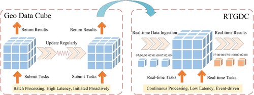
Conversely, the RTGDC computation tasks exhibit characteristics of continuous processing, low latency, and event-driven triggers. Continuous streams of data are fed into the system by the real-time data ingestion approach, facilitating the real-time construction of data cubes. Subsequently, the advantages of real-time data cubes are harnessed for real-time analysis and computation. In such cases, all analytical processes must be initiated via predefined real-time tasks.

The RTGDC primarily models observations and observation streams. A key consideration in modeling was to improve the interoperability of the RTGDC in real-time scenarios by aligning it with existing standard concepts for widespread use. In the context of the OGC/ISO Observations, measurements and samples Standard (ISO 19156:2023 2023; Schleidt and Rinne 2023b), Observation represents the concept of collecting, monitoring or measuring data related to specific features of interest within the real world. Specifically, an Observation refers to data acquired through sensors, instruments, or devices, and is used to describe, record, and represent the state, properties, or characteristics of a particular feature of interest during a specific time point or time interval. The concept of ObservationStream is derived from the OGC SensorThings API (Liang, Khalafbeigi, and van der Schaaf 2021). An ObservationStream is used to represent the real-time, continuous generation of sensor data. ObservationStreams group Observations that measure the same observed property and are generated by the same sensor. It signifies a collection of sensor Observations forming a continuous time series.

Figures 2 and 3 illustrate the conceptual and logical models of the RTGDC respectively. In the physical world, various sensors such as cameras, in-situ stations, drones, and satellites generate Observations, which are aggregated into ObservationStreams. These ObservationStreams are then transmitted in real-time to the RTGDC via the data delivery model (Section 3.2). During the transmission process, observation topics can be predefined to further categorize the ObservationStreams. Different topics enables the categorization of data for publishing and subscribing, facilitating decoupling between publishers and subscribers, thus meeting diverse requirements for constructing and analyzing the RTGDC across various scenarios.

Figure 2. The conceptual model of the RTGDC.

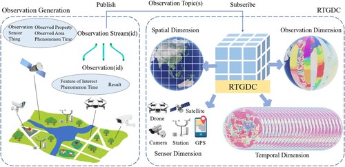
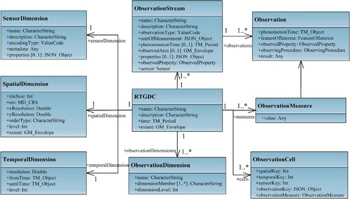
Figure 3. The logical model of the RTGDC.

The distinctions among these concepts are: Observation represents individual data collected mainly by sensors, ObservationStream groups continuous streams of Observations (like sensor data) measuring the same property, while the RTGDC, is a conceptual model that organizes and stores observation data in a multidimensional structure, facilitating efficient management and analysis of Observations for various applications.

This paper defines four dimensions for the RTGDC: spatial dimension, temporal dimension, sensor dimension and observation dimension.

The SpatialDimension is an intrinsic dimension of the RTGDC, defined based on the spatial attributes of the measurements within the cube. It can be considered an indexing structure within the spatial domain. Typically, creating spatial dimension involves subdividing space based on a certain pattern and applying indexing methods (such as the Z-order curve, Hilbert curve, etc.) to establish the spatial dimension. Common global partitioning schemes include Geohash, Google S2, and the OGC Discrete Global Grid Systems (DGGS) (Mahdavi-Amiri, Alderson, and Samavati 2015; Purss and Jacovella-St-Louis 2021), among others.

The TemporalDimension is another inherent dimension within the RTGDC, defined based on the temporal attributes of the measurements in the cube. Each level of the temporal dimension is uniquely determined by its start time, end time, and temporal resolution, and each dimension member is uniquely identified with chronological order. In a real-time cube, recognizing the significance of the temporal dimension, in addition to the fixed-level temporal dimension, a tilted temporal dimension can be defined. In a tilted temporal dimension, level-related time windows can be established, such as 1 min, 1 h, and 1 d. The closer to the current moment, the finer the temporal granularity for stored data.

The SensorDimension is used to indicate the sensor responsible for generating the observational data. This dimension encapsulates the provenance attributes of the observation data, enabling data queries or subsets along the sensor dimension using sensor names.

The ObservationDimension is defined as a dimension for observations that encompasses attributes beyond spatial and temporal properties, reflecting the non-spatiotemporal attributes of observation measures. For instance, in the context of meteorological data, the observation dimension comprises factors such as product dimension (pertaining to the type of meteorological data product), variable dimension (indicating specific variables within the meteorological data product, e.g. wind speed, atmospheric pressure, temperature, etc.), and quality dimension (assessing the quality of meteorological data).

The ObservationMeasure, representing the data to be analyzed within observations, can take various forms, including raster data, vector data, and more.

The ObservationCell, the smallest entity within the RTGDC, serves as the fundamental building block for the entire RTGDC. Additionally, the observation cell serves as the foundational unit for analytical functions within the RTGDC, enabling advanced analyses through operations like filtering, aggregation, and more.

3.2. Observation ingestion

In 2021, OGC published version 1.1 of the OGC SensorThings API Standard to promote the interoperability of geospatial and Internet of Things (IoT) data. This standard employs a RESTful architecture, utilizes HTTP (HyperText Transfer Protocol), and extends to the MQTT (Message Queuing Telemetry Transport) protocol. It defines crucial concepts and entities related to data management, such as Things, Sensors, Observations, and Datastreams, and provides extended capabilities for filtering, creating, updating, and deleting observation results. Furthermore, in 2016, OGC introduced the OGC Pub/Sub (Publish/Subscribe) interface Standard (Braeckel, Bigagli, and Echterhoff 2016) to support the real-time delivery and interaction of geospatial data, offering an interoperable way to publish, subscribe to, and exchange geospatial data.

This study integrates the OGC SensorThings API and OGC Pub/Sub interface standards to implement a Pub/Sub data delivery model for the RTGDC. The specific workflow is illustrated in Figure 4.

Figure 4. Data delivery workflow coupling of OGC Pub/Sub interface Standard and OGC SensorThings API.

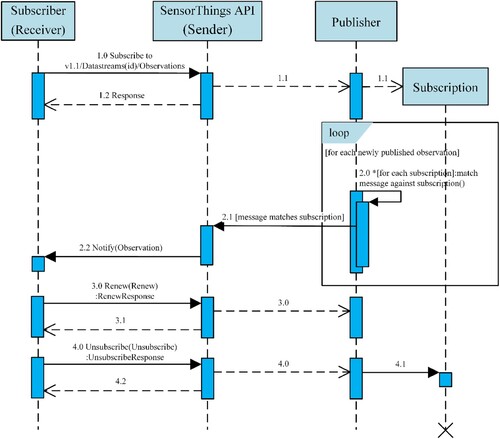
In the context of initiating a Pub/Sub message (data) exchange, the first step involves the creation of a subscription. A subscription defines the available messages that a Publisher can deliver to the Subscriber who expresses an interest. Implementing the Pub/Sub interface in the SensorThings API enables the Publisher to publish data to the Subscriber, who can then subscribe to this data. The Subscriber, on behalf of a Receiver, initiates a subscription through the Subscribe operation within the SensorThings API (1.0). The SensorThings API then conveys subscription requests to the Publisher via the Pub/Sub proxy. If the publisher accepts the subscription request, it begins the subscription creation process (1.1) and returns a response, thereby notifying the requester through the Pub/Sub proxy of the outcome, indicating whether it was successful or if an exception occurred (1.2).

Upon submitting a subscription, a Subscriber can supply filter criteria. Filter expressions are applied to each message, producing a boolean value. Messages that satisfy all filter expressions in a subscription are considered matches. Filter criteria can be based on message content, message metadata, or other message features.

When a Publisher has new messages, it attempts to match them with each active subscription (2.0). If a message meets the filter criteria of a subscription, the Publisher triggers a delivery process to relay the message to the Pub/Sub proxy within the SensorThings API (2.1). Messages are delivered asynchronously as they become accessible to the Publisher. Subsequently, the Pub/Sub proxy notifies the Subscriber (2.2), and the message is further delivered to the Subscriber, effectively concluding the entire publish-subscribe process.

Each subscription has a specified expiration time. Upon reaching this time, the Publisher terminates the subscription. A new expiration time can be set using a Renew operation (3.0). If the Publisher accepts the request, the new expiration time is set on the subscription, and the Publisher returns a response (3.1) to inform the Subscriber of the request outcome.

At any point after creating a subscription, it is possible to use an Unsubscribe operation (4.0) to request the termination of the subscription. If the Publisher accepts the request, it terminates the subscription (4.1) and returns a response (4.2) to inform the Subscriber of the request outcome.

In terms of the data format transmitted in SensorThings API or Pub/Sub, it can either be the serialized representation of the data itself or the Uniform Resource Locator (URL) of the data. For example, raster data can be converted into a byte array for transmission, or the URL of the file in any format (e.g. GeoTIFF, GeoZarr and NetCDF) can be directly transmitted.

3.3. Cloud-based processing of the RTGDC

3.3.1. Data organization

When constructing a RTGDC, it is necessary to simultaneous store metadata and data. Firstly, database tables are created and data is inserted according to the logical model. This involves forming tables for SpatialDimension, SpatialDimensionLevel, TemporalDimension, TemporalDimensionLevel, SensorDimension, ObservationDimension, ObservationMeasure, along with inserting corresponding metadata into these tables.

Secondly, diverse storage strategies are applied to different data types. For raster data, we utilize an object storage strategy and organize them in Cloud Optimized GeoTIFF (COG), a cloud-optimized raster format. Recently, cloud-based object storage services have emerged (Factor et al. 2005; Liu et al. 2018), supporting object processing and byte-range reading, providing new avenues for the rapid retrieval of file content. This allows for cloud optimization of raster-organized files, supporting internal tile retrieval. COG defines the offset (starting byte) and byte count for internal tiles, enabling the swift location and retrieval of tile data in distributed object storage cloud services (Masó 2023). Moreover, by implementing object storage cloud services and adhering to the organizational structure of COG, it not only facilitates multi-level pyramid reading and spatial range-based partial reading but also accommodates large-scale concurrent reads of raster tiles in a cloud environment.

In the RTGDC, unlike the default tile segmentation method starting from the top-left corner in COG, we adopt a different approach by extending the outline pixels of the raster (padding with nodata) before segmentation and then proceeding with the customized tiling scheme. The customized tiling scheme in RTGDC follows the OGC Two Dimensional Tile Matrix Set and Tile Set Metadata Standard (Masó and Jérôme Jacovella-St-Louis 2022). The Standard specifies fixed spatial extent for each tile and fixed resolution for each level, facilitating the creation of aligned global/local tiled grids with multiple levels (also called overviews). In practice, the target spatial extent (global/local) is initially tiled into a customized tile matrix set (e.g. WebMercatorQuad, WorldWGS84Quad and European ETRS89 Lambert azimuthal equal-area Quad) based on spatial parameters such as coordinate reference system (CRS), resolution, and grid size in pixels. Subsequently, raster data is reprojected into the same CRS and is resampled according to the specified resolution. Finally, raster data is organized in the form of COG, where each level and each tile within COG follows the rule of the specified tile matrix set. This ensures strict alignment of each COG tile's spatial extent with the spatial dimension members defined by the RTGDC.

Vector data is stored using a columnar storage strategy. Unlike traditional row-based storage, columnar storage organizes data by columns, storing all data for each column together. Columnar storage can more efficiently compress data, as values in each column are typically similar, and it can enhance query efficiency for column-based queries. Specific implementation can involve columnar storage databases or file formats such as Apache HBase or GeoParquet. The identifiers for vector data serve as row keys in columnar storage. Column families include the geometry property stored in the Well-Known Binary (WKB) format and other properties stored in the JSON format. To ensure the topological consistency of vector data, it is not physically tiled like raster data; instead, it utilizes logical indexing based on the spatial extent of tiles. In other words, if a vector dataset intersects with multiple spatial dimension members (i.e. the spatial extents of the tiles defined in tile matrix set), this vector data will have multiple values indexed to it in the spatial dimension. When querying any of these values in the spatial dimension, the vector can be retrieved. When retrieved, the vector remains intact. It is worth noting that this situation does not apply to points. For lines, linear referencing and dynamic segmentation techniques are employed (Liu, Yu, and Yue 2022) to accurately record segment information for lines in each spatial dimension member. This involves recording the percentage of the line's length represented by intersection points with the observation cell.

3.3.2. Streaming processing

After the construction of the RTGDC, real-time analysis and computation can be performed using the RTGDC, as illustrated in Figure 5. In this process, the RTGDC assumes the role of a publisher. The RTGDC publishes Observation entities via the SensorThings API, thereby generating observation streams. Depending on different real-time tasks, observation streams, created from observation cells, are classified according to specific rules and sent to their corresponding observation topics.

Figure 5. Workflow diagram for RTGDC analysis and computation.

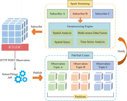
Once observation streams reach the observation topics, the subscriber can pull observation cells from various topics and feed them into the geospatial processing engine. We use Apache Spark Streaming as the geospatial processing engine in RTGDC. The core concept of Spark Streaming is to divide the continuous and real-time observation stream into micro-batches, which are then processed in parallel as Resilient Distributed Datasets (RDDs). This micro-batch processing approach achieves near real-time processing, as each micro-batch is processed within a short time frame, resulting in reduced latency. In this way, Spark Streaming could achieve a reasonable latency while keeping a high throughput. Therefore, in real-time cube computations, Spark Streaming is employed as the computation engine, acting as a subscriber to subscribe to data published by the RTGDC and perform subsequent analysis and computation.

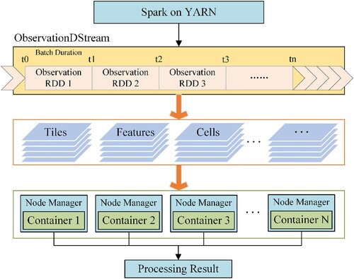
The underlying logic of the Spark Streaming framework, as depicted in Figure 6, is as follows. Upon receiving the observation streams, Spark Streaming transforms them into Spark's in-memory structure, DStream. DStream divides the continuous data stream into small batches, processing each batch as an RDD. In Figure 6, each ObservationRDD undergoes individual RDD operations at the core level. Subsequently, Spark Streaming distributes the data from DStream to containers on various nodes for computation, and then aggregates the computation results from different nodes to obtain the final result. In practice, Spark Streaming is deployed using the YARN (Yet Another Resource Negotiator) mode, which not only harnesses Resource Manager for more efficient task resource allocation and scheduling but also utilizes Node Manager for efficient resource management on each cluster node.

Figure 6. Underlying logic of the Spark Streaming framework.

In the context of real-time cube computation, the Unified Modeling Language (UML) diagram for all computational entities is presented in Figure 7. Observation cells aggregate to form an RTGDC, which includes spatialKey, temporalKey, sensorKey, observationKey, and observationMeasure. ObservationRDD handles the implementation of observation cells while inheriting the abstract RDD structure from Spark. O-CoverageRDD and O-FeatureRDD inherit from ObservationRDD, with their structures being both key-value pairs. In terms of keys, they are identical, containing keys with different dimensions. Their distinction lies in the memory structure of their values (i.e. observation measures). O-CoverageRDD represents measures as RasterTiles, which are tiles of raster data containing spatial information. On the other hand, O-FeatureRDD represents measures as Features, which represent vector data that includes both geometry and properties.

Figure 7. The UML diagram of the RTGDC computation entities.

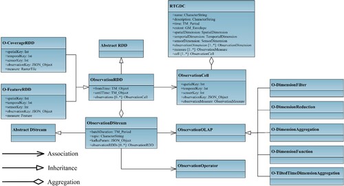
ObservationRDD aggregates over a defined time period to form an ObservationDStream, which acts as the fundamental computational unit in Spark Streaming, inheriting the abstract DStream structure. Prior to generating the ObservationDStream, parameters of the Pub/Sub model are pre-defined, covering topics, batch sizes, and others. ObservationDStream can directly utilize ObservationOperators for computation, which includes a multitude of operators within geospatial processing engines. Additionally, it can undergo computation through ObservationOLAP. ObservationOperators are atomic functions within RTGDC, capable of performing simple operations such as ‘add’, ‘subtract’, as well as meteorological indices and remote sensing indices. On the other hand, ObservationOLAP represents semantic operations applied within RTGDC and serves as an abstraction of certain sets of operations. For ObservationOLAP, it can be utilized to compute many functions or models as long as they meet the definition of ObservationOLAP. The advantage of ObservationOLAP lies in its ability to effortlessly handle complex queries and multidimensional data analysis, obtaining desired results through the combination of queries/calculations across different dimensions.

3.3.3. Observation OLAP

Extending upon SOLAP of GDCs, we introduce Observation OLAP for observation data and articulate it through mathematical formulas. To accommodate spatial entities in vector data, the data cube is introduced into the spatial domain by adding the spatial dimension and measure, thereby advancing OLAP to Spatial OLAP (Han, Stefanovic, and Koperski 1998; Rivest et al. 2005). In this study, concentrating on observation data, we augment OLAP by introducing spatial dimensions/measures and temporal dimensions/measures, and further integrate real-time computing, thereby propelling OLAP to Observation OLAP.

A GDC is defined as follows:

For a GDC with n dimensions, denoted as $({\mathbb{D}}_1,{\mathbb{D}}_2,{\mathbb{D}}_3,\dots ,{\mathbb{D}}_n)$, with fixed dimension hierarchies, each dimension ${\mathbb{D}}_i$ consists of $d_i$ dimension members, where the dimension member set for ${\mathbb{D}}_i$ is defined as ${\mathbb{D}}_i=\{D_i^k|k=1,2,3,\dots ,d_i\}$, $D_i^k$ denotes the $k$-th dimension member of ${\mathbb{D}}_i$. Dimensions of GDC shall contain the spatial dimension ${\mathbb{D}}_{\mathrm{spatial}}$ and the temporal dimension ${\mathbb{D}}_{\mathrm{temporal}}$, since these two dimensions are inherent dimensions that distinguish the GDC from other data cubes.

Any cell within a cube is defined as the binary tuple represented by Eq. (1(1) $\mathrm{Cel}{l}_i=(v,m)$(1) ). (1) $\mathrm{Cel}{l}_i=(v,m)$(1)

where, $v=(v_1,v_2,v_3,\dots ,v_n),v_i\in {\mathbb{D}}_i$. $v$ denotes the dimension vector of $\mathrm{Cel}{l}_i$. $v_i$, which is the $i$-th vector component of $v$, denotes the dimension member used in the $i$-th dimension of $\mathrm{Cel}{l}_i$. $m$ denotes the measure that $\mathrm{Cel}{l}_i$ signifies. Considering that a GDC can handle data from multiple sources, measures can take various forms.

Furthermore, a GDC can be defined as the set represented by Eq. (2(2) $\mathrm{Cube}=\underset{i=1}{\overset{\prod _{i=1}^n{d}_i}{\cup }}\{\mathrm{Cel}{l}_i\}$(2) ). (2) $\mathrm{Cube}=\underset{i=1}{\overset{\prod _{i=1}^n{d}_i}{\cup }}\{\mathrm{Cel}{l}_i\}$(2) where, $\mathrm{Cube}$ denotes the collection of all cells, where the number of cells is determined by multiplying the number of dimension members in each dimension of the cube (i.e. $\prod _{i=1}^n{d}_i$). It is important to note that a cube may be sparse, so the actual number of cells might be much smaller than $\prod _{i=1}^n{d}_i$. In practice, we only make use of those cells that hold data.

Based on the formulas of GDC, Observation OLAP comprises the following components:

1. Dimension Filter: This entails performing Slice queries to select one specific dimension member from a particular dimension, or Dice queries to select a specific set of dimension members from a particular dimension. For $D_{\mathrm{spatial}}$ and $D_{\mathrm{temporal}}$, the semantics can be mapped to spatiotemporal point/range query.

The formula for the Slice query is shown in Eq. (3(3) $\mathrm{Cub}{e}_{\mathrm{Slice}}=\{(v,m)|(v,m)\in \mathrm{Cube}\mathrm{and}{v}_i=D_i^k\}$(3) ), where $i$ denotes the specified dimension for the Slice query,$v_i$ is the $i$-th vector component of $v$, and $D_i^k\in {\mathbb{D}}_i$ denotes the specific dimension member from the $i$-th dimension being queried. (3) $\mathrm{Cub}{e}_{\mathrm{Slice}}=\{(v,m)|(v,m)\in \mathrm{Cube}\mathrm{and}{v}_i=D_i^k\}$(3)

The formula for the Dice query is depicted in Eq. (4(4) $\mathrm{Cub}{e}_{\mathrm{Dice}}=\{(v,m)|(v,m)\in \mathrm{Cube}\mathrm{and}{v}_i\in {\mathbb{D}}_i^{\mathrm{Subset}}\}$(4) ), involving a combined query with two or more dimension members of $i$-th dimension, where ${\mathbb{D}}_i^{\mathrm{Subset}}\subseteq {\mathbb{D}}_i$, are a specific set of dimension members from the $i$-th dimension being queried, and$v_i$ is the $i$-th vector component of $v$. (4) $\mathrm{Cub}{e}_{\mathrm{Dice}}=\{(v,m)|(v,m)\in \mathrm{Cube}\mathrm{and}{v}_i\in {\mathbb{D}}_i^{\mathrm{Subset}}\}$(4)

(2)

Dimension Reduction: Dimension Reduction involves reducing a specific dimension using a particular function, such as summation, averaging, regression, and so on. After this operation, the dimension will disappear. For $D_{\mathrm{spatial}}$ and $D_{\mathrm{temporal}}$, the semantics can be mapped to spatiotemporal merge operation, global spatiotemporal statistical analysis, etc.

The formula for the Dimension Reduction is presented in Eq. (7(7) $\mathrm{Cub}{e}_{\mathrm{Reduce}}=\underset{\begin{array}{c}j=1\end{array}}{\overset{N}{\cup }}\{(g_j,F(i,\mathrm{Group}(g_j)))\}$(7) ), where $i$ denotes the index of the dimension to be reduced, $F$ denotes the function applied to perform the reduction on this dimension, $g_j$ (Eq. (6(6) $g_j=(D_1^{j_1},D_2^{j_2},\dots ,D_{i-1}^{j_{i-1}},D_{i+1}^{j_{i+1}},\dots ,D_n^{j_n}),j=1,2,\dots ,N$(6) )) is an $n-1$-dimensional vector lacking the $i$-th component that is extracted from all dimension members of different dimensions (except $i$-th) in a cube (a total of $N$, i.e. $j=1,2,\dots ,N$), used to gather all cells of a cube with all components the same except the $i$-th one. These cells form a set $\mathrm{Group}(g_j)$ as illustrated in Eq. (5(5) $\mathrm{Group}(g_j)=\{(v,m)|(v,m)\in \mathrm{Cube}\mathrm{and}(v_1,v_2,\dots v_{i-1},v_{i+1},\dots ,v_n)=g_j\}$(5) ). Then, $\mathrm{Cub}{e}_{\mathrm{Reduce}}$ aims to utilize the $F$ function to reduce all cells within the $\mathrm{Group}(g_j)$ into a single cell. The dimension vector of this single cell is $g_j$. (5) $\mathrm{Group}(g_j)=\{(v,m)|(v,m)\in \mathrm{Cube}\mathrm{and}(v_1,v_2,\dots v_{i-1},v_{i+1},\dots ,v_n)=g_j\}$(5) (6) $g_j=(D_1^{j_1},D_2^{j_2},\dots ,D_{i-1}^{j_{i-1}},D_{i+1}^{j_{i+1}},\dots ,D_n^{j_n}),j=1,2,\dots ,N$(6) (7) $\mathrm{Cub}{e}_{\mathrm{Reduce}}=\underset{\begin{array}{c}j=1\end{array}}{\overset{N}{\cup }}\{(g_j,F(i,\mathrm{Group}(g_j)))\}$(7)

(3)

Dimension Aggregation: Dimension Aggregation involves grouping and aggregating dimension members with similar characteristics from a specific dimension using a designated function. For instance, in the context of a speed dimension for trajectory data at a given moment, all speeds can be grouped into categories like $\{v\le 30\mathrm{km}/h\mathrm{or}30\mathrm{km}/h<v\le 60\mathrm{km}/h\mathrm{or}60\mathrm{km}/h⟨v\le 90\mathrm{km}/h\mathrm{or}v⟩90\mathrm{km}/h\}$, and the number of trajectory points in each group can be calculated. For $D_{\mathrm{spatial}}$ and $D_{\mathrm{temporal}}$, the semantics can be mapped to spatiotemporal overlay operation, local spatiotemporal statistical analysis, etc.

The formula for Dimension Aggregation is represented in Eq. (10(10) $\mathrm{Group}(g_j{)}^k=\{(v,m)|(v,m)\in \mathrm{Cube}\mathrm{and}(v_1,v_2,\dots v_{i-1},v_{i+1},\dots ,v_n)=g_j\mathrm{and}{v}_i\in D_i^k\}$(10) ), where $i$ denotes the dimension to be aggregated, $F$ denotes the function applied for aggregation within this dimension. For ${\mathbb{D}}_i$, due to the reorganization of dimension members, a new set of dimension members ${\mathbb{D}}_i^{\mathrm{Aggregate}}$ is obtained (Eq. (8(8) ${\mathbb{D}}_i^{\mathrm{Aggregate}}=\{D_i^k|k=1,2,3,\dots ,d_i^{\mathrm{Aggregate}}\}$(8) )), consisting of $d_i^{\mathrm{Aggregate}}$ members. $g_j$ (Eq. (9(9) $g_j=(D_1^{j_1},D_2^{j_2},\dots ,D_{i-1}^{j_{i-1}},D_{i+1}^{j_{i+1}},\dots ,D_n^{j_n}),j=1,2,\dots ,N$(9) )) is an $n-1$-dimensional vector lacking the $i$-th component that is extracted from all dimension members of different dimensions (except $i$-th) in a cube (a total of $N$, i.e. $j=1,2,\dots ,N$), used to gather all cells of a cube with all components the same except the $i$-th one. $\mathrm{Group}(g_j{)}^k$ denotes a set where the $i$-th vector component belongs to $D_i^k$ and the combination of other vector components equals $g_j$. Then, $\mathrm{Cub}{e}_{\mathrm{Aggregate}}$ aims to utilize the $F$ function to aggregate all cells within the $\mathrm{Group}(g_j{)}^k$ into a single cell. (8) ${\mathbb{D}}_i^{\mathrm{Aggregate}}=\{D_i^k|k=1,2,3,\dots ,d_i^{\mathrm{Aggregate}}\}$(8) (9) $g_j=(D_1^{j_1},D_2^{j_2},\dots ,D_{i-1}^{j_{i-1}},D_{i+1}^{j_{i+1}},\dots ,D_n^{j_n}),j=1,2,\dots ,N$(9) (10) $\mathrm{Group}(g_j{)}^k=\{(v,m)|(v,m)\in \mathrm{Cube}\mathrm{and}(v_1,v_2,\dots v_{i-1},v_{i+1},\dots ,v_n)=g_j\mathrm{and}{v}_i\in D_i^k\}$(10) (11) $\mathrm{Cub}{e}_{\mathrm{Aggregate}}=\underset{j=1}{\overset{N}{\cup }}\underset{k=1}{\overset{d_i^{\mathrm{Aggregate}}}{\cup }}\{((v_1,v_2,\dots v_{i-1},D_i^k,v_{i+1},\dots ,v_n),F(i,\mathrm{Group}{(g_j)}^k))\}$(11)

(4)

Dimension Function: Dimension Function involves the calculation of a specific dimension using a designated function. This may include custom functions on a spectral band dimension, such as the NDVI function: $(\mathrm{NIR}-R)/(\mathrm{NIR}+R)$. Alternatively, it can encompass the computation of functions on combinations of dimensions, like creating a custom deep learning function on both product and spectral band dimensions: processing all spectral bands from Sentinel-1 and Gaofen-2 simultaneously using a deep learning function for change detection. For $D_{\mathrm{spatial}}$ and $D_{\mathrm{temporal}}$, the semantics can be mapped to spatiotemporal functions, models, calculations, etc.

The formula for Dimension Function is represented in (13), where $i$ denotes the dimension to which the function is applied, $F$ denotes the function applied within this dimension. $\mathrm{Select}(C)$ (Eq. (12(12) $\mathrm{Select}(C)=\{(v,m)|C((v,m))=\mathrm{true}\}$(12) )) denotes all cube cells that meet the filtering criteria $C$. $v_i^{\mathrm{\prime }}$ denotes the new dimension member on the $i$-th dimension after applying the dimension function. (12) $\mathrm{Select}(C)=\{(v,m)|C((v,m))=\mathrm{true}\}$(12) (13) $\mathrm{Cub}{e}_{\mathrm{Function}}=\mathrm{Cube}\cup \{(v_1,v_2,\dots ,v_i^{{}^{\mathrm{\prime }}},\dots ,v_n),F(i,\mathrm{Select}(C))\}$(13)

(5)

Tilted Time Dimension Aggregation: Tilted Time Dimension Aggregation involves aggregating data within various time windows on the time dimension with a tilted time window. For instance, in the case of temperature data, measurements taken at minute intervals are stored within a 1-hour window, aggregated to an hourly level within a 1-day window, and further aggregated to a daily level within a 1-month window, and so forth.

3.3.4. Real-time performance evaluation

In the RTGDC, the evaluation of real-time performance is an important aspect, with metrics including latency, throughput, and parallel efficiency. Certain metrics may be satisfied by the elastic feature of the cloud computing environment, such as increased computational resources potentially reducing latency and increasing throughput. However, parallel efficiency may decrease. Hence, this paper evaluates not only the efficiency of the system's real-time performance but also its effectiveness in resource utilization.

The latency in the RTGDC is calculated using Eq. (14(14) $\mathrm{Latency}=\{\begin{array}{l}\mathrm{Tim}{e}_{\mathrm{batchProcess}},\mathrm{if}\mathrm{Tim}{e}_{\mathrm{batchProcess}}\le \mathrm{Tim}{e}_{\mathrm{batchDuration}}\\ +\mathrm{\infty },\mathrm{if}\mathrm{Tim}{e}_{\mathrm{batchProcess}}>\mathrm{Tim}{e}_{\mathrm{batchDuration}}\end{array}$(14) ): (14) $\mathrm{Latency}=\{\begin{array}{l}\mathrm{Tim}{e}_{\mathrm{batchProcess}},\mathrm{if}\mathrm{Tim}{e}_{\mathrm{batchProcess}}\le \mathrm{Tim}{e}_{\mathrm{batchDuration}}\\ +\mathrm{\infty },\mathrm{if}\mathrm{Tim}{e}_{\mathrm{batchProcess}}>\mathrm{Tim}{e}_{\mathrm{batchDuration}}\end{array}$(14) where, $\mathrm{Tim}{e}_{\mathrm{batchDuration}}$ denotes the time interval between two processing batches, and $\mathrm{Tim}{e}_{\mathrm{batchProcess}}$ denotes the average processing time per batch of ObservationRDD. If $\mathrm{Tim}{e}_{\mathrm{batchProcess}}\le \mathrm{Tim}{e}_{\mathrm{batchDuration}}$, it indicates that the system can process the batch data within the specified time interval, resulting in the actual latency being the average time per batch. Otherwise, it indicates that the system cannot release computational resources upon the arrival of the next batch of data, resulting in the inability to process the next batch of data, thus the latency is infinite.

The throughput in the RTGDC is calculated using Eq. (15(15) $\mathrm{Throughput}={\displaystyle \frac{\mathrm{DataVolum}{e}_{\mathrm{input}}}{\mathrm{Tim}{e}_{\mathrm{batchProcess}}},\mathrm{if}\mathrm{Latency}\ne +\mathrm{\infty }}$(15) ): (15) $\mathrm{Throughput}={\displaystyle \frac{\mathrm{DataVolum}{e}_{\mathrm{input}}}{\mathrm{Tim}{e}_{\mathrm{batchProcess}}},\mathrm{if}\mathrm{Latency}\ne +\mathrm{\infty }}$(15) where, $\mathrm{DataVolum}{e}_{\mathrm{input}}$ denotes the total amount of data inputted into the system. Throughput denotes the amount of data the system can process within a unit time.

The parallel efficiency in the RTGDC is calculated using Eq. (16(16) $P=(\mathrm{Tim}{e}_{\mathrm{singleProcess}}/\mathrm{Tim}{e}_{\mathrm{batchProcess}})/\mathrm{Cor}{e}_{\mathrm{used}},\mathrm{if}\mathrm{Latency}\ne +\mathrm{\infty }$(16) ): (16) $P=(\mathrm{Tim}{e}_{\mathrm{singleProcess}}/\mathrm{Tim}{e}_{\mathrm{batchProcess}})/\mathrm{Cor}{e}_{\mathrm{used}},\mathrm{if}\mathrm{Latency}\ne +\mathrm{\infty }$(16) The parallel efficiency is defined as the speedup ($\mathrm{Tim}{e}_{\mathrm{singleProcess}}/\mathrm{Tim}{e}_{\mathrm{batchProcess}}$) divided by the number of cores ($\mathrm{Cor}{e}_{\mathrm{used}}$) utilized by the system. $P$ denotes the effectiveness of the system in utilizing computing resources.

In summary, only when $\mathrm{Tim}{e}_{\mathrm{batchProcess}}\le \mathrm{Tim}{e}_{\mathrm{batchDuration}}$ does the system meet the basic real-time requirement. Under this condition, real-time performance is determined by $\mathrm{Latency}$, $\mathrm{Throughput}$ and $P$. Smaller $\mathrm{Latency}$, larger $\mathrm{Throughput}$, and greater $P$ indicate better real-time performance of the system.

4. Implementation and discussion

4.1. Prototype system

In our implementation, we designed and developed an RTGDC system. All use cases were conducted within our developed prototype system, as depicted in Figure 8, illustrating the overall system architecture. In terms of hardware infrastructure, we utilized High-performance Computing (HPC) servers and High-performance Storage (HPS) servers. The prototype system was deployed on a cluster of five servers, each equipped with CentOS 7 as the operating system, 90 CPU cores, 220GB of memory, and a 100TB storage disk array.

Figure 8. Overall architecture of the RTGDC system.

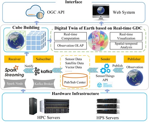
Furthermore, we implemented the OGC Pub/Sub interface Standard and OGC SensorThings API. Once observation data are generated, the system instantaneously publishes them through the SensorThings API. The SensorThings API serves as the hub for managing all data in a Pub/Sub manner, ensuring real-time data subscription for subscribers. Subsequently, Kafka subscribes to the data from the Pub/Sub hub according to demand and delivers them to the Spark Streaming computation engine using its producers. Upon receiving these data, Spark Streaming initiates cube construction, thus RTGDC can support the development of the Digital Twin of Earth in terms of the real-time data ingestion and processing.

Regarding interfaces, we integrated OGC API – Coverages, OGC API – Features, and OGC API – Processes to provide external data access and computational service interfaces. Additionally, we developed a web system for interactive access, enhancing the user experience. In this web system, users can operate real-time data ingestion, where the data forms part of the RTGDC. They can also utilize the real-time processing engine for tasks such as real-time computation, real-time visualization, and spatiotemporal analysis. However, the prototype system did not demonstrate certain complex real-time tasks such as topological operations between vectors or semantic associations between data, although these tasks can be implemented in RTGDC through specific methods.

4.2. Use cases – digital twin of Singapore

Currently, OGC is leading the 2023 Federated Marine Spatial Data Infrastructure (FMSDI) Pilot, with the goal of bridging the gap between land and sea. As a participant, our contribution lies in the development and demonstration of a digital twin for land and marine scenarios in the Singapore region. Key tasks in this program are integrating datasets within the digital twin and analyzing ‘what-if’ scenarios.

We implemented an RTGDC to unify the organization and management of land, marine, and coastal data, thereby implementing the digital twin. Table 2 provides an overview of the data sources utilized in our case. For precipitation, temperature, wind speed, and relative humidity data, we incorporated publicly available station data from the Singapore Meteorological Service website (http://www.weather.gov.sg/) at a temporal resolution of 1 min (with a 60-minute resolution for precipitation data).

Table 2. All data used in the case

Data	Temporal Resolution	Type
Administrative Division	/	Vector
Precipitation	60 min	Station (Point)
Temperature	1min	Station (Point)
Wind Speed	1min	Station (Point)
Relative Humidity	1min	Station (Point)

4.2.1. Real-time ingestion

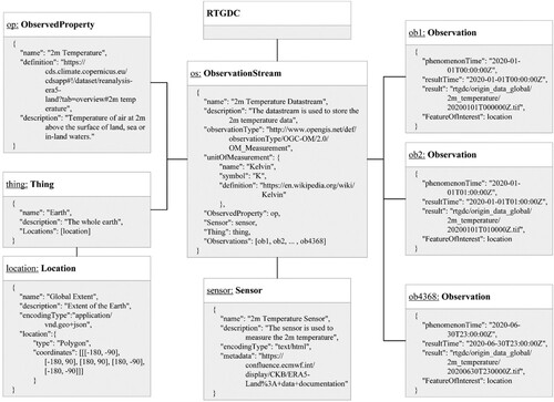
In the study, we published meteorological station data via the SensorThings API, including temperature, relative humidity, precipitation, and wind speed, based on their temporal resolution. According to the definitions of the SensorThings API, a meteorological variable represents an ObservedProperty. Each observation station can be considered a Thing, with its Location being the coordinates of the Thing. The sensors used to monitor these meteorological variables are referred to as Sensors. With these entities in the SensorThings API, ObservationStreams can be created, where each ObservationStream pertains to the same ObservedProperty, utilizing the same Sensor, and generating a stream of Observations within the same Thing. An Observation belongs to a unique ObservationStream, and its FeatureOfInterest can default to the Location of the Thing. Figure 9 serves as an example detecting the temperature ObservationStream within an observation station located at Paya Lebar in Singapore using the temperature sensor, with continuous Observations published in this ObservationStream.

Figure 9. An example modeling for publishing station observations in SensorThings API.

Similar to this example, all other observation stations and meteorological variables were published using the same modeling framework. Observations for these variables were published at intervals of either 1 min or 1 h. Then, taking the temperature variable as an example, the case study shows on how the meteorological data collected from these observation stations is ingested into the RTGDC.

Firstly, when all stations published temperature observations according to the SensorThings API at the timestamp 2023-10-17T20:00:00, Kafka immediately notified Spark Streaming. Spark Streaming subscribed to all temperature observations within the timestamp ‘2023-10-17T20:00:00’ using the following API:

http://example.org/v1.0/Observations?$expand=Datastream/ObservedProperty&$filter=resultTime%20eq%202023-10-17T20:00:00Z%20and%20Datastream/ObservedProperty/name%20eq%27Temperature%27

Then, using the simple kriging function, all observations was interpolated to generate raster data with a resolution of approximately 50 meters. Subsequently, we utilized Spark Streaming to construct cubes. During the construction of the RTGDC, raster data was reorganized into COG format and metadata like dimensions was inputted into the database following the organization method outlined in section 3.3.1.

In this scenario, we evaluated various performance metrics of the RTGDC in the processes from the publication of station data to the tiling of COGs and the ingestion of data (metadata) into the database. This provides a benchmark for real-time performance.

In the case study, real-time data ingestion was conducted only for four variables: temperature, relative humidity, precipitation, and wind speed in the RTGDC. However, to evaluate the scalability of the RTGDC, control experiments were also conducted with 100 and 200 variables. When there are 200 variables, the maximum size of the data that RTGDC holds at one specific time is approximately 900MB. As shown in Figure 10, the analysis results of latency, throughput, and computational efficiency were obtained under different scenarios utilizing various computing resources.

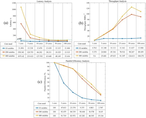
Figure 10. The analysis results of real-time station data ingestion: (a) latency; (b) throughput; (c) parallel efficiency.

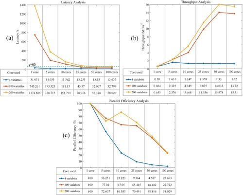
In terms of latency (Figure 10 (a)), since observations are published at 1-minute intervals, each batch of data must be processed within 60 s. When there are only 4 variables, latency meets the requirement for all cases. With 100 variables, the requirement is met when the number of cores reaches 25. With 200 variables, the requirement is met when the number of cores reaches 50. Additionally, overall, a higher number of cores results in shorter processing time (latency) for the data. However, as the number of cores continues to increase, there is a slight decrease in performance due to increased communication time between cores.

Regarding throughput (Figure 10 (b)), under the condition of meeting latency requirements, the maximum throughput for the three scenarios is 1.631, 14.033, and 15.978 MB/s, respectively. It's worth noting that the throughput is strongly correlated with the algorithm used. For the same amount of data, using a simpler algorithm may significantly increase throughput. For example, throughput of RTGDC can be as high as 400MB/s for visualization only. Therefore, here we only represent the throughput of the entire process from station observation publication, interpolation to data ingestion. Overall, throughput also increases with the increase in computing resources.

As for parallel efficiency (Figure 10 (c)), it generally decreases with the increase in computational resources. Therefore, in practical applications, it is not advisable to solely pursue low latency without considering the decrease in resource utilization efficiency brought about by the increase in resources. For example, when processing 100 variables, using 25 cores already achieves low latency and high throughput, with parallel efficiency at a high level. In this case, there is no need to use 50 cores.

4.2.2. Real-time visualization

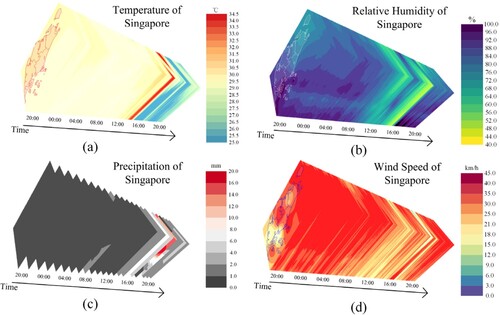
After the real-time data ingestion in RTGDC, the system can visualize meteorological variables such as temperature, relative humidity, precipitation, and wind speed from the RTGDC using the real-time processing approach outlined in section 3.3.2. As depicted in Figure 11, the visualization results span from 20:00 to the following day at 20:00. For 1-minute interval data, a 24-hour dataset consists of 1440 raster files. In the web system, we utilize the CesiumJS, an open source JavaScript library, to visualize the raster and vector data.

Figure 11. Cumulative visualization of real-time meteorological data in Singapore over 24 h: (a) temperature; (b) relative humidity; (c) precipitation; (d) wind speed.

4.2.3. Observation OLAP

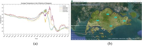
Besides real-time visualizations, this case study encompassed dimension aggregation operation, which is the regional statistical analysis based on Singapore's five administrative divisions: Central Region, Northeast Region, Northwest Region, Southeast Region, and Southwest Region. The primary aim was to validate the OLAP framework in RTGDC. This dimension aggregation operation involved aggregating data across various spatial extents (i.e. the five administrative divisions). Its essence lies in overlaying raster data and vector data, executing intersection operations with raster data based on the five features of vector data. After identifying all intersecting pixels, the operation aggregates them to compute the average value, which serves as the average value of raster data within the respective feature.

Upon the receipt of data by Spark Streaming, the spatial dimension aggregation function was triggered, facilitating real-time calculation of average temperatures for each administrative division. As depicted in Figure 12, the line chart (a) illustrates minute-by-minute temperature variations over the course of a day, while (b) showcases the real-time display interface in the system.

Figure 12. Minute-by-minute temperature changes throughout the day in 5 districts of Singapore: (a) line chart; (b) system visualization.

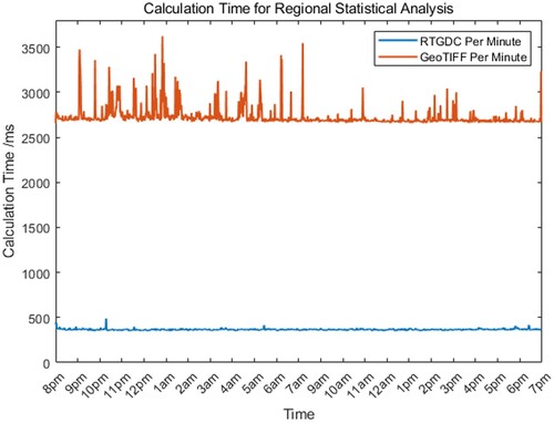
To assess the remarkable performance of the RTGDC in spatiotemporal analysis within the observation OLAP framework, we conducted a comparative time analysis of regional statistics in an identical software and hardware environment, comparing the use of RTGDC with GeoTIFF. As illustrated in Figure 13, the average computation time when employing RTGDC was 366.4 milliseconds, while the average time when using GeoTIFF was 2727.6 milliseconds. Consequently, using the RTGDC for high-performance computing resulted in significant efficiency gains, accompanied by shorter latency, satisfying real-time computational requirements.

Figure 13. The calculation time for regional statistical analysis using RTGDC and GeoTIFF.

4.3. Use cases – global-scale climate analysis

To validate the effectiveness of the RTGDC for a global-scale digital twin of Earth, we conducted a global-scale real-time climate analysis case using our prototype system. Meteorological data was sourced from the Copernicus Climate Change Service (C3S), specifically from the Climate Data Store (CDS). We selected the ERA5-land dataset (Muñoz Sabater 2019) available in the CDS. This dataset employs data assimilation principles, integrating model data with observational results using physical laws to generate optimal estimates.

In our case implementation, we simulated real-time data generation using historical data from January 1, 2020, to June 30, 2020, comprising a total of 4368 images. Although the interval of the EAR5-land dataset is one hour, we actually published the global-scale meteorological data in EAR5-land dataset at one-minute intervals through the SensorThings API and then ingest the data into RTGDC using Spark Streaming. Once the real-time data cube was constructed, we could visualize and processing meteorological data in real-time within the prototype system.

4.3.1. Real-time ingestion

Unlike the station data in the Singapore case, this use case published raster data. Figure 14 demonstrates how 2 m temperature data from the EAR5-land dataset is published using the SensorThings API. Each raster image represents an Observation, with its ‘result’ property represented by a path in the object storage (MinIO). In other words, what is transmitted in Kafka is the URL of the raster image, rather than its byte stream. After the publication, Spark Streaming subscribed to all images within the timestamp ‘2020-01-01T00:00:00’ using the following API: http://example.org/v1.0/Observations?$filter=resultTime%20eq%202020-01-01T00:00:00Z%20

Figure 14. An example modeling for publishing raster data in SensorThings API.

After the subscription, Spark Streaming can receive the URL of the images, and then pull the byte stream of the raster image from MinIO, thereby generating COG and ingesting it into RTGDC along with metadata.

Since in this case raster data was published, we also conducted performance tests on RTGDC when ingesting raster data. To demonstrate the scalability of RTGDC, we evaluated its performance in ingesting 10, 200, and 400 variables simultaneously. When there are 400 variables, the maximum size of the data that RTGDC holds at one specific time is approximately 6000MB. The real-time performance metrics are illustrated in Figure 15. Regarding latency (Figure 15 (a)), generally, as the number of cores increases, the latency tends to decrease; however, a slight performance degradation may occur with excessively high core counts. In terms of throughput (Figure 15 (b)), due to the absence of complex algorithms like kriging interpolation for raster data, the throughput tends to be higher, reaching up to over 120MB/s. Concerning parallel efficiency (Figure 15 (c)), although the speedup ratio increases with the number of cores, the efficiency tends to decrease. Therefore, in this scenario, the practical processing environment may opt for either 25 or 50 cores based on specific requirements.

Figure 15. The analysis results of real-time raster data ingestion: (a) latency; (b) throughput; (c) parallel efficiency.

4.3.2. Observation OLAP

As illustrated in Figure 16 (a), the data cube was visualized in real-time by specifying values for specific dimensions. There were 9 variables within the observation dimension, 4368 values in the temporal dimension, and 1 specific tile (Africa Area) in the spatial dimension.

Figure 16. Temporal evolution of various meteorological variables using the RTGDC: 2 m temperature, surface sensible heat flux, surface pressure, low vegetation leaf area index, total evaporation, surface runoff, surface net solar radiation, high vegetation leaf area index and total precipitation (from left to right, top to bottom): (a) hourly data; (b) monthly data; (c) half yearly data.

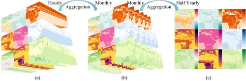
However, due to the uncompressed size of a single image being about 15MB, the total volume of hourly data for 9 variables over a six-month period amounts to 0.56TB, which poses a significant storage burden over time. In many real-time scenarios, outdated data is unnecessary, and only statistical information on outdated data needs to be stored. In this scenario, the Tilted Time Dimension Aggregation in Observation OLAP can be utilized to aggregate the hourly data.

In this setup, we established that once all data for a particular day was published, the hourly data automatically aggregated into daily data; once all data for a month was published, the daily data automatically aggregated into monthly data; and once data for six months was fully published, the monthly data aggregated into a single image.

Figure 16 (b) visualizes the aggregation of hourly data into daily (not shown) and then into monthly data. Figure 16 (c) visualizes the aggregation of monthly data into a single image (average over six months).

By employing Tilted Time Dimension Aggregation, the storage pressure on RTGDC can be significantly alleviated. By configuring different aggregation granularities, only the coarse-grained data required by users can be retained, thus enhancing the availability of RTGDC.

4.3.3. Real-time processing

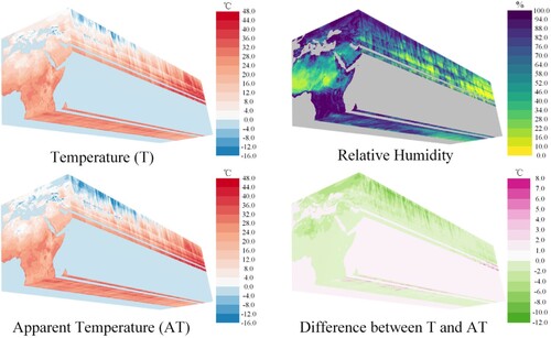
Climate analysis can be conducted within the RTGDC using meteorological models. Notably, the ERA5-land dataset lacks relative humidity data. Nevertheless, we can compute relative humidity using dew point temperature and temperature variables, as outlined in Eq. (18(18) $R=100\ast {\displaystyle \frac{e^{{\displaystyle \frac{a\times \mathrm{TD}}{b+\mathrm{TD}}}}}{e^{{\displaystyle \frac{a\times T}{b+T}}}}}$(18) ) (Lawrence 2005). Since the unit of temperature in ERA5 is Kelvin, it is converted to degrees Celsius first (Eq. (17(17) ${}^{\circ }C=K-273.15$(17) )). (17) ${}^{\circ }C=K-273.15$(17)

(18) $R=100\ast {\displaystyle \frac{e^{{\displaystyle \frac{a\times \mathrm{TD}}{b+\mathrm{TD}}}}}{e^{{\displaystyle \frac{a\times T}{b+T}}}}}$(18) where $R$ = Relative Humidity (%), $\mathrm{TD}$ = Dew Point Temperature (°C), $T$ = Temperature (°C), $a=17.625,b=243.04$

After obtaining relative humidity data, we can calculate the apparent temperature. This, when combined with wind speed data, is used to describe the temperature perceived by the human body, distinct from the actual air temperature. If the temperature at a specific grid point drops to ${10}^{\circ }C$ or lower, wind chill ($T_{\mathrm{wc}}$) is applied as the apparent temperature. For temperatures exceeding $80/3^{\circ }C$, heat index ($\mathrm{HI}$) is used to compute the apparent temperature. In the range of ${10}^{\circ }C$ to $80/3^{\circ }C$, the apparent temperature corresponds to the ambient air temperature ($T$). The formula for the apparent temperature is provided in Eq. (19(19) $\mathrm{AT}=\{\begin{array}{c}\mathrm{HI},T>{\displaystyle \frac{80}{3}{}^{\circ }C}\\ T,{10}^{\circ }C<T\le {\displaystyle \frac{80}{3}{}^{\circ }C}\\ T_{\mathrm{wc}},T\le {10}^{\circ }C\end{array}$(19) ) (Ho et al. 2016) as follows. (19) $\mathrm{AT}=\{\begin{array}{c}\mathrm{HI},T>{\displaystyle \frac{80}{3}{}^{\circ }C}\\ T,{10}^{\circ }C<T\le {\displaystyle \frac{80}{3}{}^{\circ }C}\\ T_{\mathrm{wc}},T\le {10}^{\circ }C\end{array}$(19)

The formulas for $\mathrm{HI}$ and $T_{\mathrm{wc}}$ are presented in Eq. (20(20) $\mathrm{HI}=c_1+c_{2}T+c_{3}R+c_4\mathrm{TR}+c_5{T}^2+c_6{R}^2+c_7{T}^{2}R+c_{8}T{R}^2+c_9{T}^2{R}^2$(20) ) and Eq. (21(21) $T_{\mathrm{wc}}=13.12+0.6215T-9.263V^{0.16}+0.323T{V}^{0.16}$(21) ), respectively. (20) $\mathrm{HI}=c_1+c_{2}T+c_{3}R+c_4\mathrm{TR}+c_5{T}^2+c_6{R}^2+c_7{T}^{2}R+c_{8}T{R}^2+c_9{T}^2{R}^2$(20) where $T$ = Temperature (${}^{\circ }C$), $R$ = Relative Humidity (%), $c_1=-8.78469475556,c_2=1.61139411,c_3=2.33854883889,c_4=-0.14611605,c_5=-0.012308094,c_6=-0.0164248277778,c_7=2.211732\times {10}^{-3},c_8=7.2546\times {10}^{-4},\mathrm{and}{c}_9=-3.582\times {10}^{-6}$. (21) $T_{\mathrm{wc}}=13.12+0.6215T-9.263V^{0.16}+0.323T{V}^{0.16}$(21) where $T$ = Temperature (${}^{\circ }C$), $V$ = Wind Speed (m/s).

The time series plots of calculated relative humidity, apparent temperature, and the difference between apparent temperature and temperature are illustrated in Figure 17.

Figure 17. Temporal evolution of calculated meteorological variables using RTGDC.

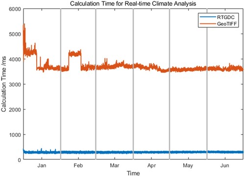
To evaluate the advantages of RTGDC in data organization and the efficient computation using the distributed stream processing engine Spark Streaming, we compared the time taken to compute 4368 images each time using RTGDC and GeoTIFF. As shown in Figure 18, the average time using RTGDC is 277.93 ms, while the average time using GeoTIFF is 3684.49 ms. Therefore, utilizing COG and object storage in RTGDC, along with cloud computing, can significantly enhance its performance.

Figure 18. The calculation time for real-time climate analysis using RTGDC and GeoTIFF.

4.4. Discussion

4.4.1. Achieving the digital twin of earth

The RTGDC, once constructed, may serve as a fundamental component for implementing the Digital Twin of Earth. It is supported by the data delivery model, computation models, as well as high-performance computing.

In terms of data analysis, with high-performance computing clusters or supercomputers, distributed streaming processing frameworks can swiftly handle observational streams from the physical Earth. This process generates real-time analytical results, facilitating the simulation and emulation of the physical Earth. Initially, when real-time observation streams are generated, different types of data can be published to distinct topics using a Pub/Sub model. In the cube construction process, observational streams from different topics are subscribed to. Data are then partitioned according to the specified data splitting rules, and all metadata and data are recorded. Subsequently, within the constructed data cube, various parallel strategies (such as data parallelism and task parallelism) can be applied for parallel computations. This is done using distributed streaming processing frameworks at the level of individual cube cells. High-performance computing clusters are equipped to meet general computational requirements. However, for ultra-high-resolution Digital Twins, supercomputers may be necessary to handle extensive computational demands. Finally, the results of data analysis are visualized, culminating in the simulation and emulation of the physical Earth.

4.4.2. Spatiotemporal analysis of the digital twin of earth

In an RTGDC, using cube cells as the fundamental building blocks and harnessing the strengths of multidimensional data modeling and the robust analytical capabilities of OLAP, it becomes possible to conduct real-time, multiscale spatiotemporal analysis of data within the Digital Twin of Earth. Through spatiotemporal analysis, we can perform real-time visualization, simulation, analysis, computation, and even prediction for data of interest, thereby enhancing the Digital Twin of Earth.

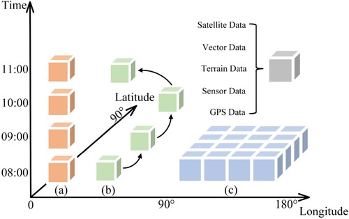
Owing to the RTGDC's capacity to accommodate multiple data sources and organize them along different dimensions, it allows for cell-based real-time spatiotemporal analysis across spatial, temporal, and observation dimensions. Figure 19 depicts spatiotemporal analyses conducted on one or multiple cells corresponding to temporal, observation, and spatial dimensions, respectively. Figure 19 (a) signifies that within the temporal dimension, it is possible to conduct time-series analysis on data from the same spatial dimension and observation dimension, observing its temporal variations over a defined period. Figure 19 (b) highlights that within the observation dimension, it is feasible to trace data from the same observation dimension in both the temporal and spatial dimensions, observing changes across time and space. Figure 19 (c) demonstrates that within the spatial dimension, extensive spatial analysis can be performed on data from the same temporal dimension and observation dimension. In the aforementioned scenarios, a single cell can contain a diverse range of data types, including satellite data, vector data, terrain data, sensor data, GPS data, and more. This allows for real-time multisource data fusion and analysis within the same cell.

Figure 19. Cell-based spatiotemporal analysis for the digital twin of Earth: (a) temporal dimension analysis; (b) observation dimension analysis; (c) spatial dimension analysis.

5. Conclusion

In this paper, we introduce a real-time ingestion and processing approach of geospatial data called the RTGDC, building upon existing GDCs. Our focus is on the realization and enhancement of the DTE in a real-time context.

Firstly, we present an organizational model for the RTGDC, seamlessly integrating the concepts of observations and observation streams into the GDC framework. We design a logical model for RTGDC, providing a solution for the unified organization of vast, heterogeneous, and real-time geospatial data sources. Secondly, we employ a Pub/Sub model in constructing and computing the RTGDC, decoupling the processes of data publishing and subscription. Utilizing the distributed streaming processing framework Spark Streaming, we outline the data Cube's computational workflow, abstracting suitable computational objects for real-time observation data, and introducing OLAP for real-time observation data. Lastly, we applied our methodology to both local-scale (digital twin of Singapore) and global-scale climate analysis to validate our approach. The results demonstrate that RTGDC achieves real-time performance of low latency and high throughput when operating at high levels of parallel efficiency. When processing data using common algorithms, the latency for handling 100MB of data is less than 1 s.

This work offers valuable insights for the further development of RTGDCs and presents a distinctive solution for implementing the DTE. Several avenues for future research include optimizing the efficiency of real-time cube construction and computation for different observation streams, demonstrating the universality of real-time cubes in diverse scenarios, and defining a set of real-time cube APIs to enhance interoperability and external service provision.

Acknowledgment

The work was supported by the National Natural Science Foundation of China (No. 42071354). The work was also supported by Chongqing Technology Innovation and Application Development Project [grant number CSTB2022TIAD-DEX0013], and funding from Chongqing Changan Automobile Co., Ltd, and the Fundamental Research Funds for the Central Universities (2042022dx0001).

Disclosure statement

No potential conflict of interest was reported by the author(s).

Data availability statement

The data and codes that support the findings of this study are available in https://doi.org/ 10.6084/m9.figshare.25688610

 Google Scholar

. Furthermore, the real-time data (see http://www.weather.gov.sg/) of the use case ‘Digital Twin of Singapore' is available online. The ERA5-Land hourly data from 1950 to present (see https://doi.org/ 10.24381/cds.e2161bac

 Google Scholar

) of the use case ‘Global-scale Climate Analysis’ is available online.

Additional information

Funding

The work was supported by the National Natural Science Foundation of China (No. 42071354), and the Natural Science Foundation of Hubei Province (ZRMS2022000666). The work was supported by the Chongqing Technology Innovation and Application Development Project [Grant No. CSTB2022TIAD-DEX0013]; funding from the State Key Laboratory of Intelligent Vehicle Safety Technology and Chongqing Changan Automobile Co. Ltd., and the Fundamental Research Funds for the Central Universities (2042022dx0001).

References

- Abelló, Alberto, Jérôme Darmont, Lorena Etcheverry, Matteo Golfarelli, Jose-Norberto Mazón, Felix Naumann, Torben Pedersen, et al. 2013. “Fusion Cubes: Towards Self-Service Business Intelligence.” International Journal of Data Warehousing and Mining (IJDWM) 9 (2): 66–88. https://doi.org/10.4018/jdwm.2013040104.
- Albergel, C., E. Dutra, J. Muñoz-Sabater, T. Haiden, G. Balsamo, A. Beljaars, L. Isaksen, P. de Rosnay, I. Sandu, and N. Wedi. 2015. “Soil Temperature at ECMWF: An Assessment Using Ground-Based Observations.” Journal of Geophysical Research: Atmospheres 120 (4): 1361–1373. https://doi.org/10.1002/2014JD022505.
- Amani, Meisam, Arsalan Ghorbanian, Seyed A. Ahmadi, Mohammad Kakooei, Armin Moghimi, S. Mohammad Mirmazloumi, Sayyed H. A. Moghaddam, et al. 2020. “Google Earth Engine Cloud Computing Platform for Remote Sensing big Data Applications: A Comprehensive Review.” IEEE Journal of Selected Topics in Applied Earth Observations and Remote Sensing 13: 5326–5350. https://doi.org/10.1109/JSTARS.2020.3021052.
- Annoni, Alessandro, Stefano Nativi, Arzu Çöltekin, Cheryl Desha, Eugene Eremchenko, Caroline M. Gevaert, Gregory Giuliani, et al. 2023. “Digital Earth: Yesterday, Today, and Tomorrow.” International Journal of Digital Earth 16 (1): 1022–1072. https://doi.org/10.1080/17538947.2023.2187467.
- Armstrong, Marc P., Shaowen Wang, and Zhe Zhang. 2019. “The Internet of Things and Fast Data Streams: Prospects for Geospatial Data Science in Emerging Information Ecosystems.” Cartography and Geographic Information Science 46 (1): 39–56. https://doi.org/10.1080/15230406.2018.1503973.
- Bauer, Peter, Bjorn Stevens, and Wilco Hazeleger. 2021. “A Digital Twin of Earth for the Green Transition.” Nature Climate Change 11 (2): 80–83. https://doi.org/10.1038/s41558-021-00986-y.
- Baumann, Peter. 2018. “Datacube Standards and Their Contribution to Analysis-Ready Data.” Proceedings of the International Geoscience and Remote Sensing Symposium, 2051–2053. https://doi.org/10.1109/IGARSS.2018.8518994.
- Baumann, Peter, Andreas Dehmel, Paula Furtado, Roland Ritsch, and Norbert Widmann. 1998. “The Multidimensional Database System RasDaMan”. Proceedings of the 1998 ACM SIGMOD International Conference on Management of Data 27(2): 575–577. https://doi.org/10.1145/276304.276386.
- Baumann, Peter, Andreas Dehmel, Paula Furtado, Roland Ritsch, and Norbert Widmann. 1999. “Spatio-temporal Retrieval with RasDaMan”. Proceedings of the International Conference on Very Large Data Bases 746–749. https://vldb.org/conf/1999/P74.pdf.
- Baumann, Peter, Paolo Mazzetti, Joachim Ungar, Roberto Barbera, Damiano Barbera, Alan Beccati, Lorenzo Bigagli, et al. 2016. “Big Data Analytics for Earth Sciences: The EarthServer Approach.” International Journal of Digital Earth 9 (1): 3–29. https://doi.org/10.1080/17538947.2014.1003106.
- Bergen, Karianne J., Paul A. Johnson, Maarten V. de Hoop, and Gregory C. Beroza. 2019. “Machine Learning for Data-Driven Discovery in Solid Earth Geoscience.” Science 363 (6433): eaau0323. https://doi.org/10.1126/science.aau0323.
- Bhattacharya, D., and M. Painho. 2017. “Smart Cities Intelligence System (Smacisys) Integrating Sensor web with Spatial Data Infrastructures (Sensdi).” ISPRS Annals of the Photogrammetry, Remote Sensing and Spatial Information Sciences IV-4/W3: 21–28. https://doi.org/10.5194/isprs-annals-IV-4-W3-21-2017.
- Bimonte, Sandro, Omar Boucelma, Olivier Machabert, and Sana Sellami. 2014. “A New Spatial OLAP Approach for the Analysis of Volunteered Geographic Information.” Computers, Environment and Urban Systems 48: 111–123. https://doi.org/10.1016/j.compenvurbsys.2014.07.006.
- Braeckel, Aaron, Lorenzo Bigagli, and Johannes Echterhoff. 2016. OGC 13-131r1 OGC Publish/Subscribe Interface Standard 1.0 - Core, Version 1.0. Wayland, MA: Open Geospatial Consortium Inc. http://www.opengis.net/doc/IS/pubsub-core/1.0.
- Carbone, Paris, Asterios Katsifodimos, Stephan Ewen, Volker Markl, Seif Haridi, and Kostas Tzoumas. 2015. “Apache Flink: Stream and Batch Processing in a Single Engine.” The Bulletin of the Technical Committee on Data Engineering 38 (4), http://urn.kb.se/resolve?urn=urn:nbn:se:kth:diva-198940.
- Cardellini, Valeria, Francesco L. Presti, Matteo Nardelli, and Gabriele R. Russo. 2022. “Runtime Adaptation of Data Stream Processing Systems: The State of the art.” ACM Computing Surveys 54 (11s): 1–36. https://doi.org/10.1145/3514496.
- Chen, Nengcheng, Wenying Du, Fan Song, and Zeqiang Chen. 2015. “FLCNDEMF: An Event Metamodel for Flood Process Information Management Under the Sensor web Environment.” Remote Sensing 7 (6): 7231–7256. https://doi.org/10.3390/rs70607231.
- Cody, W. F., J. T. Kreulen, V. Krishna, and W. S. Spangler. 2002. “The Integration of Business Intelligence and Knowledge Management.” IBM Systems Journal 41 (4): 697–713. https://doi.org/10.1147/sj.414.0697.
- Cristescu, Marian P. 2017. “Using OLAP Data Cubes in Business Intelligence.” Scientific Bulletin 21 (2): 80–86. https://doi.org/10.1515/bsaft-2016-0039.
- Cugola, Gianpaolo, and Alessandro Margara. 2012. “Processing Flows of Information: From Data Stream to Complex Event Processing.” ACM Computing Surveys (CSUR), 44(3): 1–62. https://doi.org/10.1145/2187671.2187677.
- DeFelipe, Irene, Juan Alcalde, Eldar Baykiev, Isabel Bernal, Kittiphon Boonma, Ramon Carbonell, Stephanie Flude, et al. 2022. “Towards a Digital Twin of the Earth System: Geo-Soft-CoRe, a Geoscientific Software & Code Repository.” Frontiers in Earth Science 10: 828005. https://doi.org/10.3389/feart.2022.828005.
- Dhu, Trevor, Bex Dunn, Ben Lewis, Leo Lymburner, Norman Mueller, Erin Telfer, Adam Lewis, Alexis McIntyre, Stuart Minchin, and Claire Phillips. 2017. “Digital Earth Australia–Unlocking new Value from Earth Observation Data.” Big Earth Data 1 (1-2): 64–74. https://doi.org/10.1080/20964471.2017.1402490.
- Eugster, Patrick T., Pascal A. Felber, Rachid Guerraoui, and Anne M. Kermarrec. 2003. “The Many Faces of Publish/Subscribe.” ACM Computing Surveys) 35(2): 114–131. https://doi.org/10.1145/857076.857078.
- Factor, Michael, Kalman Meth, Dalit Naor, Ohad Rodeh, and Julian Satran. 2005. “Object Storage: The Future Building Block for Storage Systems.” Proceedings of the International Symposium on Mass Storage Systems and Technology, 119–123. https://doi.org/10.1109/LGDI.2005.1612479.
- Flouris, Ioannis, Nikos Giatrakos, Antonios Deligiannakis, Minos Garofalakis, Michael Kamp, and Michael Mock. 2017. “Issues in Complex Event Processing: Status and Prospects in the big Data era.” Journal of Systems and Software 127: 217–236. https://doi.org/10.1016/j.jss.2016.06.011.
- Fragkoulis, Marios, Paris Carbone, Vasiliki Kalavri, and Asterios Katsifodimos. 2023. “A Survey on the Evolution of Stream Processing Systems.” The VLDB Journal 33 (2): 507–541. https://doi.org/10.1007/s00778-023-00819-8.
- Gao, Fan, Peng Yue, Zhipeng Cao, Shuaifeng Zhao, Boyi Shangguan, Liangcun Jiang, Lei Hu, Zhe Fang, and Zheheng Liang. 2022. “A Multi-Source Spatio-Temporal Data Cube for Large-Scale Geospatial Analysis.” International Journal of Geographical Information Science 36 (9): 1853–1884. https://doi.org/10.1080/13658816.2022.2087222.
- Gettelman, Andrew, Alan J. Geer, Richard M. Forbes, Greg R. Carmichael, Graham Feingold, Derek J. Posselt, Graeme L. Stephens, Susan C. Van den Heever, Adam C. Varble, and Paquita Zuidema. 2022. “The future of Earth system prediction: Advances in model-data fusion.” Science Advances 8(14): eabn3488. https://doi.org/10.1126/sciadv.abn3488.
- Gong, Jianya, Longgang Xiang, Jin Chen, Peng Yue, and Yi Liu. 2011. ““GeoGlobe: A Virtual Globe for Multi-Source Geospatial Information Integration and Service.” Advances in Web-Based GIS, Mapping Services and Applications 9: 85. https://doi.org/10.1201/b11080-9.
- Goodchild, Michael F. 2008. “The use Cases of Digital Earth.” International Journal of Digital Earth 1 (1): 31–42. https://doi.org/10.1080/17538940701782528.
- Goodchild, Michael F. 2013. “The Quality of big (geo) Data.” Dialogues in Human Geography 3 (3): 280–284. https://doi.org/10.1177/2043820613513392.
- Goodchild, Michael F., Huadong Guo, Alessandro Annoni, Ling Bian, Kees de Bie, Frederick Campbell, Max Craglia, et al. 2012. “Next-generation Digital Earth.” Proceedings of the National Academy of Sciences 109 (28): 11088–11094. https://doi.org/10.1073/pnas.1202383109.
- Gorelick, Noel, Matt Hancher, Mike Dixon, Simon Ilyushchenko, David Thau, and Rebecca Moore. 2017. “Google Earth Engine: Planetary-Scale Geospatial Analysis for Everyone.” Remote Sensing of Environment 202: 18–27. https://doi.org/10.1016/j.rse.2017.06.031.
- Grossner, Karl E., Michael F. Goodchild, and Keith C. Clarke. 2008. “Defining a Digital Earth System.” Transactions in GIS 12 (1): 145–160. https://doi.org/10.1111/j.1467-9671.2008.01090.x.
- Guo, Huadong, Xiangtao Fan, and Changlin Wang. 2009. “A Digital Earth Prototype System: DEPS/CAS.” International Journal of Digital Earth 2 (1): 3–15. https://doi.org/10.1080/17538940902746512.
- Guo, Huadong, Michael F. Goodchild, and Alessandro Annoni. 2020. Manual of digital earth. London: Springer Nature. https://doi.org/10.1007/978-981-32-9915-3.
- Guo, Huadong, Zhen Liu, Hao Jiang, Changlin Wang, Jie Liu, and Dong Liang. 2017. “Big Earth Data: A new Challenge and Opportunity for Digital Earth’s Development.” International Journal of Digital Earth 10 (1): 1–12. https://doi.org/10.1080/17538947.2016.1264490.
- Hamdani, Younes, Guohui Xiao, Linfang Ding, and Diego Calvanese. 2023. “An Ontology-Based Framework for Geospatial Integration and Querying of Raster Data Cube Using Virtual Knowledge Graphs.” ISPRS International Journal of Geo-Information 12 (9): 375. https://doi.org/10.3390/ijgi12090375.
- Han, Jiawei, Nebojsa Stefanovic, and Krzysztof Koperski. 1998. “Selective Materialization: An Efficient Method for Spatial Data Cube Construction.” Proceedings of the Second Pacific-Asia Conference on Research and Development in Knowledge Discovery and Data Mining, 1394: 144–158. https://doi.org/10.1007/3-540-64383-4_13.
- Ho, Hung C., Anders Knudby, Yongming Xu, Matus Hodul, and Mehdi Aminipouri. 2016. “A Comparison of Urban Heat Islands Mapped Using Skin Temperature, air Temperature, and Apparent Temperature (Humidex), for the Greater Vancouver Area.” Science of the Total Environment 544: 929–938. https://doi.org/10.1016/j.scitotenv.2015.12.021.
- Hoffmann, Jörn, Peter Bauer, Irina Sandu, Nils Wedi, Thomas Geenen, and Daniel Thiemert. 2023. “Destination Earth–A Digital Twin in Support of Climate Services.” Climate Services 30: 100394. https://doi.org/10.1016/j.cliser.2023.100394.
- Huang, Thomas, Cedric David, Catalina Oadia, Joe T. Roberts, Sujay V. Kumar, Paul Stackhouse, David Borges, Simon Baillarin, Gwendoline Blanchet, and Peter Kettig. 2022. “An Earth System Digital Twin for Flood Prediction and Analysis.” Proceedings of the International Geoscience and Remote Sensing Symposium, 4735–4738. https://doi.org/10.1109/IGARSS46834.2022.9884830.
- Iqbal, Muhammad H., and Tariq R. Soomro. 2015. “Big Data Analysis: Apache Storm Perspective.” International Journal of Computer Trends and Technology 19 (1): 9–14. https://doi.org/10.14445/22312803/IJCTT-V19P103.
- Isah, Haruna, Tariq Abughofa, Sazia Mahfuz, Dharmitha Ajerla, Farhana Zulkernine, and Shahzad Khan. 2019. “A Survey of Distributed Data Stream Processing Frameworks.” IEEE Access 7: 154300–154316. https://doi.org/10.1109/ACCESS.2019.2946884.
- ISO/TC 211. 2023. “ISO 19156:2023, Geographic Information — Observations, Measurements and Samples.” https://www.iso.org/standard/82463.html.
- Jacovella-St-Louis, Jérôme. 2022. OGC Testbed 17: Geo Data Cube API Engineering Report. Wayland, MA: Open Geospatial Consortium. http://www.opengis.net/doc/PER/t17-D012.
- Khazael, Behnam, Mojtaba V. Asl, and Hadi T. Malazi. 2023. “Geospatial Complex Event Processing in Smart City Applications.” Simulation Modelling Practice and Theory 122: 102675. https://doi.org/10.1016/j.simpat.2022.102675.
- Kienberger, Stefan, and Dirk Tiede. 2008. “ArcGIS Explorer Review.” GEO Informatics 11 (2): 42–47. https://www.academia.edu/download/71835975/ArcGIS_Explorer_Review_Is_This_Yet_Anoth20211007-9678-1uy4zb.pdf.
- Killough, Brian. 2018. “Overview of the Open Data Cube Initiative.” Proceedings of the International Geoscience and Remote Sensing Symposium, 8629–8632. https://doi.org/10.1109/IGARSS.2018.8517694.
- Kiran, Mariam, Peter Murphy, Inder Monga, Jon Dugan, and Sartaj S. Baveja. 2015. “Lambda Architecture for Cost-Effective Batch and Speed Big Data Processing.” Proceedings of the International Conference on Big Data (Big Data) 2785-2792. https://doi.org/10.1109/BigData.2015.7364082.
- Kulkarni, Sanjeev, Nikunj Bhagat, Maosong Fu, Vikas Kedigehalli, Christopher Kellogg, Sailesh Mittal, Jignesh M. Patel, Karthikeyan Ramasamy, and Siddarth Taneja. 2015. “Twitter Heron: Stream Processing at Scale.” Proceedings of the ACM SIGMOD International Conference on Management of Data, 239–250. https://doi.org/10.1145/2723372.2742788.
- Lawrence, Mark G. 2005. “The Relationship Between Relative Humidity and the Dewpoint Temperature in Moist air: A Simple Conversion and Applications.” Bulletin of the American Meteorological Society 86 (2): 225–234. https://doi.org/10.1175/BAMS-86-2-225.
- Lazidis, Apostolos, Konstantinos Tsakos, and Euripides G. M. Petrakis. 2022. “Publish–Subscribe Approaches for the IoT and the Cloud: Functional and Performance Evaluation of Open-Source Systems.” Internet of Things 19: 100538. https://doi.org/10.1016/j.iot.2022.100538.
- Lewis, Adam, Leo Lymburner, Matthew B. J. Purss, Brendan Brooke, Ben Evans, Alex Ip, et al. 2016. “Rapid, High-Resolution Detection of Environmental Change Over Continental Scales from Satellite Data–the Earth Observation Data Cube.” International Journal of Digital Earth 9 (1): 106–111. https://doi.org/10.1080/17538947.2015.1111952.
- Lewis, Adam, Simon Oliver, Leo Lymburner, Ben Evans, Lesley Wyborn, Norman Mueller, Gregory Raevksi, et al. 2017. “The Australian Geoscience Data Cube—Foundations and Lessons Learned.” Remote Sensing of Environment 202: 276–292. https://doi.org/10.1016/j.rse.2017.03.015.
- Li, Songnian, Suzana Dragicevic, Francesc A. Castro, Monika Sester, Stephan Winter, Arzu Coltekin, Christopher Pettit, et al. 2016. “Geospatial big Data Handling Theory and Methods: A Review and Research Challenges.” ISPRS Journal of Photogrammetry and Remote Sensing 115: 119–133. https://doi.org/10.1016/j.isprsjprs.2015.10.012.
- Li, Xin, Min Feng, Youhua Ran, Yang Su, Feng Liu, Chunlin Huang, Huanfeng Shen, et al. 2023. “Big Data in Earth System Science and Progress Towards a Digital Twin.” Nature Reviews Earth & Environment 4 (5): 319–332. https://doi.org/10.1038/s43017-023-00409-w.
- Li, Haifeng, and Xinsha Fu. 2011. “An Intelligence Traffic Accidence Monitor System Using Sensor Web Enablement.” Procedia Engineering 15: 2098–2102. https://doi.org/10.1016/j.proeng.2011.08.808.
- Li, Wenwen, Yan Liu, and Sizhe Wang. 2022. Real-time GIS Programming and Geocomputation. Oak Ridge, Tennessee, USA: Oak Ridge National Laboratory. https://doi.org/10.22224/gistbok/2022.1.3.
- Li, Jiyuan, Lingkui Meng, Frank Z. Wang, Wen Zhang, and Yang Cai. 2014. “A map-Reduce-Enabled SOLAP Cube for Large-Scale Remotely Sensed Data Aggregation.” Computers & Geosciences 70: 110–119. https://doi.org/10.1016/j.cageo.2014.05.008.
- Liang, Steve, Tania Khalafbeigi, and Hylke van der Schaaf. 2021. OGC 18-088 OGC SensorThings API Part 1: Sensing Version 1.1, Version 1.1. Wayland, MA: Open Geospatial Consortium Inc. http://www.opengis.net/doc/is/sensorthings/1.1.
- Liu, Jialin, Quincey Koziol, Gregory F. Butler, Neil Fortner, Mohamad Chaarawi, Houjun Tang, Suren Byna, et al. 2018. “Evaluation of HPC Application I/O on Object Storage Systems.” Proceedings of the International Workshop on Parallel Data Storage & Data Intensive Scalable Computing Systems (PDSW-DISCS) 24-34. https://doi.org/10.1109/PDSW-DISCS.2018.00005.
- Liu, Ruixiang, Dayu Yu, and Peng Yue. 2022. “A Disaster Information Service for Damaged Road Networks Using Dynamic Segmentation.” Proceedings of the International Conference on Agro-Geoinformatics (Agro-Geoinformatics) 1-6. https://doi.org/10.1109/Agro-Geoinformatics55649.2022.9859082.
- Livaja, Ivan, Krešimir Pripužić, Siniša Sovilj, and Martin Vuković. 2022. “A Distributed Geospatial Publish/Subscribe System on Apache Spark.” Future Generation Computer Systems 132: 282–298. https://doi.org/10.1016/j.future.2022.02.013.
- Mahdavi-Amiri, Ali, Troy Alderson, and Faramarz Samavati. 2015. “A Survey of Digital Earth.” Computers & Graphics 53: 95–117. https://doi.org/10.1016/j.cag.2015.08.005.
- Mahecha, Miguel D., Fabian Gans, Gunnar Brandt, Rune Christiansen, Sarah E. Cornell, Normann Fomferra, Guido Kraemer, et al. 2020. “Earth System Data Cubes Unravel Global Multivariate Dynamics.” Earth System Dynamics 11 (1): 201–234. https://doi.org/10.5194/esd-11-201-2020.
- Masmoudi, Maroua, Sana B. A. B. Lamine, Zghal Hajer B, Bernard Archimede, and Mohamed H. Karra. 2021. “Knowledge Hypergraph-Based Approach for Data Integration and Querying: Application to Earth Observation.” Future Generation Computer Systems 115: 720–740. https://doi.org/10.1016/j.future.2020.09.029.
- Masó, Joan. 2023. OGC 21-026 OGC Cloud Optimized GeoTIFF Standard, Version 1.0. Wayland, MA: Open Geospatial Consortium Inc. http://www.opengis.net/doc/is/COG/1.0.
- Masó, Joan, and J. Jérôme Jacovella-St-Louis. 2022. OGC 17-083r4 OGC Two Dimensional Tile Matrix Set and Tile Set Metadata, Version 2.0. Wayland, MA: Open Geospatial Consortium Inc. http://www.opengis.net/doc/IS/tms/2.0.
- Mišev, Dimitar, Peter Baumann, Dimitris Bellos, and Stefan Wiehle. 2019. “BigDataCube: A Scalable, Federated Service Platform for Copernicus.” Proceedings of the International Conference on Big Data (Big Data), 4103–4112. https://doi.org/10.1109/BigData47090.2019.9006222.
- Mohammadi, Mehdi, Ala Al-Fuqaha, Sameh Sorour, and Mohsen Guizani. 2018. “Deep Learning for IoT big Data and Streaming Analytics: A Survey.” IEEE Communications Surveys & Tutorials 20 (4): 2923–2960. https://doi.org/10.1109/COMST.2018.2844341.
- Muñoz Sabater, J. 2019. “ERA5-Land Hourly Data from 1950 to Present. Copernicus Climate Change Service (C3S) Climate Data Store (CDS).” Accessed September 11, 2023. https://doi.org/10.24381/cds.e2161bac.
- Oza, Nikunj, Jacqueline LeMoigne, Marge Cole, Morris Robert, Rogers Laura, Seablom Michael, and Smith Benjamin. 2021. “NASA Earth Science Technology for Earth System Digital Twins (ESDT).” In AGU Fall Meeting 2021, New Orleans, LA, USA, SY14A-04, 1–8. https://doi.org/10.1002/essoar.10509965.1.
- Percivall, George. 2020. OGC 18-095r7 Geospatial Coverages Data Cube Community Practice, Version 1.0. Wayland, MA: Open Geospatial Consortium. http://www.opengis.net/doc/CS/dataCubeCP.
- Pires, Ivan M., Nuno M. Garcia, Nuno Pombo, and Francisco Flórez-Revuelta. 2016. “From Data Acquisition to Data Fusion: A Comprehensive Review and a Roadmap for the Identification of Activities of Daily Living Using Mobile Devices.” Sensors 16 (2): 184. https://doi.org/10.3390/s16020184.
- Purss, Matthew B. J., and Jérôme Jacovella-St-Louis. 2021. OGC 21-038 OGC API - Discrete Global Grid Systems - Part 1: Core, Version 1.0. Wayland, MA: Open Geospatial Consortium Inc. https://opengeospatial.github.io/ogcna-auto-review/21-038.html.
- Rajarathinam, Ragul, A. Bhuvaneswari, and R. Jothi. 2022. “A Real-Time Crisis Informatics System by Fusing Geo-Spatial Twitter Streams and User-Posted Images.” Materials Today: Proceedings 62: 4738–4744. https://doi.org/10.1016/j.matpr.2022.03.252.
- Rathore, Muhammad M. U., Anand Paul, Awais Ahmad, Bo-Wei Chen, Bormin Huang, and Wen Ji. 2015. “Real-time big Data Analytical Architecture for Remote Sensing Application.” IEEE Journal of Selected Topics in Applied Earth Observations and Remote Sensing 8 (10): 4610–4621. https://doi.org/10.1109/JSTARS.2015.2424683.
- Rivest, Sonia, Yvan Bédard, Marie J. Proulx, and Martin Nadeau. 2003. “SOLAP: A new Type of User Interface to Support Spatio-Temporal Multidimensional Data Exploration and Analysis.” Proceedings of the ISPRS Joint Workshop on Spatial, Temporal and Multi-Dimensional Data Modelling and Analysis 2-3. https://api.semanticscholar.org/CorpusID:15581781.
- Rivest, Sonia, Yvan Bédard, Marie J. Proulx, Martin Nadeau, Frederic Hubert, and Julien Pastor. 2005. “SOLAP Technology: Merging Business Intelligence with Geospatial Technology for Interactive Spatio-Temporal Exploration and Analysis of Data.” ISPRS Journal of Photogrammetry and Remote Sensing 60 (1): 17–33. https://doi.org/10.1016/j.isprsjprs.2005.10.002.
- Salloum, Salman, Ruslan Dautov, Xiaojun Chen, Patrick X. Peng, and Joshua Z. Huang. 2016. “Big Data Analytics on Apache Spark.” International Journal of Data Science and Analytics 1 (3-4): 145–164. https://doi.org/10.1007/s41060-016-0027-9.
- Schleidt, Katharina, and Stefan Jetschny. 2023a. “FAIRiCUBE: Enabling Gridded Data Analysis for All.” EGU General Assembly 2023, Vienna, Austria, 24–28 Apr 2023, EGU23-7052. https://doi.org/10.5194/egusphere-egu23-7052.
- Schleidt, Katharina, and Ilkka Rinne. 2023b. OGC 20-082r4 OGC Abstract Specification Topic 20: Observations, measurements and samples, Version 3.0.0. Wayland, MA: Open Geospatial Consortium Inc. http://www.opengis.net/doc/as/om/3.0.
- Schramm, Matthias, Edzer Pebesma, Milutin Milenković, Luca Foresta, Jeroen Dries, Alexander Jacob, Wolfgang Wagner, et al. 2021. “The Openeo api–Harmonising the use of Earth Observation Cloud Services Using Virtual Data Cube Functionalities.” Remote Sensing 13 (6): 1125. https://doi.org/10.3390/rs13061125.
- Silva, Dennis S., and Maristela Holanda. 2022. “Applications of Geospatial Big Data in the Internet of Things.” Transactions in GIS 26 (1): 41–71. https://doi.org/10.1111/tgis.12846.
- Soumaya, Ounacer, Talhaoui M. Amine, Ardchir Soufiane, Daif Abderrahmane, and Azouazi Mohamed. 2017. “Real-time Data Stream Processing Challenges and Perspectives.” International Journal of Computer Science Issues (IJCSI) 14 (5): 6–12. https://doi.org/10.20943/01201705.612.
- Sudmanns, Martin, Hannah Augustin, Brian Killough, Gregory Giuliani, Dirk Tiede, Alex Leith, Fang Yuan, and Adam Lewis. 2023. “Think Global, Cube Local: An Earth Observation Data Cube’s Contribution to the Digital Earth Vision.” Big Earth Data 7 (3): 831–859. https://doi.org/10.1080/20964471.2022.2099236.
- Sun, Ziheng, Liping Di, Hui Fang, Chen Zhang, Eugene Yu, Li Lin, Xicheng Tan, and Peng Yue. 2016. “Embedding Pub/Sub Mechanism Into OGC web Services to Augment Agricultural Crop Monitoring.” Proceedings of the International Conference on Agro-Geoinformatics (Agro-Geoinformatics), 1–4. https://doi.org/10.1109/Agro-Geoinformatics.2016.7577653.
- Tamiminia, Haifa, Bahram Salehi, Masoud Mahdianpari, Lindi Quackenbush, Sarina Adeli, and Brian Brisco. 2020. “Google Earth Engine for Geo-Big Data Applications: A Meta-Analysis and Systematic Review.” ISPRS Journal of Photogrammetry and Remote Sensing 164: 152–170. https://doi.org/10.1016/j.isprsjprs.2020.04.001.
- Tu, Doan Q., A. S. M. Kayes, Wenny Rahayu, and Kinh Nguyen. 2020. “IoT Streaming Data Integration from Multiple Sources.” Computing 102 (10): 2299–2329. https://doi.org/10.1007/s00607-020-00830-9.
- Voosen, Paul. 2020. “Europe Builds ‘Digital Twin’ of Earth to Hone Climate Forecasts.” Science 370 (6512): 16–17. https://doi.org/10.1126/science.370.6512.16.
- Wang, Chengshan, Robert M. Hazen, Qiuming Cheng, Michael H. Stephenson, Chenghu Zhou, Peter Fox, Shu-zhong Shen, et al. 2021. “The Deep-Time Digital Earth Program: Data-Driven Discovery in Geosciences.” National Science Review 8 (9): nwab027. https://doi.org/10.1093/nsr/nwab027.
- Wilkinson, Mark D., Michel Dumontier, IJsbrand J. Aalbersberg, Gabrielle Appleton, Myles Axton, Arie Baak, Niklas Blomberg, et al. 2016. “The FAIR Guiding Principles for Scientific Data Management and Stewardship.” Scientific Data 3 (1): 1–9. https://doi.org/10.1038/sdata.2016.18.
- Zhai, Xi, Peng Yue, and Mingda Zhang. 2016. “A Sensor Web and Web Service-Based Approach for Active Hydrological Disaster Monitoring.” ISPRS International Journal of Geo-Information 5 (10): 171. https://doi.org/10.3390/ijgi5100171.
- Zhang, Lei, Hanqing Shi, Zhenzhan Wang, Hong Yu, Xiaobin Yin, and Qixiang Liao. 2018. “Comparison of Wind Speeds from Spaceborne Microwave Radiometers with in Situ Observations and ECMWF Data Over the Global Ocean.” Remote Sensing 10 (3): 425. https://doi.org/10.3390/rs10030425.