A spatial downscaling method for SMAP soil moisture considering vegetation memory and spatiotemporal fusion

ABSTRACT

Soil moisture (SM) plays an essential role in the hydrological cycle, drought monitoring, and water resources management. However, passive microwave remote sensing products offer coarse spatial resolutions (approximately 25–40 km), greatly limiting their applications. In this study, we considered vegetation memory and increased the amount of vegetation data by spatiotemporal fusion, integrated lagged vegetation index and fusion data as model inputs, and downscaled the spatial resolution of SMAP SM using the Random Forest (RF) model as well as multi-source remote sensing data. The downscaled SM was validated with 30 in situ SM measurements and daily precipitation data and explored the contributions of NDVI_lagged and NDVI_fused in downscaling. The results show that the downscaled SM is highly consistent with the in situ SM measurements. The correlation ranges from 0.628 to 0.849 with an average of 0.689. The root mean square error (RMSE) ranges from 0.024 to 0.094 m³/m³ with an average of 0.057 m³/m³. The proposed method leverages the strengths of the RF model, fusion vegetation data, and lagged vegetation data to improve high-resolution SM accuracy.

KEYWORDS:

• Soil moisture downscaling
• SMAP
• random forest
• vegetation memory
• spatiotemporal fusion

1. Introduction

Soil moisture (SM) is a vital variable for hydrological models (Zhuo and Han 2016), ecological models (Liu et al. 2020), climate models (Mimeau et al. 2021), and Land Surface Models (Fisher and Koven 2020), and plays an important role in drought monitoring (Wu and Li 2021), floods forecasting (Meng, Xie, and Liang 2017), heatwaves prediction (Zhang, Jia, and Qian 2022a) and agricultural management (Wang et al. 2021). Hence, it is critical to accurately and detailed obtain the spatial and temporal distribution of surface SM.

In general, there are different ways to monitor SM. The traditional site monitoring methods include the gravimetric method (Schmugge, Jackson, and McKim 1980), neutron probe technology (Chanasyk and Naeth 1996), time domain reflectometry (Yu and Drnevich 2004), and frequency domain reflectometry (Robock et al. 2000), which can provide high precision and temporal resolution SM observation. However, these methods are limited in spatial coverage, as they provide point measurements (Qin et al. 2013).

Satellite remote sensing offers a more convenient and continuous method for observing SM over large areas at various spatial scales. Microwave remote sensing, in particular, can penetrate vegetation canopies, minimizing weather interference. Simultaneously, the backscattering coefficients measured by the microwave sensor can describe the relationship between the soil dielectric constant and water content (Ebrahimi-Khusfi et al. 2018). At present, a number of satellites with microwave sensors have been launched to obtain SM, including Advanced Microwave Scanning Radiometer for the Earth Observing System (AMSR-E) (Mladenova et al. 2014), Advance Microwave Scanning Radiometer-2 (AMSR2), (Zhang et al. 2021) Advanced Scatterometer (ASCAT) (Lindell and Long 2016), Soil Moisture and Ocean Salinity (SMOS) (Wigneron et al. 2021), and Soil Moisture Active Passive (SMAP) (Bhuiyan et al. 2018).

The coarse spatial resolution (25–40 km) of microwave SM products significantly limits their application in hydrology and agriculture. Various approaches have been developed to downscale coarse-resolution SM, including triangle/trapezoid methods (Bai et al. 2019; Zhao and Li 2015), Disaggregation based on Physical And Theoretical scale Change (DISPATCH) (Djamai et al. 2016; Merlin et al. 2013), data assimilation (Lievens et al. 2015; Sahoo et al. 2013), and RF models (Long et al. 2019; Mao et al. 2022). These methods explore the relationship between remotely sensed SM and auxiliary data to generate SM at finer spatial scales (Peng et al. 2017). While high-resolution soil moisture products like the Copernicus 1-km surface soil moisture product, the Theia 100-m soil moisture product, and the recent RT1-based TU Wien 1-km soil moisture product exist, their public availability is currently limited to specific regions in Europe (Brocca, Zhao, and Lu 2023).

Previous downscaling methods often utilize high-resolution auxiliary variables like vegetation index (VI), surface albedo, land surface temperature (LST), and topography. However, few studies have incorporated lagged VI, despite its significance in spatial downscaling and a significant relationship between soil moisture and NDVI (Engstrom et al. 2008; West et al. 2018). On the one hand, soil moisture limits plant transpiration and photosynthesis, ultimately affecting vegetation type and structure (Engstrom et al. 2008). On the other hand, vegetation regulates the SM spatial distribution through the storage, conservation, absorption and consumption of water (Wang and Shi 2019). Additionally, variations in biological processes and plant species lead to spatial discrepancies in SM at different depths and with varying hydraulic properties (Chang et al. 2018; Coenders-Gerrits et al. 2014). Chen et al. (2014) and Zhang, Ji, and Wylie (2011) further confirmed a strong positive correlation between SM and NDVI, with NDVI typically lagging behind SM by 1 month. Meanwhile, remotely sensed NDVI is often incomplete in space and time due to satellite swath width, revisit time, and cloud contamination (Zhu et al. 2010). Consequently, existing downscaling methods are limited to clear-sky conditions, hindering SM application in drought monitoring and water resource management. Fortunately, various data fusion models address these data gaps caused by cloud cover and orbital swaths.

In this study, we intend to downscale SMAP SM by constructing nonlinear relationships between SM and multi-source remote sensing data using spatiotemporal fusion and RF models. We focused on the following objectives: (1) downscale SMAP SM to 1 km × 1 km by integrating NDVI_lagged, NDVI_fused, and other auxiliary data into RF models; (2) validate the accuracy of the downscaled SM estimates using 30 in situ measurements; (3) explore contributions of NDVI_lagged and NDVI_fused to the downscaled SM generated by the proposed approach. The high-resolution SM produced by this method will be valuable for regional hydrological research and water resources management.

2. Study area and materials

2.1. Study area

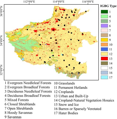
Henan Province (31.38°−36.37°N, 110.35°−116.64°E, Figure 1) is located in Central China and has a warm temperate monsoon climate. The mean annual temperature of 15.6°C, and annual rainfall averages 834.5 mm. It has an obvious seasonal climate with hot and humid summers and cold and dry winters, which favor the growth of various crops (Chen, Zhang, and Tao 2018). The province has varied topography and complex hydrothermal conditions. There is an obvious temperature gradient between the western mountainous and the eastern plains, with higher temperatures in the southeast and lower in the northwest. Due to the uneven spatial and temporal rainfall distribution, Henan Province has suffered frequent droughts (Shi et al. 2017).

Figure 1. Map of land cover classifications in Henan province and distribution of 30 in situ stations. SM observation sites are marked with black dotted symbols. The bottom map is obtained based on MCD12Q1.

2.2. Data description

2.2.1. Soil moisture products

2.2.1.1. SMAP data

The SMAP satellite is launched in January 2015 and provides soil moisture global maps. SMAP is sun-synchronous with a 2–3 days revisit period, crossing the equator at 6:00 AM (descending) and 6:00 PM (ascending). We downloaded the ‘SMAP L3 Daily Global Composite Radiometer 9 km EASA-Grid Soil Moisture, Version 6’ dataset from the Earthdata website (https://earthdata.nasa.gov/). To ensure temporal consistency with other auxiliary data, this paper utilizes descending SM from 2018 to 2019 for downscaling.

2.2.1.2. ERA5-Land data

The ERA5-Land products are based on ERA5 reanalysis data and use downscaling methods to generate global near-real-time land surface reanalysis datasets (Muñoz-Sabater et al. 2021). Given that coarse-scale SM reflects average soil moisture conditions across large areas, we download hourly top layer soil moisture (0–7 cm) from ERA5-Land at the spatial resolution of 0.1°. This data is also included in the GEE’s public data archive.

2.2.1.3. In situ observations

The in situ SM data from 30 stations in the study area were provided by the China Meteorological Administration (CMA), which is based on the frequency domain reflection (FDR) method (Chen and Yuan 2020). The distribution of stations was uneven in Henan province, with less in the west than in the east. Figure 1 shows the distribution of stations in the study area, and the base map shows the land use in 2018. In situ SM measurements were collected at 2 different times (8:00 AM and 3:00 PM) and at 3 different depths (10 , 20, and 40 cm). To ensure temporal consistency with other auxiliary data, SM data measured at 10 cm depth from February 2018 to February 2019 at 8:00 AM were used to verify the effectiveness of the downscaling method.

2.2.2. MODIS products

Aqua and Terra are two important satellites in the Earth Observing System (EOS), and both satellites carry the Moderate Resolution Imager (MODIS). According to many downscaling studies, soil moisture is related to the land surface temperature (LST), enhanced vegetation index (EVI), leaf area index (LAI), albedo (ALB), normalized difference vegetation index (NDVI), Evapotranspiration (ET), Gross Primary Productivity (GPP) and Land Cover (LC). Therefore, MODIS data from Terra and Aqua are used to obtain the above variables from the GEE public data archive.

2.2.3. Landsat 8

Landsat8 (LANDSAT/LC08/C01/T1_SR) data was downloaded from the Google Earth Engine (GEE). This dataset comprises five visible and near-infrared (VNIR) bands, two shortwave infrared (SWIR) bands processed as orthorectified surface reflectance, and two thermal infrared (TIR) bands processed to orthorectified brightness temperature. Radiometric, topographic, geometric, and atmospheric corrections were performed within GEE. The resulting dataset offers pre-processed Landsat 8 data with a 30 m spatial resolution and 16-day temporal resolution, covering February 2018 to February 2019.

2.2.4. Topographic data

The Shuttle Radar Topography Mission (SRTM), a collaboration between NASA and the National Geospatial-Intelligence Agency (NGA), utilized radar interferometry to generate a global Digital Elevation Model (DEM) named USGS/SRTMGL1_003. Slope and aspect were derived from this 30 m DEM data within the GEE platform for the downscaling study.

2.2.5. Soil properties dataset

SoilGrids, a global provider of soil property maps, utilized over 230,000 soil profile observations and 400 environmental covariates. Dai et al. (2019) identified SoilGrids as having the highest precision and resolution among global soil property maps. We download the mean sand, silt, and clay content data (0–5 cm depth) with a 250 m spatial resolution from the GEE platform.

3. Method

3.1. Predictor compositions for downscaling

SM downscaling studies frequently incorporate auxiliary factors like vegetation, topography, land cover, and soil properties (Abowarda et al. 2021; Chen et al. 2019; Hu et al. 2020; Zhang et al. 2022b).

In particular, vegetation response to changes in climatic variables like temperature and precipitation is not immediate (Gessner et al. 2013). The studies (Chen et al. 2014; McNally et al. 2016; Mladenova et al. 2020; Sur et al. 2020; Zhang, Ji, and Wylie 2011) used multi-year monthly data and found that NDVI typically lagged behind surface SM by one month. Several studies (Bolten and Crow 2012; Han et al. 2014; van Hateren et al. 2021) directly applied the conclusion that NDVI lags soil moisture by 1 month. To evaluate the contribution of vegetation memory in the downscaling process, monthly MOD13A3 was designed to be NDVI_lagged, which is one month after SM. To analyze the contribution of fused NDVI in the downscaling process, NDVI_fused is generated by ESTARFM using Landsat and MODIS09GA. Table 1 shows the composition of the predictors for the downscaling model.

Table 1. Predictor compositions for the downscaling model.

Sources	Details	Predictors	Spatiotemporal resolution
Soil moisture	ERA5-Land	SM	0.1°/hourly
MODIS	MOD13A3	NDVI	1 km/monthly
	MOD13A2	EVI	1 km/16d
	MCD15A3	LAI	500 m/4d
	MOD11A1	LST	1 km/daily
	MOD16A2	ET	1 km/8d
	MOD16A2	PET	1 km/8d
	MOD17A2	GPP	500 m/8d
	MCD43A3	Albedo	500 m/daily
	MCD12Q1	LandCover	500 m/-
	MOD09GA	Surface reflectance	500 m/ daily
Landsat8	–	Surface reflectance	30 m/16 d
SRTM	–	elevation	30 m/-
	–	slope	30 m/-
	–	aspect	30 m/-
	–	hillshade	30 m/-
SoilGrids	–	sand	250 m/-
	–	clay	250 m/-
		slit	250 m/-
SMAP		TBh	9 km/daily
		TBv	9 km/daily

3.2. Spatiotemporal fusion for generating spatiotemporally continuous input variables

To increase the availability of NDVI data for SM downscaling and explore the contribution of fused vegetation index on downscaling performance, we used the ESTARFM (Zhu et al. 2010) algorithm to generate spatiotemporally continuous reflectance data (30 m × 30 m) by fusing Landsat 8 (30 m × 30 m) and MODIS09GA (500 m × 500 m) data. The ESTARFM excels at generating fine-resolution fusion results in areas with high heterogeneity, making it ideal for our study area characterized by complex cover types, high landscape heterogeneity, and fragmented plots (Zhang et al. 2015). It has been successfully applied widely in various studies (Fan et al. 2023; Tao et al. 2021; Wang et al. 2022), particularly for SM downscaling (Abowarda et al. 2021; Long et al. 2019).

Within the Google Earth Engine (GEE) platform, clear-sky MODIS reflectance data (based on the MODIS quality assurance band) and cloud-masked Landsat 8 reflectance data were selected. To execute the ESTARFM algorithm effectively, two pairs of MODIS and Landsat data at the same time are provided for the predicted dates. Subsequently, MODIS and Landsat underwent preprocessing, including resampling and cropping, to ensure consistent projection, spatial resolution, and coverage. Finally, NDVI was calculated using the fused reflectance at 30 m × 30 m.

3.3. RF method

The RF model, a widely used ensemble learning model, integrates multiple decision trees to make predictions (Breiman 2001). It incorporates two key stochastic strategies to enhance the accuracy and reduce noise in the sample. The first stochastic strategy, bagging (bootstrap aggregating), involves randomly selecting samples for training and averaging the outputs of the regression trees to obtain the optimal prediction (Lopatin et al. 2016). The second stochastic strategy involves randomly selecting independent variables as the nodes of each decision tree. The input samples and variables are randomly chosen across decision trees, effectively mitigating overfitting and sensitivity (Long et al. 2019). By leveraging multiple decision trees, RF models enhance generalization, reduce overfitting, and exhibit robustness and decorrelation, making them suitable for modeling complex and highly nonlinear relationships (Bai et al. 2019).

3.4. Downscaling process

In this paper, SM at 1 km spatial resolution was carried out in Henan Province from February 2018 to February 2019 using an RF model based on multi-source remote sensing data such as MODIS, Landsat8, SRTM, and SMAP.

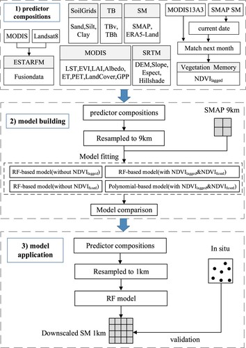
The downscaling process is shown in Figure 2. First, MODIS13A3 data is designed to be NDVI_lagged based on SM time. Subsequently, MODIS and Landsat8 reflectance data are fused using the ESTARFM to generate spatially complete NDVI data. Next, the NDVI_lagged, NDVI_fused, and other variables are resampled to 9 km resolution to match the spatial resolution of SMAP data. NDVI and EVI have similar performance in the RF-based downscaling model (Hu et al. 2020). We used both NDVIlagged and EVI because they can provide vegetation cover conditions in different time scales. NDVIlagged provides vegetation cover conditions after one month of soil moisture. EVI provides vegetation cover status for the most recent 16 days from soil moisture time. The SMAP soil moisture acquisition time served as the baseline for selecting the closest corresponding input data for the model. To investigate the effects of lagged vegetation data and fusion results on the SM downscaling method, we compared the RF-based model without NDVI_lagged and NDVI_fused to models including each, respectively. The models are expressed in Equations (1)–(3). Additionally, a commonly used polynomial statistical regression model with the expression (4) was developed for comparison with the RF models to evaluate their performance. Last, the auxiliary data were resampled to 1 km resolution and fed into the validated RF-based downscaling model to generate high-resolution SM at 1 km. The accuracy of downscaled SM results was assessed using in situ SM at 30 sites within the study area. (1) $\mathrm{SM}=f\left(\begin{array}{c}\mathrm{NDV}{\mathrm{I}}_{\mathrm{lagged}},\mathrm{NDV}{\mathrm{I}}_{\mathrm{fused}},\mathrm{EVI},\mathrm{LAI},\mathrm{LST},\mathrm{ET},\mathrm{PET},\mathrm{GPP},\mathrm{Albedo},\mathrm{Landcover},\\ \mathrm{Tbh},\mathrm{Tbv},\mathrm{elevation},\mathrm{slope},\mathrm{aspect},\mathrm{hillshade},\mathrm{sand},\mathrm{caly},\mathrm{slit},\mathrm{ERA}5\text{-}\mathrm{SM}\end{array}\right)$(1) (2) $\mathrm{SM}=f\left(\begin{array}{c}\mathrm{NDV}{\mathrm{I}}_{\mathrm{lagged}},\mathrm{EVI},\mathrm{LAI},\mathrm{LST},\mathrm{ET},\mathrm{PET},\mathrm{GPP},\mathrm{Albedo},\mathrm{Landcover},\\ \mathrm{Tbh},\mathrm{Tbv},\mathrm{elevation},\mathrm{slope},\mathrm{aspect},\mathrm{hillshade},\mathrm{sand},\mathrm{caly},\mathrm{slit},\mathrm{ERA}5\text{-}\mathrm{SM}\end{array}\right)$(2) (3) $\mathrm{SM}=f\left(\begin{array}{c}\mathrm{NDV}{\mathrm{I}}_{\mathrm{fused}},\mathrm{EVI},\mathrm{LAI},\mathrm{LST},\mathrm{ET},\mathrm{PET},\mathrm{GPP},\mathrm{Albedo},\mathrm{Landcover},\\ \mathrm{Tbh},\mathrm{Tbv},\mathrm{elevation},\mathrm{slope},\mathrm{aspect},\mathrm{hillshade},\mathrm{sand},\mathrm{caly},\mathrm{slit},\mathrm{ERA}5\text{-}\mathrm{SM}\end{array}\right)$(3) (4) $\begin{array}{rl}\mathrm{SM}=& a_{000}+a_{001}\mathrm{EVI}+a_{010}\mathrm{LST}+a_{100}\mathrm{ERA}5\text{-}\mathrm{SM}+a_{002}\mathrm{EV}{\mathrm{I}}^2+a_{020}\mathrm{LS}{\mathrm{T}}^2\\ & +a_{200}\mathrm{ERA}5\text{-}\mathrm{S}{\mathrm{M}}^2+a_{011}\mathrm{EVI}\ast \mathrm{LST}+a_{101}\mathrm{EVI}\ast \mathrm{ERA}5\text{-}\mathrm{SM}+a_{110}\mathrm{LST}\ast \mathrm{ERA}5\text{-}\mathrm{SM}\end{array}$(4) where a_ijk are the regression coefficients.

Figure 2. Flowchart of the SM downscaling method.

3.5. Evaluation method

Statistical metrics are used to quantify errors by comparing the estimated values with reference data. To comprehensively evaluate the accuracy of the best-performing downscaling models, four statistical indicators were adopted, including correlation coefficient (R), root mean square error (RMSE), unbiased root mean square error (ubRMSE), and bias. The calculations for these statistical indicators are provided below: (5) $\mathrm{Bias}={\displaystyle \frac{1}{N}\sum _{i=1}^N\left({\theta }_{\mathrm{satellite}}-{\theta }_{\mathrm{in}\text{-}\mathrm{situ}}\right)}$(5) (6) $\mathrm{RMSE}=\sqrt{{\displaystyle \frac{1}{N}\sum _{i=1}^N{\left({\theta }_{\mathrm{satellite}}-{\theta }_{\mathrm{in}\text{-}\mathrm{situ}}\right)}^2}}$(6) (7) $\mathrm{ubRMSE}=\sqrt{\mathrm{RMS}{\mathrm{E}}^2-\mathrm{Bia}{\mathrm{s}}^2}$(7) (8) $\mathrm{R}={\displaystyle \frac{{\sum \left({\theta }_{\mathrm{in}\text{-}\mathrm{situ}}-\overline{{\theta }_{\mathrm{in}\text{-}\mathrm{situ}}}\right)}^2{\left({\theta }_{\mathrm{satellite}}-\overline{{\theta }_{\mathrm{satellite}}}\right)}^2}{\sqrt{{\sum \left({\theta }_{\mathrm{in}\text{-}\mathrm{situ}}-\overline{{\theta }_{\mathrm{in}\text{-}\mathrm{situ}}}\right)}^2{\left({\theta }_{\mathrm{satellite}}-\overline{{\theta }_{\mathrm{satellite}}}\right)}^2}}}$(8)

4. Results

4.1. Validation of the proposed downscaling method

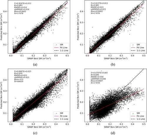
Figure 3 compares the downscaled SM values obtained from RF models trained with different combinations of NDVI_lagged and NDVI_fused to the SMAP SM data. The training and validation dataset contained 35,484 and 17,478 samples, respectively. The scatter diagram demonstrates the superior performance of the RF model incorporating both NDVI_lagged and NDVI_fused (R 0.983) compared to models without NDVI_lagged (R 0.981) or NDVI_fused (R 0.959). Notably, the RF model with both NDVI_lagged and NDVI_fused significantly outperforms the polynomial-based model with both (R 0.686). The RF model with NDVI_lagged and NDVI_fused also exhibits the lowest RMSE and ubRMSE values. Visually, the fitted line of the RF-based models with both NDVI_lagged and NDVI_fused is closer to the 1:1 line in the scatterplot, indicating its superior ability to capture the non-linear relationship between soil moisture and input variables compared to other models. Therefore, the RF-based model with NDVI_lagged and NDVI_fused is chosen for subsequent analyses.

Figure 3. Comparison of downscaled SM against SMAP SM for different models. (a) the RF-based model (with NDVI_lagged&NDVI_fused), (b) the RF-based model (without NDVI_lagged), (c) the RF-based model (without NDVI_fused), (d) the polynomial-based model (with NDVI_lagged&NDVI_fused).

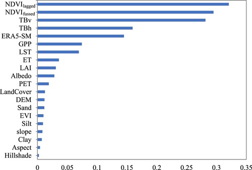
Figure 4 presents the variable importance scores within the downscaling model. We can see that NDVI_lagged and NDVI_fused had the highest score, followed by TBv and TBh. These variables likely contribute the most to error reduction during downscaling. This is due to the significant positive correlation between NDVI and soil moisture, with NDVI typically lagging behind SM by one month (Chen et al. 2014; West et al. 2018). Additionally, fused NDVI offers richer spatial information. TB includes parameters of the Earth's emission at L-band, such as soil roughness, soil texture and soil temperature, etc.

Figure 4. Feature importance scores for the downscaling method.

4.2. Validation of the downscaled SM

To validate the performance of the RF-based model (with NDVI_lagged&NDVI_fused), the downscaled 1 km SM is compared with in situ measurements at 30 stations in Henan province. Figure 5 shows scatter diagrams at different sites. The first and third rows show the original SMAP SM data vs. in situ SM, with the X-axis representing the in situ SM and the Y-axis representing the SMAP SM. The second and fourth rows show downscaled SM data vs. in situ SM, with the X-axis representing the in situ SM and the Y-axis representing the downscaled SM. Meanwhile, Figure 5 shows the values of four statistical indicators, namely, R, RMSE, ubRMSE, and bias, and gives the fitting line of the scatter. The scatterplots for eight stations reveal higher R values between the downscaled SM and in situ measurements compared to the original SMAP SM and in situ measurements. In terms of RMSE, the downscaled SM exhibits lower values at most sites, indicating improved performance compared to the original SMAP data. Similar trends are observed for ubRMSE, and bias values show comparable performance between pre- and post-downscaling SM.

Figure 5. Scatter plots of the original SMAP SM against the in situ SM and downscaled SM of the RF-based model (with NDVI_lagged&NDVI_fused) against the in situ SM at different stations.

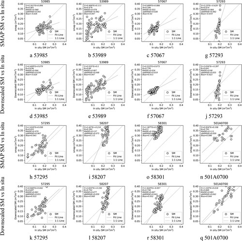
Table 2 shows the detailed statistical metrics between the downscaled SM from the RF-based model (with NDVI_lagged&NDVI_fused) and in situ SM measurements at 30 stations, including R, RMSE, ubRMSE, and Bias, as well as the slope, intercept, and the number of valid data. The statistics indicate successful downscaling with good agreement between the downscaled and observed SM. The correlation coefficient across all stations ranged from 0.628 to 0.849, with an average R of 0.689. The RMSE ranged from 0.024 to 0.094 m³/m³, with an average of 0.057 m³/m³. The ubRMSE values range from 0.019 to 0.060 m³/m³, with an average of 0.043 m³/m³. The Bias values range from −0.085 to 0.057 m³/m³, with an average value of −0.005 m³/m³. Overall, the proposed downscaling models can greatly improve the correlation of downscaled SM and effectively reduce error.

Table 2. Detailed statistical metrics for the downscaled SM of the RF-based model (with NDVI_lagged&NDVI_fused) at 30 sites.

Station	R	RMSE (m^3/m^3)	ubRMSE (m^3/m^3)	Bias (m^3/m^3)	a	b
53889	0.653	0.065	0.030	0.057	0.535	0.101
53985	0.636	0.044	0.034	−0.028	0.409	0.079
53989	0.660	0.067	0.048	0.047	0.555	0.100
53993	0.677	0.042	0.029	0.030	0.601	0.072
57066	0.633	0.027	0.027	0.006	0.553	0.071
57067	0.739	0.024	0.019	0.015	0.533	0.073
57099	0.657	0.067	0.040	−0.054	0.758	−0.014
57162	0.681	0.044	0.034	−0.028	0.415	0.073
57177	0.645	0.061	0.046	−0.040	2.022	−0.238
57178	0.628	0.055	0.055	−0.003	0.525	0.055
57187	0.644	0.085	0.056	−0.065	0.549	0.014
57290	0.708	0.047	0.044	0.017	1.471	−0.049
57293	0.641	0.060	0.055	−0.023	3.034	−0.397
57295	0.697	0.061	0.051	0.033	0.946	0.042
57296	0.694	0.058	0.052	0.026	0.691	0.093
58207	0.752	0.077	0.059	0.049	2.655	−0.336
58301	0.738	0.067	0.041	0.052	1.624	−0.057
O2073	0.678	0.043	0.037	0.022	0.540	0.078
O2081	0.661	0.034	0.031	0.015	0.518	0.077
O2176	0.724	0.051	0.030	−0.041	0.455	0.060
O2422	0.636	0.049	0.049	0.006	1.468	−0.055
O2519	0.660	0.059	0.045	−0.038	0.904	−0.017
O4279	0.676	0.051	0.051	−0.004	0.300	0.108
O5291	0.673	0.058	0.037	−0.045	0.605	0.025
501A0500	0.826	0.050	0.048	0.012	1.682	−0.155
501A0700	0.849	0.061	0.042	0.044	1.103	0.018
502A2700	0.713	0.080	0.060	−0.052	1.950	−0.301
502A3500	0.753	0.039	0.037	0.010	0.752	0.069
508A2700	0.686	0.090	0.048	−0.077	2.815	−0.403
620A7800	0.659	0.094	0.040	−0.085	1.268	−0.152
Mean	0.689	0.057	0.043	−0.005	1.075	−0.032

Inevitably, there are differences between the in situ SM and the downscaled SM. This is due to the fact that soil moisture variations are influenced by numerous variables, such as temperature, vegetation, topography, soil texture, and albedo. Additionally, the study areas exhibit complex environmental conditions that affect SM distribution. Furthermore, soil water evapotranspiration varies considerably due to vegetation cover, climatic conditions, and irrigation scheduling, leading to spatial variations in soil moisture. Meanwhile, the observation stations represent the soil moisture at a specific location, whereas the downscaled SM is raster images with a spatial resolution of 1 km, representing the average soil moisture within that area. Because of the spatial inconsistency between the point-based observation and 1 km resolution downscaled SM, unreasonable deviations are inevitable.

4.3. Spatial patterns of downscaled soil moisture

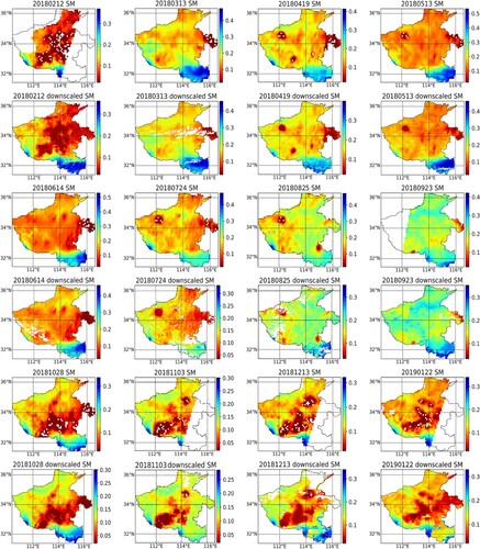
To evaluate the performance of the spatial distributions in downscaled soil moisture, Figure 6 compares the spatial variations of the downscaled SM using the RF-based model to the original coarse-resolution SMAP SM across consecutive months from February 2018 to January 2019. The first, third, and fifth rows show the raw SMAP SM, and the second, fourth and sixth rows depict the downscaled SM at the same time. It can be found that the proposed downscaling model using the RF model with NDVI_lagged and NDVI_fused demonstrates effectiveness in generating 1 km spatial resolution SM data. The spatial distribution of the downscaled SM exhibits highly consistent with the original SMAP SM. Notably, the original SMAP can not always completely cover the study area due to the limitation in satellite scan width. In addition, cloud contamination disrupts optical data within the downscaling auxiliary factors, and the pixels with poor quality are removed during preprocessing, further limiting the effective coverage of SM. Moreover, the downscaled SM reveals more detailed information on spatial variability compared to the original SMAP SM. The pre-downscaling data possesses low spatial resolution, with the same value assigned to each 36 km resolution pixel, leading to abrupt changes in adjacent SM values. Conversely, the downscaled SM boasts a 1 km resolution, resulting in more natural transitions between neighboring SM values. The comparison of soil moisture before and after downscaling highlights the model's ability to generate high-resolution SM that accurately reflects the spatial distribution of SM.

Figure 6. Spatial comparisons of the original SMAP SM and downscaled SM

4.4. Temporal variability of downscaled soil moisture

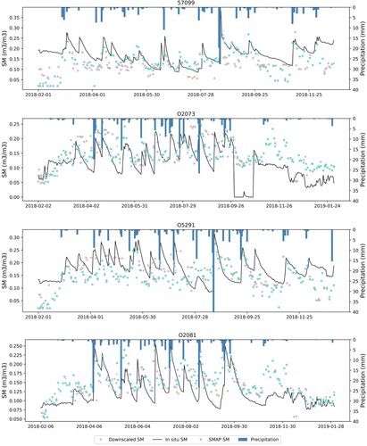
To further analyze the temporal variation of the downscaled SM, dynamic changes of original SM, downscaled SM, in situ SM measurements, and daily precipitation are plotted for four selected stations, spanning February 2018 to February 2019 (Figure 7). The downscaled SM exhibits good temporal consistency with the original SMAP SM. Both datasets generally capture the temporal variations observed in the in situ SM measurements across different stations. Compared to the SMAP SM, the downscaled SM exhibits a closer alignment with the in situ SM measurements at different locations. Simultaneously, the downscaled SM displays are highly correlated with daily precipitation data. Precipitation events mainly occurred in July, August, and September, with relatively high precipitation values corresponding to periods of relatively high SM, and there was a significant increase in SM after the precipitation occurred.

Figure 7. Temporal variations of original SMAP SM, downscaled SM, in situ SM measurements, and daily precipitation during February 2018 – February 2019 at four selected stations

5. Discussion

5.1. Contributions of vegetation memory to the performance of SM downscaling

In this section, we evaluate the contributions of NDVI_lagged to SM downscaling using in situ measurements from 30 stations. Table 3 shows the scatter plot of downscaled SM without NDVI_lagged versus the in situ measurements. As shown in Tables 1 and 2, the RF model with NDVI_lagged data can improve the accuracy of downscaled SM compared to the RF model without NDVI_lagged data. The mean R for the RF model with NDVI_lagged data is 0.689, while the mean R for the RF model without NDVI_lagged data is 0.398, representing a 73% increase. Similarly, the RMSE and ubRMSE metrics decreased by 16% and 30%, respectively.

Table 3. Statistical metrics of the downscaled SM without NDVI_lagged at 30 sites.

Station	R	RMSE (m^3/m^3)	ubRMSE (m^3/m^3)	Bias (m^3/m^3)	a	b
53889	0.480	0.068	0.040	0.056	0.459	0.105
53985	0.224	0.057	0.055	−0.016	0.241	0.116
53989	0.507	0.078	0.058	0.052	0.505	0.112
53993	0.524	0.052	0.039	0.035	0.501	0.089
57066	−0.017	0.060	0.057	0.019	−0.025	0.168
57067	0.215	0.041	0.037	0.018	0.242	0.114
57099	0.353	0.067	0.046	−0.049	0.330	0.064
57162	0.290	0.059	0.058	−0.013	0.331	0.102
57177	0.566	0.053	0.047	−0.024	1.762	−0.171
57178	0.332	0.079	0.075	0.024	0.286	0.109
57187	0.250	0.095	0.084	−0.044	0.232	0.095
57290	0.364	0.057	0.052	0.024	0.752	0.059
57293	0.399	0.045	0.045	−0.002	1.432	−0.081
57295	0.434	0.072	0.062	0.036	0.422	0.122
57296	0.724	0.053	0.051	0.013	0.669	0.083
58207	0.474	0.082	0.078	−0.023	1.890	−0.228
58301	0.582	0.057	0.053	0.023	1.502	−0.066
O2073	0.614	0.055	0.046	0.031	0.684	0.070
O2081	0.477	0.040	0.037	0.016	0.402	0.093
O2176	0.302	0.061	0.053	−0.030	0.305	0.097
O2422	0.349	0.062	0.056	0.027	0.766	0.057
O2519	0.444	0.065	0.054	−0.036	0.585	0.054
O4279	−0.012	0.078	0.078	−0.006	−0.009	0.159
O5291	0.393	0.063	0.055	−0.030	0.462	0.066
501A0500	0.521	0.067	0.058	−0.033	1.008	−0.035
501A0700	0.480	0.078	0.077	−0.011	0.670	0.070
502A2700	0.300	0.094	0.063	−0.070	0.652	0.019
502A3500	0.481	0.071	0.061	−0.037	0.597	0.064
508A2700	0.471	0.069	0.059	−0.036	2.101	−0.234
620A7800	0.414	0.093	0.049	−0.079	0.821	−0.034
Mean	0.398	0.066	0.056	−0.005	0.686	0.041

The primary contribution of applying NDVI_lagged is to enrich the time scale of vegetation data in the input data, ultimately enhancing the accuracy of downscaled soil moisture. It is important to note that the optimal lag time for capturing the strongest NDVI-soil moisture correlation may vary depending on land cover types (Musyimi 2011). However, a one-month lag time aligns with the monthly operational cycle of many agricultural drought monitoring activities (Han et al. 2014). Besides, we use the same NDVI_lagged at both the beginning and end of each month during downscaling. Therefore, there are big temporal inconsistencies within the downscaling process, making it challenging to quantify the exact time difference.

5.2. Contributions of fused NDVIto the performance of SM downscaling

In this section, the in situ measurements of 30 stations were selected to assess the contributions of NDVI_fused in SM downscaling. Table 4 shows the scatter plot of downscaled SM without NDVI_fused applied versus the in situ measurements. As can be seen from Tables 1 to 3, the RF model with NDVI_fused data exhibits improved downscaled SM accuracy compared to the RF model without NDVI_fused data. The RF model without NDVI_fused data had an average R of 0.327, representing an increase (110%) in R value when NDVI_fused is included (0.689). Similarly, improvements are observed for the RMSE and ubRMSE metrics, with a decrease of 40% and 65%, respectively.

Table 4. Statistical metrics of the downscaled SM without NDVI_fused at 30 sites.

Station	R	RMSE(m^3/m^3)	ubRMSE(m^3/m^3)	Bias(m^3/m^3)	a	b
53889	0.424	0.091	0.054	0.073	0.603	0.110
53985	0.215	0.071	0.071	0.000	0.340	0.115
53989	0.435	0.105	0.076	0.072	0.592	0.121
53993	0.539	0.071	0.050	0.050	0.786	0.074
57066	−0.057	0.085	0.078	0.033	−0.124	0.196
57067	0.109	0.056	0.051	0.024	0.178	0.128
57099	0.280	0.070	0.048	−0.051	0.260	0.073
57162	0.282	0.077	0.077	0.006	0.472	0.097
57177	0.445	0.062	0.061	−0.013	1.683	−0.145
57178	0.208	0.105	0.097	0.041	0.248	0.131
57187	0.168	0.108	0.105	−0.026	0.211	0.117
57290	0.268	0.087	0.075	0.044	0.780	0.075
57293	0.276	0.067	0.064	0.020	1.370	−0.048
57295	0.379	0.094	0.075	0.056	0.476	0.134
57296	0.686	0.055	0.055	0.008	0.652	0.081
58207	0.432	0.088	0.084	−0.026	1.813	−0.213
58301	0.476	0.059	0.056	0.019	1.244	−0.024
O2073	0.578	0.078	0.062	0.047	0.903	0.059
O2081	0.508	0.051	0.042	0.028	0.599	0.079
O2176	0.267	0.070	0.068	−0.016	0.387	0.096
O2422	0.186	0.092	0.079	0.047	0.553	0.103
O2519	0.319	0.078	0.077	−0.012	0.588	0.078
O4279	−0.107	0.096	0.096	0.010	−0.110	0.191
O5291	0.314	0.076	0.074	−0.015	0.516	0.071
501A0500	0.486	0.071	0.070	−0.010	1.100	−0.034
501A0700	0.379	0.085	0.084	0.008	0.537	0.122
502A2700	0.174	0.096	0.083	−0.048	0.484	0.085
502A3500	0.367	0.076	0.068	−0.035	0.468	0.098
508A2700	0.473	0.087	0.086	−0.012	3.000	−0.371
620A7800	0.288	0.093	0.074	−0.056	0.823	−0.011
Mean	0.327	0.080	0.071	0.009	0.714	0.053

The primary contribution of applying NDVI_fused is to improve spatial completeness and provide more detailed vegetation characteristics, in addition to enhancing the accuracy of downscaled soil moisture. LST is another crucial factor in SM downscaling. Several studies have explored LST reconstruction methods to decrease cloud cover's influence and increase the available data under clear sky (Zeng et al. 2018; Zhao and Duan 2020; Zhu et al. 2022). We found that many studies used MOD11A1 as a downscaling factor (Hu et al. 2020; Mao et al. 2022; Xu et al. 2022). In this study, we primarily focused on increasing available NDVI through ESTARFM, potentially neglecting the clouds effect on LST.

5.3. Advantages and limitations of this study

Due to the effects of lagged vegetation data on soil moisture, we propose the RF model that considers vegetation memory and spatiotemporal fusion to produce 1 km × 1 km SM. The key advantages are as follows. First, the downscaling method considers the time lag between vegetation and soil moisture, and we used NDVI which lags behind SM by 1 month as one of the input data to the model. The reason for considering NDVI_lagged data is that many studies (Chen et al. 2014; McNally et al. 2016; Sur et al. 2020) used multi-year monthly data to analyze the relationship between soil moisture and vegetation, typically finding a one-month lag between NDVI and surface soil moisture. Second, the downscaling method also incorporates high-resolution (30 m) NDVI_fused using the ESTARFM algorithm. The fused NDVI overcomes the limitations associated with cloud-contaminated optical sensors and provides richer vegetation information. Last, beyond commonly used NDVI and LST data, the input data encompass various additional features (20 in total) including land use, topography, soil properties, SMAP bright temperature, evapotranspiration, etc. The features significantly impact the spatial and temporal distribution of soil moisture (Famiglietti et al. 2008) and can provide a valuable reference for SM downscaling. The results achieved comparable performance to other studies (Hu et al. 2020; Mishra et al. 2018; Zhao et al. 2022). In conclusion, the downscaling methods consider vegetation memory and increase the amount of vegetation data by spatiotemporal fusion, which improves the accuracy of downscaled SM products.

It is necessary to outline the limitations of the RF models in this study. Firstly, While SMAP TB data is of high importance for soil moisture, its coarser spatial resolution compared to other input variables might influence model accuracy. Nonetheless, SMAP TB data can provide valuable information on bright temperatures for downscale SM (Bai et al. 2019; Hu et al. 2020). Secondly, beyond the variables used in this article, there are many other variables related to soil moisture, such as several days’ time-lagged values for the daily rainfall, air temperature, and soil moisture (Kwon, Kwon, and Han 2018; Mao et al. 2022). In addition, temporal discrepancies exist between various input variables and SMAP data. For instance, the orbital revisit times of Terra and Aqua satellites differ from SMAP, introducing potential errors. Nevertheless, MODIS data provide high spatial resolution information valuable for the downscaled method (Amazirh, Merlin, and Er-Raki 2019; El Hajj et al. 2017). Lastly, the in situ measurements estimate SM at depths of 10 cm, whereas the SMAP estimated the soil moisture at depths of 5 cm. Furthermore, the downscaled SM has a 1 km spatial resolution, contrasting with the point-based nature of in situ observations. These inconsistencies in depth and spatial resolution inevitably lead to some discrepancies in validation statistics. Despite all this, some studies also used in situ measurements at depths of 10 cm for SM validation (Lacava et al. 2012; Peng et al. 2015; Sun et al. 2017).

6. Conclusion

This study presents a machine-learning approach for downscaling SMAP soil moisture (SM) that incorporates vegetation memory and spatiotemporal fusion. The method utilizes multi-source remote sensing data, including SMAP, MODIS, ERA5-land, and so on. This study successfully generated SM at 1 km × 1 km with acceptable performance when compared to the in situ measurements. Moreover, the contributions of NDVI_lagged and NDVI_fused for improving the accuracy of downscaling SM were thoroughly explored. The major conclusions are given as follows:

1. The downscaled SM using the RF-based model with NDVI_lagged outperformed that without NDVI_lagged. The inclusion of NDVI_lagged increased the average R by 73% and decreased the RMSE by 16%. The contributions of NDVI_lagged were mainly in enriching the time scale of vegetation indices data in the input data of the model and improving the accuracy of downscaled soil moisture.

2. The downscaled SM using the RF-based model with NDVI_fused outperformed that without NDVI_fused. The inclusion of NDVI_fused increased the average R by 110% and decreased the RMSE by 40%. The contribution of NDVI_fused was mainly in improving spatial completeness and providing more detailed vegetation information.

3. The RF method considering both vegetation memory and spatiotemporal fusion can improve the performance of the downscaled SM significantly. The RF method with NDVI_lagged&NDVI_fused has the highest R of 0.983 and the lowest RMSE of 0.014 m³/m³, which is better than the RF method without NDVI_lagged (R of 0.981, RMSE of 0.015 m³/m³), surpassing the RF method without NDVI_fused (R of 0.959, RMSE of 0.023 m³/m³). The performance of these RF models is all better than the polynomial downscaling model with NDVI_lagged&NDVI_fused, which has the lowest R of 0.686 and highest RMSE of 0.056 m³/m³.

4. The RF model exhibited good performance in generating SM estimates that are highly consistent with in situ SM measurements. The correlation coefficients range from 0.628 to 0.849 across all stations, with an average R of 0.689. The RMSE ranges from 0.024 to 0.094 m³/m³ with an average of 0.057 m³/m³. In terms of R and RMSE, the results are comparable to existing studies (Hu et al. 2020; Zhao et al. 2018), which basically meets the SMAP task accuracy target. The average ubRMSE across all stations is 0.042 m³/m³, and the average bias is –0.014 m³/m³.

In conclusion, the proposed method effectively leverages machine learning algorithms, spatiotemporal fusion, and vegetation memory data to downscale SM. This approach demonstrates promising applications in Henan Province, an important agricultural region in China. The improved SM data holds significant value for regional hydrological studies and agricultural applications. Looking ahead, advancements in artificial intelligence and satellite observation technologies offer exciting possibilities. Future research could integrate fine-scale remote sensing data to develop field scales (30 m × 30 m) and temporally continuous (daily) SM products across heterogeneous land surfaces.

Acknowledgements

We would like to thank the anonymous reviewers and journal editors for their constructive and valuable suggestions to improve the quality of this article.

Disclosure statement

No potential conflict of interest was reported by the author(s).

Data availability statement

The data that support the findings of this study are available from the corresponding author upon reasonable request.

Additional information

Funding

This work was supported by the National Key Research and Development Program of China [grant number 2021YFB3900603].

References

- Abowarda, A. S., L. L. Bai, C. J. Zhang, D. Long, X. Y. Li, Q. Huang, and Z. L. Sun. 2021. “Generating Surface Soil Moisture at 30 m Spatial Resolution Using Both Data Fusion and Machine Learning Toward Better Water Resources Management at the Field Scale.” Remote Sensing of Environment 255: 112301. https://doi.org/10.1016/j.rse.2021.112301.
- Amazirh, A., O. Merlin, and S. Er-Raki. 2019. “Including Sentinel-1 Radar Data to Improve the Disaggregation of MODIS Land Surface Temperature Data.” ISPRS Journal of Photogrammetry and Remote Sensing 150:11–26. https://doi.org/10.1016/j.isprsjprs.2019.02.004.
- Bai, Jueying, Qian Cui, Wen Zhang, and Lingkui Meng. 2019. “An Approach for Downscaling SMAP Soil Moisture by Combining Sentinel-1 SAR and MODIS Data.” Remote Sensing 11 (23): 2736. https://doi.org/10.3390/rs11232736.
- Bhuiyan, H. A. K. M., H. McNairn, J. Powers, M. Friesen, A. Pacheco, T. J. Jackson, M. H. Cosh, et al. 2018. “Assessing SMAP Soil Moisture Scaling and Retrieval in the Carman (Canada) Study Site.” Vadose Zone Journal 17 (1): 1–14. https://doi.org/10.2136/vzj2018.07.0132.
- Bolten, J. D., and W. T. Crow. 2012. “Improved Prediction of Quasi-Global Vegetation Conditions Using Remotely-Sensed Surface Soil Moisture.” Geophysical Research Letters 39 (19): 39. https://doi.org/10.1029/2012gl053470.
- Breiman, L. 2001. “Random Forests.” Machine Learning 45 (1): 5–32. https://doi.org/10.1023/A:1010933404324.
- Brocca, L., W. Zhao, and H. Lu. 2023. “High-Resolution Observations from Space to Address New Applications in Hydrology.” Innovation (Camb) 4 (3): 100437. https://doi.org/10.1016/j.xinn.2023.100437.
- Chanasyk, D. S., and M. A. Naeth. 1996. “Field Measurement of Soil Moisture Using Neutron Probes.” Canadian Journal of Soil Science 76: 317–323. https://doi.org/10.4141/cjss96-038.
- Chang, Li-Ling, Ravindra Dwivedi, John F. Knowles, Yuan-Hao Fang, Guo-Yue Niu, Jon D. Pelletier, Craig Rasmussen, Matej Durcik, Greg A. Barron-Gafford, and Thomas Meixner. 2018. “Why Do Large-Scale Land Surface Models Produce a Low Ratio of Transpiration to Evapotranspiration?” Journal of Geophysical Research: Atmospheres 123 (17): 9109–9130. https://doi.org/10.1029/2018JD029159.
- Chen, T., R. A. M. de Jeu, Y. Y. Liu, G. R. van der Werf, and A. J. Dolman. 2014. “Using Satellite Based Soil Moisture to Quantify the Water Driven Variability in NDVI: A Case Study Over Mainland Australia.” Remote Sensing of Environment 140:330–338. https://doi.org/10.1016/j.rse.2013.08.022.
- Chen, S. D., D. X. She, L. P. Zhang, M. Y. Guo, and X. Liu. 2019. “Spatial Downscaling Methods of Soil Moisture Based on Multisource Remote Sensing Data and Its Application.” Water 11 (7): 1401. https://doi.org/10.3390/w11071401.
- Chen, Yong, and Huiling Yuan. 2020. “Evaluation of Nine Sub-Daily Soil Moisture Model Products Over China Using High-Resolution in Situ Observations.” Journal of Hydrology 588: 125054. https://doi.org/10.1016/j.jhydrol.2020.125054.
- Chen, Yi, Zhao Zhang, and Fulu Tao. 2018. “Improving Regional Winter Wheat Yield Estimation Through Assimilation of Phenology and Leaf Area Index from Remote Sensing Data.” European Journal of Agronomy 101:163–173. https://doi.org/10.1016/j.eja.2018.09.006.
- Coenders-Gerrits, A. M., R. J. van der Ent, T. A. Bogaard, L. Wang-Erlandsson, M. Hrachowitz, and H. H. Savenije. 2014. “Uncertainties in Transpiration Estimates.” Nature 506 (7487): E1–E2. https://doi.org/10.1038/nature12925.
- Dai, Yongjiu, Wei Shangguan, Nan Wei, Qinchuan Xin, Hua Yuan, Shupeng Zhang, Shaofeng Liu, Xingjie Lu, Dagang Wang, and Fapeng Yan. 2019. “A Review of the Global Soil Property Maps for Earth System Models.” Soil 5 (2): 137–158. https://doi.org/10.5194/soil-5-137-2019.
- Djamai, N., R. Magagi, K. Goita, O. Merlin, Y. Kerr, and A. Roy. 2016. “A Combination of DISPATCH Downscaling Algorithm with CLASS Land Surface Scheme for Soil Moisture Estimation at Fine Scale During Cloudy Days.” Remote Sensing of Environment 184:1–14. https://doi.org/10.1016/j.rse.2016.06.010.
- Ebrahimi-Khusfi, M., S. K. Alavipanah, S. Hamzeh, F. Amiraslani, N. N. Samany, and J. P. Wigneron. 2018. “Comparison of Soil Moisture Retrieval Algorithms Based on the Synergy Between SMAP and SMOS-IC.” International Journal of Applied Earth Observation and Geoinformation 67:148–160. https://doi.org/10.1016/j.jag.2017.12.005.
- El Hajj, M., N. Baghdadi, M. Zribi, and H. Bazzi. 2017. “Synergic Use of Sentinel-1 and Sentinel-2 Images for Operational Soil Moisture Mapping at High Spatial Resolution Over Agricultural Areas.” Remote Sensing 9 (12): 1292. https://doi.org/10.3390/rs9121292.
- Engstrom, Ryan, Allen Hope, Hyojung Kwon, and Douglas Stow. 2008. “The Relationship Between Soil Moisture and NDVI Near Barrow, Alaska.” Physical Geography 29 (1): 38–53. https://doi.org/10.2747/0272-3646.29.1.38.
- Famiglietti, James S., Dongryeol Ryu, Aaron A. Berg, Matthew Rodell, and Thomas J. Jackson. 2008. “Field Observations of Soil Moisture Variability Across Scales.” Water Resources Research 44 (1): W01423. https://doi.org/10.1029/2006wr005804.
- Fan, Xinyi, Peng Gao, Biqing Tian, Changxue Wu, and Xingmin Mu. 2023. “Spatio-Temporal Patterns of NDVI and Its Influencing Factors Based on the ESTARFM in the Loess Plateau of China.” Remote Sensing 15 (10): 2553. https://doi.org/10.3390/rs15102553.
- Fisher, R. A., and C. D. Koven. 2020. “Perspectives on the Future of Land Surface Models and the Challenges of Representing Complex Terrestrial Systems.” Journal of Advances in Modeling Earth Systems 12 (4): e2018MS001453. https://doi.org/10.1029/2018MS001453.
- Gessner, U., V. Naeimi, I. Klein, C. Kuenzer, D. Klein, and S. Dech. 2013. “The Relationship Between Precipitation Anomalies and Satellite-Derived Vegetation Activity in Central Asia.” Global and Planetary Change 110:74–87. https://doi.org/10.1016/j.gloplacha.2012.09.007.
- Han, Eunjin, Wade T. Crow, Thomas Holmes, and John Bolten. 2014. “Benchmarking a Soil Moisture Data Assimilation System for Agricultural Drought Monitoring.” Journal of Hydrometeorology 15 (3): 1117–1134. https://doi.org/10.1175/JHM-D-13-0125.1.
- Hu, Fengmin, Zushuai Wei, Wen Zhang, Donyu Dorjee, and Lingkui Meng. 2020. “A Spatial Downscaling Method for SMAP Soil Moisture Through Visible and Shortwave-Infrared Remote Sensing Data.” Journal of Hydrology 590: 125360. https://doi.org/10.1016/j.jhydrol.2020.125360.
- Kwon, Moonhyuk, Hyun-Han Kwon, and Dawei Han. 2018. “A Spatial Downscaling of Soil Moisture from Rainfall, Temperature, and AMSR2 Using a Gaussian-Mixture Nonstationary Hidden Markov Model.” Journal of Hydrology 564:1194–1207. https://doi.org/10.1016/j.jhydrol.2017.12.015.
- Lacava, T., L. Brocca, M. Faruolo, P. Matgen, T. Moramarco, N. Pergola, and V. Tramutoli. 2012. “A Multi-Sensor (SMOS, AMSR-E and ASCAT) Satellite-Based Soil Moisture Products Inter-Comparison.” Paper presented at the 2012 IEEE International Geoscience and Remote Sensing Symposium, 22-27 July 2012.
- Lievens, H., S. K. Tomer, A. Al Bitar, G. J. M. De Lannoy, M. Drusch, G. Dumedah, H. J. H. Franssen, et al. 2015. “SMOS Soil Moisture Assimilation for Improved Hydrologic Simulation in the Murray Darling Basin, Australia.” Remote Sensing of Environment 168:146–162. https://doi.org/10.1016/j.rse.2015.06.025.
- Lindell, D. B., and D. G. Long. 2016. “High-Resolution Soil Moisture Retrieval with ASCAT.” IEEE Geoscience and Remote Sensing Letters 13 (7): 972–976. https://doi.org/10.1109/LGRS.2016.2557321.
- Liu, L. B., L. Gudmundsson, M. Hauser, D. H. Qin, S. C. Li, and S. I. Seneviratne. 2020. “Soil Moisture Dominates Dryness Stress on Ecosystem Production Globally.” Nature Communications 11 (1): 4892. https://doi.org/10.1038/s41467-020-18631-1.
- Long, Di, Liangliang Bai, La Yan, Caijin Zhang, Wenting Yang, Huimin Lei, Jinling Quan, Xianyong Meng, and Chunxiang Shi. 2019. “Generation of Spatially Complete and Daily Continuous Surface Soil Moisture of High Spatial Resolution.” Remote Sensing of Environment 233: 111364. https://doi.org/10.1016/j.rse.2019.111364.
- Lopatin, J., K. Dolos, H. J. Hernandez, M. Galleguillos, and F. E. Fassnacht. 2016. “Comparing Generalized Linear Models and Random Forest to Model Vascular Plant Species Richness Using LiDAR Data in a Natural Forest in Central Chile.” Remote Sensing of Environment 173: 200–210. https://doi.org/10.1016/j.rse.2015.11.029.
- Mao, T. N., W. Shangguan, Q. L. Li, L. Li, Y. Zhang, F. N. Huang, J. D. Li, W. Liu, and R. Q. Zhang. 2022. “A Spatial Downscaling Method for Remote Sensing Soil Moisture Based on Random Forest Considering Soil Moisture Memory and Mass Conservation.” Remote Sensing 14 (16): 3858. https://doi.org/10.3390/rs14163858.
- McNally, A., S. Shukla, K. R. Arsenault, S. Wang, C. D. Peters-Lidard, and J. P. Verdin. 2016. “Evaluating ESA CCI Soil Moisture in East Africa.” International Journal of Applied Earth Observation and Geoinformation 48:96–109. https://doi.org/10.1016/j.jag.2016.01.001.
- Meng, S. S., X. H. Xie, and S. L. Liang. 2017. “Assimilation of Soil Moisture and Streamflow Observations to Improve Flood Forecasting with Considering Runoff Routing Lags.” Journal of Hydrology 550:568–579. https://doi.org/10.1016/j.jhydrol.2017.05.024.
- Merlin, O., M. J. Escorihuela, M. A. Mayoral, O. Hagolle, A. Al Bitar, and Y. Kerr. 2013. “Self-Calibrated Evaporation-Based Disaggregation of SMOS Soil Moisture: An Evaluation Study at 3 km and 100 m Resolution in Catalunya, Spain” Remote Sensing of Environment 130:25–38. https://doi.org/10.1016/j.rse.2012.11.008.
- Mimeau, L., Y. Tramblay, L. Brocca, C. Massari, S. Camici, and P. Finaud-Guyot. 2021. “Modeling the Response of Soil Moisture to Climate Variability in the Mediterranean Region.” Hydrology and Earth System Sciences 25 (2): 653–669. https://doi.org/10.5194/hess-25-653-2021.
- Mishra, Vikalp, W. Lee Ellenburg, Robert E. Griffin, John R. Mecikalski, James F. Cruise, Christopher R. Hain, and Martha C. Anderson. 2018. “An Initial Assessment of a SMAP Soil Moisture Disaggregation Scheme Using TIR Surface Evaporation Data Over the Continental United States.” International Journal of Applied Earth Observation and Geoinformation 68:92–104. https://doi.org/10.1016/j.jag.2018.02.005.
- Mladenova, I. E., J. D. Bolten, W. Crow, N. Sazib, and C. Reynolds. 2020. “Agricultural Drought Monitoring via the Assimilation of SMAP Soil Moisture Retrievals into a Global Soil Water Balance Model.” Frontiers in Big Data 3: 10. https://doi.org/10.3389/fdata.2020.00010.
- Mladenova, I. E., T. J. Jackson, E. Njoku, R. Bindlish, S. Chan, M. H. Cosh, T. R. H. Holmes, et al. 2014. “Remote Monitoring of Soil Moisture Using Passive Microwave-Based Techniques – Theoretical Basis and Overview of Selected Algorithms for AMSR-E.” Remote Sensing of Environment 144:197–213. https://doi.org/10.1016/j.rse.2014.01.013.
- Muñoz-Sabater, J., E. Dutra, A. Agustí-Panareda, C. Albergel, G. Arduini, G. Balsamo, S. Boussetta, et al. 2021. “ERA5-Land: A State-of-the-art Global Reanalysis Dataset for Land Applications.” Earth System Science Data 13 (9): 4349–4383. https://doi.org/10.5194/essd-13-4349-2021.
- Musyimi, Z. 2011. “Temporal Relationships Between Remotely-Sensed Soil Moisture and NDVI Over Africa: Potential for Drought Early Warning.” Master's Thesis. Enschede, Netherlands: Dept. of Geo-Information Science and Technology, University of Twenty.
- Peng, Jian, Alexander Loew, Olivier Merlin, and Niko E. C. Verhoest. 2017. “A Review of Spatial Downscaling of Satellite Remotely Sensed Soil Moisture.” Reviews of Geophysics 55 (2): 341–366. https://doi.org/10.1002/2016RG000543.
- Peng, J., J. Niesel, A. Loew, S. Q. Zhang, and J. Wang. 2015. “Evaluation of Satellite and Reanalysis Soil Moisture Products Over Southwest China Using Ground-Based Measurements.” Remote Sensing 7 (11): 15729–15747. https://doi.org/10.3390/rs71115729.
- Qin, J., K. Yang, N. Lu, Y. Y. Chen, L. Zhao, and M. L. Han. 2013. “Spatial Upscaling of in-Situ Soil Moisture Measurements Based on MODIS-Derived Apparent Thermal Inertia.” Remote Sensing of Environment 138:1–9. https://doi.org/10.1016/j.rse.2013.07.003.
- Robock, A., K. Y. Vinnikov, G. Srinivasan, J. K. Entin, S. E. Hollinger, N. A. Speranskaya, S. X. Liu, and A. Namkhai. 2000. “The Global Soil Moisture Data Bank.” Bulletin of the American Meteorological Society 81 (6): 1281–1299. https://doi.org/10.1175/1520-0477(2000)081<1281:Tgsmdb>2.3.Co;2.
- Sahoo, A. K., G. J. M. De Lannoy, R. H. Reichle, and P. R. Houser. 2013. “Assimilation and Downscaling of Satellite Observed Soil Moisture Over the Little River Experimental Watershed in Georgia, USA.” Advances in Water Resources 52:19–33. https://doi.org/10.1016/j.advwatres.2012.08.007.
- Schmugge, T., T. J. Jackson, and H. L. McKim. 1980. “Survey of Methods for Soil Moisture Determination.” Water Resources Research 16 (6): 961–979. https://doi.org/10.1029/WR016i006p00961.
- Shi, Benlin, Xinyu Zhu, Yunchuan Hu, and Yanyan Yang. 2017. “Drought Characteristics of Henan Province in 1961–2013 Based on Standardized Precipitation Evapotranspiration Index.” Journal of Geographical Sciences 27 (3): 311–325. https://doi.org/10.1007/s11442-017-1378-4.
- Sun, Y. Y., S. F. Huang, J. W. Ma, J. R. Li, X. T. Li, H. Wang, S. Chen, and W. B. Zang. 2017. “Preliminary Evaluation of the SMAP Radiometer Soil Moisture Product Over China Using In Situ Data.” Remote Sensing 9 (3): 292. https://doi.org/10.3390/rs9030292.
- Sur, Chanyang, Do-Hyuk Kang, Kyoung Jae Lim, Jae E. Yang, Yongchul Shin, and Younghun Jung. 2020. “Soil Moisture–Vegetation–Carbon Flux Relationship Under Agricultural Drought Condition Using Optical Multispectral Sensor.” Remote Sensing 12 (9): 1359. https://doi.org/10.3390/rs12091359.
- Tao, Guofeng, Kun Jia, Xiangqin Wei, Mu Xia, Bing Wang, Xianhong Xie, Bo Jiang, Yunjun Yao, and Xiaotong Zhang. 2021. “Improving the Spatiotemporal Fusion Accuracy of Fractional Vegetation Cover in Agricultural Regions by Combining Vegetation Growth Models.” International Journal of Applied Earth Observation and Geoinformation 101: 102362. https://doi.org/10.1016/j.jag.2021.102362.
- van Hateren, Theresa C., Marco Chini, Patrick Matgen, and Adriaan J. Teuling. 2021. “Ambiguous Agricultural Drought: Characterising Soil Moisture and Vegetation Droughts in Europe from Earth Observation.” Remote Sensing 13 (10): 1990. https://doi.org/10.3390/rs13101990.
- Wang, Y. A., X. Fu, D. M. Wu, M. D. Wang, K. D. Lu, Y. J. Mu, Z. G. Liu, Y. H. Zhang, and T. Wang. 2021. “Agricultural Fertilization Aggravates Air Pollution by Stimulating Soil Nitrous Acid Emissions at High Soil Moisture.” Environmental Science & Technology 55 (21): 14556–14566. https://doi.org/10.1021/acs.est.1c04134.
- Wang, Aihui, and Xueli Shi. 2019. “A Multilayer Soil Moisture Dataset Based on the Gravimetric Method in China and Its Characteristics.” Journal of Hydrometeorology 20 (8): 1721–1736. https://doi.org/10.1175/JHM-D-19-0035.1.
- Wang, Shuai, Chaozi Wang, Chenglong Zhang, Jingyuan Xue, Pu Wang, Xingwang Wang, Weishu Wang, et al. 2022. “A Classification-Based Spatiotemporal Adaptive Fusion Model for the Evaluation of Remotely Sensed Evapotranspiration in Heterogeneous Irrigated Agricultural Area.” Remote Sensing of Environment 273: 112962. https://doi.org/10.1016/j.rse.2022.112962.
- West, H., N. Quinn, M. Horswell, and P. White. 2018. “Assessing Vegetation Response to Soil Moisture Fluctuation under Extreme Drought Using Sentinel-2.” Water 10 (7): 838. https://doi.org/10.3390/w10070838.
- Wigneron, J. P., X. J. Li, F. Frappart, L. Fan, A. Al-Yaari, G. De Lannoy, X. Z. Liu, M. J. Wang, E. Le Masson, and C. Moisy. 2021. “SMOS-IC Data Record of Soil Moisture and L-VOD: Historical Development, Applications and Perspectives.” Remote Sensing of Environment 254: 112238. https://doi.org/10.1016/j.rse.2020.112238.
- Wu, R. J., and Q. Li. 2021. “Assessing the Soil Moisture Drought Index for Agricultural Drought Monitoring Based on Green Vegetation Fraction Retrieval Methods.” Natural Hazards 108 (1): 499–518. https://doi.org/10.1007/s11069-021-04693-x.
- Xu, Mengyuan, Ning Yao, Haoxuan Yang, Jia Xu, Annan Hu, Luis Gustavo Goncalves de Goncalves, and Gang Liu. 2022. “Downscaling SMAP Soil Moisture Using a Wide & Deep Learning Method Over the Continental United States.” Journal of Hydrology 609: 127784. https://doi.org/10.1016/j.jhydrol.2022.127784.
- Yu, X., and V. P. Drnevich. 2004. “Soil Water Content and dry Density by Time Domain Reflectometry.” Journal of Geotechnical and Geoenvironmental Engineering 130 (9): 922–934. https://doi.org/10.1061/(ASCE)1090-0241(2004)130:9(922).
- Zeng, Chao, Di Long, Huanfeng Shen, Penghai Wu, Yaokui Cui, and Yang Hong. 2018. “A two-Step Framework for Reconstructing Remotely Sensed Land Surface Temperatures Contaminated by Cloud.” ISPRS Journal of Photogrammetry and Remote Sensing 141:30–45. https://doi.org/10.1016/j.isprsjprs.2018.04.005.
- Zhang, Hankui K., Bo Huang, Ming Zhang, Kai Cao, and Le Yu. 2015. “A Generalization of Spatial and Temporal Fusion Methods for Remotely Sensed Surface Parameters.” International Journal of Remote Sensing 36 (17): 4411–4445. https://doi.org/10.1080/01431161.2015.1083633.
- Zhang, R. Z., X. J. Jia, and Q. F. Qian. 2022a. “Seasonal Forecasts of Eurasian Summer Heat Wave Frequency.” Environmental Research Communications 4 (2): 025007. https://doi.org/10.1088/2515-7620/ac5364.
- Zhang, Li, Lei Ji, and Bruce K. Wylie. 2011. “Response of Spectral Vegetation Indices to Soil Moisture in Grasslands and Shrublands.” International Journal of Remote Sensing 32 (18): 5267–5286. https://doi.org/10.1080/01431161.2010.496471.
- Zhang, Yufang, Shunlin Liang, Zhiliang Zhu, Han Ma, and Tao He. 2022b. “Soil Moisture Content Retrieval from Landsat 8 Data Using Ensemble Learning.” ISPRS Journal of Photogrammetry and Remote Sensing 185:32–47. https://doi.org/10.1016/j.isprsjprs.2022.01.005.
- Zhang, Q., Q. Q. Yuan, J. Li, Y. Wang, F. J. Sun, and L. P. Zhang. 2021. “Generating Seamless Global Daily AMSR2 Soil Moisture (SGD-SM) Long-Term Products for the Years 2013–2019.” Earth System Science Data 13 (3): 1385–1401. https://doi.org/10.5194/essd-13-1385-2021.
- Zhao, Wei, and Si-Bo Duan. 2020. “Reconstruction of Daytime Land Surface Temperatures under Cloud-Covered Conditions Using Integrated MODIS/Terra Land Products and MSG Geostationary Satellite Data.” Remote Sensing of Environment 247: 111931. https://doi.org/10.1016/j.rse.2020.111931.
- Zhao, W., and A. N. Li. 2015. “A Comparison Study on Empirical Microwave Soil Moisture Downscaling Methods Based on the Integration of Microwave-Optical/IR Data on the Tibetan Plateau.” International Journal of Remote Sensing 36 (19–20): 4986–5002. https://doi.org/10.1080/01431161.2015.1041178.
- Zhao, Hongfei, Jie Li, Qiangqiang Yuan, Liupeng Lin, Linwei Yue, and Hongzhang Xu. 2022. “Downscaling of Soil Moisture Products Using Deep Learning: Comparison and Analysis on Tibetan Plateau.” Journal of Hydrology 607: 127570. https://doi.org/10.1016/j.jhydrol.2022.127570.
- Zhao, Wei, Nilda Sánchez, Hui Lu, and Ainong Li. 2018. “A Spatial Downscaling Approach for the SMAP Passive Surface Soil Moisture Product Using Random Forest Regression.” Journal of Hydrology 563:1009–1024. https://doi.org/10.1016/j.jhydrol.2018.06.081.
- Zhu, X. L., J. Chen, F. Gao, X. H. Chen, and J. G. Masek. 2010. “An Enhanced Spatial and Temporal Adaptive Reflectance Fusion Model for Complex Heterogeneous Regions.” Remote Sensing of Environment 114 (11): 2610–2623. https://doi.org/10.1016/j.rse.2010.05.032.
- Zhu, Xiaolin, Si-Bo Duan, Zhao-Liang Li, Penghai Wu, Hua Wu, Wei Zhao, and Yonggang Qian. 2022. “Reconstruction of Land Surface Temperature Under Cloudy Conditions from Landsat 8 Data Using Annual Temperature Cycle Model.” Remote Sensing of Environment 281: 113261. https://doi.org/10.1016/j.rse.2022.113261.
- Zhuo, L., and D. W. Han. 2016. “The Relevance of Soil Moisture by Remote Sensing and Hydrological Modelling.” 12th International Conference on Hydroinformatics (Hic 2016) – Smart Water for the Future 154:1368–1375. https://doi.org/10.1016/j.proeng.2016.07.499.