
 ?Mathematical formulae have been encoded as MathML and are displayed in this HTML version using MathJax in order to improve their display. Uncheck the box to turn MathJax off. This feature requires Javascript. Click on a formula to zoom.
ABSTRACT
The Philippines heavily relies on crop production, with a significant portion cultivated in coastal agricultural areas. However, these farmlands are impacted by salinity intrusion, which adversely affects agricultural productivity. This study assessed the coastal agricultural barangays in Kalibo (Aklan, Philippines) using the exposure, sensitivity, and adaptive capacity indicators, and following the Intergovernmental Panel on Climate Change (IPCC) framework. It aimed to enhance local and national stakeholders’ understanding of vulnerability to seawater intrusion. Physical, agroecological, and socioeconomic parameters were used as indicators, with weights determined through the Analytic Hierarchy Process (AHP). Various aggregation methods were used, and datasets from participatory methods and remote sensing technologies, including LiDAR, were integrated to evaluate vulnerability on a 500 × 500-meter grid. The assessment focused on coastal barangays selected by local officials and agricultural experts. Caano was the most vulnerable, while Bachaw Norte was the least. The exposure map highlighted Nalook, Estancia, and Caano as areas with the highest levels of exposure. The results were compared with the knowledge of city agricultural experts. A sensitivity analysis was conducted to assess the model for exposure indicators. This research contributes to planning and management approaches in Kalibo and advances knowledge of critical indicators in addressing the current challenges.
1. Introduction
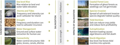
The coastal aquifer is an important resource for irrigation in agricultural areas. However, both aquifers and coastal agriculture/farmlands are vulnerable to seawater intrusion, which can result in substantial adverse consequences for the aquifer and crop production. Seawater intrusion is the landward movement of saline water into freshwater aquifers arising due to natural conditions, climate variability, and/or human activities (Ivkovic et al. Citation2012). Movement of saline water intensifies during surface water consumption and contamination, excessive groundwater pumping, and withdrawals from coastal wells which influences the coastal agricultural areas and low-salt tolerant crops negatively, including changes in soil salinity, reduction in water availability, and decrease in crop yield (Duan Citation2016). Intrusion is also driven by an increase in sea level, rainfall shortages, and occurrence of storm surges leading to coastal inundation, and an increase of salt concentration in brackish water which can augment the effects of drought. Tully et al. discussed the five main drivers of seawater intrusion: (1) sea-level position relative to land and water table; (2) frequency and magnitude of storms and tides; (3) frequency and duration of drought; (4) water use patterns; and (5) hydrologic connectivity. Each of the drivers varies spatially, temporally, and in terms of frequency and duration (). Consequently, salinization can occur gradually or rapidly, depending on the unique combination of drivers at a specific location (Citation2019, 6:368–378).
Figure 1. Drivers of seawater intrusion and their impacts (Weissman, Tully, and McClure Citation2020; adapted from Tully et al. Citation2019, 6:368–378).
Irrigated agriculture accounts for 70% of worldwide freshwater use and withdrawal (Dar Citation2017; Duan Citation2016). Agriculture serves as the main livelihood and driving force of the Philippines’ economy, with most coastal communities depending on crop production (Aklan Provincial Government Citation2019). Regarding water usage, a high percentage is allocated to agricultural purposes. As of 2009, freshwater has become the primary source of water withdrawal, accounting for the highest proportion of global consumption (Frenken Citation2012). Furthermore, the rates and demands for freshwater continue to rise (Dar Citation2017; Duan Citation2016). In addition to freshwater demands, various climatic factors influence water salinity. These demands and climatic factors render coastal agriculture vulnerable to soil and water salinity, leading to direct and indirect impacts on agricultural production (Alam et al. Citation2017). Different crops have varying salinity thresholds or tolerances, and if crops with low salt tolerance are exposed to saline water, agricultural production will be highly affected. The constant intrusion of seawater also leads to the accumulation of salts in the soil, causing damage to land productivity and resulting in economic losses (Burger and Čelková Citation2003, 7:314–320; Dar Citation2017; Duan Citation2016; Nguyen Citation2016). Conducting a vulnerability assessment is significant to demonstrate the current and potential future vulnerability of coastal agriculture to seawater intrusion.
The Municipality of Kalibo (Province of Aklan, Philippines) has been selected as the study area (). Kalibo is located on the northeastern border of Aklan and is bounded on the northeast by the Sibuyan Sea. Kalibo’s terrain is generally flat, with slope ranging from 0% to 3%, and favors both agricultural and urbanization growth. Land is mostly devoted to agriculture (62.2% of the total land area) and is planted with root crops, fiber crops, rice, coconuts, and other high value crops. Kalibo is situated in a Type III climate zone, which is characterized by a relatively dry period from November to April and a wet season for the rest of the year (FAO Citation2019). Agriculture, with rice as the primary crop, is the main source of livelihood in Aklan and Kalibo. In addition to rice, other high-value crops such as coconut, banana, mango, rambutan, and lanzones are also grown, contributing to the local economy (Aklan Provincial Government Citation2019). The land cover map indicates that rice is the most widely cultivated crop in Kalibo. The rice harvesting season was considered when selecting images, as it lasts for approximately 30 days from mid-September to October, within a 190-day cycle (Arnold Citation2004).
Figure 2. Study area in Kalibo with political boundaries and LiDAR-derived agricultural land cover map.
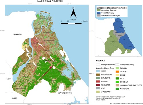
Kalibo has a total of 16 barangays, 7 of which are coastal barangays/farmlands or those barangays with agricultural lands near the shore or located in the coastal areas. While all barangays are considered, the assessment primarily focuses on the coastal barangays, namely, Bachaw Norte, Buswang Old, Caano, and Mabilo. These coastal agricultural barangays were selected by local officials and agricultural experts with firsthand experience on seawater intrusion. These areas are typically low-lying, making them susceptible to seawater intrusion.
The excessive pumping of groundwater from wells can lead to a decline and depletion of the water table resulting in the seawater to move inland and upward (The Groundwater Foundation Citation2022; USGS Citation2018). JICA (Citation2012) highlighted the negative impacts of seawater intrusion on agricultural production, particularly on rice. To address these issues, different measures for mitigation including the development of irrigation systems, promotion of salt-tolerant crop species, and proper management of water resources have been recommended. However, these measures can be implemented effectively if the vulnerability of coastal agriculture to seawater intrusion is properly addressed, assessed, and understood.
Following the Intergovernmental Panel on Climate Change (IPCC) framework, this study assessed vulnerability in terms of the system’s degree of exposure to hazards, sensitivity to climate variability, and its adaptive capacity to environmental changes relevant to seawater intrusion (Citation2017). Vulnerability is driven by the levels of exposure, sensitivity, and adaptive capacity. Systems with high exposure and/or sensitivity and lower adaptive capacity are more vulnerable. On the contrary, a system is less vulnerable when exposure and/or sensitivity is low and adaptive capacity is high. Therefore, to mitigate vulnerability, it is necessary to reduce the impact and/or increase adaptive capacity (Koh Citation2011, 411–427).
The assessment and developed models aimed at enhancing knowledge and increasing awareness of decision-makers, local and national stakeholders to seawater intrusion vulnerability for better planning and management. They will also serve as a guide in enhancing the community’s understanding of the indicators of seawater intrusion. The results are expected to provide information to farmers and local government units regarding the impacts of seawater intrusion on their farmlands.
2. Materials and methods
The vulnerability assessment of coastal agriculture to seawater intrusion considered the combined environmental, social, physical, and ecological contexts encompassed by climatic variations, and how they interact with each other (Bogardi, Birkmann, and De Léon Citation2005). The extent of assessment and/or unit of analysis is based on the 500 × 500-meter grid following the IPCC framework of vulnerability assessment (IPCC Citation2014, Citation2017).
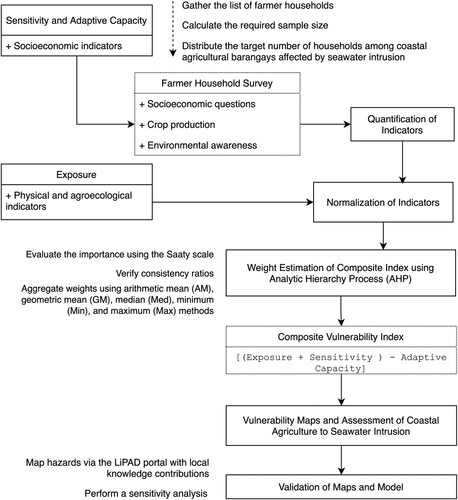
The analysis of vulnerability factors considered the availability of relevant datasets. Exposure indicators included the agricultural land use/cover map, distance to shoreline, rate of sea-level rise, elevation of land area, vegetation and salinity indices, extraction rate and levels, and hydraulic property. Sensitivity and adaptive capacity indicators were administered to farmer household surveys. Weights for each indicator were determined using the Analytic Hierarchy Process (AHP) and were combined using different aggregation methods. Results were integrated to collectively assess the vulnerability. Maps were validated through local’s knowledge of hazard existence and the assessment of the model was tested through the sensitivity analysis following the one-at-a-time (OAT) method (). Reference materials and relevant indicator datasets were utilized and served as inputs for the vulnerability component indices.
Figure 3. Methodological framework for assessing vulnerability of coastal agriculture to seawater intrusion.
2.1. Vulnerability indicators
Indicator-based assessment was conducted in the coastal barangays in Kalibo. Indicators of exposure, sensitivity, and adaptive capacity relevant to seawater intrusion have been selected and validated through participatory methods such as focus group discussions (FGD) and key informant interviews (KII). Indicators included the physical, agroecological, and socioeconomic parameters. The selection considered the following: each indicator must be agriculture-specific or related; indicator has predictive value to the assessment; availability and accessibility of the data; and the type of data, preferably, ordinal, interval, or ratio types.
The exposure index assesses the extent or degree to which coastal agriculture is vulnerable to seawater intrusion. The physical and agroecological indicators were considered in the exposure component and were estimated from models developed in this study (). Various sources of information, including data gathered from national and local offices, reports, expert opinions, field surveys, or a combination of these sources, were utilized.
Table 1. List of exposure indicators, concept, and importance in assessing vulnerability.
When assessing the vulnerability of coastal agriculture to seawater intrusion, it is important to consider both surface and subsurface factors. Surface analysis includes data on land cover, elevation, and groundwater extraction rates. Subsurface analysis includes indicators such as hydraulic conductivity and groundwater levels. However, some of the subsurface data were either outdated or unavailable and may have limited utility in assessing the vulnerability of groundwater and aquifers to seawater intrusion. Thus, the study primarily focused on assessing soil and crop vulnerability rather than subsurface factors.
Sensitivity captures characteristics of farmer households and crops that are influenced by the vulnerability associated with seawater intrusion. The assessment considers various sensitivity indicators (). On the other hand, adaptive capacity refers to the ability of agricultural lands to adapt with seawater intrusion. It reflects the resilience and adaptability of farmer households in responding to, coping with, and recovering from the impacts of hazards (Weis et al. Citation2016, 136:615–629). Indicators of adaptive capacity vary and include factors such as income from non-agricultural activities, savings, access to technology and information, economic capability, institutional capability, availability of disaster and hazard policies, and crop selection (). The evaluation of socioeconomic indicators was conducted through household surveys, which included the assessments of crop production and environmental awareness.
Table 2. List of sensitivity indicators, concept, and importance in assessing vulnerability.
Table 3. List of adaptive capacity indicators, concept, and importance in assessing vulnerability.
2.2. Data collection and analysis
2.2.1. Collection of socioeconomic data from farmer household surveys
The collection of socioeconomic data from household surveys was carried out using a random sampling strategy. Socioeconomic data was analyzed and used as inputs in determining the coastal agriculture’s sensitivity and adaptive capacity to the impacts of seawater intrusion. Assessments for these components were limited on the surveyed farmer household data and had greater reliance on expert judgement in comparison with the exposure assessment.
The respondents were households engaged in agricultural activities, excluding those involved in poultry and livestock. A 99% confidence interval and a 10% margin of error were used to determine the household sampling size, with the distribution of the target households based on an 80% response rate. However, the initial household survey did not yield enough respondents due to low awareness of seawater intrusion and some respondents declining to participate as their farmlands were not yet affected. As a result, the survey was revised to focus on barangays that have experienced or are currently experiencing seawater intrusion in their farmlands. These are the coastal barangays that have been verified by the local chairpersons or barangay captains with seawater intrusion experience. Out of the 136 targeted households, only 75 (55%) participated and provided socioeconomic data that is necessary for assessing sensitivity and adaptive capacity indicators.
2.2.2. Agricultural land use and analysis of the physical and geographical indicators
The information on the relevant land use and cover types in Kalibo was derived from the agricultural land cover map generated from the classification of Light Detection and Ranging (LiDAR) data using object-based image analysis (OBIA). Information on the extent and location of agriculture land use in the coastal zone is important in identifying agricultural lands closer to the coast as these areas may be more vulnerable to the effects of seawater intrusion, such as soil salinization which can have an impact on crop production (USDA Climate Hubs Citation2019; Weissman, Tully, and McClure Citation2020). A geographical parameter, the distance to shoreline indicator, was used in assessing the distance of farmlands from the coast, or the proximity of agricultural land to coastline. In this study, distance was estimated using coastal vignettes, which refers to the cartographic representations of the water-land boundary providing a visual representation of the distance between the coast and the agricultural land (Gopalakrishnan et al. Citation2019; Miller Citation2012).
The land cover map was updated to reflect land use, with non-agricultural classes excluded and the remaining classes were reclassified into three categories: trees, grain crops, and oil crops. The extent of agricultural land use within each grid and barangay boundary was then calculated to determine the total land use value within each grid (measuring 500 × 500 meters). The extent of each grid with agricultural area was also computed, and the results of the two calculations were used to determine the percent grid coverage of land use value to land use area.
Higher rates of sea-level rise leading to frequent and severe flooding can increase the risk of seawater intrusion into coastal farmlands. To assess the impact of rising sea-levels on farmlands, two raster datasets were created: one representing seawater, and the other showing the potential area of inundation. The seawater raster was generated by identifying areas that are at or below sea level, while the potential area of inundation was produced by identifying raster values that are at or below 2 meters, which is the highest recorded tide in 2019 for Kalibo based on tide times and tide charts (Tideschart Citation2019). To estimate the 2-meter inundation scenario, the sea-level raster was subtracted from the raster with elevations below or at 2 meters.
Assessing the elevation of agricultural areas is critical in determining their vulnerability to seawater intrusion and flooding caused by sea-level rise. It is also essential to consider the impact on its drainage patterns and the direction of groundwater flow. An area of low elevation will have a water table that is closer to the surface, making it more susceptible to seawater intrusion (Bhattachan et al. Citation2018; Hajji et al. Citation2022; USDA Climate Hubs Citation2019; Weissman, Tully, and McClure Citation2020). To quantify the sensitivity of an area based on its elevation, the elevation data (above mean sea level) was reclassified into five sensitivity classes, each represented by a numerical value: ‘5’ for very highly sensitive class (elevation <0.5 meters), ‘4’ for highly sensitive class (elevation between 0.5 and 1.5 meters), ‘3’ for medium sensitive class (elevation between 1.5 and meters), ‘2’ for low sensitive class (elevation between 2.5 and meters), and ‘1’ for very low sensitive class (elevation >3.5 meters). The value of the elevation indicator was calculated by multiplying the reclassified value (representing the sensitivity class) by the elevation grid area. To produce this indicator, the data was processed by excluding non-agricultural areas and reclassifying the remaining elevation values into the corresponding sensitivity classes.
2.2.3. Processing of vegetation and soil salinity indicators
Vegetation was used as an indirect indicator to predict and map soil salinity and with high consideration of vegetation salinity. Sentinel-2A images were used in the estimation. Salinity index highlights the surface reflectance of salt-affected regions and vegetation index highlights vegetated areas. Salinity and vegetation indices can help track salinity changes in vegetated areas (Azabdaftari and Sunar Citation2016; Elhag Citation2016; Taghadosi, Hasanlou, and Eftekhari Citation2019, 52:138–154). The Normalized Difference Vegetation Index (NDVI) value can be used to characterize the growth of rain-fed rice (Suwannachatkul et al. Citation2019). The downloaded and converted Sentinel-2A images were transformed into NDVI using EquationEquation (1)(1)
(1) :
(1)
(1) where
stands for the near-infrared band and
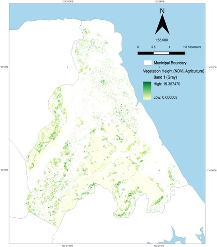
for the red band. NDVI maps from August 2017 to December 2018 were analyzed to determine which image date best represents the pre-harvest season of rice in Kalibo. The expected NDVI values for the target state and percent cloud coverage were taken into consideration during this analysis. During the pre-harvest season, rice growth becomes dry, resulting in a drop in the NDVI value. It was also observed that the harvest season typically occurs in mid-September to October.
The analysis of image data revealed that September 2017 and February 2018 had the highest majority of NDVI values (0.75). However, the maximum value (0.99487) was observed in November 2017. Non-agricultural areas were masked out using a LiDAR-derived map and pixel values from 0.02 to 0.20 to ensure accurate NDVI values. The September images, which best represented the target state, were used in the vegetation index. This was further validated by focusing solely on the rice land cover ().
Figure 4. The NDVI map for September 2018, focusing on rice land cover to emphasize the pre-harvest season. This map is utilized as an input for the vegetation index indicator. The index maps are generated from NDVI subsets, LiDAR-derived agricultural land cover, and a false color composite image.
In addition to the vegetation index, several salinity indices derived from Sentinel-2A were considered to detect and predict salinity in areas with high vegetation cover. These indices are shown in .
Table 4. Indices derived from Sentinel-2A that were utilized in the estimation of vegetation salinity.
The Salinity Index (SI) is a measure of salinity that combines the blue and red bands and is sensitive to the surface reflectance of salt-affected areas with sparse vegetation cover (Douaoui, Nicolas, and Walter Citation2006, 134:217–230; Elhag Citation2016). Another combination for SI is the red and near-infrared bands, which is affected by salt crust, soil color and moisture content. Saline soils with a smooth and light salty crust surface exhibit high reflectance, while those with a coarse, dark, puffy surface show low reflectance (Asfaw, Suryabhagavan, and Argaw Citation2018, 17:250–258). The Salinity Ratio (SR) is computed using the ratio between the red and near-infrared bands and the green and near-infrared bands. The use of near-infrared bands can be highly correlated with field electrical conductivity, resulting in accurate estimations for satellite-based salinity detection. The blue and green bands are also used in this index, which can show an increase in the reflectance when salinity is present (Morshed, Islam, and Jamil Citation2016). However, cross-checking with the field data was not performed in this study.
Vegetation Soil Salinity Index (VSSI) is an index used to distinguish between soil and vegetation stress. Canopy Response Salinity Index (CRSI) is used to determine the salinity of the root zone. While CRSI is not a vegetation index specifically designed for salinity, it can be compared with other vegetation indices to provide better estimates of salinity levels. CRSI is used to estimate salinity based on canopy reflectance, where reflectance increases in the blue, green, and red ranges of the electromagnetic spectrum and decreases in the near-infrared range when the crop is stressed by root zone salinity, as noted by Scudiero et al. (Citation2017, 71:231–238).
The Normalized Difference Wet Index (NDWI) is a useful indicator for plant water stress that is highly correlated with plant water content. It is derived from the near-infrared and short-wave infrared channels and is effective in enhancing the reflectance spectra of wet soil (JRC-European Commission Citation2011; Gao Citation1996, 58:257–266). High NDWI values indicate a high vegetation water content and a high fraction of vegetation canopy, while low NDWI values indicate a low vegetation water content and a low fraction of vegetation canopy. During periods of water stress, NDWI typically decreases due to a decrease in the amount of water in vegetation canopies, which is related to the soil water content (JRC-European Commission Citation2011). Unlike the NDVI, NDWI is less sensitive to atmospheric scattering effects (Noeda Citation2012), however, it does have a limitation: NDWI tends to overestimate water bodies due to its sensitivity to built-up structures (Sentinel Hub Citation2017).
The Combination Salinity Index (CSI) was generated by combining multiple salinity indices, including SI, SR, VSSI, CRSI and NDWI. Notably, NDVI was excluded from the index because CRSI, already integrated, prove more effective in detecting salinity than NDVI (Dehni and Lounis Citation2012, 33:188–198). The CSI is mapped based on the extent of the LiDAR-derived agricultural land cover map. This approach also incorporates information about built-up and water classes, addressing the overestimation of water bodies from NDWI.
To further complement the analysis, a crop height map was generated and combined with the NDVI map to distinguish trees based on their height levels and differentiate agricultural crops from other types of vegetation and other surface features in the study area of Kalibo (). Additionally, the trend of salinity with respect to distance from the coast was examined. For this purpose, 21 zones were created with a 300-meter distance interval.
Figure 5. Approximation of agricultural crop height.
2.2.4. Estimation of groundwater and hydraulic property indicators
The groundwater extraction rate refers to the amount of groundwater withdrawn from an aquifer or well for human and agricultural use (Bierkens and Wada Citation2019; USGS Citation2018). To measure the quantity of water extracted in a particular area, the average monthly discharge diverted from the Aklan river irrigation system was used as an indicator. This is an important indicator to consider, as high rates of groundwater extraction, such as excessive pumping of wells, can lead to a decline in the water table and increase the likelihood of seawater seeping into the groundwater aquifers (Reilly et al. Citation2008; USGS Citation2019).
The groundwater levels indicator, which refers to the depth at which groundwater is found below the land surface, was estimated from JICA’s report in 2012, which recorded groundwater data levels in Kalibo. As seawater intrusion occurs, saltwater moves into the aquifer, displacing the freshwater and causing the groundwater levels to decline (Alfarrah and Walraevens Citation2018; Barlow Citation2003). The averages of the rainy season and dry season groundwater levels were interpolated to grid values, along with the locations of wells.
The hydraulic conductivity (K-value), a measure of a material’s ability to transmit water, is estimated using a model that considers soil type and permeability, with data sourced from the Department of Environment and Natural Resources – Mines and Geosciences Bureau (DENR-MGB) and the Philippine Rice Research Institute (PhilRice). The model, based on Arras (Citation2014), estimates K-value using factors such as topography, flow path distance, recharge, and aquifer thickness. The study assumes a steady-state dynamic equilibrium, an unconfined aquifer, and groundwater flow following Darcy’s Law. The K-value is then calculated using EquationEquation 2(2)
(2) , where, K represents the hydraulic conductivity (length/time), W is the length of effective groundwater drainage (length), R is the recharge rate (length/time), d is the valley depth from channel water level (length), and H is the aquifer thickness (length).
(2)
(2) The results are summarized in . Note that this study focuses on the impact of salinity on crops and soil, not groundwater.
Table 5. Summary of estimated K-values based on various approaches.
2.3. Quantification and normalization of indicators
The indicator parameters were measured both quantitatively and qualitatively. To enable comparison of indicators across barangays on the same scale, linear normalization was applied to the quantified indicator values (OECD Citation2008). Equation Equation(3)(3)
(3) was utilized for normalization of indicator values.
(3)
(3) where
stands for the normalized value of indicator
of the barangay/municipality
,
refers to the original value of the indicator
of the barangay/municipality
,
is the highest value among all the barangays/municipalities, and
is the lowest value among all the barangays/municipalities.
The collected household surveys for sensitivity and adaptive capacity were quantified and their values were also normalized, including the exposure indicators.
2.4. Weight estimation using AHP
The AHP weighting method, proposed by Saaty (Citation1980), was utilized to determine appropriate indicator weights while considering the 20% threshold consistency rate. The consistency check was calculated using Equation Equation(4)(4)
(4) :
(4)
(4) where
refers to the maximum allowable
at the 20% threshold, and
represents the number of indicators. Experts were requested to rate the level of importance of the indicators using Saaty’s rating scale, which includes a graduated system of numbers describing the intensity of importance ().
Table 6. The Saaty rating scale.
The relative importance for each indicator, including the rating of land cover classes, was determined by consulting 17 experts from national agencies, organization, academia, and local offices in Aklan, Kalibo and respective barangays using survey questionnaires. Only responses with consistency ratios within the 20% threshold were considered in the calculation of AHP, with a total of 4 responses for exposure, 4 for sensitivity, 6 for adaptive capacity, and 10 for land use/cover classes (). The consulted experts for AHP weights were categorized into five groups: (1) barangay experts, including heads from barangay offices (i.e. chairman, agriculture committee, agriculture technician, secretary); (2) city experts, including officers from offices in agriculture, planning and development, and disaster risk reduction management; (3) provincial experts from offices in agriculture and environment and natural resource; (4) experts from national agencies; and (5) experts from academia.
Table 7. Number of responses from experts and stakeholders.
Weights were used to calculate the values for the exposure, sensitivity, and adaptive capacity indices. Different aggregation methods such as arithmetic mean, geometric mean, median, minimum, and maximum were employed to combine the individually calculated weights. These methods were used to identify any potential gaps in the complex individual information and to evaluate whether the combination of weights using different approaches would affect the output maps.
2.5. Composite vulnerability index assessment
Models were developed to assess the level of salinity in coastal farmlands. The assessment considered the analysis of multidimensional complex systems to easily comprehend the results as a range of values and rankings to aid planners, decision-makers, and stakeholders (USAID Citation2014). A composite index was created by integrating the indicators of exposure, sensitivity, and adaptive capacity to calculate vulnerability using Equation Equation(5)(5)
(5) :
(5)
(5) The vulnerability assessment of coastal farmlands in Kalibo included the generation of maps, using weights determined through AHP and aggregated using various methods. Maps and values were produced for each vulnerability indicator, and vulnerability estimates were derived based on the vulnerability values and the rating scheme outlined in .
Table 8. Vulnerability values and ratings.
The K-indicator, which introduced some uncertainty, generated multiple outputs, resulting in different versions of vulnerability assessments. K-values were estimated using: (1) a developed model, (2) soil type, (3) soil permeability, and (4) the average of the three K-values.
A total of 20 exposure maps, 5 sensitivity maps, 5 adaptive capacity maps, and 20 vulnerability maps were generated. The assessment of agricultural vulnerability to seawater intrusion covered all barangays, with a particular focus on Bachaw Norte, Buswang Old, Caano, and Mabilo. It is important to note that the exposure maps were able to assess both agricultural and non-agricultural coastal barangays.
2.6. Validation of maps and models
The vulnerability maps generated were compared with geotagged areas of seawater intrusion available on the LiDAR Portal for Archiving and Distribution (LIPAD) website. These geotagged areas were identified based on the expertise of city agricultural professionals who have knowledge of seawater intrusion occurrences over the past 5–10 years.
To assess the uncertainties and reliability of the models, sensitivity analysis was conducted using the OAT method. This approach evaluates how changes in individual input variables or indicators impact the model’s output. It assesses the robustness and extent of output variation when parameters are changed (Al-Mashreki et al. Citation2011, 9:1102–1111). Specifically, it helps identify which input variables or indicators have the most significant influence on the model’s results and assesses the model’s reliability (Kaplan Financial Limited Citation2020).
The behavior of the model and the impact of parameter changes were explored by varying weights assigned to exposure indicators. Eighteen different weighting schemes for each exposure indicator were used, resulting in 162 iterations with +/ – 10% variations. Throughout this process, the weights of other indicators were kept unchanged.
The sensitivity analysis primarily focused on exposure indicator values. The values were derived from the average of three K-values obtained using the arithmetic mean aggregation method. By applying ±10% weight variations to indicators such as land use/cover map, distance to shoreline, rate of sea-level rise, elevation of land area, vegetation index, soil salinity, groundwater extraction rate, groundwater levels, and hydraulic property, the study aimed to assess the model’s sensitivity.
3. Results and discussion
3.1. Characteristics of surveyed farmer households
Household characteristics show that most household participants are not members of any farmer or agriculture-related organization. Most farmer households own at least one tube well. 65.3% of household respondents indicated that their overall income comes from both agriculture and non-agriculture sources, but only 16% have attended trainings related to agriculture. Also, 64% of the households have their own tube wells and 54.7% have domestic water treatment ().
Table 9. Characteristics of participating household respondents from Bachaw Norte, Buswang Old, Caano and Mabilo.
3.2. Relative importance of vulnerability indicators
Agricultural land use and vulnerability indicator weights are presented in and , respectively. In the case of land use, the arithmetic mean aggregation method was employed to combine the weights. Grain crops, such as rice and corn, received higher weights compared to oil and tree crops, which were assigned lesser weights. For vulnerability indicators, the weights were aggregated using various methods including arithmetic mean, geometric mean, median, minimum, and maximum. The resulting values indicate minimal differences, as the rankings provided by experts during the consultation process remained consistent.
Table 10. Weights of agricultural land use calculated from AHP and arithmetic mean aggregation method.
Table 11. Vulnerability indicators and corresponding weights determined using AHP and aggregation methods.
3.3. Satellite-based estimation of salinity
Grain crop areas exhibit varying levels of salinity, ranging from medium to high (). The extent and severity of salinity depend on both the crop type and its height. Inland zones, located 3600–5700 meters away from the coast, tend to have higher salinity values. This is likely due to the factors such as soil composition (Shahid, Zaman, and Heng Citation2018, 43–53), irrigation practices (Nick et al. Citation2024, 38:17), and historical salt accumulation (Shahid, Zaman, and Heng Citation2018, 43–53). In contrast, coastal areas experience a gradually decrease in salinity values. The proximity to the coast allows for leaching – the process by which excess salts are washed away by rainfall or irrigation. Coastal soils benefit from this natural leaching mechanism, resulting in lower salinity levels (Andros Citation2021).
Figure 6. Combination salinity index excluding non-agricultural areas shown as green areas in this map.
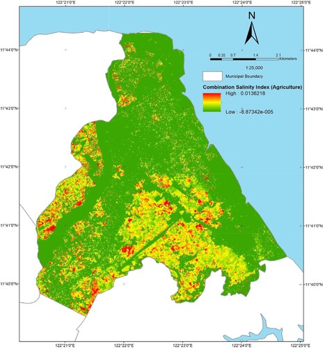
Furthermore, there exists a decreasing trend in salinity as crop height increases. The reduced salinity can be attributed to several factors such as root behavior (both root depth and soil surface layer) and increased transpiration in taller crops (Shelden and Munns Citation2023). However, beyond a certain height (specifically 18 meters), salinity abruptly increases – this may be influenced by factors such as root architecture and nutrient uptake.
3.4. Vulnerability assessment of coastal barangays
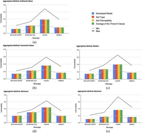
The vulnerability assessment of the coastal barangays was conducted using different aggregation methods (arithmetic mean, geometric mean, median, minimum, and maximum) and approaches to estimate K-values (based on a developed model, soil type, soil permeability, and an average of the three K-values). The computed vulnerability values for these selected coastal barangays are as follows:
Bachaw Norte: The vulnerability ranges from low to moderately low (≥ 0 to ≤ 0.4) across all approaches and aggregation methods.
Buswang Old: The vulnerability is moderately low (> 0.2 to ≤ 0.4) for all approaches in median and minimum aggregation methods, and ranges from low to moderately low for all approaches in arithmetic mean, geometric mean, and maximum.
Caano: The vulnerability ranges from moderately low to moderately high (> 0.2 to ≤ 0.8) for all aggregation methods, except in geometric mean, which has a rating of moderately low to moderate (> 0.2 to ≤ 0.6).
Mabilo: The vulnerability ranges from low to moderately low for all approaches used in the arithmetic mean, geometric mean, median, and minimum aggregation methods, and from low to moderate (≥ 0 to ≤ 0.6) for the maximum in all approaches, except for the results derived from the developed model.
The assessment indicated that Caano has a relatively higher vulnerability compared to other selected coastal barangays. The computed vulnerability values of coastal agriculture/farmlands, in terms of aggregation methods and different approaches used in estimating K-values, are illustrated in .
Figure 7. Vulnerabilities for coastal agriculture/farmlands in terms of aggregation methods ((a) arithmetic mean (b), geometric mean (c), median (d), minimum (e), maximum) and different approaches used in estimating K-values. Note that the vulnerability levels are similar across the different K-value estimation approaches.
Each of the selected barangays exhibited unique characteristics contributing to their respective vulnerability levels ( and ). Bachaw Norte, despite its proximity to a river, exhibited the least vulnerability among the barangays, with levels ranging from low to moderately low. The vulnerability assessment focused on the distance of crops from the sea, not the river. Despite the area’s low adaptive capacity, its reduced vulnerability can be attributed to its low exposure and sensitivity. Various indicators, from land use to groundwater exposure, were considered in the assessment. The map predominantly shows low values, with the hydraulic property indicator being an exception.
Figure 8. Maps of coastal agriculture vulnerability in the barangays of Kalibo, Aklan, Philippines using various aggregation methods and K-value estimation techniques, including a developed model, soil type, and soil permeability: (a) arithmetic mean (b), geometric mean (c), median (d), minimum (e), maximum.
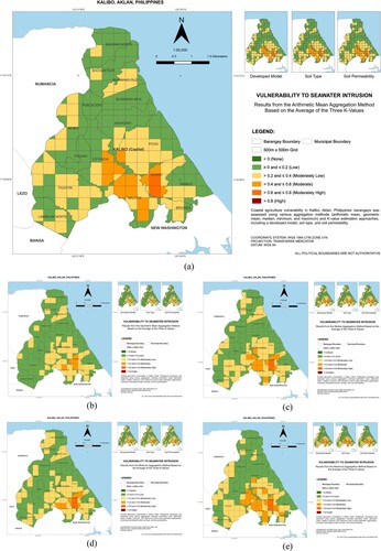
Figure 9. Components of vulnerability to seawater intrusion using various aggregation methods and K-value estimation techniques, including a developed model, soil type, and soil permeability: (a) arithmetic mean (b), geometric mean (c), median (d), minimum (e), maximum.
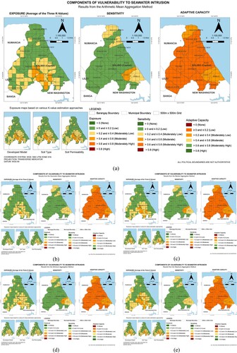
Buswang Old, located near a river and comprising significant fishpond areas, exhibited vulnerability ratings from low to moderately low. These ratings vary based on the aggregation method used, with notable differences between the minimum and maximum methods. The area’s land cover is predominantly oil crops. Despite lower impacts and adaptive capacity, there is potential for high vulnerability values under certain aggregation methods.
Caano, with its coastal fishponds and agricultural lands, was identified as the most vulnerable area. Vulnerability ratings range from moderately low to moderately high, except when using the geometric mean method, which shows moderate vulnerabilities. The exposure map reveals an increasing trend inland, with vulnerability ratings from low to moderate. The sensitivity map shows moderate ratings, while the adaptive capacity map indicates moderately low ratings. High exposure indicator values are observed for factors like sea-level rise, vegetation and salinity indices, hydraulic property, shoreline distance, and rice areas.
Mabilo's vulnerability ratings ranged from low to moderate, with variations based on the aggregation method used. The land cover includes coastal residential areas, rice crops, and large fishponds, with the latter two showing higher vulnerability. The hydraulic property indicator shows a moderate rating, while sensitivity and adaptive capacity are moderately low. Differences in vulnerability maps are observed between the minimum and maximum aggregation methods, especially in the exposure indicators.
3.5. Relationships between the potential impact and adaptive capacity
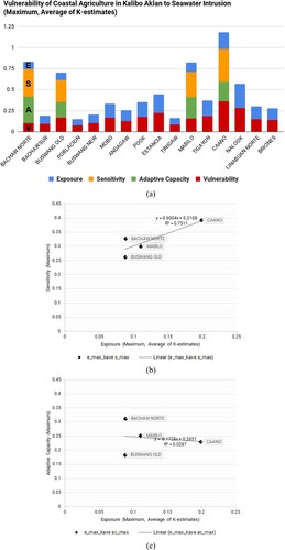
The computed vulnerability values and scatter plots of exposure, sensitivity, and adaptive capacity values of coastal barangays, based on the average of the three K-values, illustrate the relationship between the potential impact, determined by exposure and sensitivity components caused by seawater intrusion, and the adaptive capacity (). Vulnerability is a function of exposure, sensitivity, and adaptive capacity, and a low adaptive capacity relative to exposure and sensitivity contributes to high vulnerability. On the contrary, higher adaptive capacity helps reduce the effects of exposure and sensitivity, resulting in low vulnerability (Thomas et al. Citation2019). The plots of exposure versus sensitivity are expected to have a steep inverse slope, while exposure versus adaptive capacity should have a steep slope to counteract the effect of exposure and achieve low vulnerability ratings, i.e. high exposure and low sensitivity, and low exposure and high adaptive capacity.
Figure 10. Vulnerability assessment of agricultural barangays in Kalibo, Aklan to seawater intrusion: (a) computed vulnerability values using the results from the arithmetic mean aggregation method based on the average of the three K-values, (b) scatter plot showing the relationship between exposure and sensitivity values, and (c) scatter plot illustrating the relationship between exposure and adaptive capacity values.
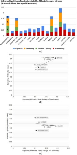
Figure 11. Vulnerability assessment of agricultural barangays in Kalibo, Aklan to seawater intrusion: (a) computed vulnerability values using the results from the geometric mean aggregation method based on the average of the three K-values, (b) scatter plot showing the relationship between exposure and sensitivity values, and (c) scatter plot illustrating the relationship between exposure and adaptive capacity values.
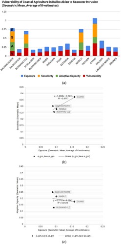
Figure 12. Vulnerability assessment of agricultural barangays in Kalibo, Aklan to seawater intrusion: (a) computed vulnerability values using the results from the median aggregation method based on the average of the three K-values, (b) scatter plot showing the relationship between exposure and sensitivity values, and (c) scatter plot illustrating the relationship between exposure and adaptive capacity values.
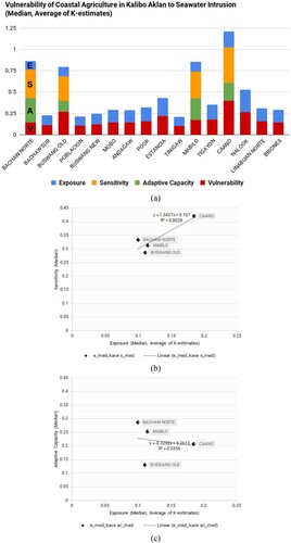
Figure 13. Vulnerability assessment of agricultural barangays in Kalibo, Aklan to seawater intrusion: (a) computed vulnerability values using the results from the minimum aggregation method based on the average of the three K-values, (b) scatter plot showing the relationship between exposure and sensitivity values, and (c) scatter plot illustrating the relationship between exposure and adaptive capacity values.
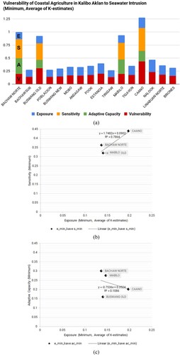
Figure 14. Vulnerability assessment of agricultural barangays in Kalibo, Aklan to seawater intrusion: (a) computed vulnerability values using the results from the maximum aggregation method based on the average of the three K-values, (b) scatter plot showing the relationship between exposure and sensitivity values, and (c) scatter plot illustrating the relationship between exposure and adaptive capacity values.
The results from the arithmetic mean based on the average of K-values show Caano as the most vulnerable with a rating of 0.3811 followed by Buswang Old with 0.2104, Mabilo with 0.1598, and Bachaw Norte with 0.1194 ((a)). Caano was observed to be the most exposed, with the highest sensitivity and low adaptive capacity. On the contrary, Bachaw Norte exhibited the highest adaptive capacity and is tagged as the least vulnerable, least exposed and has low sensitivity compared to the other coastal barangays ((b,c)).
Analyzing the results from other aggregation methods based on the average of K-values revealed that Caano was the most vulnerable, with ratings of 0.3571, 0.3976, 0.4357, and 0.3615 in geometric mean, median, minimum, and maximum respectively ((a)). Relationships among the three components (exposure, sensitivity, and adaptive capacity) also demonstrated high vulnerability, as high exposure, high sensitivity, and low adaptive capacity were observed ().
Based on the results shown in , the relationships among the three components indicated that the coastal barangays in Kalibo are vulnerable to seawater intrusion. Coastal agricultural barangays with high exposure also exhibited high sensitivity and low adaptive capacity. The vulnerability assessment results are likely influenced by various factors such as access to resources, type of governance, culture, and knowledge of local and international communities/agencies (Thomas et al. Citation2019).
3.6. Assessment of maps through local’s knowledge
Tagged areas with seawater intrusion included the following barangays: Bachaw Norte, Bachaw Sur, Buswang Old, Buswang New, Mabilo, Briones, and Nalook (). These areas are primarily located along the coast or at the mouth of the river. However, the assessment results show differences from the tagged areas, indicating that the assessment considered additional factors beyond just the proximity of farmlands to the ocean or the rising of water.
Figure 15. Areas identified by locals as experiencing seawater intrusion.
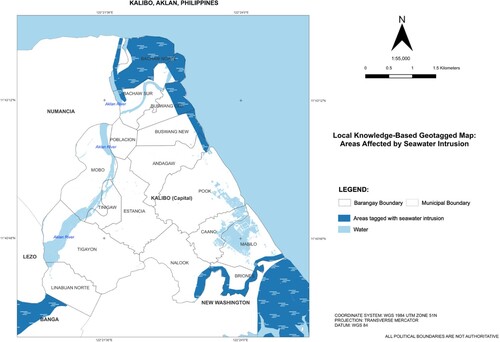
The selection of target barangays considered the knowledge and input of farmers and barangay officials. These stakeholders mentioned that seawater intrusion is affecting the productivity of farmlands in the barangays of Bachaw Norte, Buswang Old, Caano, and Mabilo. The intrusion is primarily caused by inundation resulting from rising water levels in both the ocean and river. The observed differences in the results can be attributed to the comprehensive nature of the assessment, which considered physical, agroecological, and socioeconomic indicators, rather than solely relying on distance or water level measurements. Furthermore, variations in estimations and observations among local farmers, officials, and agricultural experts were observed.
3.7. Assessment of model through sensitivity analysis
Sensitivity analysis results indicated the impact of modifying weights for different indicators on exposure values in the assessed barangays. When adjusting the weights for the land use/cover map indicator, there were decreased exposure values, with no significant differences observed in the coastal farmlands of Kalibo. Sensitivities were observed in all barangays when varying the weights for the distance to shoreline indicator, resulting in increased exposure in several barangays. Similar findings were observed for the rate of sea-level rise indicator, where increasing weights led to increased exposure in specific barangays.
The elevation of land area indicator showed decreasing exposure values in all barangays except for Poblacion. The vegetation index indicator resulted in decreased exposure values across all barangays, with slight changes observed in specific coastal farmlands. For the soil salinity indicator, increased exposure was observed in certain barangays, while the groundwater extraction rate indicator showed increased exposure in the +10% weight variations and decreased exposure in the -10% variations. The groundwater levels indicator exhibited decreasing exposure in all barangays, except for Linabuan Norte. Modifications in the weights for the hydraulic property indicator resulted in decreased exposure in all barangays, with specific variations observed in coastal farmlands. Overall, the sensitivity analysis provides insights into how variations in weighting schemes influence exposure values, highlighting the importance of each indicator in assessing coastal agriculture/barangays.
shows a summarized view of the exposure values obtained from the sensitivity analysis. It displays the changes caused by the application of ±10% weight variations to the exposure indicators. This figure provides a concise representation of the sensitivity analysis results, facilitating a quick assessment of the model's stability and robustness.
Figure 16. Summary of exposure values from sensitivity analysis using ±10% weight variations applied to land use/cover map (LULC), distance to shoreline (DTS), rate of sea-level rise (SLR), elevation of land area (ELEV), vegetation index (VI), soil salinity (SS), groundwater extraction rate (GER), groundwater levels (GL), and hydraulic property based on the average of the three K-values (K).
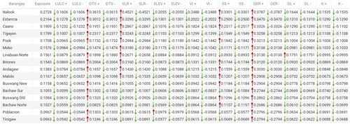
The sensitivity analysis of the models revealed that most indicators are sensitive to changing weight values. Through the OAT method, weights for each indicator were systematically modified, evaluating the resultant changes in exposure values. This analysis enables assessment of the sensitivity of the model to different weightings and highlights the relative importance of each indicator in determining the overall exposure assessment. Although the observed changes are minimal, they can still impact the resulting vulnerability assessment. It should also be noted that the implementation of the OAT method is relatively simple and does not account for assessing interactions between variables or the uncertainty of indicators, including potential model errors. It assumes that all other indicators remain constant, which is not realistic. Therefore, other sensitivity analysis methods, such as variance-based or regression-based methods, can be considered to account for interactions between variables (Business Case Preparation Citation2019; Kaplan Financial Limited Citation2020).
The assignment of weights applied in the vulnerability assessment is based on expert knowledge and awareness of the area, thus the generated maps and developed models can still be considered reliable. The results of the sensitivity analysis provide insights into how the assessment can be improved. Indicators with uncertainty and/or highly sensitivity should be weighted accordingly.
4. Conclusions and recommendations
This research assessed the vulnerability of coastal farmlands in Kalibo, Aklan, Philippines to seawater intrusion by considering exposure, sensitivity of resources, and adaptive capacity. The study utilized models and data from various sources, including agricultural maps, satellite imagery, and participatory methods such as interviews and surveys. The analysis included the development of salinity indices, estimation of vulnerability indicators, and generation of exposure, sensitivity, adaptive capacity, and vulnerability maps for selected barangays.
The assessment identified Caano as the most vulnerable barangay, while Bachaw Norte was identified as the least vulnerable. The exposure map highlighted Nalook, Estancia, and Caano as areas with the highest exposure levels to seawater intrusion. Sensitivity analysis provided insights for improving the assessment by testing different weighting schemes for indicators.
To facilitate the utilization of research outputs and relevant information, vulnerability maps were made publicly available through the PARMap Web Portal (https://parmap.dream.upd.edu.ph/) and the LiDAR Portal (https://lipad.dream.upd.edu.ph). This enabled local government units, stakeholders, and decision-makers to access the information and incorporate it into their decision-making process for developing programs and policies to reduce vulnerability and improve adaptability in coastal agriculture.
While the research utilized various indicators and available data, it acknowledged limitations due to the availability of surveyed farmer household data, records, and knowledge of locals and experts. To address these limitations, the study recommended expanding the selection of target areas by including farmlands near the coast and/or river. Additionally, socioeconomic data collection should consider recording the location of households to avoid generalizations in the assessment. In-depth and improved validation methods are also necessary, including intensive collection of groundwater data from wells and pumping stations, conducting pumping tests and georesistivity surveys in the field. It is crucial to consider geologic characteristics when estimating hydraulic conductivity, and detailed geologic maps should be acquired or requested from the relevant agency to enable a comprehensive assessment of subsurface, aquifer, and groundwater vulnerability, rather than focusing solely on soil and crop vulnerability.
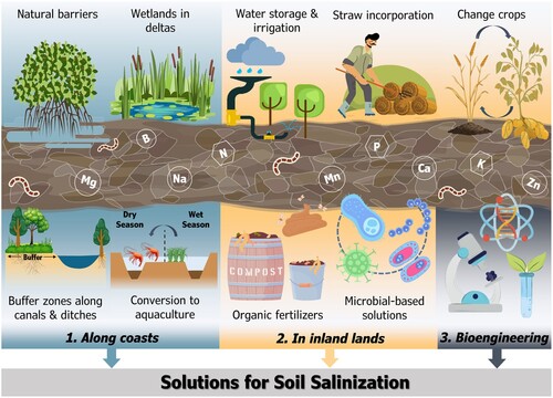
Salinity intrusion to coastal agriculture necessitates effective mitigation strategies; a sustainable response combining nature-based solutions (NBS) with bioengineering. Coastal areas benefit from NBS, which include restoring mangroves, wetlands, and natural buffers – these ecosystems act as barriers against seawater intrusion, maintaining soil quality and supporting agriculture. Inland areas can also adopt NBS through sustainable land use planning, afforestation, and managed aquifer recharge – these approaches help maintain freshwater lenses and reduce soil salinity. Bioengineering offers promise in selecting and creating crops adapted to saline conditions. Salt-tolerant crop varieties thrive in high-salinity soils, ensuring food security even in challenging environments. Research and development efforts should prioritize strengthening the resilience of staple crops (such as rice) against salinity stress. However, challenges and limitations must be considered: (1) implementing NBS requires collaboration among stakeholders, policy adjustments, and financial investments; (2) bioengineered crops must undergo rigorous testing to ensure safety, yield, and nutritional quality; and (3) balancing NBS with conventional approaches remains essential, especially in large-scale agricultural systems (Tarolli et al. Citation2024).
Tarolli et al. (Citation2024) suggest a synergistic approach: strategically planting salt-tolerant crops in NBS-implemented areas. This enhances soil health, increases yields, and improves livelihoods. This combined approach can support vulnerable regions worldwide, addressing hunger and climate change impacts. A conceptual framework () summarizes the mitigation solutions discussed. NBS and salt-tolerant crops offer hope for sustainable agriculture, safeguarding both food production and ecosystems.
Figure 17. A conceptual framework on sustainable solutions in mitigating soil salinization in agriculture (Source: Tarolli et al. Citation2024)
Overall, this research contributes to improving knowledge and awareness of seawater intrusion vulnerability in coastal agriculture and supports better planning and management approaches for decision-makers, stakeholders, and local communities. By addressing the limitations and incorporating further research recommendations, future assessments can enhance the accuracy and effectiveness of vulnerability assessments in coastal farmland.
Statements and declarations
Compliance with ethical standards
This paper adheres to all ethical standards and guidelines set forth by the relevant governing bodies.
Acknowledgements
The research presented in this manuscript was conducted as part of the R&D (Research and Development) initiatives at the University of the Philippines - Training Center for Applied Geodesy and Photogrammetry (UP-TCAGP). The project, PARMap (Agricultural Resources Extraction from LiDAR Surveys) under the Nationwide Detailed Resources Assessment Using LiDAR (Phil-LiDAR 2) Program, was funded by the Philippines’ Department of Science and Technology (DOST). The algorithms and workflows were developed utilizing the technical facilities and support provided by UP-TCAGP through the Phil-LiDAR 2 Program and PARMap Project. This support included the use of a detailed map of agricultural resources, including various crop types, derived from LiDAR and other remotely sensed data. The authors also acknowledge the Disaster Risk and Exposure Assessment for Mitigation (DREAM) Program and the Hazard Mapping of the Philippines using LiDAR (Phil-LiDAR 1) Program for the support in our research by allowing us to use the LIPAD website, which was instrumental in geotagging areas with seawater intrusion. The authors also recognized the Engineering Research and Development for Technology (ERDT) through the Faculty Research Dissemination Grant for sponsoring our publication charge. Reference materials and relevant indicator datasets were also gathered from various national agencies and government offices, including the: municipal boundary from the Philippine Statistics Authority (PSA), formerly known as the National Statistics Office (NSO); bathymetric LiDAR digital elevation model (DEM) and Interferometric Synthetic Aperture Radar (IFSAR) DEM from DREAM/Phil-LiDAR 1 Program; Sentinel-2 multispectral data; river discharge record of Aklan river irrigation system from 1977 to 2017 acquired from National Irrigation Administration (NIA) Region VI; groundwater data and well information from JICA and Local Water Utilities Administration (LWUA); and 2003 soil map from the Bureau of Soils and Water Management (BSWM). This manuscript acknowledges the researchers of the Phil-LiDAR 2 PARMap, consulted national and local experts, and the respondents for the farmer household surveys, all of whom have contributed to the attainment of the manuscript's objectives.
Disclosure statement
No potential conflict of interest was reported by the author(s).
Data availability
The maps and assessment results related to this study can be requested from the corresponding author. The data that supports the findings of this study are available on the PARMap Web Portal (https://parmap.dream.upd.edu.ph/). This portal serves as a repository for the knowledge products generated by the Phil-LiDAR 2 PARMap. Additionally, the LiDAR Portal (https://lipad.dream.upd.edu.ph/) provides primary access and distribution for the flood hazard and resource maps derived using LiDAR technology. For further inquiries, please direct your requests to the corresponding author.
Additional information
Funding
References
- Agriculture Improvement Act of 2018, 2, House of Representatives, 115th Congress. 2018. http://www.congress.gov/bill/115th-congress/house-bill/2/text.
- Aklan Provincial Government. 2019. Economy and Investment. Aklan Gov Ph. http://aklan.gov.ph/economy-and-investment/.
- Al-Mashreki, M. H., J. B. M. Akhir, S. A. Rahim, K. M. D. Lihan, and A. R. Haider. 2011. “GIS-Based Sensitivity Analysis of Multi-Criteria Weights for Land Suitability Evaluation of Sorghum Crop in the Ibb Governorate Republic of Yemen.” Journal of Basic and Applied Scientific Research 1 (9): 1102–1111. https://www.researchgate.net/publication/284675185_GIS-based_sensitivity_analysis_of_multi-criteria_weights_for_land_suitability_evaluation_of_sorghum_crop_in_the_Ibb_Governorate_Republic_of_Yemen.
- Alam, M. Z., L. Carpenter-Boggs, S. Mitra, M. M. Haque, J. Halsey, M. Rokonuzzaman, B. Saha, and M. Moniruzzaman. 2017. “Effect of Salinity Intrusion on Food Crops, Livestock, and Fish Species at Kalapara Coastal Belt in Bangladesh.” Journal of Food Quality 2017 (1): 1–23. https://doi.org/10.1155/2017/2045157.
- Alfarrah, N., and K. Walraevens. 2018. “Groundwater Overexploitation and Seawater Intrusion in Coastal Areas of Arid and Semi-Arid Regions.” Water 10 (2): 143. https://doi.org/10.3390/w10020143.
- Andros, M. 2021. Understanding Leaching and Soil Salinity. Semios. https://blog.semios.com/understanding-leaching-and-soil-salinity.
- Arnold, P. 2004. Season of Rice: The Process of Rice Farming. Patty Arnold. https://www.pattyarnold.com/process.html.
- Arras, T. L. 2014. A GIS Approach to Estimating Continuous Hydraulic Conductivity and Equivalent Hydraulic Conductivity. https://ir.library.oregonstate.edu/concern/graduate_thesis_or_dissertations/0v8385346.
- Asfaw, E., K. V. Suryabhagavan, and M. Argaw. 2018. “Soil Salinity Modeling and Mapping Using Remote Sensing and GIS: The Case of Wonji Sugar Cane Irrigation Farm, Ethiopia.” Journal of the Saudi Society of Agricultural Sciences 17 (3): 250–258. https://doi.org/10.1016/j.jssas.2016.05.003.
- Azabdaftari, A., and F. Sunar. 2016. “Soil Salinity Mapping Using Multitemporal Landsat Data.” ISPRS - International Archives of the Photogrammetry Remote Sensing and Spatial Information Sciences XLI-B7: 3–9. https://doi.org/10.5194/isprs-archives-xli-b7-3-2016.
- Barlow, P. M. 2003. Ground Water in Freshwater-Saltwater Environments of the Atlantic Coast. Reston, Virginia: USGS - U.S. Geological Survey. https://pubs.usgs.gov/circ/2003/circ1262/.
- Bhattachan, A., R. E. Emanuel, M. Ardón, E. S. Bernhardt, S. M. Anderson, M. G. Stillwagon, E. A. Ury, T. K. BenDor, and J. P. Wright. 2018. “Evaluating the Effects of Land-use Change and Future Climate Change on Vulnerability of Coastal Landscapes to Saltwater Intrusion.” Elementa: Science of the Anthropocene (Washington, D.C.) 6 (1): 62. https://doi.org/10.1525/elementa.316.
- Bierkens, M. F. P., and Y. Wada. 2019. “Non-renewable Groundwater Use and Groundwater Depletion: A Review.” Environmental Research Letters: ERL [Web Site] 14 (6): 063002. https://doi.org/10.1088/1748-9326/ab1a5f.
- Bogardi, J., J. Birkmann, and V. De Léon. 2005. Vulnerability in the Context of Climate Change. https://www.academia.edu/22811616/Vulnerability_in_the_context_of_climate_change.
- Bosserelle, A. L., L. K. Morgan, and M. W. Hughes. 2022. “Groundwater Rise and Associated Flooding in Coastal Settlements Due to sea-Level Rise: A Review of Processes and Methods.” Earth’s Future 10 (7): 1–26. https://doi.org/10.1029/2021ef002580.
- BSP (Bangko Sentral ng Pilipinas). 2020. 2020 Financial Inclusion Initiatives. Bangko Sentral ng Pilipinas. https://www.bsp.gov.ph/Media_And_Research/Year-end%20Reports%20on%20BSP%20Financial%20Inclusion%20Initiatives/2020/microfinance_2020.pdf.
- Burger, F., and A. Čelková. 2003. “Salinity and Sodicity Hazard in Water Flow Processes in the Soil.” Plant, Soil and Environment / Czech Academy of Agricultural Sciences 49 (7): 314–320. https://doi.org/10.17221/4130-pse.
- Business Case Preparation. 2019. What are the Advantages and Disadvantages of Using Different Methods for Sensitivity Ana? www.linkedin.com.https://www.linkedin.com/advice/0/what-advantages-disadvantages-using-different-1c. Retrieved 2019.
- Carnegie, E. R., G. Inglis, A. Taylor, A. Bak-Klimek, and O. Okoye. 2022. “Is Population Density Associated with Non-Communicable Disease in Western Developed Countries? A Systematic Review.” International Journal of Environmental Research and Public Health 19 (5), 2638. https://doi.org/10.3390/ijerph19052638.
- Castillo, M., and S. Simnitt. 2023. Farm Labor. https://www.ers.usda.gov/topics/farm-economy/farm-labor/.
- Coman, M. A., A. Marcu, R. M. Chereches, J. Leppälä, and S. Van Den Broucke. 2020. “Educational Interventions to Improve Safety and Health Literacy Among Agricultural Workers: A Systematic Review.” International Journal of Environmental Research and Public Health 17 (3), 1114. https://doi.org/10.3390/ijerph17031114.
- Corwin, D. L. 2021. “Climate Change Impacts on Soil Salinity in Agricultural Areas.” European Journal of Soil Science 72 (2): 842–862. https://doi.org/10.1111/ejss.13010.
- Danso-Abbeam, G., G. Dagunga, and D. S. Ehiakpor. 2020. “Rural non-Farm Income Diversification: Implications on Smallholder Farmers’ Welfare and Agricultural Technology Adoption in Ghana.” Heliyon 6 (11): e05393. https://doi.org/10.1016/j.heliyon.2020.e05393.
- Dar, W. 2017. “Agriculture’s Water Problems Can Become Too big.” The Manila Times. https://www.manilatimes.net/2017/06/09/business/columnists-business/agricultures-water-problems-can-become-big/331756.
- Dehni, A., and M. Lounis. 2012. “Remote Sensing Techniques for Salt Affected Soil Mapping: Application to the Oran Region of Algeria.” Procedia Engineering 33: 188–198. https://doi.org/10.1016/j.proeng.2012.01.1193.
- Douaoui, A. E. K., H. Nicolas, and C. Walter. 2006. “Detecting Salinity Hazards Within a Semiarid Context by Means of Combining Soil and Remote-Sensing Data.” Geoderma 134 (1): 217–230. https://doi.org/10.1016/j.geoderma.2005.10.009.
- Duan, Y. 2016. Saltwater Intrusion and Agriculture: A Comparative Study Between the Netherlands and China. TRITALWR Degree Project 2016:20. https://www.diva-portal.org/smash/get/diva2:1060822/FULLTEXT01.pdf.
- Edwards, W. J. 2011. Population Limiting Factors. Niagara University: Nature Education. https://www.nature.com/scitable/knowledge/library/population-limiting-factors-17059572/.
- Elhag, M. 2016. “Evaluation of Different Soil Salinity Mapping Using Remote Sensing Techniques in Arid Ecosystems, Saudi Arabia.” Journal of Sensors 2016 (1): 1–8. https://doi.org/10.1155/2016/7596175.
- Fang, H., and S. Liang. 2008. “Leaf Area Index Models.” In Encyclopedia of Ecology, edited by Sven Erik Jørgensen and Brian Fath, 2139–2148. Maryland, USA: Elsevier. https://doi.org/10.1016/b978-008045405-4.00190-7.
- FAO (Food and Agriculture Organization). 2004. FAO Land Tenure Notes 1: Leasing Agricultural Land. Rome: Food and Agriculture Organization of the United Nations. https://www.fao.org/3/y5513e/y5513e.pdf.
- FAO (Food and Agriculture Organization). 2015. Climate Change and Food Security: Risks and Responses. https://www.fao.org/3/i5188e/I5188E.pdf.
- FAO (Food and Agriculture Organization). 2017. The Future of Food and Agriculture – Trends and Challenges. Rome: Food and Agriculture Organization of the United Nations. https://www.fao.org/3/i6583e/i6583e.pdf.
- FAO (Food and Agriculture Organization). 2018. “Guidelines on the Measurement of Harvest and Post-Harvest Losses: Recommendations on the Design of a Harvest and Post-Harvest Loss Statistics System for Food Grains (Cereals and Pulses).” Global Strategy to Improve Agricultural and Rural Statistics 1–126. https://www.fao.org/3/ac061e/ac061e00.htm.
- FAO (Food and Agriculture Organization). 2019. Weather or Climatic Conditions. In Brackishwater Aquaculture Development and Training Project Republic of the Philippines. Food and Agriculture Organization of the United Nations. https://www.fao.org/4/ac061e/AC061E00.htm.
- FAO (Food and Agriculture Organization). 2021. The Impact of Disasters and Crises on Agriculture and Food Security. Rome, Italy: Food and Agriculture Organization of the United Nations. https://doi.org/10.4060/cb3673en.
- FAO (Food and Agriculture Organization). 2022. The State of Food Security and Nutrition in the World 2022: Repurposing Food and Agricultural Policies to Make Healthy Diets More Affordable. Rome, Italy: Food & Agriculture Organization of the United Nations (FAO). https://doi.org/10.4060/cc0639en.
- FAO (Food and Agriculture Organization). 2023. Hunger and Food Security. Food and Agriculture Organization of the United Nations. https://www.fao.org/hunger/en/.
- Frenken, K. 2012. Irrigation in Southern and Eastern Asia in Figures: Aquastat Survey, 2011. Rome: Food and Agriculture of the United Nations. https://openknowledge.fao.org/server/api/core/bitstreams/b244104f-9917-49c0-8714-53001043f3fe/content.
- Gao, B. 1996. “NDWI—A Normalized Difference Water Index for Remote Sensing of Vegetation Liquid Water from Space.” Remote Sensing of Environment 58 (3): 257–266. https://doi.org/10.1016/S0034-4257(96)00067-3.
- Goedde, L., A. Ooko-Ombaka, and G. Pais. 2019. Winning in Africa’s Agricultural Market. McKinsey & Company. https://www.mckinsey.com/industries/agriculture/our-insights/winning-in-africas-agricultural-market.
- Gopalakrishnan, T., M. K. Hasan, A. T. M. S. Haque, S. L. Jayasinghe, and L. Kumar. 2019. “Sustainability of Coastal Agriculture Under Climate Change.” Sustainability: Science Practice and Policy 11 (24): 7200. https://doi.org/10.3390/su11247200.
- Griggs, G., and B. G. Reguero. 2021. “Coastal Adaptation to Climate Change and Sea-Level Rise.” WATER 13 (16): 2151. https://doi.org/10.3390/w13162151.
- The Groundwater Foundation. 2022. Groundwater Overuse and Depletion. Westerville, Ohio: The Groundwater Foundation. https://groundwater.org/threats/overuse-depletion/.
- Hajji, S., N. Allouche, S. Bouri, A. M. Aljuaid, and W. Hachicha. 2022. “Assessment of Seawater Intrusion in Coastal Aquifers Using Multivariate Statistical Analyses and Hydrochemical Facies Evolution-Based Model.” International Journal of Environmental Research and Public Health 19 (1), 155. https://doi.org/10.3390/ijerph19010155.
- Hayes, A. 2003. What is the Dependency Ratio, and How do you Calculate it? Investopedia. https://www.investopedia.com/terms/d/dependencyratio.asp.
- Hoffmann, R., B. Šedová, and K. Vinke. 2021. “Improving the Evidence Base: A Methodological Review of the Quantitative Climate Migration Literature.” Global Environmental Change: Human and Policy Dimensions 71: 102367. https://doi.org/10.1016/j.gloenvcha.2021.102367.
- Hossain, S. M., H. Atibudhi, and S. Mishra. 2023. “Agricultural Vulnerability to Climate Change: A Critical Review of Evolving Assessment Approaches.” Grassroots Journal of Natural Resources 6 (1): 141–165. https://doi.org/10.33002/nr2581.6853.060107.
- Hounsinou, S. P. 2020. “Assessment of Potential Seawater Intrusion in a Coastal Aquifer System at Abomey - Calavi, Benin.” Heliyon 6 (2): e03173. https://doi.org/10.1016/j.heliyon.2020.e03173.
- Hurst, P., P. Termine, and M. Kar. 2007. Agricultural Workers and Their Contribution to Sustainable Agriculture and Rural Development. Geneva, Switzerland: International Labour Organization, Food and Agriculture Organization, International Union of Food, Agricultural, Hotel, Restaurant, Catering, Tobacco and Allied Workers’ Associations. https://www.ilo.org/wcmsp5/groups/public/ed_dialogue/actrav/documents/publication/wcms_113732.pdf.
- IPCC (Intergovernmental Panel on Climate Change). 2014. AR5 Climate Change 2014: Impacts, Adaptation, and Vulnerability. https://www.ipcc.ch/report/ar5/wg2/.
- IPCC (Intergovernmental Panel on Climate Change). 2017. Climate Change 2017: Impacts, Adaptation, and Vulnerability. WGII to the Fourth Assessment Report of the Intergovernmental Panel on Climate Change.
- Ivkovic, K., S. Marshall, L. Morgan, A. Werner, H. Carey, S. Cook, B. Sundaram, et al. 2012. National-scale Vulnerability Assessment of Seawater Intrusion: Summary Report. https://core.ac.uk/download/pdf/30677605.pdf.
- Jasechko, S., D. Perrone, H. Seybold, Y. Fan, and J. W. Kirchner. 2020. “Groundwater Level Observations in 250,000 Coastal US Wells Reveal Scope of Potential Seawater Intrusion.” Nature Communications 11 (1): 3229. https://doi.org/10.1038/s41467-020-17038-2.
- Jayne, T., F. K. Yeboah, and C. Henry. 2017. The Future of Work in African Agriculture: Trends and Drivers of Change. Michigan State University: International Labour Office. https://www.ilo.org/wcmsp5/groups/public/—dgreports/—inst/documents/publication/wcms_624872.pdf.
- JICA (Japan International Cooperation Agency). 2012. The Study on Integrated Water Resources Management in the Kalibo Area, the Republic of the Philippines. https://openjicareport.jica.go.jp/pdf/10827475_02.pdf.
- JRC European Commission (Joint Research Centre-European Commission). 2011. Product Fact Sheet: Normalized Difference Water Index. https://edo.jrc.ec.europa.eu/documents/factsheets/factsheet_ndwi.pdf.
- Kaiser, N., and C. K. Barstow. 2022. “Rural Transportation Infrastructure in Low- and Middle-Income Countries: A Review of Impacts, Implications, and Interventions.” Sustainability: Science Practice and Policy 14 (4): 2149. https://doi.org/10.3390/su14042149.
- Kaplan Financial Limited. 2020. Sensitivity Analysis. Kaplan Knowledge Bank. https://kfknowledgebank.kaplan.co.uk/sensitivity-analysis-.
- Kennedy, G. 2012. Development of a GIS-Based Approach of Relative Seawater Intrusion Vulnerability in Nova Scotia, Canada. IAH Congress 2012. https://www.researchgate.net/publication/297732064_DEVELOPMENT_OF_A_GIS-BASED_APPROACH_FOR_THE_ASSESSMENT_OF_RELATIVE_SEAWATER_INTRUSION_VULNERABILITY_IN_NOVA_SCOTIA_CANADA.
- Khamidov, M., J. Ishchanov, A. Hamidov, C. Donmez, and K. Djumaboev. 2022. “Assessment of Soil Salinity Changes Under the Climate Change in the Khorezm Region, Uzbekistan.” International Journal of Environmental Research and Public Health 19 (14), 8794. https://doi.org/10.3390/ijerph19148794.
- Khan, N. M., V. V. Rastoskuev, Y. Sato, and S. Shiozawa. 2005. “Assessment of Hydrosaline Land Degradation by Using a Simple Approach of Remote Sensing Indicators.” Agricultural Water Management 77 (1): 96–109. https://doi.org/10.1016/j.agwat.2004.09.038.
- Kime, L. 2016. Owning and Leasing Agricultural Real Estate. PennState Extension. https://extension.psu.edu/owning-and-leasing-agricultural-real-estate.
- Koh, J. 2011. “Local Vulnerability Assessment of Climate Change and its Implications: The Case of Gyeonggi-Do, Korea.” Resilient Cities 1: 411–427. https://doi.org/10.1007/978-94-007-0785-6_42.
- Masum, J. H. 2019. Climate Risk Assessment Review. https://www.academia.edu/43193940/Climate_Risk_Assessment_Review.
- Mazumder, M. S. U., and M. H. Kabir. 2022. “Farmers’ Adaptations Strategies Towards Soil Salinity Effects in Agriculture: The Interior Coast of Bangladesh.” Climate Policy 22 (151): 1–16. https://doi.org/10.1080/14693062.2021.2024126.
- Mbow, C., C. Rosenzweig, L. G. Barioni, T. G. Benton, M. Herrero, M. Krishnapillai, E. Liwenga, et al. 2019. Food Security. In P. R. S. J. S. E. C. B. V. M.-D. H.-O. P. D. C. R. P. Z. R. S. S. C. R. van Diemen M. Ferrat E. Haughey S. Luz S. Neogi M. Pathak J. Petzold J. Portugal Pereira P. Vyas E. Huntley K. Kissick M. Belkacemi J. Malley (Ed.), Climate Change and Land: An IPCC Special Report on Climate Change, Desertification, Land Degradation, Sustainable Land Management, Food Security, and Greenhouse Gas Fluxes in Terrestrial Ecosystems. https://doi.org/10.1017/9781009157988.007
- Melloul, A. J., and L. C. Goldenberg. 1997. “Monitoring of Seawater Intrusion in Coastal Aquifers: Basics and Local Concerns.” Journal of Environmental Management 51 (1): 73–86. https://doi.org/10.1006/jema.1997.0136.
- Miller, C. 2012. Minimizing the Impacts of Saltwater Flooding on Farmland in the Eastern US. US Department of Agriculture Climate Hubs. https://www.climatehubs.usda.gov/hubs/northeast/topic/minimizing-impacts-saltwater-flooding-farmland-eastern-us.
- Mimura, N. 2013. “Sea-level Rise Caused by Climate Change and its Implications for Society.” Proceedings of the Japan Academy. Series B, Physical and Biological Sciences 89 (7): 281–301. https://doi.org/10.2183/pjab.89.281.
- Morshed, M. M., M. T. Islam, and R. Jamil. 2016. “Soil Salinity Detection from Satellite Image Analysis: An Integrated Approach of Salinity Indices and Field Data.” Environmental Monitoring and Assessment 188 (2): 119. https://doi.org/10.1007/s10661-015-5045-x.
- Neumann, J. E., G. Yohe, R. Nicholls, and M. Manion. 2000. Sea-level Rise & Global Climate Change: A Review of Impacts to U.S. Coasts. Center for Climate and Energy Solutions. https://www.c2es.org/document/sea-level-rise-global-climate-change-a-review-of-impacts-to-u-s-coasts/
- NGS (National Geographic Society). 2022. Population Density. https://education.nationalgeographic.org/resource/population-density/.
- Nguyen, H. 2016. Saltwater Intrusion Caused Damage to 2,300ha of Sugarcane in Vietnam’s Mekong Delta.
- Nguyen, K.-A., Y.-A. Liou, H.-P. Tran, P.-P. Hoang, and T.-H. Nguyen. 2020. “Soil Salinity Assessment by Using Near-Infrared Channel and Vegetation Soil Salinity Index Derived from Landsat 8 OLI Data: A Case Study in the Tra Vinh Province, Mekong Delta, Vietnam.” Progress in Earth and Planetary Science 7 (1): 1–16. https://doi.org/10.1186/s40645-019-0311-0.
- Nick, S. M., N. K. Copty, S. D. Saygın, H. S. Öztürk, B. Demirel, S. M. Emadian, G. Erpul, M. Sedighi, and M. Babaei. 2024. “Impact of Soil Compaction and Irrigation Practices on Salt Dynamics in the Presence of a Saline Shallow Groundwater: An Experimental and Modelling Study.” Hydrological Processes 38 (3): 1–17. https://doi.org/10.1002/hyp.15135.
- Noeda, F. 2012. Vegetation Fraction (VF) and Normalized Difference Vegetation Index (NDVI) Products by Using OCM2 Sensor Data for Bhuvan Noeda. SDAPSA National Remote Sensing Centre. https://bhuvan-app3.nrsc.gov.in/data/download/tools/document/OCM_VF_NDVI_TechDoc_v1_02.pdf.
- Nong, D. H., A. T. Ngo, H. P. T. Nguyen, T. T. Nguyen, L. T. Nguyen, and S. Saksena. 2021. “Changes in Coastal Agricultural Land Use in Response to Climate Change: An Assessment Using Satellite Remote Sensing and Household Survey Data in Tien Hai District, Thai Binh Province, Vietnam.” Land 10 (6) 627. https://doi.org/10.3390/land10060627.
- OECD (Organisation for Economic Cooperation and Development). 2001. Adoption of Technologies for Sustainable Farming Systems Wageningen Workshop Proceedings. https://www.oecd.org/greengrowth/sustainable-agriculture/2739771.pdf.
- OECD (Organisation for Economic Cooperation and Development). 2008. Handbook on Constructing Composite Indicators: Methodology and User Guide. Italy: OEC, European Union, Joint Research Centre-European Commission.
- Pauw, J. B., N. Gericke, D. Olsson, and T. Berglund. 2015. “The Effectiveness of Education for Sustainable Development.” Sustainability: Science Practice and Policy 7 (11): 15693–15717. https://doi.org/10.3390/su71115693.
- Prusty, P., and S. H. Farooq. 2020. “Seawater Intrusion in the Coastal Aquifers of India - A Review.” HydroResearch 3: 61–74. https://doi.org/10.1016/j.hydres.2020.06.001.
- Rapsomanikis, G. 2015. The economic lives of smallholder farmers: An analysis based on household data from nine countries. Rome: Food and Agriculture Organization of the United Nations. https://www.fao.org/3/i5251e/i5251e.pdf.
- Reilly, T. E., K. F. Dennehy, W. M. Alley, and W. L. Cunningham. 2008. Ground-Water Availability in the United States: U.S. Geological Survey Circular 1323. https://pubs.usgs.gov/circ/1323/.
- Roy, B., G. P. Penha-Lopes, M. S. Uddin, M. H. Kabir, T. C. Lourenço, and A. Torrejano. 2022. “Sea Level Rise Induced Impacts on Coastal Areas of Bangladesh and Local-led Community-Based Adaptation.” International Journal of Disaster Risk Reduction 73 102905. https://doi.org/10.1016/j.ijdrr.2022.102905.
- Saaty, T. L. 1980. “The Analytic Hierarchy Process (AHP).” The Journal of the Operational Research Society 41 (11): 1073–1076. https://www.iraqjournals.com/article_37972_cb9cdcc503bb074206ba16cc24eee55f.pdf.
- Santha Sophiya, M., and T. H. Syed. 2013. “Assessment of Vulnerability to Seawater Intrusion and Potential Remediation Measures for Coastal Aquifers: A Case Study from Eastern India.” Environmental Earth Sciences 70 (3): 1197–1209. https://doi.org/10.1007/s12665-012-2206-x.
- Sasakova, N., G. Gregova, D. Takacova, J. Mojzisova, I. Papajova, J. Venglovsky, T. Szaboova, and S. Kovacova. 2018. “Pollution of Surface and Ground Water by Sources Related to Agricultural Activities.” Frontiers in Sustainable Food Systems 2. https://doi.org/10.3389/fsufs.2018.00042.
- Scudiero, E., D. L. Corwin, R. G. Anderson, K. Yemoto, W. Clary, Z. Wang, and T. H. Skaggs. 2017. “Remote Sensing is a Viable Tool for Mapping Soil Salinity in Agricultural Lands.” California Agriculture 71 (4): 231–238. https://doi.org/10.3733/ca.2017a0009.
- Senadza, B. 2012. “Non-Farm Income Diversification in Rural Ghana: Patterns and Determinants.” African Development Review = Revue Africaine de Developpement 24 (3): 233–244. https://doi.org/10.1111/j.1467-8268.2012.00322.x.
- Sentinel Hub. 2017. Normalized Difference Vegetation Index. Sentinel Hub Custom Scripts. https://www.sentinel-hub.com/eoproducts/ndvi-normalized-difference-vegetation-index.
- Shahid, S. A., M. Zaman, and L. Heng. 2018. “Soil Salinity: Historical Perspectives and a World Overview of the Problem.” Springer EBooks, 43–53. https://doi.org/10.1007/978-3-319-96190-3_2.
- Shelden, M. C., and R. Munns. 2023. “Crop Root System Plasticity for Improved Yields in Saline Soils.” Frontiers in Plant Science 14. https://doi.org/10.3389/fpls.2023.1120583.
- Starkey, P., and J. Hine. 2014. Poverty and Sustainable Transport: How Transport Affects Poor People with Policy Implications for Poverty Reduction - A Literature Review. UN-Habitat, the Overseas Development Institute (ODI), SLoCaT. https://sustainabledevelopment.un.org/content/documents/1767Poverty%20and%20sustainable%20transport.pdf.
- Steyer, G. D., B. R. Couvillion, and J. A. Barras. 2013. “Monitoring Vegetation Response to Episodic Disturbance Events by Using Multitemporal Vegetation Indices.” Journal of Coastal Research 63 (sp1): 118–130. https://doi.org/10.2112/SI63-011.1.
- Suwannachatkul, S., T. Kasetkasem, K. Chumkesornkulkit, P. Rakwatin, T. Chanwimaluang, and I. Kumazawa. 2019. Rice Cultivation and Harvest Date Estimation Using MODIS NDVI Time-series Data. 5.
- Taghadosi, M. M., M. Hasanlou, and K. Eftekhari. 2019. “Retrieval of Soil Salinity from Sentinel-2 Multispectral Imagery.” European Journal of Remote Sensing 52 (1): 138–154. https://doi.org/10.1080/22797254.2019.1571870.
- Tajul Baharuddin, M. F., S. Taib, R. Hashim, M. H. Z. Abidin, and N. I. Rahman. 2013. “Assessment of Seawater Intrusion to the Agricultural Sustainability at the Coastal Area of Carey Island, Selangor, Malaysia.” Arabian Journal of Geosciences 6 (10): 3909–3928. https://doi.org/10.1007/s12517-012-0651-1.
- Tarolli, P., J. Luo, E. Park, G. Barcaccia, and R. Masin. 2024. “Soil Salinization in Agriculture: Mitigation and Adaptation Strategies Combining Nature-Based Solutions and Bioengineering.” iScience 27 (2): 108830. https://doi.org/10.1016/j.isci.2024.108830.
- Thomas, K., R. D. Hardy, H. Lazrus, M. Mendez, B. Orlove, I. Rivera-Collazo, J. T. Roberts, M. Rockman, B. P. Warner, and R. Winthrop. 2019. “Explaining Differential Vulnerability to Climate Change: A Social Science Review.” Wiley Interdisciplinary Reviews. Climate Change 10 (2): e565. https://doi.org/10.1002/wcc.565.
- Tideschart. 2019. Tide Times and Tide Charts. Province of Aklan Tide Times for Today, Tomorrow and This Week. https://www.tideschart.com/Philippines/Western-Visayas/Province-of-Aklan/. Retrieved 2019.
- Tully, K., K. B. Gedan, R. S. Epanchin-Niell, A. Strong, E. Bernhardt, T. K. BenDor, M. Mitchell, et al. 2019. “The Invisible Flood: The Chemistry, Ecology, and Social Implications of Coastal Saltwater Intrusion.” BioScience/Bioscience 69 (5): 368–378. https://doi.org/10.1093/biosci/biz027.
- Tuong, T. P., S. P. Kam, C. T. Hoanh, L. C. Dung, and D. C. Ben. 2003. “Impact of Seawater Intrusion Control on the Environment, Land use and Household Incomes in a Coastal Area.” Paddy and Water Environment 1 (2): 65–73. https://doi.org/10.1007/s10333-003-0015-2.
- UNESCO (United Nations Educational, Scientific and Cultural Organization). 2017. Education for Sustainable Development Goals: Learning Objectives. Paris, France: United Nations Educational, Scientific and Cultural Organization. https://unesdoc.unesco.org/ark:/48223/pf0000247444.
- USAID (United States Agency for International Development). 2014. Design and Use of Composite Indices in Assessments of Climate Change Vulnerability and Resilience. Columbia University: African and Latin American Resilience to Climate Change (ARCC). United States Agency International Development. https://pdf.usaid.gov/pdf_docs/PA00K67Z.pdf.
- USC (United States Code). 2023. 7 USC 1508: Crop Insurance. https://uscode.house.gov/view.xhtml?req = %28title%3A7+section%3A1508+edition%3Aprelim%29.
- USDA Climate Hubs (United States Department of Agriculture Climate Hubs). 2019. Saltwater Intrusion and Salinization on Coastal Forests and Farms. USA: US Department of Agriculture Climate Hubs. https://www.climatehubs.usda.gov/hubs/southeast/topic/saltwater-intrusion-and-salinization-coastal-forests-and-farms.
- USDA (United States Department of Agriculture). 2022. Measurement. USA: U.S. Department of Agriculture Logo Economic Research Service. https://www.ers.usda.gov/topics/food-nutrition-assistance/food-security-in-the-u-s/measurement/.
- USGS (United States Geological Survey). 2018. Groundwater Decline and Depletion. USA: Water Science School. https://www.usgs.gov/special-topics/water-science-school/science/groundwater-decline-and-depletion.
- USGS (United States Geological Survey). 2019. Aquifers and Groundwater. USA: Water Science School. https://www.usgs.gov/special-topics/water-science-school/science/aquifers-and-groundwater.
- Weis, S. W. M., V. N. Agostini, L. M. Roth, B. Gilmer, S. R. Schill, J. E. Knowles, and R. Blyther. 2016. “Assessing Vulnerability: An Integrated Approach for Mapping Adaptive Capacity, Sensitivity, and Exposure.” Climatic Change 136 (3): 615–629. https://doi.org/10.1007/s10584-016-1642-0.
- Weissman, D., K. Tully, and K. McClure. 2020. Saltwater Intrusion: A Growing Threat to Coastal Agriculture. In USDA. United States Department of Agriculture. https://www.climatehubs.usda.gov/sites/default/files/SaltwaterIntrusion_April2020_508.pdf.
- White, E., and D. Kaplan. 2017. “Restore or Retreat? Saltwater Intrusion and Water Management in Coastal Wetlands.” Ecosystem Health and Sustainability 3 (1): e01258. https://doi.org/10.1002/ehs2.1258.
- Zhao, X., H. Xiang, and F. Zhao. 2023. “Measurement and Spatial Differentiation of Farmers’ Livelihood Resilience Under the COVID-19 Epidemic Outbreak in Rural China.” Social Indicators Research 166 (2): 239–267. https://doi.org/10.1007/s11205-022-03057-7.