AttGAN: attention gated generative adversarial network for spatio-temporal super-resolution of ocean phenomena

ABSTRACT

This study proposes an innovative deep learning-aided approach based on generative adversarial networks named AttGAN, which is specialized for solving the spatio-temporal super-resolution problem of ocean datasets with complex waveforms and turbulent features. The proposed method can efficiently restore the desired fine high-frequency details while maintaining high efficiency. The key idea of the proposed approach is to incorporate an attention gate in the generator, which allows for emphasizing salient features for super-resolution tasks. In addition, residual convolutional blocks are used in the generator and discriminator to extract features. By establishing regression loss, physical constraints, and adversarial loss into a comprehensive loss function, a generator that exhibits high fidelity and strong generalization capabilities is trained. The proposed AttGAN is evaluated by experiments conducted on two datasets, and the experimental results validate its superiority over state-of-the-art physical constraint models in both qualitative and quantitative metrics. Moreover, the AttGAN has faster processing times than the corresponding ocean numerical models and better quality of results.

Impact statement

KEYWORDS:

• Spatio-temporal super-resolution
• AttGAN
• attention gate

1. Introduction

Oceanic internal solitary waves (ISWs) are of great importance for oceans, but they have high complexity, which makes them the main challenge in oceanography-related research. These waves typically occur between water layers of different densities and are primarily driven by the density differences between the layers. Currently, numerical simulations have been primarily used to study the ISWs, and high-resolution ISWs data have been used to assist oceanographers in obtaining a clearer understanding of phenomena associated with internal waves and uncovering hidden patterns and correlations within the data. This deepens the comprehension of the mechanisms and evolution processes behind the oceanic ISWs generation. However, generating high-resolution oceanic ISWs data has high computational and time costs. Therefore, researchers have begun exploring the implementation of deep learning techniques in this field to address the super-resolution reconstruction of oceanic ISWs data.

Recently, several deep learning-based methods have been applied to the field of image super-resolution reconstruction. The convolutional neural networks (CNNs) (Jia et al. 2023; Krizhevsky, Sutskever, and Hinton 2012) have been used as a prominent deep learning-based model in the field of image super-resolution generation. The CNN models usually consist of multiple convolutional and pooling layers, which are used to learn and extract features from low-resolution images and generate high-resolution images. The SRCNN (K. Zhang, Gool, and Timofte 2020) aims to generate high-resolution images by processing low-resolution images through a series of steps, including image patch extraction, feature extraction, and reconstruction. The SRResNet (Lim et al. 2017) represents an improvement and extension of the SRCNN method; it introduces the core concept of residual learning, which makes the network easier to train and ensures preserving details and textures of images by learning the difference between low- and high-frequency information. In addition to the CNN-based methods, the GANs (Chakraborty et al. 2024) have also achieved outstanding results. For instance, DoseGAN (Kearney et al. 2020) is an attention-gated generative adversarial network that predicts more realistic volumetric dosimetry. It increases model complexity and reduces network redundancy by focusing on relevant anatomy. the SRGAN (Ledig et al. 2017) aims to improve the quality and clarity of images by restoring high-resolution details from low-resolution images. The generator network in the SRGAN uses a deep residual network that can effectively extract features from low-resolution images. To maintain the details and realism of an image, the SRGAN model employs a perceptual loss function to measure the similarity between generated and real images. Further, the ESRGAN model (Song et al. 2023) can achieve better results than SRGAN in improving image clarity and detail restoration. The ESRGAN model adopts a similar structure to the SRGAN model, but its generator network introduces a new type of block structure called the residual dense block (Xu et al. 2018) to increase the detail restoration ability of an image. However, as these models cannot specifically address time-related data and lack a distinct time dimension, they cannot be used to process spatio-temporal ocean science data.

In addition, due to the involvement of complex physical laws in ISWs, these methods have certain limitations in super-resolution tasks. Regarding the physical laws, the main approaches include methods based on the physics-informed neural networks (PINNs) and their variants (Jagtap and Karniadakis 2021; Jagtap, Kharazmi, and Karniadakis 2020; Kharazmi, Zhang, and Karniadakis 2021; Raissi, Perdikaris, and Karniadakis 2019; D. Zhang, Guo, and Karniadakis 2020), which represent a class of neural network-based methods developed to incorporate physical principles for solving partial differential equations (PDEs). By embedding physical equations and constraints into neural networks, the PINNs improve the accuracy of solutions. In the fields of image and fluid mechanics, the PINNs have been widely used to solve super-resolution problems and have achieved excellent results (Arora 2022; Gao, Sun, and Wang 2021; Li and McComb 2022; Yonekura et al. 2023; Zayats et al. 2022). In the context of image super-resolution, the PINNs have been synergistically employed with traditional super-resolution techniques to enhance the overall performance. For instance, the integration of traditional interpolation methods (Ismail et al. 2023; Ling et al. 2013; Parker, Kenyon, and Troxel 1983) as initial estimates, followed by the PINNs for subsequent optimization, can yield more precise high-resolution images. The MeshfreeFlowNet model proposed by C. Jiang et al. (2020) achieves high-precision reconstruction of fluid flow by combining deep learning with PDEs. The TransFlowNet introduced by X. Wang et al. (2022) is a physical constraint spatio-temporal super-resolution method based on the Transformer (Y. Zhang et al. 2024) framework. It extracts spatial and temporal details from low-resolution flow simulation data to generate high-resolution flow fields. However, the PINNs also have certain limitations. The main drawback of the PINNs relates to their sensitivity to hyperparameter settings. Divergent performance outcomes might arise from different configurations; therefore, careful adjustment and optimization of hyperparameters are necessary for achieving optimal results.

This study uses data derived from numerical simulations and relies on previous research in the field of generating high-resolution ocean data. Regional numerical models and data assimilation are often mixed methods used in ocean science research (Fujii et al. 2019; Marechal and Ardhuin 2021; Qiao et al. 2016; Velho et al. 2022). Particularly, regional numerical models have been used to simulate physical and chemical processes in ocean motion, providing high-resolution ocean prediction data (Edwards et al. 2015). Data assimilation combines observed data with numerical models, thus enhancing prediction accuracy through the adjustment of a prediction model's weights (Waters et al. 2015). However, numerical models and data assimilation methods have limitations of complex mathematical and physical models and high computational resource requirements. Therefore, research on high-resolution ocean data generation using machine learning-based methods has been increasing in recent years. For instance, GANs and its variants (Cole et al. 2021; Glawion et al. 2023; C. Wang et al. 2021; T.-C. Wang et al. 2018; Y. Xie et al. 2018) have been employed to generate realistic high-resolution images of the ocean and other field. These methods excel at recovering high-resolution features from low-resolution or incomplete observed data. However, there is still room for improvement in these methods, particularly in terms of their limited ability to capture high-frequency information accurately.

Finally, the data used in this study involve the temporal dimension, whereas video super-resolution places more emphasis on temporal coherence. Considering the existing video super-resolution methods, Kappeler et al. (2016) propose a CNN-based technique. It processes multiple input frames adeptly and simultaneously, achieving super-resolution reconstruction by learning the mapping relationship between low- and high-resolution images. Yoon et al. (2015) incorporate optical flow estimation techniques to improve the quality of super-resolution results. In addition, some studies use the RNNs (Br and Rajkumar 2024) and LSTMs (J. Guo and Chao 2017) to handle temporal information within video sequences, aiming to enhance the effectiveness of video super-resolution. These models can simulate the temporal relationships between the video frames, providing contextual information for reconstructing high-resolution videos. However, they do not consider the physical laws inherent in scientific data. Therefore, directly applying these methods to process ocean science data might yield suboptimal results.

To address the aforementioned problems, this study proposes an innovative model based on the generative adversarial network named AttGAN for ISWs data super-resolution reconstruction. The proposed AttGAN model combines the attention gate module, residual blocks, and physics constraints defined by the PDEs, thus effectively enhancing the network's ability to reconstruct fine textures, edges, and details and providing clearer and more realistic high-resolution images. The proposed model also uses optimization techniques to accelerate computation and improve accuracy, enabling high-quality ISWs data generation in a short time.

In summary, this study designs an advanced network architecture (AttGAN) by incorporating attention gate blocks and residual blocks into the generative adversarial network, where the generator and discriminator compete to produce better spatio-temporal super-resolution ocean data. The attention gate and stack residual convolutional blocks are used in the generator as a feature extractor. The proposed AttGAN represents an innovative backbone network architecture that has a stronger perceptual capacity than the CNN models and can extract important features from data more effectively. In addition, a multilayer perception (MLP) is used to provide physics constraints, which are then used to construct the PDE loss. Finally, a hybrid loss function that simultaneously considers prediction difference loss, physics residual loss, and adversarial loss is adopted.

Particularly, the main contributions of this work can be summarized as follows:

• This study proposes an innovative approach based on GANs for super-resolution reconstruction of ISWs data. By using a loss function that combines regression loss, physical constraints, and adversarial loss, the proposed approach can train a generator that has high fidelity and strong generalization capabilities. For low-resolution ISWs data with different initial and boundary conditions, the proposed generator can provide higher-resolution results that are closer to real data compared to the other methods;

• The 3D U-Net architecture is reconstructed using the attention gate and residual blocks, and physical constraints represented by the PDE are introduced using the MLP network. Finally, the generator for the AttGAN is designed based on the reconstructed 3D U-Net. The reconstructed 3D U-Net serves as an encoder, which can automatically establish the correlated features of physical variables, such as temperature and salinity, at random spatio-temporal locations using an attention gate. Meanwhile, the ‘imnet’ serves as a decoder, which is responsible for outputting the physical variable values at each coordinate of a high-resolution grid;

• The experiments are conducted using a simulated ISWs dataset generated under different initial and boundary conditions, and the proposed model is compared with various methods. The results show that compared to the other models, the proposed model can achieve better performance in terms of SSIM, PSNR, and physical metrics (Amp MSE) and exhibit a higher level of agreement with the ground truth in terms of visual results. In addition, the performance of the proposed model is tested on Rayleigh–Bénard convection data and observation of ISWs data, the test results demonstrate that the proposed method can generate excellent high-resolution results.

All experimental results can be found in Section 3. The effectiveness of generating high-resolution data using the PSNR, SSIM, and physical metrics amplitude MSE (Amp MSE) (Yuan, Grimshaw, and Johnson 2018) is validated. The results indicate that the proposed method can achieve excellent and stable performance in spatio-temporal modeling with uncertain boundaries and initial conditions. First, the feature extraction network in the generator, namely the Attention 3D U-Net, can effectively extract relevant deep features at spatial and temporal scales. Second, the related physical constraint decoding network, the ‘imnet’, ensures that the high-resolution features are consistent with real physical processes as much as possible. In addition, the predicted results generated by the generator are further evaluated by the discriminator, allowing the generator network to approach the ground truth during the adversarial process. Further, the proposed method is compared with previous network models on two different datasets. The results show that the proposed framework can outperform the other methods in terms of PSNR, SSIM, and Amp MSE and produce better visual results. Finally, ablation studies are conducted to demonstrate the necessity of the important modules in the proposed AttGAN.

2. Method

2.1. Overview

This section introduces the proposed AttGAN for the super-resolution task of ISWs data. The proposed model includes a generator, incorporating the attention gate and residual convolution blocks to capture essential features effectively. In addition, a comprehensive loss function that integrates regression loss, adversarial loss, and PDE loss is derived to enhance the overall performance. The proposed AttGAN comprises two parts: the generator and the discriminator. The overall network structure is shown in Figure 1.

Figure 1. The GAN architecture. The Attention 3D U-Net in the generator encodes the low-resolution input into an implicit feature grid. The ‘imnet’ decodes the implicit feature grid at each coordinate into the values of the original physical variables to construct the high-resolution predicted values. The predicted values are compared with the ground truth, and a regression loss is determined. Simultaneously, the predicted values are input into a discriminator to obtain an adversarial loss. Furthermore, the PDE loss is constructed by incorporating physical constraints represented by partial differential equations. This completes one cycle of adversarial training.

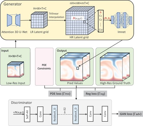
2.2. Generator

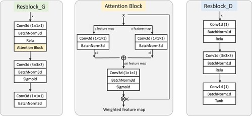
As shown in Figure 2, the generator network consists of two stages. First, an Attention 3D U-Net which is a three-dimensional (3D) variant of the U-Net architecture, which integrates attention gates and residual blocks, is used. As a feature extraction network, it encodes low-resolution input data into an implicit feature grid. The physical constraint network called ‘imnet’ is also used. The U-Net architecture is proposed (Giang et al. 2020) and has been successfully applied to various computer vision tasks, including medical image reconstruction. In contrast to the original U-Net architecture, the 3D U-Net architecture incorporates the attention gate and uses multiple residual blocks (Yu et al. 2017) to improve the training performance of the network. By incorporating the attention gate module, crucial features in the data can be effectively captured. Particularly, the Attention 3D U-Net consists of a contractive part, which combines multiple downsampling modules, and an expansive part, which combines multiple upsampling modules. The design details are given in Table 1.

Figure 2. The generator structure. The generator integrates the attention gate modules and residual blocks and incorporates decoding networks related to physical constraints to enhance the reliability and accuracy of super-resolution predictions of the original physical quantities.

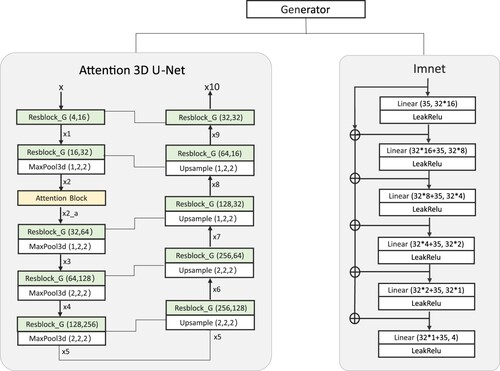
Table 1. The design details of the Attention 3D U-Net.

Input (C  ×  T  ×  H  ×  W)	Operator	Out_channel	Parameter
x0 (4  ×  4  ×  16  ×  16)	ResBlock_G	16	–
x1 (16  ×  4  ×  16  ×  16)	ResBlock_G + MaxPool3d	32	(1,2,2)
x2 (32  ×  4  ×  8  ×  8)	Attention gate module	32	–
x2_a (32  ×  4  ×  8  ×  8)	ResBlock_G + MaxPool3d	64	(1,2,2)
x3 (64  ×  4  ×  4  ×  4)	ResBlock_G + MaxPool3d	128	(2,2,2)
x4 (128  ×  2  ×  2  ×  2)	ResBlock_G + MaxPool3d	256	(2,2,2)
x5 (256  ×  1  ×  1  ×  1)	ResBlock_G + Upsample	128	(2,2,2)
x6 (128  ×  2  ×  2  ×  2)	cat (x6, x4)	256	–
x6' (256  ×  2  ×  2  ×  2)	Upsample + ResBlock_G	64	(2,2,2)
x7 (64  ×  4  ×  4  ×  4)	cat (x7, x3)	128	–
x7' (128  ×  4  ×  4  ×  4)	Upsample + ResBlock_G	32	(1,2,2)
x8 (32  ×  4  ×  8  ×  8)	cat (x8, x2)	64	–
x8' (64  ×  4  ×  8  ×  8)	Upsample + ResBlock_G	16	(1,2,2)
x9 (16  ×  4  ×  16  ×  16)	cat (x9, x1)	32	–
x9' (32  ×  4  ×  16  ×  16)	ResBlock_G	32	–
x10 (32  ×  4  ×  16  ×  16)	output	32	–

The ‘imnet’ represents a physical constraint network. To provide more reliable and accurate super-resolution predictions, this study incorporates knowledge about physical laws into the prediction process rather than relying solely on visual results. In the proposed network design, the input consists of a combination of spatio-temporal position coordinates and their implicit feature vectors. After decoding by the physical constraint network, high-resolution predictions of the original physical quantities are obtained.

• Attention gate block: In the contractive part, an attention gate is introduced. This module involves two input feature maps: the global feature map g and the local feature map x. First, the input feature maps are mapped to the same feature space using convolutional operations to extract shallow features. Next, these two feature maps are merged and processed by the ReLU activation function to obtain the fused feature map, which enhances the signal of the region of interest. Then, an attention weight map is generated by a convolutional layer and a sigmoid activation function. Finally, the input feature map x is multiplied by the attention weight map to yield the weighted feature map as an output. Overall, the attention gate modules can dynamically extract valuable feature information and enhance the network's focus on crucial features by learning the correlations and significance of the input feature maps.

• Contractive part: The contractive part of Attention 3D U-Net consists of multiple downsampling modules and residual block. As shown in Figure 3, the attention gate block is incorporated into the residual block, enabling the network to extract useful feature information adaptively and enhancing its focus on important features. The downsampling modules gradually reduce the spatial resolution of the input volume while increasing the number of feature channels to extract higher-level abstract features. Therefore, four sub-layers denoted by DownLayer1-4 are used to constitute the downsampling modules. Each sub-layer comprises a residual block and a 3D max pooling layer. DownLayer1 and DownLayer2 use a $2\times 2$ pooling window in the width and height dimensions to select the maximum value in each window as the output result, and each depth layer remains unchanged. The attention block is also introduced after the first sub-layer DownLayer1 to enhance the network's performance and expressive power. Then, the output results are fed into the second sub-layer DownLayer2. In DownLayer3 and DownLayer4, a $2\times 2\times 2$ pooling window is used for the input data, with the pooling window size being $2\times 2\times 2$ in the width, height, and depth dimensions. The maximum value in each window is selected as an output result. In short, the downsampling layer reduces the spatial size of the input data through downsampling operations and performs feature extraction using different output channel numbers.

• Expansive part: The expansive part of Attention 3D U-Net is composed of residual block and multiple upsampling modules consisting of a residual convolutional block and an 3d upsampling layer. Each layer connects the feature map of the previous layer with the corresponding feature map of the contractive part to fuse different levels and sizes of feature information. Accordingly, four sub-layers are designed and denoted by UpLayer1-4 to constitute the upsampling modules. Each layer consists of a upsampling layer and a residual block. In UpLayer1 and UpLayer2, a $2\times 2\times 2$ scale_factor is used for the input data. In UpLayer3 and UpLayer4, a $1\times 2\times 2$ scale_factor is used for the input data. In short, the upsampling modules enlarges the spatial size of the feature map through upsampling operations, which is helpful for reconstructing images and expanding features.

The physical constraint network consists of fully connected layers, and the residual idea is adopted in its overall structure. The operational principle of the physical constraint network ($N_{\mathrm{PCN}}$) is explained in detail below. The general form of the nonlinear partial differential equation for the flow simulation in the ocean field is expressed by: (1) $\varphi (t,x,f,f_t,f_x,f_{\mathrm{xx}},\dots )=0$(1) where ϕ is a nonlinear function of time t, space x, function f, and its partial derivatives concerning t, x; subscript of f represents a specific variable of its partial derivative. for instance, $f_{\mathrm{xx}}$ represents the second-order partial derivative of x. However, solving f based on the function ϕ, initial conditions, and boundary conditions is challenging. In view of that, inspired by the TransFlowNet (X. Wang et al. 2022) and MeshfreeFlowNet (Esmaeilzadeh et al. 2020), this study constructs a physical constraint network capable of generating the final high-resolution prediction output $D_{\mathrm{HR}}$. The mathematical representation is as follows: (2) $D_{\mathrm{HR}}\left(P_i\right)=N_{\mathrm{PCN}}(S_i,P_i)=N_{\mathrm{PCN}}\left(G_{\mathrm{HR}}\right(P_i),P_i)$(2) where $S_i$ is the implicit feature vector representing the high-resolution implicit feature grid $G_{\mathrm{HR}}$ at the normalized spatio-temporal coordinate $P_i$; it can decode each $S_i$ into the corresponding original physical variable values in the input data $D_{\mathrm{LR}}$, as shown in Figure 1, an implicit feature vector $S_i$ and its normalized spatio-temporal coordinate $P_i$ form an input vector; $S_i$ is a parameter that is time-related to t and position-related to x and z; $P_i$ represents an arbitrary location in the high-resolution output. We do not impose boundaries and initial conditions in the training of AttGAN. This study does not impose boundary and initial conditions in the training process of the AttGAN model, which enhances the applicability to the same physical system under different conditions. After performing the physical constraint network once, the expected values of the original physical variable at specific positions in the high-resolution output can be obtained. By using backpropagation, the spatio-temporal partial derivatives of the physical variables can be easily computed. When f, $f_x$, and $f_{\mathrm{xx}}$ are obtained, function ϕ could produce the residue of PDEs to contribute physical constraints, which will be used to construct the PDE loss function.

Figure 3. Basic blocks in the generator and discriminator.

2.3. Discriminator

As shown in Figure 4, the discriminator includes the residual convolutional blocks and a self-attention module. The self-attention module is used to focus on features that are more relevant to the input data. The residual block contains skip connections (He et al. 2016; Huang et al. 2017; S. Xie et al. 2017) and nonlinear transformations, which enhances the expressive ability of the discriminator network. As mentioned before, the discriminator distinguishes between the predicted data and the ground truth based on the prominent features. Particularly, the overall design of the discriminator is based on convolutional operations and incorporates a self-attention module to capture the correlations between features. The tensor output by the self-attention layer is processed by the convolutional layer with a kernel size and stride of one. Subsequently, the intermediate output is fed to the residual block, which consists of three convolutional layers, three batch normalization layers, and three nonlinear activation functions. In the proposed design, 32 residual blocks are used to facilitate feature learning. The output of each residual block is processed separately by a $3\times 3$ convolutional layer with a stride of 1 and a $1\times 1$ convolutional layer with a stride of 1. Finally, the output is used to assess the authenticity of the predicted value compared to the ground truth.

Figure 4. The discriminator network architecture.

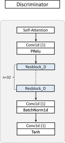
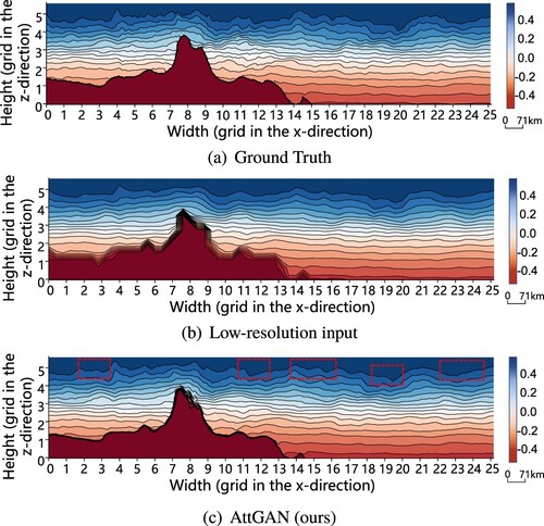
Figure 5. The visualization of salinity at t = 167 T of the ISWs in the South China Sea predicted by AttGAN. Each grid on the axis represents 71 km. The red dashed box in (c) indicates the more prominent waveform features of the ISWs. (a) Ground Truth. (b) Low-resolution input and (c) AttGAN (ours).

2.4. Loss function

The loss function used in this study represents a combination of a regression loss, a PDE loss, and an adversarial loss. During the data preparation stage, high-resolution ground truth data are generated by numerical simulation. At the beginning of each epoch, several data blocks are cropped from the ground truth data as a training dataset. Then, each data block is downsampled eight times to obtain low-resolution data, which are used as input to the generator network. The average loss is calculated for each batch, and the L1 function is used in a definition of the prediction difference loss function. The adversarial loss is used to improve the reconstruction quality and visual perception of the ocean data. Meanwhile, the PDE loss further guides the model to reconstruct data accurately, following the requirements of physical laws. During model training, the AttGAN's parameters are optimized by minimizing the total loss.

2.4.1. Regression loss

The regression loss (X. Wang et al. 2022) measures the difference between the predicted output data and the ground truth data. In this study, it is considered that the batch size of the data blocks sampled from the training data is B. For the $i_{\mathrm{th}}$ spatio-temporal coordinate $P_i$ of the $j_{\mathrm{th}}$ data block $B_j$, we retrieve the corresponding position from the high-resolution ground truth data $D_{\mathrm{GT}}$. The regression loss is calculated by computing the L1 norm between the predicted output data $D_{\mathrm{HR}}$ and the ground truth data $D_{\mathrm{GT}}$ for each position in each data block, taking the average. The regression loss is defined as follows: (3) ${\mathrm{\Gamma }}_{\mathrm{Reg}}=\frac{1}{\left|B\right|}\sum _{j\in B}\left(\frac{1}{\left|B_j\right|}\sum _{i\in B_j}{\Vert D_{\mathrm{HR}}\left(P_i\right)-D_{\mathrm{GT}}\left(P_i\right)\Vert }_1\right)$(3)

2.4.2. PDE loss

The PDE loss (X. Wang et al. 2022) controls the norm of the residual of the PDE, and the scaling coefficient alpha pde weights it. Therefore, it is necessary to achieve a balance between the model structure and the physical constraints to ensure the best super-resolution performance. The PDE loss function ${\mathrm{\Gamma }}_{\mathrm{PDE}}$ is calculated by a differentiable MLP. Accordingly, for a batch of data blocks, ${\mathrm{\Gamma }}_{\mathrm{PDE}}$ is defined as follows: (4) ${\mathrm{\Gamma }}_{\mathrm{PDE}}=\frac{1}{\left|B\right|}\sum _{j\in B}(\frac{1}{\left|B_j\right|}\sum _{i\in B_j}\Vert \varphi (P_i\left){\Vert }_1\right)$(4)

2.4.3. Adversarial loss

The adversarial loss is addressed by alternately optimizing the generator and discriminator networks to solve the adversarial min-max problem. Through the adversarial training approach, the generator continuously learns how to generate realistic ocean data, and the discriminator improves the network's ability to distinguish them from the ground truth. Ultimately, the generator can generate super-resolution results with better perceptual quality, which cannot be directly measured by the pixel error. The adversarial loss is defined by: (5) ${\mathrm{\Gamma }}_{\mathrm{adv}}=\underset{G}{min}\underset{D}{max}{\mathbb{E}}_{x\sim {\mathbb{P}}_{\mathrm{GT}}}[\log D(x\left)\right]+{\mathbb{E}}_{\tilde{x}\sim {\mathbb{P}}_{\mathrm{HR}}}[\log (1-D\left(\tilde{x}\right)\left)\right]$(5) where ${\mathbb{P}}_{\mathrm{GT}}$, ${\mathbb{P}}_{\mathrm{HR}}$ represent the distributions of real and generated data, respectively; $D\left(\tilde{x}\right)$ is the probability that the reconstructed image $D_{\mathrm{HR}}$ is a natural $D_{\mathrm{GT}}$ image.

Finally, the total loss represents the weighted sum of the three loss terms, and α, β, and γ are the weight coefficients of the regression function, PDE function, and adversarial loss function, respectively. During the model training process, the parameters of the AttGAN model are optimized by minimizing the total loss, which is expressed by: (6) ${\mathrm{\Gamma }}_{\mathrm{Tot}}=\alpha {\mathrm{\Gamma }}_{\mathrm{Reg}}+\text{β}{\mathrm{\Gamma }}_{\mathrm{PDE}}+\gamma {\mathrm{\Gamma }}_{\mathrm{adv}}$(6)

3. Experiments

The proposed method was implemented and evaluated on two datasets: the ISWs dataset and the Rayleigh–Bénard convection dataset. To assess the performance of the proposed approach, this study conducted both qualitative and quantitative analyzes. The qualitative analysis involved visual comparisons, and the quantitative analysis included calculating the average PSNR, SSIM, and Amp MSE for each physical variable. The proposed AttGAN was compared with three previous works, and all approaches were trained on the two datasets. In addition, ablation studies were conducted to demonstrate the importance of critical modules in the AttGAN-based super-resolution.

3.1. Oceanic internal solitary waves

3.1.1. Problem description

The ISWs denote a type of underwater wave commonly observed in stratified media in the ocean. They occur between layers of water with different densities, and density differences between the layers primarily drive the ISWs formation. When there is a significant density difference between the layers, the upper layer sinks downward while the lower layer rises upward, resulting in the formation of ISWs. The characteristics and behavior of these waves are influenced by various factors, such as terrain and tides, which can modify the density gradient and fluid velocity in the medium. Compared to other oceanic phenomena, ISWs exhibit unique physical attributes. A representation of PDEs for the ISWs is as follows: (7) $\frac{\mathrm{\partial }T}{\mathrm{\partial }t}+u\frac{\mathrm{\partial }T}{\mathrm{\partial }x}+w\frac{\mathrm{\partial }T}{\mathrm{\partial }z}-K_T({\left(\frac{{\mathrm{\partial }}^{2}T}{\mathrm{\partial }{x}^2}\right)}^2+{\left(\frac{{\mathrm{\partial }}^{2}T}{\mathrm{\partial }{z}^2}\right)}^2)=0$(7) (8) $\frac{\mathrm{\partial }S}{\mathrm{\partial }t}+u\frac{\mathrm{\partial }S}{\mathrm{\partial }x}+w\frac{\mathrm{\partial }S}{\mathrm{\partial }z}-K_S({\left(\frac{{\mathrm{\partial }}^{2}S}{\mathrm{\partial }{x}^2}\right)}^2+{\left(\frac{{\mathrm{\partial }}^{2}S}{\mathrm{\partial }{z}^2}\right)}^2)=0$(8) (9) $\frac{\mathrm{\partial }u}{\mathrm{\partial }x}+\frac{\mathrm{\partial }w}{\mathrm{\partial }z}=0$(9)

The key physical variables associated with ISWs include temperature (T), salinity (S), and velocity components (u, w) in the x and z directions. The above equations correspond to the temperature diffusion equation, the salinity diffusion equation, and the continuity equation, where $K_T$ and $K_S$ denote coefficients of temperature diffusion and salinity diffusion. The above equations can also serve as a physical constraint.

3.1.2. Implementation details

The ISWs dataset was a three-dimensional dataset consisting of two spatial dimensions and one temporal dimension t, organized in the $t\times x\times z$ format. Particularly, this dataset was generated with the spatio-temporal dimension of $192\times 512\times 128$. Through the variation of terrain and tidal coefficients, five sets of datasets were generated, of which four were used for training, and the remaining one was used for evaluation. To ensure the versatility of our network across different dimensions, the evaluation was also performed on the South China Sea dataset, which is illustrated in Figure 5. This dataset was resized to dimensions of $256\times 504\times 120$ ($T\times W\times H$). Further, two-dimensional experiments were performed on an observed dataset of ISWs, as presented in Figure 6, with dimensions set to $64\times 48$ ($T\times H$).

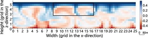
Figure 6. The visualization results of temperature at any point in time in the observation of the ISWs predicted by the proposed AttGAN model. The red dashed box in (c) indicates the more prominent waveform features of the ISWs, which are missing from the low-resolution input. (a) Low-resolution input of temperature channel. (b) Ground Truth and (c) AttGAN (ours).

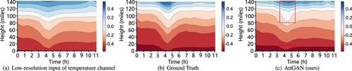
Figure 7. Low-resolution input of temperature channel. Each grid on the axis represents 4 m.

During the training phase, the low-resolution data were used as input data to the generator network. First, the Attention 3D U-Net in the generator was used to obtain an implicit feature vector. In this process, shallow and deep features were concatenated in the channel dimension, with an input channel dimension of four, whereas the output channel dimension is 32. Subsequently, the ‘imnet’ was employed to concatenate the implicit feature vector with spatio-temporal coordinates, which facilitated the solution of differential terms in partial differential equations. The input channel dimension of the decoder was 35 (32 for feature vectors and three for spatio-temporal coordinates), and the output channel dimension was four (four physical variables). The implicit feature vector was decoded to obtain the predicted values at the corresponding spatio-temporal coordinates. Ultimately, the discriminator was applied to evaluate the predicted values further, and the generator and discriminator networks operated cooperatively. The generator network aimed to generate realistic predicted values, making it challenging for the discriminator to judge their authenticity accurately. Meanwhile, the discriminator network attempted to distinguish between the predicted values generated by the generator and the ground truth. The performance of the generator and discriminator gradually improved with the training iteration number.

The training process adopted the Adam optimizer to optimize the model parameters, using a learning rate of 0.001 for 100 epochs. In each epoch, 3000 data blocks were randomly selected for training. The implicit feature grid in the model comprised 512 sample points, representing discrete positions within the flow field. To ensure compliance with the physical equations, an optimal PDE weight coefficient of 0.0125 was used during the training process. In addition, consistency in training settings was maintained across all methods to enable result comparability. In the training process, three loss functions were employed. First, the regression loss (L1) quantified the discrepancy between the predicted values and the ground truth. Second, the PDE loss facilitated the model's understanding of the physical equations and ensured their alignment with the data. Finally, the adversarial loss contributed to enhancing the quality of the super-resolved data by jointly training the generator and discriminator networks.

3.1.3. Evaluation metrics

To evaluate the quality of the proposed method quantitatively, this study selected three metrics, including PSNR (Ledig et al. 2017), SSIM (Ledig et al. 2017), and physical metric Amp MSE (Yuan, Grimshaw, and Johnson 2018), as shown in Table 2, where the best and second-best performances are marked in red and blue colors, respectively.

Table 2. Quantitative comparisons of different methods on ISWs.

The evaluation metrics are as follows:

(1)	PSNR. The peak signal-to-noise ratio (PSNR) considered the magnitude of the image signal-to-noise ratio, and a higher PSNR value indicated a smaller error between the reconstructed image and the original image;
(2)	SSIM. The structural similarity index (SSIM) could be considered a structured method attempting to simulate human perception of image quality; a higher SSIM value indicated a higher similarity between the reconstructed and original images;
(3)	Amp MSE. The amplitude MSE (Amp MSE) referred to the mean square error of the amplitude, which denoted an essential characteristic of ISWs. It measured the accuracy of waveform information, and a lower amplitude MSE suggested a better reconstruction quality for the waveform. By integrating the modal function $S_n$ with the vertical range of motion and the potential function from the seafloor to the sea surface, an approximate expression for the amplitude ${\mathrm{\Lambda }}_n$ of each mode was obtained as follows (Yuan, Grimshaw, and Johnson 2018): (10) ${\mathrm{\Lambda }}_n{S}_n\approx c_n{\displaystyle {\int }_{-h}^{0}u\frac{\mathrm{\partial }{\varphi }_n}{\mathrm{\partial }z}\mathrm{d}z}$(10)

3.1.4. Results comparison

Table 2 presents the quantitative comparison results of different methods, including the traditional trilinear interpolation algorithm, the MeshfreeFlowNet model, and the TransFlowNet model. As shown in Table 2, compared to the MeshfreeFlowNet and TransFlowNet models, the proposed model achieved better performance, having the best average PSNR and SSIM and lowest Amp MSE among all the models (Yuan, Grimshaw, and Johnson 2018). This study also conducted visual comparisons by visualizing sliced data of the temperature component. Figure 7 is low-resolution input of temperature channel. As shown in the red dashed box in Figure 7, compared to the other models, the proposed AttGAN exhibited waveform features that were closer to the ground truth data; meanwhile, the other two models showed noticeable deviations in waveform restoration. This demonstrated the improvement in the overall performance achieved by the proposed attention gate module. Due to its ability to focus more on learning relevant waveform features, the AttGAN could effectively restore waveform details much better than the other models. Considering ISWs' physical significance, the high-resolution data predicted by the proposed model could capture the slight structures and nonlinear effects of waves in the oceanic ISWs dataset. However, in low-resolution inputs, only the overall morphology of the waves could be observed, which might affect the understanding and prediction of the wave behavior. Further, a detailed investigation of the ISWs in the South China Sea was conducted. The results showed that for the proposed method, it was possible to target input data of various types and sizes. Unlike the dataset used previously, the dimensions of the South China Sea dataset were $256\times 504\times 120$ ($T\times W\times H$). The visual results are shown in Figure 5. The red dashed box in Figure 5(c) showed that the waveform features of the high-frequency detail lost in the low-resolution data could be recovered well by the proposed model; namely, the waveform was very close to the ground truth. Further, to enhance authenticity and persuasiveness, additional observational data of the ISWs were collected to validate the proposed approach. The training process included seven sets of training data and one set of evaluation data. The dimensions of observational data of the ISWs were resized to $64\times 48$ ($T\times H$). As discerned from the annotated red boxes in Figure 6(c), the proposed network could successfully recover the missing wave features present in the observational data from the low-resolution input. This indicated that the proposed network exhibited favorable performance. Overall, improvements from the comparative experiment and supplementary experiments could be observed, which demonstrated the enhanced robustness and generalization capability of the AttGAN after adversarial training.

Figure 8. Visual comparisons of different methods for the temperature at t = 82 T, including the ground truth, the proposed model's result, the MeshFreeFlowNet model's result, and the TransFlowNet model's result. Each grid on the axis represents 3 km. The red dashed box reveals differences in the restored waveform features between the three models. The proposed model's result was the closest to the ground truth, followed by the MeshFreeFlowNet model. (a) Ground Truth. (b) AttGAN (ours). (c) MessFreeFlowNet and (d) TransFlowNet.

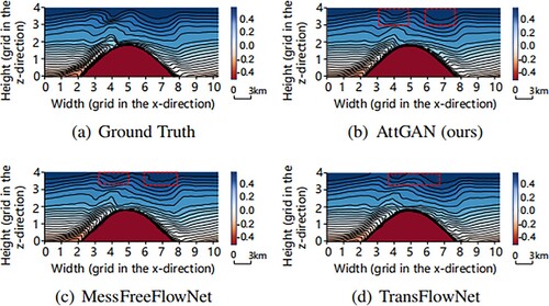
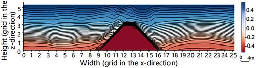
Figure 9. Low-resolution input of temperature channel. Each grid on the axis represents 80 m.

3.2. Rayleigh–Bénard convection problem

3.2.1. Problem description

The Rayleigh–Bénard convection problem (Esmaeilzadeh et al. 2020) represents a classical fluid mechanics problem that primarily describes the motion of a fluid confined between two horizontal plates, where one plate is heated, and another is cooled, which creates a temperature difference. First, the fluid is constrained between the two plates, with the upper (lower) plate being kept hot (cold); the fluid adjacent to the hot (cold) plate experiences a gradual temperature rise (drop). This thermal discrepancy induces buoyancy effects, increasing density gradients, vortices, and turbulence. As instability intensifies, the flow progresses into a chaotic and turbulent state. Commonly referred to as the two-dimensional Rayleigh–Bénard instability problem, the simulation of this phenomenon encompasses four key physical variables: pressure (P), temperature (T), and velocity components (u, w) along the x and z directions.

3.2.2. Implementation details

Data Generation: This study used the Dedalus framework (Burns et al. 2020) to solve the partial differential equations numerically and generated high-resolution ground truth data with a size of $192\times 512\times 128$ ($T\times W\times H$) by numerical simulations. The temperature difference between the upper and lower plates was set at $1K$, with a Rayleigh number of $1\times {10}^6$ and a Prandtl number of one. In addition, the aspect ratio in the z direction was 4, meaning the length of the plates was 4m, with a spacing of 1m. Similar to the training process mentioned in the ISWs, at the beginning of each epoch, several data blocks with a size of ($16\times 128\times 128$) were cropped from the ground truth data to form the training dataset for that epoch. Each data block was downsampled to $4\times 8\times 8$ ($T\times W\times H$) to serve as low-resolution input data.

3.2.3. Results comparison

Table 3 illustrates a quantitative comparison of the proposed method and the state-of-the-art methods. Compared to the state-of-the-art methods, including the MeshfreeFlowNet model, the TransFlowNet model, and the traditional trilinear interpolation model, the proposed AttGAN demonstrates superior performance, having the highest average PSNR and SSIM values among all the methods. In addition, Figure 9 is low-resolution input of temperature channel and visual comparison results obtained using sliced data from the temperature component are depicted in Figure 10. The results revealed that the images generated by the proposed AttGAN closely resembled the ground truth. In comparison, the TransFlowNet and MeshfreeFlowNet models exhibited artifacts despite their proximity to the ground truth. Similarly, considering its physical significance, the high-resolution data predicted by the proposed model revealed the complex dynamics and microstructures of convective vortices, while low-resolution inputs could only display the macroscopic features of the flow field. This could further lead to misunderstandings of system dynamics and stability, as well as inaccurate modeling of chaotic phenomena. Finally, this fully proved the robustness and good generalization of the proposed AttGAN model based on the attention gate module.

Figure 10. Visual comparison results of different methods for the temperature component at $t=92$ T. Each grid on the axis represents 6 m. Compared to the ground truth, the result of the MessFreeFlowNet exhibited noticeable biases (particularly in the lower center of the vortex on the left). The TransFlowNet introduced some grid-like artifacts, and the proposed AttGAN achieved the best result among all the models. (a) Ground Truth. (b) AttGAN (ours). (c) MessFreeFlowNet and (d) TransFlowNet.

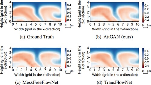
Table 3. Quantitative comparisons of different methods on Rayleigh–Bénard.

3.3. Ablation study

This section presents ablation experiments performed using the proposed network on the ISWs datasets to evaluate the impact of four important design modules of the proposed model. As shown in Table 4, first, the results of the baseline were listed, and then the ablation was performed on each of the four modules separately.

Table 4. Ablation study results of AttGAN using the ISWs dataset.

Design	S		T		u		w		Average
	PSNR	SSIM	PSNR	SSIM	PSNR	SSIM	PSNR	SSIM	PSNR	SSIM	Amp MSE
AttGAN (alpha = 0.0125)	33.9192	0.9926	39.6518	0.9936	43.6542	0.9879	44.9015	0.9897	40.5317	0.9909	0.0889
No_attBlock	33.1368	0.9915	38.4394	0.9924	44.1019	0.9883	44.3956	0.9890	40.0184	0.9903	0.0843
No_G_resblock	32.5625	0.9908	37.8966	0.8740	42.2621	0.9747	42.2488	0.9997	38.7425	0.9598	0.1833
No_D_resblock	32.3296	0.9920	39.8961	0.9935	43.4066	0.9879	44.8158	0.9893	40.1120	0.9907	0.1181
pde_alpha = 0.0	32.4331	0.9916	39.1179	0.9930	44.0051	0.9881	44.5461	0.9892	40.0256	0.9905	0.0955
pde_alpha=0.01	32.6950	0.9919	38.9379	0.9927	43.2541	0.9869	44.2651	0.9886	39.7880	0.9900	0.1340
pde_alpha=0.03	33.0056	0.9917	38.2447	0.9918	42.9394	0.9868	44.5880	0.9890	39.6945	0.9898	0.1592
pde_alpha=0.05	33.3694	0.9924	37.6176	0.9897	43.0222	0.9876	44.6612	0.9893	39.6676	0.9897	0.1026
pde_alpha=0.07	34.0656	0.9928	35.8669	0.9853	42.7689	0.9857	44.4598	0.9891	39.2903	0.9882	0.1443

3.3.1. Attention gate module

First, the effectiveness of the attention gate module in the generator network was demonstrated. The ‘No_attBlock’ row in Table 4 represents the proposed network model where only the attention gate module was removed, while the rest of the network remained unchanged. As shown in Table 4, without the attention gate module, the average PSNR and SSIM were reduced by 1.27% and 0.06%, respectively. This has indicated that the attention gate module plays an important role in early visual processing and can help to achieve better results in subsequent network layers, especially in terms of PSNR.

3.3.2. Residual block

Attention 3D U-Net in the generator is based on the U-Net architecture (Agrawal, Katal, and Hooda 2022; Esmaeilzadeh et al. 2020; S. Guo et al. 2023; Nguyen et al. 2020), which incorporates a multilevel residual structure and skip connections. This allows it to better integrate features. Residual connections help to alleviate the vanishing gradient problem and make the network easier to optimize. These connections enable the network to learn residual mappings directly, thus facilitating more effective gradient propagation and learning of complex feature representations. Meanwhile, skip connections allow a direct combination of low- and high-level features and enable the network to leverage feature representations at different levels, thus better extracting multi-scale information. Next, when some residual blocks were removed while the rest of the network was unchanged, as shown in Table 4, it could be observed that without these residual blocks, the average PSNR and SSIM decreased by 4.41% and 3.13%, respectively, whereas the Amp MSE increases by 0.0944. Correspondingly, the discriminator network is designed in a convolutional form, and the backbone network consists of 32 residual blocks to learn features more effectively. Next, these residual convolutional blocks were removed while the rest of the network was unchanged. As shown in Table 4, without these residual blocks, the average PSNR and SSIM were reduced by 1.03% and 0.02%, respectively, and the Amp MSE was increased by 0.0292.

3.3.3. Physical constraints

Finally, the effect of the weighted PDE loss term with a hyperparameter pde alpha was investigated. As shown in Table 4, $\mathrm{pde}\mathrm{\_alpha}\in \{0,0.01,0.03,0.05,0.07\}$ was used in this analysis. The AttGAN's performance changed when the PDE loss was considered, but larger pde_alpha values did not always yield better results. This was because the physical constraints were additional. The PDE loss helped reconstruct local features. We found a balance through experiments and obtained an optimal performance with pde_alpha = 0.0125. Furthermore, when pde_alpha was equal to 0, only based on regression loss and adversarial loss, without considering the physical constraints on the predicted high-resolution data, the average PSNR and SSIM were lower and the Amp MSE was higher. The results indicated that the PDE loss still has a certain degree of influence on the results.

4. Limitations and discussions

Based on the aforementioned experimental results, it could be concluded that traditional trilinear interpolation algorithms and previously proposed well-performing neural network models (such as MeshFreeFlowNet and TransFlowNet models) are not as effective as the proposed AttGAN model in addressing the spatio-temporal super-resolution challenges associated with the ocean data. This suggests that conventional methods cannot solely rely on raw deep learning-based models to tackle the problem considered in this work, whereas deep learning-based frameworks that integrate the attention gate and physical constraints can effectively overcome this challenge. As presented in Figure 11 even when the ground truth data are spatially downsampled by a factor of 16, the proposed AttGAN model could maintain exceptional performance. However, the proposed model has certain limitations. First, when subjected to data downsampled by a factor of 32, the AttGAN could not yield satisfactory results. This might be attributed to the proposed model's inability to capture adequate detailed information under higher levels of downsampling, which could consequently result in performance degradation. Second, the proposed AttGAN model comprises 1.8 million parameters, and despite its substantial parameter size, the inference process remains relatively swift. Therefore, in future endeavors, enhancing the proposed model's architecture and algorithm could be considered to address the mentioned limitations and enhance the model's performance in more intricate scenarios.

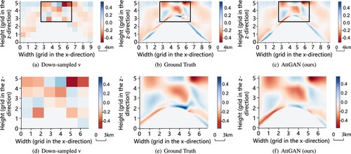
Figure 11. Visualization results of slices of velocity component v ($\times 16$) at t = 41 T predicted by the proposed AttGAN. In (a)–(c), each grid on the axis represents 4 km; in (d)–(f), each grid on the axis represents 3 km. The result predicted by the proposed model was close to the ground truth. (a) Down-sampled v. (b) Ground Truth. (c) AttGAN (ours). (d) Down-sampled v. (e) Ground Truth and (f) AttGAN (ours).

5. Conclusion

This paper introduces an innovative deep learning-based framework for spatio-temporal super-resolution of ocean phenomena named AttGAN. The generator of the proposed AttGAN includes attention gate modules, residual convolutional blocks, and physical constraints represented by the PDE. By establishing a loss function that combines a regression loss, a PDE loss, and an adversarial loss, the AttGAN model is trained with strong generalization ability. The experimental results demonstrate the excellent performance of the AttGAN model on the ISWs and Rayleigh–Bénard convection dataset. Moreover, the results show that the AttGAN can outperform traditional trilinear interpolation and deep learning-based frameworks in terms of super-resolution effect. Finally, the proposed network and the results presented in this study could facilitate the related research and accelerate the processing of data super-resolution problems.

Disclosure statement

No potential conflict of interest was reported by the author(s).

Data availability statement

The data that support the findings of this study are openly available in Zenodo at https://doi.org/10.5281/zenodo.10472771

 Google Scholar

.

Additional information

Funding

Xinjie Wang was supported by the National Key R&D Program of China (Grant No. 2022YFC2803805), the Fundamental Research Funds for the Central Universities (Grant No. 202313035), and the Shandong Provincial Natural Science Foundation of China (Grant No. ZR2021QF124). Chunxin Yuan was supported by the National Natural Science Foundation of China (Grant No. 42006016), the Fundamental Research Funds for the Central Universities (Grant No. 202265005, Grant No. 202264007), the key program of the National Natural Science Foundation of China (Grant No. 91958206), the State Key Laboratory of Tropical Oceanography, South China Sea Institute of Oceanology, Chinese Academy of Sciences (Project Grant No. LTO2303), the Natural Science Foundation of Shandong Province (Grant No. ZR2020QD063), and Jie Nie was supported by the National Natural Science Foundation of China (Grant No. U23A20320).

References

- Agrawal, P., N. Katal, and N. Hooda. 2022. “Segmentation and Classification of Brain Tumor Using 3D-UNet Deep Neural Networks.” International Journal of Cognitive Computing in Engineering 3:199–210. https://doi.org/10.1016/j.ijcce.2022.11.001.
- Arora, R. 2022. “PhySRNet: Physics Informed Super-Resolution Network for Application in Computational Solid Mechanics”. In 2022 IEEE/ACM International Workshop on Artificial Intelligence and Machine Learning for Scientific Applications (AI4S), 13–18. IEEE. https://doi.org/10.1109/ai4s56813.2022.00008.
- Br, P., and N. Rajkumar. 2024. “Real-Time Intelligent Video Surveillance System Using Recurrent Neural Network.” Procedia Computer Science 235:1522–1531. https://doi.org/10.1016/j.procs.2024.04.143.
- Burns, K. J., G. M. Vasil, J. S. Oishi, D. Lecoanet, and B. P. Brown. 2020. “Dedalus: A Flexible Framework for Numerical Simulations with Spectral Methods.” Physical Review Research 2 (2): 023068. https://doi.org/10.1103/physrevresearch.2.023068.
- Jiang C., S. Esmaeilzadeh, K. Azizzadenesheli, K. Kashinath, M. Mustafa, H. A. Tchelepi, P. Marcus, M. Prabhat, and A. Anandkumar. 2020. “Meshfreeflownet: A Physics-Constrained Deep Continuous Space–Time Super-Resolution Framework.” In SC20: International Conference for High Performance Computing, Networking, Storage and Analysis, 1–15. IEEE. https://doi.org/10.1109/sc41405.2020.00013.
- Chakraborty, T., U. R. KS, S. M. Naik, M. Panja, and B. Manvitha. 2024. “Ten Years of Generative Adversarial Nets (GANs): A Survey of the State-of-the-Art.” Machine Learning: Science and Technology5 (1): 011001. https://doi.org/10.1088/2632-2153/ad1f77.
- Cole, E. K., F. Ong, S. S. Vasanawala, and J. M. Pauly. 2021. “Fast Unsupervised MRI Reconstruction Without Fully-Sampled Ground Truth Data Using Generative Adversarial Networks”. In Proceedings of the IEEE/CVF International Conference on Computer Vision, 3988–3997. https://doi.org/10.1109/iccvw54120.2021.00444.
- Edwards, C. A., A. M. Moore, I. Hoteit, and B. D. Cornuelle. 2015. “Regional Ocean Data Assimilation.” Annual Review of Marine Science 7 (1): 21–42. https://doi.org/10.1146/annurev-marine-010814-015821.
- Fujii, Y., E. Rémy, H. Zuo, P. Oke, G. Halliwell, F. Gasparin, M. Benkiran. 2019. “Observing System Evaluation Based on Ocean Data Assimilation and Prediction Systems: On-Going Challenges and a Future Vision for Designing and Supporting Ocean Observational Networks.” Frontiers in Marine Science 6:417. https://doi.org/10.3389/fmars.2019.00417.
- Gao, H., L. Sun, and J.-X. Wang. 2021. “Super-Resolution and Denoising of Fluid Flow Using Physics-Informed Convolutional Neural Networks Without High-Resolution Labels.” Physics of Fluids 33 (7): 073603. https://doi.org/10.1063/5.0054312.
- Giang, T. L., K. B. Dang, Q. T. Le, V. G. Nguyen, S. S. Tong, and V. -M. Pham. 2020. “U-Net Convolutional Networks for Mining Land Cover Classification Based on High-Resolution UAV Imagery.” IEEE Access 8:186257–186273. https://doi.org/10.1109/access.2020.3030112.
- Glawion, L., J. Polz, H. G. Kunstmann, B. Fersch, and C. Chwala. 2023. “spateGAN: Spatio-Temporal Downscaling of Rainfall Fields using a cGAN Approach”. https://doi.org/10.22541/essoar.167690003.33629126/v1.
- Guo, J., and H. Chao. 2017. “Building an End-To-End Spatial-Temporal Convolutional Network for Video Super-Resolution”. In Proceedings of the AAAI Conference on Artificial Intelligence, Vol. 31. https://doi.org/10.1609/aaai.v31i1.11228.
- Guo, S., N. Sun, Y. Pei, and Q. Li. 2023. “3D-UNet-LSTM: A Deep Learning-Based Radar Echo Extrapolation Model for Convective Nowcasting.” Remote Sensing 15 (6): 1529. https://doi.org/10.3390/rs15061529.
- He, K., X. Zhang, S. Ren, and J. Sun. 2016. “Deep Residual Learning for Image Recognition”. In Proceedings of the IEEE Conference on Computer Vision and Pattern Recognition, 770–778. https://doi.org/10.1109/cvpr.2016.90.
- Huang, G., Z. Liu, L. Van Der Maaten, and K. Q. Weinberger. 2017. “Densely Connected Convolutional Networks”. In Proceedings of the IEEE Conference on Computer Vision and Pattern Recognition, 4700–4708. https://doi.org/10.1109/cvpr.2017.243.
- Ismail, M., C. Shang, J. Yang, and Q. Shen. 2023. “Sparse Data-Based Image Super-Resolution with ANFIS Interpolation.” Neural Computing and Applications 35: 7221–7233. https://doi.org/10.1007/s00521-021-06500-x.
- Jagtap, A. D., and G. E. Karniadakis. 2021. “Extended Physics-Informed Neural Networks (XPINNs): A Generalized Space-Time Domain Decomposition based Deep Learning Framework for Nonlinear Partial Differential Equations”. In AAAI Spring Symposium: MLPS, Vol. 10. https://doi.org/10.4208/cicp.oa-2020-0164.
- Jagtap, A. D., E. Kharazmi, and G. E. Karniadakis. 2020. “Conservative Physics-Informed Neural Networks on Discrete Domains for Conservation Laws: Applications to Forward and Inverse Problems.” Computer Methods in Applied Mechanics and Engineering 365:113028. https://doi.org/10.1016/j.cma.2020.113028.
- Jia, S., D. Bi, J. Liao, S. Jiang, M. Xu, and S. Zhang. 2023. “Structure-Adaptive Convolutional Neural Network for Hyperspectral Image Classification.” IEEE Transactions on Geoscience and Remote Sensing 61: 1–16. https://doi.org/10.1109/tgrs.2023.3326231.
- Kappeler, A., S. Yoo, Q. Dai, and A. K. Katsaggelos. 2016. “Video Super-Resolution with Convolutional Neural Networks.” IEEE Transactions on Computational Imaging 2 (2): 109–122. https://doi.org/10.1109/tci.2016.2532323.
- Kearney, V., J. W. Chan, T. Wang, A. Perry, M. Descovich, O. Morin, S. S. Yom, and T. D. Solberg. 2020. “DoseGAN: A Generative Adversarial Network for Synthetic Dose Prediction Using Attention-Gated Discrimination and Generation.” Scientific Reports 10 (1): 11073. https://doi.org/10.1038/s41598-020-68062-7.
- Kharazmi, E., Z. Zhang, and G. E. Karniadakis. 2021. “hp-VPINNs: Variational Physics-Informed Neural Networks with Domain Decomposition.” Computer Methods in Applied Mechanics and Engineering374:113547. https://doi.org/10.1016/j.cma.2020.113547.
- Krizhevsky, A., I. Sutskever, and G. E. Hinton. 2012. “Imagenet Classification with Deep Convolutional Neural Networks.” Advances in Neural Information Processing Systems 60: 84–90. https://doi.org/10.1145/3065386.
- Ledig, C., L. Theis, F. Huszár, J. Caballero, A. Cunningham, A. Acosta, A. Aitken, et al. 2017. “Photo-Realistic Single Image Super-Resolution Using a Generative Adversarial Network”. In Proceedings of the IEEE Conference on Computer Vision and Pattern Recognition, 4681–4690. https://doi.org/10.1109/cvpr.2017.19.
- Li, M., and C. McComb. 2022. “Using Physics-Informed Generative Adversarial Networks to Perform Super-Resolution for Multiphase Fluid Simulations.” Journal of Computing and Information Science in Engineering 22 (4): 044501. https://doi.org/10.31224/osf.io/pu2jx.
- Lim, B., S. Son, H. Kim, S. Nah, and K. Mu Lee. 2017. “Enhanced Deep Residual Networks for Single Image Super-Resolution”. In Proceedings of the IEEE Conference on Computer Vision and Pattern Recognition Workshops, 136–144. https://doi.org/10.1109/cvprw.2017.151.
- Ling, F., Y. Du, X. Li, W. Li, F. Xiao, and Y. Zhang. 2013. “Interpolation-Based Super-Resolution Land Cover Mapping.” Remote Sensing Letters 4 (7): 629–638. https://doi.org/10.1080/2150704x.2013.781284.
- Marechal, G., and F. Ardhuin. 2021. “Surface Currents and Significant Wave Height Gradients: Matching Numerical Models and High-Resolution Altimeter Wave Heights in the Agulhas Current Region.” Journal of Geophysical Research: Oceans 126 (2): e2020JC016564. https://doi.org/10.1002/essoar.10505343.1.
- Nguyen, T. T., T. N. Chi, M. D. Hoang, H. N. Thai, and T. N. Duc. 2020. “3D Unet Generative Adversarial Network for Attenuation Correction of SPECT Images”. In 2020 4th International Conference on Recent Advances in Signal Processing, Telecommunications & Computing (SigTelCom), 93–97. IEEE. https://doi.org/10.1109/sigtelcom49868.2020.9199018.
- Parker, J. A., R. V. Kenyon, and D. E. Troxel. 1983. “Comparison of Interpolating Methods for Image Resampling.” IEEE Transactions on Medical Imaging 2 (1): 31–39. https://doi.org/10.1109/TMI.1983.4307610.
- Qiao, F., W. Zhao, X. Yin, X. Huang, X. Liu, Q. Shu, G. Wang, et al. 2016. “A Highly Effective Global Surface Wave Numerical Simulation with Ultra-High Resolution”. In SC'16: Proceedings of the International Conference for High Performance Computing, Networking, Storage and Analysis, 46–56. IEEE. https://doi.org/10.1109/sc.2016.4.
- Raissi, M., P. Perdikaris, and G. E. Karniadakis. 2019. “Physics-Informed Neural Networks: A Deep Learning Framework for Solving Forward and Inverse Problems Involving Nonlinear Partial Differential Equations.” Journal of Computational Physics 378:686–707. https://doi.org/10.1016/j.jcp.2018.10.045.
- Song, J., H. Yi, W. Xu, X. Li, B. Li, and Y. Liu. 2023. “ESRGAN-DP: Enhanced Super-Resolution Generative Adversarial Network with Adaptive Dual Perceptual Loss.” Heliyon 9 (4): e15134. https://doi.org/10.1016/j.heliyon.2023.e15134.
- Velho, H. F. C., H. C. Furtado, S. B. Sambatti, C. B. O. F. de Barros, M. E. Welter, R. P. Souto, D. Carvalho, and D. O. Cardoso. 2022. “Data Assimilation by Neural Network for Ocean Circulation: Parallel Implementation.” Supercomputing Frontiers and Innovations 9 (1): 74–86. https://doi.org/10.14529/jsfi220105.
- Wang, T.-C., M.-Y. Liu, J.-Y. Zhu, A. Tao, J. Kautz, and B. Catanzaro. 2018. “High-Resolution Image Synthesis and Semantic Manipulation with Conditional GANs”. In Proceedings of the IEEE Conference on Computer Vision and Pattern Recognition, 8798–8807. https://doi.org/10.1109/cvpr.2018.00917.
- Wang, C., Y. Zhang, Y. Zhang, R. Tian, and M. Ding. 2021. “Mars Image Super-Resolution Based on Generative Adversarial Network.” IEEE Access 9:108889–108898. https://doi.org/10.1109/access.2021.3101858.
- Wang, X., S. Zhu, Y. Guo, P. Han, Y. Wang, Z. Wei, and X. Jin. 2022. “TransFlowNet: A Physics-Constrained Transformer Framework for Spatio-Temporal Super-Resolution of Flow Simulations.” Journal of Computational Science 65:101906. https://doi.org/10.1016/j.jocs.2022.101906.
- Waters, J., D. J. Lea, M. J. Martin, I. Mirouze, A. Weaver, and J. While. 2015. “Implementing a Variational Data Assimilation System in An Operational 1/4 Degree Global Ocean Model.” Quarterly Journal of the Royal Meteorological Society 141 (687): 333–349. https://doi.org/10.1002/qj.2388.
- Xie, Y., E. Franz, M. Chu, and N. Thuerey. 2018. “tempoGAN: A Temporally Coherent, Volumetric GAN for Super-Resolution Fluid Flow.” ACM Transactions on Graphics (TOG) 37 (4): 1–15. https://doi.org/10.1145/3197517.3201304.
- Xie, S., R. Girshick, P. Dollár, Z. Tu, and K. He. 2017. “Aggregated Residual Transformations for Deep Neural Networks”. In Proceedings of the IEEE Conference on Computer Vision and Pattern Recognition, 1492–1500 . https://doi.org/10.1109/cvpr.2017.634.
- Xu, J., Y. Chae, B. Stenger, and A. Datta. 2018. “Dense Bynet: Residual Dense Network for Image Super Resolution”. In 2018 25th IEEE International Conference on Image Processing (ICIP), 71–75. IEEE. https://doi.org/10.1109/icip.2018.8451696.
- Yonekura, K., K. Maruoka, K. Tyou, and K. Suzuki. 2023. “Super-Resolving 2D Stress Tensor Field Conserving Equilibrium Constraints Using Physics-Informed U-Net.” Finite Elements in Analysis and Design 213:103852. https://doi.org/10.1016/j.finel.2022.103852.
- Yoon, Y., H.-G. Jeon, D. Yoo, J.-Y. Lee, and I. So Kweon. 2015. “Learning a Deep Convolutional Network for Light-Field Image Super-Resolution”. In Proceedings of the IEEE International Conference on Computer Vision Workshops, 24–32. https://doi.org/10.1109/iccvw.2015.17.
- Yu, L., X. Yang, H. Chen, J. Qin, and P. A. Heng. 2017. “Volumetric ConvNets with Mixed Residual Connections for Automated Prostate Segmentation from 3D MR Images”. In Proceedings of the AAAI Conference on Artificial Intelligence, Vol. 31. https://doi.org/10.1609/aaai.v31i1.10510.
- Yuan, C., R. Grimshaw, and E. Johnson. 2018. “The Evolution of Second Mode Internal Solitary Waves Over Variable Topography.” Journal of Fluid Mechanics 836:238–259. https://doi.org/10.1017/jfm.2017.812.
- Zayats, M., M. J. Zimoń, K. Yeo, and S. Zhuk. 2022. “Super Resolution for Turbulent Flows in 2D: Stabilized Physics Informed Neural Networks”. In 2022 IEEE 61st Conference on Decision and Control (CDC), 3377–3382. IEEE. https://doi.org/10.1109/cdc51059.2022.9992729.
- Zhang, K., L. V. Gool, and R. Timofte. 2020. “Deep Unfolding Network for Image Super-Resolution”. In Proceedings of the IEEE/CVF Conference on Computer Vision and Pattern Recognition, 3217–3226. https://doi.org/10.1109/cvpr42600.2020.00328.
- Zhang, D., L. Guo, and G. E. Karniadakis. 2020. “Learning in Modal Space: Solving Time-Dependent Stochastic PDEs Using Physics-Informed Neural Networks.” SIAM Journal on Scientific Computing 42 (2): A639–A665. https://doi.org/10.1137/19m1260141.
- Zhang, Y., C. Liu, M. Liu, T. Liu, H. Lin, C.-B. Huang, and L. Ning. 2024. “Attention is All You Need: Utilizing Attention in AI-Enabled Drug Discovery.” Briefings in Bioinformatics 25 (1): bbad467. https://doi.org/10.1093/bib/bbad467.