Towards submesoscale eddy detection in SDGSAT-1 data through deep learning

ABSTRACT

In coastal regions, the formation of submesoscale eddies is frequently influenced by factors including topography, tidal forces, and ocean currents. These eddies are often challenging to detect owing to the limited spatial resolution of altimeters and restricted observation areas. Equipped with a multispectral imager (MSI) specialized in coastal and offshore environments, SDGSAT-1 supports the sustainable development goals. It generates extensive data concerning nearshore resources. However, the multispectral data from SDGSAT-1 exhibit image blurring and indistinct eddy boundaries due to the imaging conditions of remote sensing satellites. This challenge impedes conventional deep learning models from directly identifying these features. Consequently, we developed a multispectral eddy detection network (MEDNet). Given the characteristics of remote sensing images, we employ a linear stretching technique to enhance eddy information in SDGSAT-1 images. Additionally, we propose a multispectral eddy horizontal flip technique (MEHFT) to address the imbalance between cyclonic and anticyclonic eddies in remote sensing imagery. To direct the network’s focus towards critical areas, we incorporate a multi-branch stacking construct and an SPPCSPC module to enhance eddy feature extraction. Experimental results demonstrate that our method achieves high accuracy (mAP of 90.42%) in the dataset, surpassing competing object detection models.

KEYWORDS:

• Submesoscale eddy
• SDGSAT-1
• deep learning
• object detection

1. Introduction

Submesoscale eddies, significant small-scale features in the ocean, are characterized by horizontally extended scales ranging from a few kilometers to several tens of kilometers. Typically short-lived, these eddies last only from a few hours to several days (Capet et al. 2008; McWilliams 2019). Influenced by dynamic processes including turbulence and gradient winds, submesoscale eddies typically arise in the marine boundary layer and the adjacent mixed layer, playing vital roles in marine ecological and physical processes (McWilliams 2016; Taylor and Thompson 2023). Additionally, anticyclonic eddies can induce local climatic instabilities, such as increased sea surface wind speeds, humidity, and cloudiness, potentially impacting maritime navigation safety and fishing activities in shipping lanes and offshore areas (Frenger et al. 2013). Therefore, detecting submesoscale eddies contributes to a better understanding of the complexity and interconnectedness of ocean systems.

Initial observations and studies of eddies primarily utilized buoys, submersibles, and altimeters. However, the scarcity of in-situ observation data largely limited oceanic eddy research to describing a few observed phenomena (Cheng, Quan, and Qiang 2005). With advancements in remote sensing satellites, extensive data from satellite altimeters now facilitate the identification and enumeration of ocean eddies across sea areas through changes in sea surface height (SSH), and allow analysis of their primary characteristics, including distribution, spatial scale, and life cycle (Cheng, Quan, and Qiang 2005; Qin et al. 2015). Nevertheless, the limited spatial resolution of satellite altimetry renders the accurate identification of small-scale, short-lived submesoscale eddies unfeasible. To address this challenge, the utilization of additional satellite remote sensing data, such as chlorophyll-a (Chl-a) concentration and sea surface temperature (SST), is necessary (Becker, Romero, and Pisoni 2023; Ni et al. 2021). However, variations in SST and Chl-a concentrations, influenced by diverse factors, may lead to false detections in eddy identification. Consequently, Synthetic Aperture Radar (SAR) has recently become the preferred sensor for detecting submesoscale eddies, due to its high spatial resolution and all-weather imaging capabilities (Ji et al. 2021; Karimova and Gade 2016; Wang and Chong 2020; Xu et al. 2015). Driven by SAR imaging mechanisms, most submesoscale eddies are detected using tracers like bio-oil films and sea ice, or through sea surface roughness induced by shear flows (Karimova 2012). Specifically, eddy features are characterized by distinct bright and dark spiral structures, depending on their mechanisms. These factors make extracting information from oceanic eddies, amid complex marine environments and redundant signal noise, particularly challenging.

However, with advancements in computing and big data, deep learning techniques are now extensively employed in oceanographic research (Ge et al. 2023; Zhang et al. 2022). To address these challenges, deep learning techniques have made significant progress in identifying submesoscale eddies in SAR images. Xia et al. (2022) introduced the submesoscale eddy detection model CEA-Net, based on numerous labeled SAR eddy images and developed alongside the high-resolution Sentinel-1 dataset. Vincent et al. (2023) proposed a semi-supervised framework based on SAR images that enhances the identification of submesoscale oceanic eddies through domain-specific, self-supervised comparative pre-training models fine-tuned on smaller labeled datasets. Zhang et al. (2023) introduced a multi-task learning strategy for the marine eddy detection model EddyDet, aimed at automatically identifying and segmenting individual eddies at the pixel level, with an emphasis on enhancing prediction mask quality. Detailed pixel masks are provided for each object instance, thereby facilitating subsequent tasks such as the inversion of eddy parameters.

The implementation of a submesoscale eddy detection method based on SAR imagery, as proposed, provides a valuable reference for this study. However, compared to multispectral data, SAR offers limited spectral feature information. Additionally, the single polarization feature of SAR cannot fully capture comprehensive sea surface information. For instance, when wind speeds are below a certain threshold, SAR struggles to detect submesoscale eddies using primary tracers such as Chl-a, suspended solids, and algae. The Sustainable Development Goals Scientific Satellite-1 (SDGSAT-1), equipped with a multispectral imager (MSI) that provides rich band information and microstructural features, is uniquely suited to observe submesoscale eddies using tracers such as Chl-a, suspended solids, and algae. Therefore, this study proposes to develop an automated submesoscale eddy detection model based on SDGSAT-1 multispectral data, offering a valuable dataset for further research into submesoscale eddies.

The major contributions of this work are outlined as follows:

1. A manually interpreted submesoscale eddy dataset, SDG-Eddy 2022, has been constructed using SDGSAT-1 multispectral data, providing valuable data resources for further research on submesoscale eddies.

2. To address training sample imbalance, a submesoscale eddy image transformation method (MEHFT) is proposed. Utilizing the same-hemisphere symmetry of submesoscale eddies, the left pixel of the eddy image is swapped with the right pixel, thereby achieving image flipping. This transformation not only balances the counts of cyclonic (CE) and anticyclonic (AE) eddies but also increases the sample size.

3. A submesoscale eddy detection model, MEDNet, is introduced. Detection performance across various scales of eddies is significantly enhanced by improved feature fusion strategies, achieving a mean average precision (mAP) of 90.42%.

The remainder of this paper is organized as follows: Section 2 introduces the preamble, Section 3 details the research methodology, Section 4 presents and discusses the experimental results, and Section 5 concludes the paper.

2. Preliminaries

2.1. Dataset (SDG-Eddy 2022)

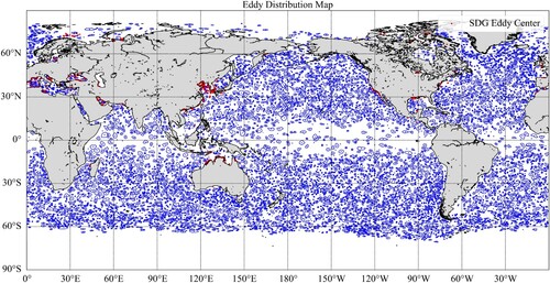
Given that existing altimeter measurements are insufficient for capturing small-scale variations in nearshore oceans, land-based satellites with high spatial resolution have become essential for this area of research. The SDGSAT-1, the first Earth science satellite launched by the Chinese Academy of Sciences (CAS), is equipped with an MSI specifically designed for studying coastal and nearshore environments (Guo et al. 2023). Its spatial resolution reaches up to 10 meters, implying an actual resolution of approximately 20 meters between adjacent pixels. By the end of 2022, SDGSAT-1 had acquired 8,237 multispectral nearshore images, including approximately 500 scenes featuring eddy characteristics. This dataset effectively addresses the data scarcity in submesoscale eddy studies conducted using altimeters and provides invaluable resources for detecting submesoscale eddies in nearshore oceanic areas. To further emphasize this point, we integrated AVISO (Archiving, Validation and Interpretation of Satellite Oceanographic) eddy data to create a global eddy distribution map. In this map, red dots mark the eddy centers observed by SDGSAT-1, as shown in Figure 1. The findings reveal numerous submesoscale eddies in nearshore regions, which remain imperceptible through altimetry.

Figure 1. Global distribution map of eddies. In this map, the red dots represent the eddy centers observed by SDGSAT-1, while the eddy centers and boundaries in the AVISO data are shown as blue dots and blue lines, respectively.

Accordingly, we compiled the SDG-Eddy 2022 dataset using geometrically corrected Level 4 data from the SDGSAT-1 open data system. Initially, as shown in Figure 3(a), we retrieved multispectral data spanning November 2021 to December 2022, based on temporal and product specifications. However, lighting conditions can affect the quality of satellite imagery. Poor lighting conditions, such as cloud cover or high atmospheric interference, can introduce artifacts in the images. To enhance submesoscale eddy visibility, we compared training accuracies under varying degrees of linear stretch enhancement, ultimately adopting the most effective 2% linear stretching method to improve the image data. Furthermore, to establish ground truth labels, we annotated the SDG-Eddy 2022 dataset using LabelImg, an image annotation tool tailored for deep learning applications. This annotation process resulted in a total of 1,106 submesoscale eddy images.

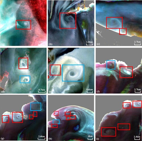
Submesoscale eddies are characterized by elliptical spiral patterns in remotely sensed images, which result from alterations in sea surface roughness due to tracer transport. By analyzing the rotational direction of these spiral patterns from the outer to inner regions, we can differentiate cyclonic eddies (CE) from anticyclonic eddies (AE), as illustrated in Figure 2. This rotational direction corresponds to the two types of eddy rotations observed in the Northern Hemisphere: CE rotates counterclockwise, while AE rotates clockwise (Chelton et al. 2011; Wang, Yang and Chen 2023; Zhang and Qiu 2020). It has also been observed that submesoscale eddies of different polarities exhibit symmetry within the same hemisphere.

Figure 2. (a)-(i) show submesoscale eddies on SDGSAT-1 images, where CE are indicated within red boxes and AE within blue boxes(in the northern hemisphere for example).

2.2. Problem formulations

To better elucidate the submesoscale eddy detection process, we have simplified it into a regression problem, inspired by the YOLO single-stage detection model. The input submesoscale eddy image is denoted as $X$. It is represented as a three-dimensional array $X\in R^{H\times W\times C}$, in which $H$ and $W$ represent the height and width of the image, while $C$ denotes the number of channels. The image is then divided into $N\times N$ grid cells, from which three parameters are predicted: the bounding box, confidence score, and class probability. These parameters collectively form the feature vector for each grid cell, which can be expressed as follows: (1) $Y=B\times (\mathrm{confidence},x,y,w,h,\mathrm{clas}{s}_{\mathrm{conditional}\mathrm{\_probability}})$(1) In the context of our analysis, $B$ denotes the number of predicted boxes, and $\mathrm{confidence}$ signifies whether the predicted boxes contain objects. The variables $x,y,w$ and $h$ indicate the center coordinates, width, and height of the predicted boxes obtained from the network's output. $\mathrm{clas}{s}_{\mathrm{conditional}\mathrm{\_probability}}$ denotes the conditional probability that the predicted boxes belong to each class. Consequently, this information allows for decoding the predicted boxes to derive their actual positions and dimensions.

To ensure high predictive accuracy, the model implements a loss function that quantifies the disparities between its predictions and the ground truth values. The loss function comprises three primary components: classification loss, confidence loss, and location loss, which are illustrated as follows: (2) $\mathrm{Loss}={\lambda }_1{L}_{\mathrm{loc}}+{\lambda }_2{L}_{\mathrm{cls}}+{\lambda }_3{L}_{\mathrm{conf}}$(2) In the presented framework, the balance coefficients ${\lambda }_1$, ${\lambda }_2$ and ${\lambda }_3$ are hyperparameters. $L_{\mathrm{loc}}$, $L_{\mathrm{cls}}$ and $L_{\mathrm{conf}}$ denote the location loss, classification loss, and confidence loss, respectively. $L_{\mathrm{loc}}$ and $L_{\mathrm{cls}}$ are computed for positive samples, whereas $L_{\mathrm{conf}}$ is calculated for all samples.

For $L_{\mathrm{loc}}$, we employ the Complete Intersection over Union (CIOU) loss introduced by Zheng et al. (2022). Unlike Distance Intersection over Union (DIOU) loss (Zheng et al. 2020), which considers the area of overlap and the distance between the centers of the predicted and ground truth boxes, CIOU loss also incorporates the aspect ratio of these boxes.

Additionally, both $L_{\mathrm{cls}}$ and $L_{\mathrm{conf}}$ are computed using Binary Cross-Entropy (BCE) loss. If $x$ denotes the predicted value and $x^{\mathrm{gt}}$ denotes the ground truth, then the equation is as follows: (3) $\mathrm{Loss}(x^{\mathrm{gt}},x)=x^{\mathrm{gt}}\log x+(1-x^{\mathrm{gt}})\log (1-x)$(3) $L_{\mathrm{cls}}$ reflects the classification performance of the model and is calculated as follows in Equation (4): (4) $L_{\mathrm{cls}}=\sum _{i=0}^{S\times S}\sum _{j=0}^B{\prod }_{\mathrm{ij}}^{\mathrm{obj}}\mathrm{Loss}(P_i^{\mathrm{gt}}(c),P_i(c))$(4) Where, $P_i(c)$ denotes the predicted probability when the prediction box recognizes the object as class $c$, while $P_i^{\mathrm{gt}}(c)$ denotes the label corresponding to the ground truth box.

In addition, $L_{\mathrm{conf}}$ quantifies the disparity in confidence between the predicted and ground truth boxes, and is expressed as follows: (5) $L_{\mathrm{conf}}=\sum _{i=0}^{S\times S}\sum _{j=0}^B{\prod }_{\mathrm{ij}}^{\mathrm{obj}}\mathrm{Loss}(C_i^{\mathrm{gt}},C_i)-\sum _{i=0}^{S\times S}\sum _{j=0}^B{\prod }_{\mathrm{ij}}^{\mathrm{noobj}}\mathrm{Loss}(C_i^{\mathrm{gt}},C_i)$(5) Where $C_i$ and $C_i^{\mathrm{gt}}$ denote the confidence of predicted box and ground truth box, respectively. In practice, if the $\mathrm{jth}$ bounding box of the $\mathrm{ith}$ grid cell predicts the object, the value of ${\prod }_{\mathrm{ij}}^{\mathrm{obj}}$is 1, and 0 otherwise. While ${\prod }_{\mathrm{ij}}^{\mathrm{noobj}}$is the converse of ${\prod }_{\mathrm{ij}}^{\mathrm{obj}}$.

As a result, by employing the above mathematical expressions, the localization and classification of eddies can be described more precisely.

3. Methodology

The YOLO (You Only Look Once) algorithm, introduced by Redmon in 2016, is a real-time object detection method trained on the MS COCO dataset to achieve cutting-edge performance. Unlike conventional object detection approaches that use classifiers, YOLO conceptualizes object detection as a regression problem, utilizing an end-to-end single network for detection (Redmon et al. 2016). This network processes raw images to produce bounding boxes and class labels for detected objects. In this study, we propose a multispectral eddy detection network (MEDNet), based on the improved YOLOv6 (Li et al. 2022), tailored for the precise detection of submesoscale eddies.

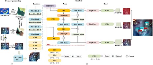
As depicted in Figure 3(b), the MEDNet architecture, following the design of YOLOv6, comprises three main components: the backbone, the neck, and the head. In multispectral imagery detection, input images often suffer degradation due to weak lighting in satellite imagery and cloud cover. Consequently, the image is subject to data enhancement and other preprocessing operations in the input section before entering the backbone network, as illustrated in Figure 3(a). To more effectively capture the spatial features of submesoscale eddies, an innovative multi-branch stacking block (MbS Block) has been incorporated into the backbone network. Simultaneously, the neck module performs feature fusion using a feature pyramid network (FPN) (Lin et al. 2017a) to further augment eddy features. Recognizing the diverse shapes and sizes of submesoscale eddies, the detection head utilizes multiple sub-heads, each designed to detect objects of varying sizes. This design facilitates the detection of eddies across various scales and shapes. Detailed insights into the various modules of MEDNet are provided in subsequent subsections.

Figure 3. Workflow of the MEDNet eddy detection technology. (a) shows the SDGSAT-1 multispectral data preprocessing flow, and (b) shows the MEDNet network architecture.

3.1. Pre-processing of multispectral eddy images

3.1.1. Linear stretching

In this study, a primary challenge in processing multispectral eddy images is their inconspicuous nature, attributed to poor contrast and brightness. To address these issues, we applied a linear stretching technique to the multispectral images to enhance their contrast. Linear stretching, a common image enhancement method in remote sensing, relies on pixel-wise linear transformations. This technique increases the contrast and brightness by mapping the minimum and maximum pixel values of the original data to a specified output range. The stretching equation is expressed as follows (Equation 6): (6) $g(x,y)={\displaystyle \frac{255}{(b-a)}\times (f(x,y)-a)}$(6) Where the original image $f(x,y)$ has a grey scale range of $[a,b]$ and the linearly stretched image has a greyscale range of $[0,255]$.

3.1.2. Multispectral eddy horizontal flip

The experimental methodology employs a cross-validation strategy where the SDG-Eddy 2022 dataset is randomly divided in a (9:1):1 ratio into training, validation, and test sets. Nevertheless, the imbalance in the quantity of CE (1389) and AE (602) in the remote sensing images results from factors like remote sensing technology, ocean dynamics, and seasonal variations. To mitigate this imbalance, we employed the Multispectral Eddy Horizontal Flip Technique (MEHFT).

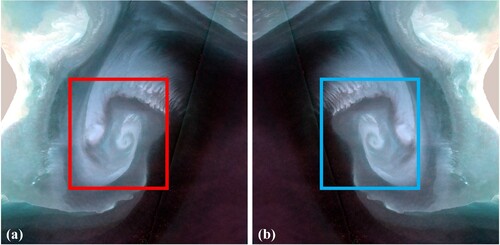
MEHFT primarily transforms the image along its vertical central axis. As discussed in Subsection 2.1, submesoscale eddy spiral curves with distinct polarities exhibit symmetry within the same hemisphere. Moreover, during the horizontal mirror flip, the processing of pixel information within each row remains consistent, and the order of rows is unaltered. Consequently, horizontally mirroring the original image (e.g. Figure 4(a)) along its central axis yields an eddy image with the opposite polarity (e.g. Figure 4(b)).

Figure 4. MEHFT on submesoscale eddy images. Where (a) is the image before processing and (b) is the image after processing.

This approach serves a dual purpose: it rectifies the imbalance between AE and CE ratios and augments the dataset, ensuring a sufficient supply of data for both model training and evaluation.

3.2. Backbone layer extraction features

The backbone network comprises a series of convolutional blocks (CBS), MbS blocks, and transition blocks. Each CBS block includes a convolutional layer, a batch normalization layer, and an activation function, specifically SiLU (Elfwing, Uchibe, and Doya 2018). Notably, the backbone feature extraction network exhibits two significant characteristics. First, it employs an innovative MbS block (Figure 5(a)) in place of the original RepBlock, and the internal residual block incorporates jump connections. Both the first and second branches modify channels using $1\times 1$ CBS modules. The third and fourth branches each utilize two $3\times 3$ CBS modules to extract eddy features, building on the work of the previous branches. By managing the shortest and longest path graduations, this module enables the network to acquire additional characteristics and enhance its robust performance. Second, an innovative oversampling module replaces the traditional $3\times 3$ convolution kernel downsampling technique, which used a step size of two. Figure 5(b) illustrates this approach, integrating two commonly used transition modules for downsampling: one with a convolution kernel size of $3\times 3$ and a step size of $2\times 2$, and another using maximum pooling with a $2\times 2$ stride. Each transition module branches into two paths. The left path comprises maximum pooling with a $2\times 2$ stride, followed by a $1\times 1$ CBS module. The right path includes a $1\times 1$ CBS module and another $3\times 3$ CBS module with a stride size of 2. The outputs of these paths are then concatenated. Specifically, the maxpooling layer significantly enlarges the receptive field of the current feature layer. This enlarged feature layer is subsequently fused with features processed by standard convolution. As a result, this fusion enhances the network's generalization capabilities.

Figure 5. Structure of each module. (a) MbS Block. (b) Transition Block. (c) SPPCSPC.

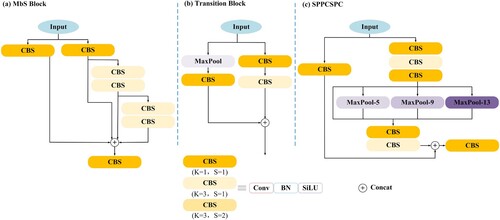
3.3. Neck layer multi-scale fusion

Neck structures include the SPPCSPC structure, which combines spatial pyramid pooling (SPP) (He et al. 2015) with cross stage partial channel (CSPC), as well as the FPN structure. The SPPCSPC structure divides features into two parts, as shown in Figure 5(c). The left branch undergoes conventional convolution operations, while the right branch applies maximum pooling at four different scales (sizes of 1, 5, 9, 13 respectively) to differentiate between large and small objects. This combination of branches reduces computational demands by half, thus accelerating and enhancing the accuracy of model training. MEDNet's FPN, an enhanced feature extraction network, fuses feature layers of various forms to more effectively extract eddy features. Specific details of the FPN are highlighted in the red boxed line in Figure 3(b). A key advantage of this neck network design is its effective resolution of the multi-scale feature fusion challenge, thereby improving the performance and efficiency of submesoscale eddy detection.

3.4. Detection output head

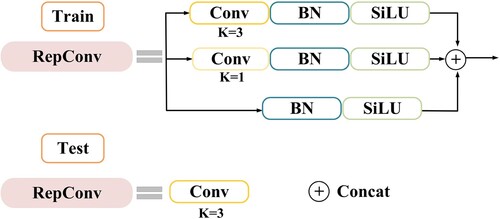
Before transitioning to head prediction, we utilize a RepConv structure, inspired by RepVGG (Ding et al. 2021). The fundamental concept involves introducing specialized residual structures to aid in training, while simplifying these complex structures to function as ordinary convolutional layers during testing, as illustrated in Figure 6. This approach simplifies the network architecture without compromising its predictive performance. This module produces three distinct scales of feature layers: (20, 20, 21), (40, 40, 21), and (80, 80, 21). Each scale of feature layer is responsible for detecting eddies of varying sizes, with the larger-scale layers specifically targeting smaller-scale eddies, attributed to their smaller receptive fields.

Figure 6. Structure of RepConv.

The final dimension of these feature layers represents seven parameters corresponding to the three a priori frames: prediction box position $(x,y)$, width ($w$), height ($h$), confidence, and category probabilities. By decoding the prediction results from these three feature layers, we obtain the ultimate prediction outcomes. Subsequently, these results are subjected to score ranking and non-maximum suppression (NMS) (Neubeck and Van Gool 2006) to generate the final prediction boxes.

4. Experiments and results

4.1. Implementation details and Quantitative evaluation

The experiments utilized PyTorch, with models trained for up to 300 epochs on an NVIDIA RTX A6000 GPU. During training, we used an adaptive moment estimation (Adam) optimizer with a cosine decay learning rate scheduling strategy, starting at an initial learning rate of 0.01. Additionally, to expedite model convergence and minimize memory consumption, weight decay was set to zero and the momentum parameter was established at 0.937.

To validate the eddy detection results, we employed the VOC (Visual Object Classes) metric, officially used for verification in the DOTA (Detection and Tracking in Aerial Imagery) dataset (Everingham et al. 2010). These metrics include the F1 score, average precision (AP), and mean Average Precision (mAP) at an Intersection over Union (IoU) threshold of 0.5. Model prediction results were also assessed using precision and recall. Accuracy is defined as the ratio of correctly predicted positive samples (submesoscale eddies) to all samples predicted as positive by the model. Recall is represented as the ratio of correctly predicted positive samples to all actual positive samples.

4.2. Comparison of experimental results with other models

Upon completion of model training, we selected 222 images from the test set for evaluation. Table 1 presents an overview of the evaluation metrics used to detect different polarities of eddies with MEDNet on the SDG-Eddy 2022 dataset. The data in Table 1 clearly shows that our model achieves remarkable accuracy and recall in eddy detection. Notably, the model exhibits outstanding detection performance for anticyclonic eddies (AE), achieving precision, recall, and F1 scores of 92.68%, 90.48%, and 94.00%, respectively.

Table 1. Precision, recall, F1-score of MEDNet on the SDG-Eddy 2022 dataset.

Method	Precision (%)		Recall (%)		F1 score (%)
	AE	CE	AE	CE	AE	CE
MEDNet	92.68	88.15	90.48	81.67	94.00	87.00

To comprehensively demonstrate MEDNet's performance in eddy detection, this study conducted a comparative analysis with other object detection models such as SSD (Liu et al. 2016), RetinaNet (Lin et al. 2017b), YOLOv3 (Redmon and Farhadi 2018), YOLOv4 (Bochkovskiy, Wang, and Liao 2020), YOLOv5s, DETR (Carion et al. 2020), EfficientDet (Tan, Pang, and Le 2020), YOLOv7x (Wang, Bochkovskiy and Liao 2023) and YOLOv8, using the SDG-Eddy 2022 dataset. Both quantitative and qualitative comparisons were used to assess the performance of these networks. Notably, consistent training hyperparameters were maintained throughout the evaluation to align with those used for MEDNet.

Quantitatively, Table 2 presents the comparative results of all models, detailing AP and mAP at a confidence threshold of 0.5. The results in Table 2 clearly demonstrate that our method outperforms all others in both metrics. Notably, MEDNet achieved an mAP of 90.42% in eddy detection. Compared to SSD, RetinaNet, YOLOv3, YOLOv4, YOLOv5s, DETR, EfficientDet, YOLOv7x, YOLOv8s and YOLOv8n, MEDNet showed performance improvements of 46.37%, 9.54%, 28.04%, 17.51%, 3.63%, 20.05%, 29.68%, 2.64%, 18.75% and 16.31%,respectively.

Table 2. Comparison with the different networks in AP and mAP0.5.

Methods	AP (%)		mAP0.5(%)
	AE	CE
SSD	42.19	45.91	44.05
RetinaNet	78.68	83.07	80.88
YOLOv3	57.37	67.38	62.38
YOLOv4	77.82	67.99	72.91
YOLOv5s	84.13	89.45	86.79
DETR	69.08	71.66	70.37
EfficientDet	59.70	61.79	60.74
YOLOV7x	87.34	88.22	87.78
YOLOV8s	77.92	67.43	71.67
YOLOV8n	72.93	75.30	74.11
MEDNet	92.68	88.15	90.42

Moreover, Figure 7 presents a qualitative analysis that visually compares the detection results from various network models across four representative images. Blue boxes represent anticyclonic eddies (AE), and red boxes indicate cyclonic eddies (CE). Each prediction box displays the predicted class along with the confidence information. These visual presentations underscore the model’s sensitivity to the complexities of oceanic environments and the variability in satellite imagery quality.

Figure 7. Image identification results of eddies on SDG-Eddy 2022. (a) Ground truths. (b) YOLOv3, (c) SSD, (d) RetinaNet, and (e) MEDNet.

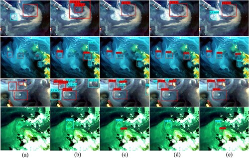
The first row showcases how various models detect eddies resulting from the interaction between artificial structures and marine dynamics. The second and third rows demonstrate the model's capability to identify eddies resulting from the complex interactions of islands with flow fields in shallow coastal regions. The fourth row illustrates the model’s proficiency in detecting eddies in images characterized by significant cloud cover. Comparative analysis indicates that MEDNet excels at detecting eddies across various scales and environmental conditions, outperforming other models, particularly in reducing omission errors associated with smaller-scale eddies. Specifically, in the third row, other models exhibit false positives for AE, while MEDNet consistently achieves precise detections with high confidence levels. The key emphasis is on the strong correlation between our model's detection results and the ground truth, highlighting its capability to accurately differentiate between eddies of various scales.

4.3. Visualisation of feature maps

To provide a more detailed demonstration of MEDNet's operation on the SDG-Eddy 2022 dataset, features at various locations within MEDNet were visualized using Grad-CAM (Selvaraju et al. 2017). Specifically, heatmap visual analyses were conducted on the SPPCSPC module and the three head layers, as depicted in Figure 8.

Figure 8. Visualizing chosen feature maps at distinct positions within the proposed MEDNet. (a) represents the original image for detection, while (b)-(f) respectively illustrate the visualized heatmaps of feature layers outputted by the backbone network, SPPCSPC module, and three head layers out.

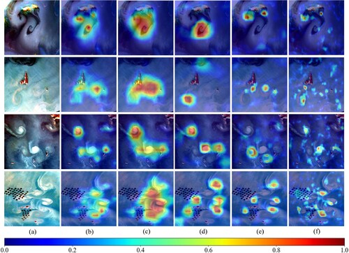
In Figure 8, panel (a) shows the original image used for detection, while panels (b) through (f) illustrate the visualized heatmaps of feature layers from the backbone network, the SPPCSPC module, and the three head layers. The impact of the SPPCSPC module is evident, as it uniformly distributes the network's attention across both the centers and edges of eddies, following processing by the backbone network. Additionally, the SPPCSPC module demonstrates robustness in preserving target integrity and in the detection of smaller targets. With its assistance, our model effectively detects smaller-scale eddies, which are prone to being overlooked, and accurately identifies medium to large-scale eddies. Furthermore, panels 8(d), 8(e), and 8(f) display the detection capabilities of the small-scale, medium-scale, and large-scale feature layers, respectively, showcasing their effectiveness in identifying eddies of various sizes. Observations from Figure 8 reveal that the small-scale feature layer primarily focuses on capturing larger-scale eddies and exhibits a significant advantage in detecting the completeness of these eddies. The large-scale feature layer specializes in detecting smaller-scale eddies, whereas the medium-scale layer enhances detection of intermediate-sized eddies. It should be noted that while different-scale feature layers may detect the same eddy, the final prediction box responsible for detection must undergo score ranking and NMS filtering to yield the ultimate result. In summary, these visualizations underscore the effectiveness of key modules within our model, demonstrating its robustness and outstanding performance in capturing eddy features across various scales.

4.4. Ablation study

To ascertain the efficacy of the SPPCSPC and MbS Block, we conducted ablation experiments on the SDG-Eddy 2022 dataset. AP and mAP have been chosen as metrics for evaluating the effect of different components of the model. Table 3 presents the quantitative model performances on the SDG-Eddy 2022 dataset in detail, after the removal of different module groups. The findings reveal that the elimination of different modules exerts varying degrees of influence on the model's performance. The baseline model, formed by concurrently excluding the SPPCSPC and MbS Block, achieved a mAP of 87.25%. Thereafter, we systematically introduced the SPPCSPC and MbS Block into the baseline model, observing their respective effects.

Table 3. Robustness Testing on SDG-Eddy 2022 dataset.

Base model	SPPCSPC	MbS Block	AP (%)		mAP (%)
			AE	CE
√			89.75	84.74	87.25
√	√		90.08	88.57	89.33
√		√	91.09	86.25	88.72
√	√	√	92.68	88.15	90.42

Overall, the incorporation of the SPPCSPC module resulted in a significant increase of 2.08% in mAP. Moreover, this module also achieved the highest average precision (AP) for cyclonic eddies (CE). Similarly, introducing the MbS Block resulted in a 1.47% improvement in the baseline mAP, while also achieving the highest AP for anticyclonic eddies (AE). The data in the final row demonstrate that integrating all modules into the baseline network maximizes detection performance, yielding APs of 92.68% for AE and 88.15% for CE. Furthermore, the mean Average Precision (mAP) significantly increased to 90.42%. These results unequivocally demonstrate that including the SPPCSPC and MbS Block substantially enhances the model’s ability to detect eddies across various categories.

4.5. Characteristics of detected eddies

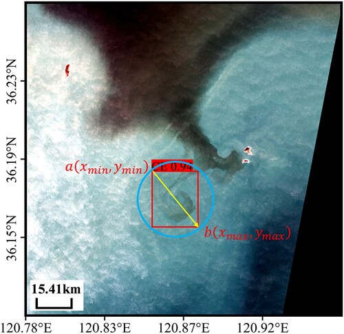
In this section, the East China Sea (ECS) serves as the study area for characterizing the 712 oceanic eddies identified within this region. The edge of an eddy is defined as its outermost spiral, and the eddy’s position is determined by the bounding box formed around the eddy’s boundary. Specifically, by considering the radius of the bounding box’s outer circle as the eddy's radius and approximating the bounding box’s area as that of its outer circle, the radius of the eddy can be estimated as follows: (7) $R=\sqrt{{\displaystyle \frac{(x_{max}-x_{min})\times (y_{max}-y_{min})}{\pi }}}\times 10$(7) Where the maximum and minimum coordinates of the vertices of the eddy bounding box are denoted as $(x_{min},y_{min})$ and $(x_{max},y_{max})$, respectively. 10 denotes the satellite resolution in metres (schematic shown in Figure 9). The purpose of this definition and calculation method is to provide a clear and practical description of eddy boundaries, facilitating the accurate determination of eddy characteristics for further analysis. This method efficiently captures the geometric shapes of eddies, providing valuable insights for the study of their characteristics.

Figure 9. Schematic diagram of the detected eddy radius calculation. The red box indicates the prediction bounding box (a and b are the coordinates of the upper-left and lower-right corners of the prediction box, respectively), the blue circle indicates the eddy boundary, and the yellow line indicates the eddy diameter.

Using the definitions provided, we conducted detailed measurements and statistical analyses of oceanic eddy sizes in the study area, as illustrated in Figure 10. Overall, most eddies in the ECS have radii smaller than 5 km, comprising 94% of the total observed. According to McWilliams (2016), the radius of submesoscale eddies is smaller than the first baroclinic Rossby radius of deformation and larger than the thickness of the turbulent mixing layer in the areas where they are located. According to Chelton et al. (1998), the radius of the first oblique pressure Rossby waves in the ECS generally ranges from 20 km to 50 km. Therefore, it can be concluded that the eddies observed by SDGSAT-1 in the ECS are predominantly submesoscale.

Figure 10. A frequency plot displaying the distribution of radii for CE and AE in the ECS.

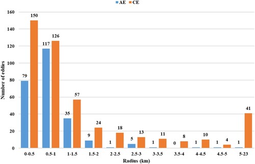
Additionally, the radii of both CE and AE are primarily distributed within the 0-1.5 km range. Within the 0-0.5 km range, CE occur most frequently, whereas in the 0.5-1.0 km range, AE are numerous but less frequent than CE. Almost all AE radii fall within the 0–2 km range, whereas CE radii show a broader distribution. This suggests that CE generally have larger scales compared to AE, with 41 eddies having radii exceeding 5 km.

It should be noted that SDGSAT-1 detected significantly more CE (462) than AE (250) besides the characteristics of the eddy radius. This disparity is mainly attributed to the high Rossby number in the ECS, which weakens the centrifugal instability of AE, while CE maintain greater coherence (Dong, McWilliams, and Shchepetkin 2007). Consequently, the detection results reveal a significantly higher quantity of CE compared to AE.

4.6. Validation and comparison with SST and Chl-a data

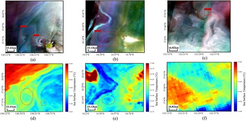
The spiral structure of eddies significantly affects the state of seawater at the surface. Cyclonic eddies (CE) disperse sea surface water under the effect of geostrophic rotation, causing the lower layer of seawater to rise, resulting in lower SST inside the eddy compared to the surrounding seawater – a negative temperature anomaly. Conversely, anticyclonic eddies (AE) converge sea surface water, causing the upper layer to sink, which results in higher SST – a positive temperature anomaly. Simultaneously, as the nutrients from the lower layers rise with the seawater in CE, Chl-a concentration increases, showing a positive anomaly. In AE, nutrients sink with the surface layer, decreasing the Chl-a concentration and showing a negative anomaly. To validate the detected eddies, SST data from Sentinel 3 (1000 m spatial resolution) and sea surface Chl-a concentration data from GOCI2 (250 m spatial resolution) were used for comparison with observations from SDGSAT-1.

Both Sentinel 3A and Sentinel 3B satellites currently operate in sun-synchronous orbits. The Sea and Land Surface Temperature Radiometer (SLSTR), a dual-view scanning thermo-radiometer, operates in a near-Earth orbit at an altitude of 800–830 kilometers. With a spatial resolution of 1000 m, it covers global sea and land surface temperatures, providing valuable data for climate and meteorological studies (Coppo, Smith, and Nieke 2015). SST anomalies due to oceanic eddies were validated using Level 2 SST data from Sentinel 3, provided by EUMETSAT.

We selected three sets of images from SDGSAT-1 for comparative experiments. Figure 11(a-c) display the eddy detection results from SDGSAT-1 images, while Figures 11(d-f) show the corresponding SST data from Sentinel 3 during the same period. As depicted in the figures, the cyclonic eddies (CEs) detected in the SDGSAT-1 images correspond to regions in the Sentinel 3 data that exhibit lower SST at the center compared to the surrounding areas, aligning with the typical SST distribution pattern of CEs. This alignment verifies the accuracy of our model's eddy detection to some extent.

Figure 11. Comparison of results with SST. (a–c) shows the detection results of eddies in SDGSAT-1, (d–f) Sentinel-3 SST data.

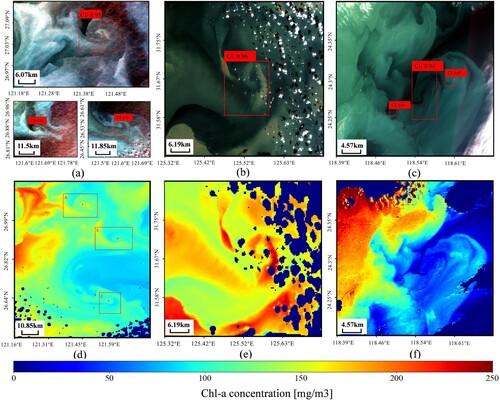
GOCI is an oceanic sensor aboard the Korean satellite COMS (Communication, Ocean, and Meteorological Satellite). As the world's first geostationary ocean remote sensing satellite, GOCI features eight spectral bands, including those necessary for visible light and estimating Chl-a fluorescence (Ryu et al. 2012). Launched in February 2020, GOCI2, the successor to GOCI, offers a 250 m spatial resolution, up to 13 spectral bands, and can generate data from up to 10 views daily. In this study, we used GOCI2 Chl-a data to validate anomalies in Chl-a concentrations resulting from oceanic eddies.

We selected three sets of images from the ECS, captured by SDGSAT-1, for the comparison experiments. Figure 12(a-c) display the detection results of eddies from SDGSAT-1 images, while Figure 12(d-f) illustrate the corresponding Chl-a concentrations from GOCI2. In all three experiments, the eddies detected in the SDGSAT-1 images correspond closely with those identified in the GOCI2 regions. Smaller-scale eddies did not correspond to higher Chl-a concentrations in GOCI2 images, likely influenced by surrounding regions with elevated Chl-a levels (as shown in Figure 12(d,f)). However, larger-scale eddies showed higher Chl-a concentrations in GOCI2 data (Figure 12(e)). Thus, the GOCI2 Chl-a data confirm the SDGSAT-1 observations of eddies. The first set of comparisons demonstrates that SDGSAT-1, with its higher resolution, clearly reveals the spiral structures of eddies, indicating superior mapping quality compared to GOCI2. Additionally, the third set of comparisons reveals that GOCI2, due to its limited spatial resolution, fails to detect submesoscale eddies smaller than 2 km in diameter that are detected by SDGSAT-1 (as seen in the lower left of Figure 12(c)). This further indicates that SDGSAT-1 high-resolution satellite images are capable of detecting small-scale eddies that may not be recognized by medium resolution images.

Figure 12. Comparison of results with Chl-a. (a–c) shows the detection results of eddies in SDGSAT-1, (d–f) GOCI2 Chl-a data.

5. Conclusion

The study of submesoscale oceanic eddies, unlike mesoscale ones, requires higher satellite resolution. High-resolution multispectral data provide detailed and accurate information that aids in the precise localization of eddies, offering a new data source for submesoscale eddy research. However, the advantages of high-resolution multispectral data have largely been overlooked. This study introduces MEDNet, a submesoscale eddy detection model based on high-resolution multispectral images from SDGSAT-1. Experimental results show that MEDNet outperforms other detection methods, achieving a mean average precision (mAP) of up to 90.42%. Additionally, the eddies detected by SDGSAT-1 align with SST and Chl-a concentration data. A negative SST anomaly and a positive Chl-a anomaly were observed in the cyclonic eddies, consistent with earlier studies. Furthermore, high-resolution multispectral data facilitate the detection of more eddies by providing finer spatial information, enabling more accurate detection of small-scale eddy structures. However, this study is not without limitations. As mentioned earlier, multispectral data allow for the observation of oceanic eddies through tracers like suspended sediment; however, tracer concentrations vary regionally. In coastal areas, significant changes in tracer concentrations at the sea surface facilitate the observation of submesoscale oceanic eddies by satellite sensors. In contrast, in deep-sea areas with small tracer concentration gradients, observable eddy information is limited. To mitigate these limitations, an image enhancement algorithm was employed to improve eddy feature detection in areas with lower tracer concentrations. While the SDG-Eddy 2022 dataset includes 1,991 submesoscale eddies, providing a substantial volume of high-resolution multispectral data, further expansion is necessary as the data is updated. Therefore, future research should focus on the timely expansion of the submesoscale eddy dataset to enrich the data available for oceanographic research.

Disclosure statement

No potential conflict of interest was reported by the author(s).

Data availability statement

Data in support of this study were provided by the International Research Centre of Big Data for Sustainable Development Goals. (http://124.16.184.48:6008/home).

Additional information

Funding

This work was jointly supported by Laoshan Laboratory science and technology innovation projects (LSKJ202201406, LSKJ202201302), National Natural Science Foundation of China (42276203), Natural Science Foundation of Shandong Province (ZR2021MD001).

References

- Becker, Fernando, S. I. Romero, and J. P. Pisoni. 2023. “Detection and Characterization of Submesoscale Eddies from Optical Images: A Case Study in the Argentine Continental Shelf.” International Journal of Remote Sensing 44 (10): 3146–3159. https://doi.org/10.1080/01431161.2023.2216853.
- Bochkovskiy, A., C. Wang, and H. M. Liao. 2020. “Yolov4: Optimal Speed and Accuracy of Object Detection.” arXiv. https://doi.org/10.48550/arXiv.2004.10934.
- Capet, X., J. C. McWilliams, M. J. Molemaker, and A. F. Shchepetkin. 2008. “Mesoscale to Submesoscale Transition in the California Current System. Part I: Flow Structure, Eddy Flux, and Observational Tests.” Journal of Physical Oceanography 38 (1): 29–43. https://doi.org/10.1175/2007JPO3671.1.
- Carion, N., F. Massa, G. Synnaeve, N. Usunier, A. Kirillov, and S. Zagoruyko. 2020. “End-to-end Object Detection with Transformers.” In European Conference on Computer vision(ECCV12346. 213–229. Cham: Springer International Publishing. https://doi.org/10.1007/978-3-030-58452-8_13.
- Chelton, D. B., R. A. DeSzoeke, M. G. Schlax, K. E. Naggar, and N. Siwertz. 1998. “Geographical Variability of the First Baroclinic Rossby Radius of Deformation.” Journal of Physical Oceanography 28 (3): 433–460. https://doi.org/10.1175/1520-0485(1998)028<0433:GVOTFB>2.0.CO;2.
- Chelton, D. B., P. Gaube, M. G. Schlax, J. J. Early, and R. M. Samelson. 2011. “The Influence of Nonlinear Mesoscale Eddies on Near-Surface Oceanic Chlorophyll.” Science 334 (6054): 328–332. https://doi.org/10.1126/science.1208897.
- Cheng, X. H., Q. Y. Quan, and W. W. Qiang. 2005. “Seasonal and Interannual Variabilities of Mesoscale Eddies in South China Sea.” Acta Pharmacologica Sinica 26 (4): 1387–1394. https://doi.org/10.1111/j.1745-7254.2005.00209.x.
- Coppo, P., D. Smith, and J. Nieke. 2015. “Sea and Land Surface Temperature Radiometer on Sentinel-3.” Optical Payloads for Space Missions 701–714. https://doi.org/10.1002/9781118945179.ch32.
- Ding, X., X. Zhang, N. Ma, J. Han, G. Ding, and J. Sun. 2021. “Repvgg: Making vgg-Style Convnets Great Again.” In Proceedings of the IEEE/CVF Conference on Computer Vision and Pattern Recognition(CVPR), Nashville, TN, USA. 13728–13737. IEEE. https://doi.org/10.1109/CVPR46437.2021.01352.
- Dong, C., J. C. McWilliams, and A. F. Shchepetkin. 2007. “Island Wakes in Deep Water.” Journal of Physical Oceanography 37 (4): 962–981. https://doi.org/10.1175/JPO3047.1.
- Elfwing, S., E. Uchibe, and K. Doya. 2018. “Sigmoid-weighted Linear Units for Neural Network Function Approximation in Reinforcement Learning.” Neural Networks 107:3–11. https://doi.org/10.1016/j.neunet.2017.12.012.
- Everingham, M., L. Van Gool, C. Williams, J. Winn, and A. Zisserman. 2010. “The Pascal Visual Object Classes (voc) Challenge.” International Journal of Computer Vision 88:303–338. https://doi.org/10.1007/s11263-009-0275-4.
- Frenger, I., N. Gruber, R. Knutti, and M. Münnich. 2013. “Imprint of Southern Ocean Eddies on Winds, Clouds and Rainfall.” Nature Geoscience 6 (8): 608–612. https://doi.org/10.1038/ngeo1863.
- Ge, L., B. Huang, X. Chen, and G. Chen. 2023. “Medium-range Trajectory Prediction Network Compliant to Physical Constraint for Oceanic Eddy.” IEEE Transactions on Geoscience and Remote Sensing 61:1–14. https://doi.org/10.1109/TGRS.2023.3298020.
- Guo, H., C. Dou, H. Chen, J. Liu, B. Fu, X. Li, Z. Zou, and D. Liang. 2023. “SDGSAT-1: The World’s First Scientific Satellite for Sustainable Development Goals.” Science Bulletin 68 (1): 34–38. https://doi.org/10.1016/j.scib.2022.12.014.
- He, K., X. Zhang, S. Ren, and J. Sun. 2015. “Spatial Pyramid Pooling in Deep Convolutional Networks for Visual Recognition.” IEEE Transactions on Pattern Analysis and Machine Intelligence 37 (9): 1904–1916. https://doi.org/10.1109/TPAMI.2015.2389824.
- Ji, Y., G. Xu, C. Dong, J. Yang, and C. Xia. 2021. “Submesoscale Eddies in the East China Sea Detected from SAR Images.” Acta Oceanologica Sinica 40 (3): 18–26. https://doi.org/10.1007/s13131-021-1714-5.
- Karimova, S. 2012. “Spiral Eddies in the Baltic, Black and Caspian Seas as Seen by Satellite Radar Data.” Advances in Space Research 50 (8): 1107–1124. https://doi.org/10.1016/j.asr.2011.10.027.
- Karimova, S., and M. Gade. 2016. “Improved Statistics of Sub-Mesoscale Eddies in the Baltic Sea Retrieved from SAR Imagery.” International Journal of Remote Sensing 37 (10): 2394–2414. https://doi.org/10.1080/01431161.2016.1145367.
- Li, C., L. Li, H. Jiang, K. Weng, Y. Geng, L. Li, Z. Ke, et al. 2022. “YOLOv6: A Single-Stage Object Detection Framework for Industrial Applications.” arXiv abs/2209.02976. https://doi.org/10.48550/arXiv.2209.02976.
- Lin, T.-Y, P. Dollár, R. Girshick, K. He, B. Hariharan, and S. Belongie. 2017a. “Feature Pyramid Networks for Object Detection.” In Proceedings of the IEEE Conference on Computer Vision and Pattern Recognition(CVPR), Honolulu, HI, USA. 936–944. IEEE. https://doi.org/10.1109/CVPR.2017.106.
- Lin, T.-Y., P. Goyal, R. Girshick, K. He, and P. Dollár. 2017b. “Focal Loss for Dense Object Detection.” In Proceedings of the IEEE International Conference on Computer Vision(ICCV), Venice, Italy. 2999–3007. IEEE. https://doi.org/10.1109/ICCV.2017.324.
- Liu, W., D. Anguelov, D. Erhan, C. Szegedy, S. Reed, C. Fu, and A. C. Berg. 2016. “Ssd: Single Shot Multibox Detector.” In Computer Vision–ECCV 2016: 14th European Conference, Amsterdam, The Netherlands. 21–37. Springer International Publishing. https://doi.org/10.1007/978-3-319-46448-0_2.
- McWilliams, J. C. 2016. “Submesoscale Currents in the Ocean.” Proceedings of the Royal Society A: Mathematical, Physical and Engineering Sciences 472 (2189): 20160117. https://doi.org/10.1098/rspa.2016.0117.
- McWilliams, J. C. 2019. “A Survey of Submesoscale Currents.” Geoscience Letters 6 (1): 3. https://doi.org/10.1186/s40562-019-0133-3.
- Neubeck, A., and L. Van Gool. 2006. “Efficient non-Maximum Suppression.” In 18th International Conference on Pattern Recognition (ICPR'06), Hong Kong, China. vol. 3, 850–855. IEEE. https://doi.org/10.1109/ICPR.2006.479.
- Ni, Q., X. Zhai, C. Wilson, C. Chen, and D. Chen. 2021. “Submesoscale Eddies in the South China Sea.” Geophysical Research Letters 48 (6): e2020. https://doi.org/10.1029/2020GL091555.
- Qin, L. J., Q. Dong, X. Fan, C. J. Xue, X. Y. Hou, and W. J. Song. 2015. “Temporal and Spatial Characteristics of Mesoscale Eddies in the North Pacific Based on Satellite Altimeter Data.” National Remote Sensing Bulletin 19 (5): 806–817. https://doi.org/10.11834/jrs.20154154.
- Redmon, J., S. Divvala, R. Girshick, and A. Farhadi. 2016. “You Only Look Once: Unified, Real-Time Object Detection.” Proceedings of the IEEE Conference on Computer Vision and Pattern Recognition 779–788. https://doi.org/10.1109/CVPR.2016.91.
- Redmon, J., and A. Farhadi. 2018. “Yolov3: An Incremental Improvement.” arXiv abs/1804.02767. https://doi.org/10.48550/arXiv.1804.02767.
- Ryu, J. H., H. J. Han, S. Cho, Y. J. Park, and Y. H. Ahn. 2012. “Overview of Geostationary Ocean Color Imager (GOCI) and GOCI Data Processing System (GDPS).” Ocean Science Journal 47 (3): 223–233. https://doi.org/10.1007/s12601-012-0024-4.
- Selvaraju, R. R., M. Cogswell, A. Das, R. Vedantam, D. Parikh, and D. Batra. 2017. “Grad-Cam: Visual Explanations from Deep Networks via Gradient-Based Localization.” In Proceedings of the IEEE International Conference on Computer Vision(ICCV), Venice, Italy. 618–626. IEEE. https://doi.org/10.1109/ICCV.2017.74.
- Tan, M., R. Pang, and Q. V. Le. 2020. “Efficientdet: Scalable and Efficient Object Detection.” In Proceedings of the IEEE/CVF Conference on Computer Vision and Pattern Recognition(CVPR), Seattle, WA, USA. 10778–10787. IEEE. https://doi.org/10.1109/CVPR42600.2020.01079.
- Taylor, J. R., and A. F. Thompson. 2023. “Submesoscale Dynamics in the Upper Ocean.” Annual Review of Fluid Mechanics 55:103–127. https://doi.org/10.1146/annurev-fluid-031422-095147.
- Vincent, G., K. Pak, D. Martinez, E. Goh, J. Wang, B. Bue, B. Holt, and B. Wilson. 2023. “Unsupervised SAR Images for Submesoscale Oceanic Eddy Detection.” In IGARSS 2023-2023 IEEE International Geoscience and Remote Sensing Symposium, Pasadena, CA, USA. 2065-2068. IEEE. https://doi.org/10.1109/IGARSS52108.2023.10282488.
- Wang, C.-Y., A. Bochkovskiy, and H.-Y. M. Liao. 2023. “YOLOv7: Trainable bag-of-Freebies Sets new State-of-the-art for Real-Time Object Detectors.” In Proceedings of the IEEE/CVF Conference on Computer Vision and Pattern Recognition(CVPR), Vancouver, BC, Canada. 7464–7475. IEEE. https://doi.org/10.1109/CVPR52729.2023.00721.
- Wang, Y., and J. Chong. 2020. “Detection Method of Oceanic Eddies Using Tiangong-2 Near-Nadir Interferometric SAR.” National Remote Sensing Bulletin 24 (9): 1070–1076. https://doi.org/10.11834/jrs.20209231.
- Wang, Y., J. Yang, and G. Chen. 2023. “Euphotic Zone Depth Anomaly in Global Mesoscale Eddies by Multi-Mission Fusion Data.” Remote Sensing 15 (4): 1062. https://doi.org/10.3390/rs15041062.
- Xia, L., G. Chen, X. Chen, L. Ge, and B. Huang. 2022. “Submesoscale Oceanic Eddy Detection in SAR Images Using Context and Edge Association Network.” Frontiers in Marine Science 9:1023624. https://doi.org/10.3389/fmars.2022.1023624.
- Xu, G., J. Yang, C. Dong, D. Chen, and J. Wang. 2015. “Statistical Study of Submesoscale Eddies Identified from Synthetic Aperture Radar Images in the Luzon Strait and Adjacent Seas.” International Journal of Remote Sensing 36 (18): 4621–4631. https://doi.org/10.1080/01431161.2015.1084431.
- Zhang, D., M. Gade, W. Wang, and H. Zhou. 2023. “EddyDet: A Deep Framework for Oceanic Eddy Detection in Synthetic Aperture Radar Images.” Remote Sensing 15 (19): 4752. https://doi.org/10.3390/rs15194752.
- Zhang, Z., and B. Qiu. 2020. “Surface chlorophyll enhancement in mesoscale eddies by submesoscale spiral bands.” Geophysical Research Letters 47 (14): e2020GL088820. https://doi.org/10.1029/2020GL088820.
- Zhang, J., S. Wang, S. Zhang, F. Tang, W. Fan, S. Yang, Y. Sun, et al. 2022. “Research on Target Detection of Engraulis Japonicus Purse Seine Based on Improved Model of YOLOv5.” Frontiers in Marine Science 9:933735. https://doi.org/10.3389/fmars.2022.933735.
- Zheng, Z., P. Wang, W. Liu, J. Li, R. Ye, and D. Ren. 2020. “Distance-IoU Loss: Faster and Better Learning for Bounding box Regression.” Proceedings of the AAAI Conference on Artificial Intelligence 34 (07): 12993–13000. https://doi.org/10.1609/aaai.v34i07.6999.
- Zheng, Z., P. Wang, D. Ren, W.Liu, R. Ye, Q. Hu, and W. Zuo. 2022. “Enhancing Geometric Factors in Model Learning and Inference for Object Detection and Instance Segmentation.” IEEE Transactions on Cybernetics 52 (8): 8574–8586. https://doi.org/10.1109/TCYB.2021.3095305.