Predicting time series of vegetation leaf area index across North America based on climate variables for land surface modeling using attention-enhanced LSTM

ABSTRACT

Ecosystem process modeling is vital for a broad range of applications. It requires a key metric to characterize vegetation canopies: the leaf area index (LAI). Many land surface models utilize satellite-derived LAI for modeling ecosystem processes. The use of satellite-derived LAI constrains the models for predicting ecosystem processes when observational data are unavailable. Enriching prognostic models for predicting the LAI is favorable to land surface studies for forecasting vegetation-related processes. An attention-enhanced long and short memory (AELSTM) model was developed to predict the vegetation LAI time series based on climatic data. The AELSTM outperformed comparative machine learning models when assessed using satellite and flux tower data. The LAI predicted by AELSTM are temporally and spatially consistent with satellite-derived LAI. The R² values attained 0.86–0.93 across biomes. AELSTM can be coupled with the land surface models to predict gross primary productivity. Our proposed model was demonstrated to be effective in predicting the LAI time series under different Shared Socioeconomic Pathways in CMIP6. Our study demonstrated that deep learning approaches are capable of modeling and characterizing the spatial and temporal patterns of key vegetation variables such as LAI. Moreover, the study has provided references for vegetation processes in land surface studies.

HIGHLIGHTS

• A deep learning model to predict the time series of LAI for land surface modeling.

• Predicted LAI exhibits spatio-temporal consistency with satellite-derived LAI.

• The model can be coupled with a land surface model to enable GPP prediction.

• The predicted LAI is consistent with the LAI in future scenarios from CMIP6.

KEYWORDS:

• Vegetation
• deep learning
• land surface model
• time series prediction
• meteorology

1. Introduction

Terrestrial vegetation plays a crucial role in the biosphere. It influences the carbon and water cycles of the land surface. The observable characteristics of plant leaves, such as the area and color variations, are indicative of vegetation growth and reflect the global climate and environmental impacts on terrestrial ecosystems (Verger et al. 2016). The leaf area index (LAI) represents the total leaf area per unit land area. It serves as a core metric that quantifies the amount of plant leaf variation on the land surface. Terrestrial ecosystem models widely use the LAI to characterize vegetation canopies while simulating ecosystem processes. The LAI largely determines the performance of terrestrial ecosystem models in simulating a series of ecological processes such as radiative transfer, respiration, photosynthesis, and evapotranspiration (Chen et al. 2016).

Current LAI modeling methods for land surface studies include diagnostic (i.e. using prescribed or satellite-derived LAI) and prognostic approaches (i.e. predicting based on forcing variables) (Hu et al. 2018; Stöckli et al. 2008). There are diagnostic approaches that utilize long-term LAI products generated based on satellite observations (Fang et al. 2019; Gunlu and Bulut 2023; Yuan et al. 2011). In these modeling studies, the LAI generally functions as an essential variable to scale up the rates of key biophysical and biogeochemical processes such as photosynthesis and evapotranspiration, from the leaves to the canopies (Chen, Willgoose, and Saco 2015). For example, numerical models such as the Community Land Model Version 5 (CLM 5) (Lawrence et al. 2019), Common Land Model version 2014 (CoLM2014) (Dai et al. 2003), Boreal Ecosystem Productivity Simulator (BEPS) (Chen et al. 2012), and Simple Biosphere Model Version 3 (SiB3) (Baker et al. 2008) utilize satellite-based LAI products for simulating land–atmosphere fluxes including the gross primary productivity (GPP). Although prescribed and satellite-derived LAI provides a means to simulate vegetation processes, diagnostic models have difficulty predicting vegetation phenology in response to climate variation (Hu et al. 2018). This renders these unsuitable for use in ecosystem models to predict vegetation activities under future climate scenarios.

Prognostic approaches generally predict the timing of critical phenophases or vegetation LAI time series based on climatic variables (e.g. temperature, precipitation, photoperiod, radiation, and humidity). Because vegetation LAI is observed and determined to be sensitive to meteorological and environmental variations (Piao et al. 2019), climatic variables are generally considered external factors that control vegetation phenology and are used as inputs in prognostic models for LAI prediction (Zhang, Xin, and Li 2021). Terrestrial biosphere models such as Ecosys (Grant et al. 2009), Biome-BGC (Thornton et al. 2002), Integrated Biosphere Simulator (IBIS) (Foley et al. 1996), and Organizing Carbon and Hydrology in Dynamic Ecosystems (ORCHIDEE) (Krinner et al. 2005) have sub-models that simulate vegetation phenology using a set of biophysical and mathematical equations. In addition to the models developed to predict the timing of vegetation growth based on climate variables, studies have attempted to model vegetation LAI (Zhou et al. 2023). Dynamic global vegetation models such as Lund–Potsdam–Jena with managed land (LPJ-mL) use a modified growing season index (GSI) to model the time series of vegetation LAI. These consider the constraining effects of the daily temperature, light, and water availability on canopy development (Schaphoff et al. 2018). Xin et al. (2018) developed a steady-state approximation method to simulate LAI time series on a daily scale. Robust vegetation LAI models are effective for both land surface and global dynamic vegetation models.

Developing vegetation LAI models is challenging at present. The underlying physiological mechanisms controlling phenological events have been established based on empirical methods such as statistical regression (Restrepo-Coupe et al. 2017). Predictions by LAI models across biomes generally result in errors and biases compared with ground observations (Xin et al. 2020). Previous model comparison studies have highlighted the need to improve the modeling of vegetation LAI because there are considerable uncertainties associated with vegetation LAI modeling. These uncertainties affect the subsequent simulations of global carbon, water, and energy balances in terrestrial ecosystem models (Kolby Smith et al. 2016; Piao et al. 2019; Richardson et al. 2012).

Recent studies have evaluated the use of machine-learning and deep-learning approaches in Earth system modeling (Ham, Kim, and Luo 2019). Data-driven models including machine learning and deep learning have been used to simulate ecosystem processes and enhance existing numerical models (Reichstein et al. 2019). Studies have constructed machine-learning models to simulate vegetation phenology based on observational data, such as predicting LAI time series or the timing of critical phenophases. Houborg and McCabe (2018) developed a hybrid training approach based on cubist and random forests and estimated the timing of critical phenological points and LAI derived from satellite data. Dai et al. (2019) compared machine learning and numerical vegetation models. They demonstrated that the machine learning method improved the performance of predicting vegetation phenological processes. Machine learning methods can potentially enhance existing prognostic LAI models.

Among machine learning and deep learning approaches, recurrent neural networks (RNNs) have been demonstrated to be advantageous in processing time-series data. For example, long short-term memory (LSTM) and its variants such as bidirectional LSTM (BiLSTM) and gated recurrent units (GRU) have been observed to be highly effective in time-series forecasting such as financial data processing (Sezer, Gudelek, and Ozbayoglu 2020). LSTM is an evolution of RNNs. It effectively processes long time-series tasks and captures complex and nonlinear relationships owing to its recursive structure. The LSTM has gating mechanisms that retain important memory information across multiple iterations and mitigate gradient disappearance and explosion (Greff et al. 2016; Sepp and Jürgen 1997). Recent research has demonstrated that LSTM accurately models time-series data using external factors, such as predicting soil moisture (Li et al. 2022) and crop yield (Tian et al. 2021) using climate variables. RNNs (particularly LSTM) can potentially predict the time series of land surface variables.

The attention mechanism has been introduced into deep-learning models and has improved their performance. The attention mechanism enables the models to focus more on crucial aspects when processing data. This enhances the performance of the developed model. Deep learning models that include attention mechanisms have been used for computer science tasks such as video action recognition (Ge et al. 2019) and travel time prediction (Gui et al. 2021). Attention mechanisms have been introduced to land surface studies. Tian et al. (2021) added an attention mechanism to a deep learning framework to improve the accuracy of wheat yield estimations. Ding et al. (2020) proposed a spatiotemporal model that includes a dynamic attention mechanism for flood forecasting. The aforementioned advances indicate that introducing attention mechanisms to deep learning networks could be favorable for ecosystem modeling such as making predictions on the time series of vegetation LAI.

The objectives of this study were to (a) develop and assess an attention-enhanced long and short memory (AELSTM) model for predicting time series of vegetation LAI based on climate variables, (b) test the use of LAI time series predicted by deep learning models in a land surface model for predicting land–atmosphere fluxes such as vegetation GPP, and (c) compare AELSTM with other models for predicting vegetation LAI time series under future climate scenarios.

2. Study materials

2.1. Study area

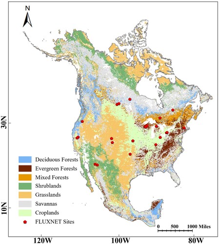
The study area covers the entire North American continent and includes a wide range of climatic characteristics, environmental conditions, terrain, and vegetation types. The study area (5° N to 9° N in latitude and 10° W to 175° W in longitude) has various biome types and contrasting climatic conditions based on factors such as solar radiation, temperature, and precipitation. These geographic characteristics make North America a preferable region for testing LAI vegetation models. Figure 1 shows a map of the vegetation types across North America and indicates the flux towers involved in this study.

Figure 1. The map of vegetation types across the continent of North America. The red points indicate the locations of flux tower sites.

2.2. Meteorological data

Daymet provides high-resolution (1 km) climatic variables that cover North America on a daily basis. It is derived from ground observations using both modeling and extrapolation approaches. The Daymet dataset was obtained from Oak Ridge National Laboratory (http://daymet.ornl.gov/). The variables for the period 2001–2016 include the daily minimum and maximum temperatures, daily precipitation, daily vapor pressure, day length, daily shortwave radiation, and daily snow water equivalent. These meteorological data have been used as forcing data for several terrestrial studies. In our study, these were resampled for an 8-day time period and used as model inputs for predicting vegetation growth.

2.3. Satellite data

An 8-day composite MODIS LAI product (MOD15A2H) from 2001 to 2016 with a spatial resolution of 1 km was used for the model training and testing. MOD15A2H provides an LAI that agrees well with site-based observations across seasons and biomes (Myneni et al. 2002). The LAI derived from MODIS has been widely used in land surface studies (Yuan et al. 2011). To mitigate cloud cover and aerosol contamination and improve data quality, the Savitzky–Golay method was adopted to obtain a smoothed eight-day time series. After smoothing, MOD15A2H LAI served as the target data in our machine learning modeling processes.

The Global Land Surface Satellite (GLASS) LAI product (version 6.0) has a temporal resolution of eight days and a spatial resolution of 500 m. It is derived from surface reflectance using a deep learning model. Liang et al. (2021) illustrated the superior accuracy of GLASS LAI product in time series, which exhibit enhanced spatiotemporal continuity, smoother temporal profiles, and fewer preprocessing requirements than the MODIS LAI. Therefore, the GLASS LAI (version 6.0) from 2009 to 2016 was used as a reference to be compared with the modeled LAI, though both GLASS LAI and MODIS LAI are derived from satellite-based surface reflectance data.

The MODIS land cover product (MCD12Q1) with a 500 m spatial resolution was utilized to distinguish different vegetation types. It covers the period from 2009 to 2016. The product was employed to categorize pixels into various vegetation types based on the International Geosphere–Biosphere Program classification. To facilitate a comparison with field data, the natural vegetation was classified into seven types: evergreen needleleaf forests (ENF), evergreen broadleaf forests (EBF), deciduous broadleaf forests (DBF), mixed forests (MF), shrublands (SHR; including open shrublands and closed shrublands), savannas (SAV; including woody savannas and savannas), and grassland (GRA). Because crop growth is influenced significantly by human activities and agricultural practices including planting, harvesting, and irrigation, croplands did not be utilized to predict the LAI time series in the developed model.

2.4. Site data

FLUXNET site data obtained from the Lawrence Berkeley National Laboratory in the U.S.A. were used for the site-scale validation of the developed model. FLUXNET is a global flux observation network based on widely distributed flux towers around the world. The FLUXNET site data are widely used for parameterizing and validating surface models. The updated FLUXNET 2015 released in 2016 provides over 200 variables, including meteorological and hydrological variables. In this study, FLUXNET 2015 sites with data records spanning over eight years were selected for site-scale validation. The selected variables included the minimum temperature, maximum temperature, precipitation, and shortwave radiation. The day length was obtained based on the location and date of the pixel. The vapor pressure deficit was calculated using the maximum and minimum temperature and humidity variables. A total of thirty-one sites satisfied these requirements. These included nine sites of DV (combined with DBF, DNF, and MF), 11 of EV (combined with ENF and EBF), and 11 of SDV (combined with SHR, SAV, and GRA). The geographical distribution of these sites is illustrated by the red sample plots in Figure 1.

2.5. Future climate data

The Climate Model Intercomparison Project 6 (CMIP6) states that improving and enhancing short-term climate projections remain a scientific priority (Eyring et al. 2016). In this study, three future Shared Socioeconomic Pathways (SSP) derived from CMIP6 (SSP126, SSP370, and SSP585) were introduced to predict vegetation LAI time series under future scenarios. SSP126 represents the lowest warming scenario with a radiative forcing of 2.6 W/m² in 2100, SSP370 represents a moderate warming scenario with a higher radiative forcing of 7.0 W/m² in 2100, and SSP585 represents the highest warming scenario with a radiative forcing of 8.5 W/m² in 2100. Daily climatic variables from the German Climate Computation Center (DKRZ) under three future scenarios was utilized to predict the LAI time series. These included the maximum and minimum temperature, humidity, shortwave radiation, precipitation, and land snow water equivalent. The LAI dataset from the DKRZ was selected for comparison with the modeled LAI. The selected climate datasets had a spatial resolution of 100 km. The period was 2015–2100.

3. Methods

3.1. AELSTM framework

The AELSTM developed in this study is an enhanced deep learning framework that learns the temporal relationships between meteorological variables and LAI time series. This is shown in Figure 2. The AELSTM has four layers: the input, LSTM, attention-enhanced, and output layers. In the input layer, a feature matrix denoted by {x₁, x₂, … , x_t} consisting of meteorological variables was constructed. The feature matrix is rearranged in temporal order after handling the outlier values, filtering, and normalization. The LSTM layer comprises a series of LSTM cells that selectively transmit and process memory information through a gating mechanism.

Figure 2. AELSTM model architecture. The attention enhanced layer is indicated by the red line. The red dashed boxes in the LSTM network den ote the memory flow of the forget gate, input gate, and output gate. In the feature matrix, T denotes the length of the time sequence, n denotes the input time steps, a-g represent the meteorological variables.

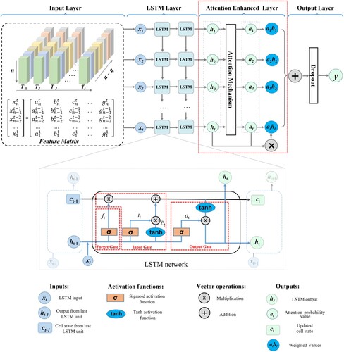
The forget gate is a pivotal element of the LSTM layer. It plays a key role in preserving the crucial features between the meteorological variables and LAI time series throughout multiple time-steps. The Sigmoid function in the LSTM cell determines which information in the final cell ${\mathrm{c}}_{t-1}$ needs to be forgotten. The forget gate is calculated as follows: (1) $f_t=\sigma ({\mathit{W}}_f\cdot [h_{t-1},x_t]+{\mathit{b}}_{\mathit{f}})$(1) The input gate determines the number of new features from $x_t$ that can be transferred to cell state ${\mathrm{c}}_t$. It involves two processes. First, the sigmoid function controls the information that should be updated to obtain $i_t$. Then, the tanh function creates the candidate vector ${\mathrm{c}}_t$. $f_t\cdot {\mathrm{c}}_{t-1}$ represents the information to be forgotten, and $i_t\cdot {\tilde{\mathrm{c}}}_t$ denotes the new memory to be added. Both these constitute the new cell state ${\mathrm{c}}_t$. The input gate is calculated as follows: (2) $i_t=\sigma ({\mathbf{W}}_i\cdot [{\mathrm{h}}_{t-1},{\mathrm{x}}_t]+{\mathbf{b}}_{\mathit{i}})$(2) (3) ${\tilde{c}}_t=\tanh ({\mathbf{W}}_c\cdot [{\mathrm{h}}_{t-1},{\mathrm{x}}_t]+{\mathbf{b}}_{\mathit{c}})$(3) (4) $c_t=f_t\cdot {\mathrm{c}}_{t-1}+i_t\cdot {\tilde{\mathrm{c}}}_t$(4)

The output gate controls the number of features in cell state ${\mathrm{c}}_t$ that should be output to ${\mathrm{h}}_t$. $o_t$ is the state of the output layer at time t. The Tanh function is run to the filter cell state ${\mathrm{c}}_t$. Then, the output ${\mathrm{h}}_t$ of the next time series is obtained. ${\mathit{W}}_{\mathit{f}}$、${\mathit{W}}_{\mathit{i}}$、${\mathit{W}}_{\mathit{c}}$、${\mathit{W}}_{\mathit{o}}$ are the weight matrices used to update the information in the hidden layer. ${\mathit{b}}_{\mathit{f}}$、${\mathit{b}}_{\mathit{i}}$、${\mathit{b}}_{\mathit{c}}$、${\mathit{b}}_{\mathit{o}}$ are the four bias vectors. The output gate is calculated as follows: (5) $o_t=\sigma ({\mathit{W}}_{\mathit{o}}\cdot [h_{t-1},x_t]+{\mathit{b}}_{\mathit{o}})$(5) (6) $h_t=o_t\cdot \tanh (c_t)$(6)

The LSTM demonstrated a higher accuracy than the other comparative models, as shown in Section 4.3. The original LSTM structure was optimized to predict vegetation LAI time series. An attention-enhanced layer was created between the LSTM and output layers to increase the network depth. This attention-enhanced layer generated attention values ${\mathit{a}}_{\mathit{t}}$ based on the LSTM output, which indicated the weight of each feature vector in predicting the vegetation LAI time series. The attention mechanism enables the AELSTM to focus on learning critical information by allocating more attention to key features and reducing the attention to secondary features. The attention-enhanced layer is calculated as follows: (7) $u_t=\tanh ({\mathit{W}}_{\mathit{w}}{h}_t+{\mathit{b}}_{\mathit{w}})$(7) (8) $a_t={\displaystyle \frac{\exp ({\mathit{u}}_{\mathit{t}}^{\mathit{T}}{\mathit{u}}_{\mathit{w}})}{{\sum }_{k=1}^T\exp ({\mathit{u}}_{\mathit{t}}^{\mathit{T}}{\mathit{u}}_{\mathit{w}})}}$(8) (9) $s=\sum a_t{\mathrm{h}}_t$(9) where ${\mathit{W}}_{\mathit{w}}$ and ${\mathit{u}}_{\mathit{w}}$ are the weight matrices of the attention mechanism indicating the information to be emphasized. ${\mathit{u}}_{\mathit{t}}$ is the result of the first weighting calculation; ${\mathit{b}}_{\mathit{w}}$ represents the deviation of the attention mechanism; and ${\mathit{h}}_t$ represents the input of the attention mechanism, which is the output of the LSTM hidden layer. ${\mathit{a}}_{\mathit{t}}$ is the final weight of ${\mathbf{h}}_{\mathit{t}}$, which is used to obtain the final output $\mathit{s}$. In the output layer, the dropout method is introduced to prevent the model from overfitting. After the inverse normalization process, the predicted LAI time series are output. The AELSTM conducts LAI prediction tasks on a per-pixel basis, rather than inputting a large number of samples to train a complex model. This pixel-based method trains an independent model at each pixel scale, which helps avoid mutual interference between mixed pixels and thus produces more accurate prediction results.

3.2. Comparative models

To identify a more suitable model for learning the temporal relationship between meteorological variables and LAI, three standard machine learning methods (support vector machine (SVM), random forest (RF), and convolutional neural network (CNN)) and four recurrent neural networks (recurrent neural networks (RNNs), long short-term memory (LSTM), gated recurrent unit (GRU), and bidirectional long short-term memory (BiLSTM)) were evaluated. These are commonly used for time-series prediction.

The SVM is a generalized linear classifier that uses supervised learning for binary classification. It is a standard kernel method (Hsieh 2009). The RF is an integrated learning method that improves prediction and classification by determining the optimal split points on each regression decision tree. A CNN extracts features through convolutional layers and uses pooling layers to reduce the dimensionality. This enables the extraction of multilevel features from a time series. The aforementioned machine learning methods can be applied to time-series modeling.

RNNs are suitable for processing time series because of their interlocking network structures (Bengio, Simard, and Frasconi 1994). As the prediction time increases, gradient explosion and disappearance during error backpropagation tend to limit the predictive capacity of RNNs. LSTM networks were proposed to improve the conventional RNN model (Sepp and Jürgen 1997). Its gating mechanism for controlling the information flow storage and updating can effectively overcome gradient explosion and disappearance problems. Moreover, it outperforms RNNs in processing long time-series tasks. The GRU has a simpler structure. Moreover, it displays faster computation than the LSTM because it contains only update and reset gates within the cell. BiLSTM is an optional RNN consisting of two unidirectional LSTM connections stacked in the reverse direction. With this architecture, the Bi-LSTM enables the capture of both forward and backward information in a time series at each time step.

3.3. Model implementation

Meteorological variables for the first eight years (2001–2008) were used to develop the AELSTM training program. The model predicted the LAI time series for the subsequent eight years (2009–2016). Ten percent of the time series within the training set was used to test the model for parameter tuning and optimization. After the experimental tests, the parameters for the AELSTM network were determined as follows: training batch of 50, learning rate of 0.01, input step size of 46, dropout rate of 20%, and two stacked LSTM layers. Finally, the AELSTM model was applied to predict the LAI time series for each pixel. This yielded a continuous AELSTM LAI dataset spanning 2009–2016. Note that AELSTM was constructed on a per-pixel basis to predict LAI time series, which means that the AELSTM on each pixel is independent. The AELSTM-predicted LAI was then compared with the MODIS LAI for validation across various biome types at the spatial and temporal scales.

To identify the performance of AELSTM for modeling LAI using meteorological variables, three widely used machine learning models and four recurrent neural networks were initially assessed. 5000 pixels were randomly selected from each biome type in North America to construct seven initial models. For fair comparisons, it was ensured that the input data were consistent across all models. In each comparison experiment only the models used for comparison were replaced. The performance of the AELSTM in predicting LAI time series was evaluated using FLUXNET sites across North America. Meteorological variables observed at FLUXNET sites were inputted into the AELSTM to predict LAI time series, which were then compared with LAI observations from MODIS under the same pixel.

To evaluate the potential of AELSTM coupled with a land surface model for predicting downstream variables, The predicted AELSTM LAI for the years 2009–2016 and the satellite-based MODIS LAI were separately inputted into the CoLM2014 model to predict the GPP. A description of the details of the CoLM and the process of calculating land-atmosphere fluxes can be found in (Dai et al. 2003; Ji and Dai 2010). The AELSTM model was evaluated for predicting the LAI time series for future scenarios. In this study, three future shared socioeconomic pathways (SSPs) of CMIP6 (SSP126, SSP370, and SSP585) were used to predict the vegetation LAI time series under future scenarios. We constructed the AELSTM model using meteorological data (consistent with meteorological variables in Daymet) from CMIP6 for 2020–2060 to predict a continuous LAI time series for the period 2060–2100.

3.4. Evaluation metrics

Three evaluation metrics that are commonly applied to machine learning studies were used to evaluate the model performance: Mean Absolute Error (MAE), Root Mean Square Error (RMSE), and Correlation Coefficient (R²). The calculation process of these three metrics is as follows: (10) $\mathrm{MAE}={\displaystyle \frac{1}{N}|y_t-{\hat{y}}_t|}$(10) (11) $\mathrm{RMSE}=\sqrt{{\displaystyle \frac{1}{N}\sum _{i=1}^N{(y_t-{\hat{y}}_t)}^2}}$(11) (12) ${\mathrm{R}}^2={\displaystyle \frac{{\sum }_{t=1}^N{({\hat{y}}_i-\overline{y})}^2}{{\sum }_{t=1}^N{(y_i-\overline{y})}^2}}$(12) where N denotes the sample count, $y_t$ signifies the observed value at time t, and ${\hat{y}}_t$ denotes the predicted value at time t.

4. Results

4.1. Spatiotemporal analysis

The spatial distributions of the AELSTM LAI, MODIS LAI, and MAE for the four days selected from the different seasons are shown in Figure 3. AELSTM effectively captured the spatial distribution characteristics of the LAI across all the seasons. In the majority of cases, the MAE between AELSTM LAI and MODIS LAI remained below 0.6 m²/m². The AELSTM did not exhibit significant deviations in these regions and displayed a high spatial consistency. During both spring and summer, vegetation grows vigorously under the influence of the humid subtropical climate of eastern North America, which has higher LAI values than other areas. Even for evergreen forests, where vegetation growth is continuous, the AELSTM model performed well in predicting the spatial distribution of the LAI. The western part of North America is dominated by cold semi-arid, hot desert, and warm-summer humid continental climates. This yields low LAI values. The LAI predicted by the AELSTM model is also consistent with the MODIS LAI. This result demonstrates that our machine learning model can effectively predict both seasonal and spatial distribution patterns of terrestrial vegetation LAI, thereby showing a higher similarity to the LAI obtained from satellite observations. The results demonstrate the effectiveness of our machine learning model in predicting both seasonal and spatial distribution patterns of terrestrial vegetation LAI. Thereby, it exhibited a higher similarity to satellite-driven LAI.

Figure 3. The spatial distributions AELSTM LAI, MODIS LAI, and MAE on four typical days in 2016: May 5 in spring, August 1 in summer, November 5 in autumn, and February 6 in winter. The fourth column shows the latitudinal profiles of the above LAI results where the shading denotes the standard deviation.

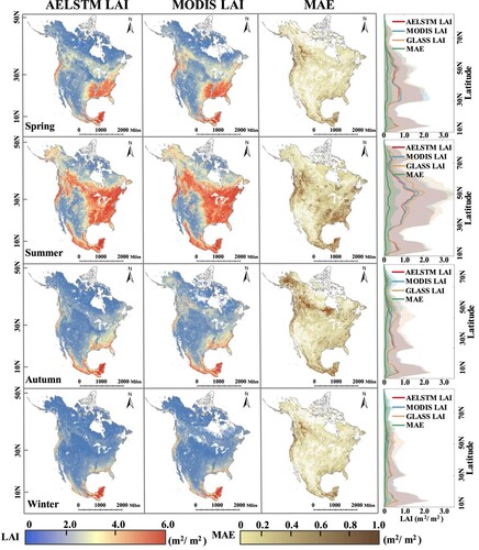
The right subfigure in Figure 3 shows the latitudinal averages of the modeled AELSTM LAI, MODIS LAI, and MAE. The corresponding GLASS LAI is used as reference. The distribution pattern of the AELSTM LAI along the latitudes is consistent with the satellite-derived MODIS LAI. At the latitudes 60–90 °N, the meteorological conditions are unfavorable for vegetation photosynthesis because of the low radiation flux and low temperatures. This results in slower plant growth and an indistinct seasonal cycle. In particular, in winter, when the polar night phenomenon occurs above 66.34 °N in the Northern Hemisphere, the vegetation growth is almost stagnant. As the latitude decreases, the meteorological conditions become favorable for vegetation growth, such as higher temperatures, enhanced rainfall, and longer daylight hours. This results in an increase in the LAI. AELSTM can also effectively capture these trends. The LAI produced is synchronized with the MODIS LAI.

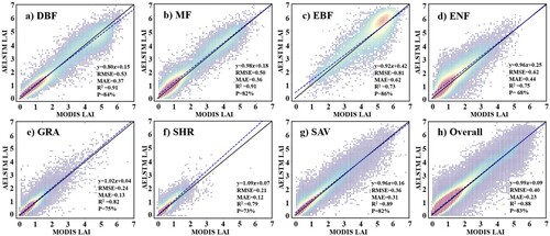
2000 pixels were randomly selected from Figure 4 to compare the AELSTM LAI and satellite-derived LAI time series. The results indicate that AELSTM could accurately predict the LAI. Moreover, it demonstrated a high correlation with the MODIS LAI, exhibiting an overall R² of 0.88, RMSE of 0.40 m²/m², and MAE of 0.23 m²/m² under the seven biome types. Describing the uncertainties associated with LAI products is vital for downstream applications (Gobron and Verstraete 2009; Lafont et al. 2012). The LAI application communities require a maximum uncertainty of 20% (Fang et al. 2019). The uncertainty in the AELSTM LAI varied by biome type, as shown in Figure 4. Overall, 83% of the pixels in the predicted AELSTM LAI time series satisfied the deterministic requirements for global climate modeling studies.

Figure 4. Comparison of AELSTM LAI and MODIS LAI under different biome types. P is the percentage of image elements with uncertainty within 20%. The blue dashed line is the fit line.

Figure 5 compares the time series of the AELSTM LAI, MODIS LAI, GLASS LAI, and FLUXNET LAI across various ground sites from 2009 to 2016 (excluding EBF owing to the absence of suitable FLUXNET sites). The results show that the AELSTM LAI has an LAI time series consistent with the satellite-derived LAI. The R² values between AELSTM LAI and MODIS LAI range from 0.88 to 0.97 and those between AELSTM LAI and GLASS LAI range from 0.84 to 0.96. The AELSTM model effectively learned the seasonal variation characteristics of LAI during vegetation growth. The forest vegetation types (Figure 5a–d) exhibited a more significant seasonal variation and larger LAI than the non-forest vegetation types (Figure 5e–g).

Figure 5. Comparison of AELSTM LAI, MODIS LAI, GLASS LAI, and FLUXNET LAI at ground sites across various biome types from 2009 to 2016. The name and coordinates of each FLUXNET site are indicated in the upper left corner of the subplot. The R² values marked with black, blue, and orange indicate the correlation coefficient between the AELSTM LAI and the MODIS LAI GLASS LAI, FLUXNET LAI, respectively.

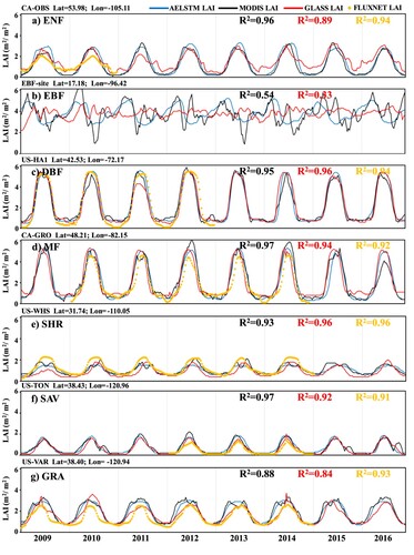
A site-level validation of the AELSTM was conducted to predict the LAI time series on FLUXNET sites. The FLUXNET LAI represents the results predicted using meteorological variables collected from the FLUXNET 2015 sites. Meteorological variables from FLUXNET 2015 and Daymet were input individually into the AELSTM model, and consistent LAI time series were obtained at the corresponding site. In Figure 5, the R² between the FLUXNET LAI and AELSTM LAI is larger than 0.91 across different FLUXNET sites. These time-series subplots demonstrate the capability of AELSTM to predict continuous LAI time series, capture vegetation growth seasonality, and correspond to the results predicted at the site scale.

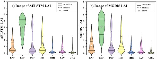
To compare the differences between the AELSTM LAI and MODIS LAI, 5000 sample pixels of the LAI time series were randomly selected from each biome type across North America. Figure 6 illustrates the approximate ranges of both modeled and satellite-derived LAI for different biome types. The 20–75% separator, median, and mean values of the AELSTM and MODIS LAI were similar in the time series for each biome type. The forest biomes (ENF, EBF, DBF, and MF) had larger LAI values and a wider range than the non-forest biomes (SHR, SAV, and GRA). For the evergreen forest types (ENF and EBF), which exhibit continuous growth and no significant variations over time, the LAI values predicted by the AELSTM model tended to be average. Therefore, the approximate range of the AELSTM LAI was more concentrated in the evergreen forest types. For the non-evergreen forest types (DBF, MF, SHR, SAV, and GRA), the approximate ranges of the AELSTM LAI and MODIS LAI were almost identical.

Figure 6. The approximate ranges of AELSTM LAI and MODIS LAI for different biome types.

Figure 7 shows the biome-specific seasonal variation in the AELSTM performance metrics (MAE and R²) over the days of the year. The forest biomes have a higher MAE (with a maximum of 0.5 m²/ m²) than the non-forest biomes (a maximum MAE of 0.3 m²/ m²). The MAE values of the AELSTM model are high (0.3–0.5 m²/ m²) in summer. However, the values are low (up to 0.1–0.3 m²/ m²) in winter. The R² values are generally higher than 0.9 in summer and could attain 0.6 in winter.

Figure 7. The 8-year averaged MAE and R² (indicated by different colors) between AELSTM LAI and MODIS LAI from 2009 to 2016 for different biome types over the day of year.

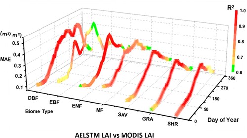
In most cases wherein the model had higher MAE values, the R² values tended to be higher. This was because vegetation grows actively in summer and because the LAI values were higher, which caused higher deviations in the modeled MAE values. In contrast, the vegetation LAI values were lower in winter, which resulted in lower modeled MAE values. During the vegetative growth season, the LAI time series varied more significantly with meteorological variables and showed more regular variations. Moreover, the AELSTM model learned the characteristic variations between meteorological variables and LAI. It showed a higher R². During winter, when the vegetation became inactive, the LAI time series did not show significant variations in meteorological variables. This resulted in a lower R². The prediction capability of AELSTM for different biome types displayed seasonal fluctuations. However, the overall performance was remarkable. It enabled the effective prediction of the time series of vegetation LAI.

4.2. Model assessment

Table 1 compares the performance of AELSTM with that of other machine learning and deep learning models in predicting the LAI time series. The natural vegetation types were classified into three categories: deciduous vegetation (DV), characterized by one growing season per year and encompassing deciduous needleleaf forests, deciduous broadleaf forests, and mixed forests; evergreen vegetation (EV), which has a persistent year-round growing season and includes evergreen needle leaf and broadleaf forests; and stressed deciduous vegetation (SDV), which exhibits the potential for multiple growing seasons within a year and includes closed shrublands, open shrublands, woody savannas, savannas, and grasslands. Among the seven machine models, the LSTM exhibited the highest prediction accuracy (R² ranged from 0.85 to 0.90) under different biome types. It captured the characteristic associations between the meteorological variables and the LAI time series more effectively. Therefore, the LSTM was selected to incorporate an attention mechanism layer to enhance the model. According to Table 1, the evaluation results reveal that the AELSTM model achieved an optimal prediction performance (R² = 0.90-0.93).

Table 1. Model evaluation of the machine learning and deep learning models.

Models		DV			EV			SDV
	R^2	RMSE m^2/m^2	MAE m^2/m^2	R^2	RMSE m^2/m^2	MAE m^2/m^2	R^2	RMSE m^2/m^2	MAE m^2/m^2
AELSTM	0.93	0.473	0.314	0.90	0.498	0.288	0.92	0.202	0.115
GRU	0.85	0.613	0.41	0.79	0.732	0.533	0.86	0.285	0.163
BiLSTM	0.86	0.682	0.421	0.83	0.597	0.426	0.83	0.353	0.189
RNN	0.79	0.860	0.482	0.82	0.634	0.418	0.84	0.336	0.176
LSTM	0.90	0.545	0.391	0.85	0.593	0.386	0.88	0.268	0.147
RF	0.87	0.578	0.436	0.83	0.638	0.436	0.86	0.335	0.207
CNN	0.81	0.71	0.523	0.81	0.662	0.424	0.83	0.351	0.236
SVM	0.84	0.637	0.457	0.76	0.684	0.581	0.85	0.318	0.186

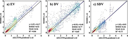
To validate the AELSTM performance at the site scale, ground-based meteorological variables from 31 FLUXNET sites in North America were used for the validation experiments. Figure 8 compares the AELSTM LAI based on the FLUXNET meteorological variables with the MODIS LAI at the corresponding pixel. The results demonstrate that the R² values of DV and EV exceeded 0.85 and that of SDV was 0.73. The AELSTM model can effectively predict the LAI time series for different biome types at the site scale.

Figure 8. AELSTM model validation at FLUXNET sites. The scatter density plots illustrate the comparisons between the satellite-derived LAI and AELSTM-predicted LAI for various vegetation types at the site scale.

4.3. Predicting GPP by coupling with CoLM

As illustrated in Figure 9, the spatial distributions of GPP in 2016 obtained by the CoLM2014 model using the AELSTM LAI and satellite-driven LAI were consistent and displayed similar latitudinal variations. Figure 9(a and b) reveals that GPP exhibits low values in northern North America and high values in southern North America in summer (July 1), when vegetation displays peak activity. Figure 9(c and d) shows that the vegetation activity in the northern area of North America is nearly stagnant in winter (February 1st), whereas the capability of southern vegetation to sequester carbon is limited. The spatial distribution pattern of the GPP in Figure 9 is consistent with that of the LAI in Figure 3.

Figure 9. Comparison of the GPP results from the CoLM2014 using MODIS LAI and AELSTM LAI. Subplot (a) and (c) show the GPP predicted using the AELSTM LAI. Subplot (b) and (d) show the GPP predicted using the MODIS LAI. Subplot (e) and (f) present the latitudinal GPP averages, where the shading denotes the standard deviation. The scatter plots in subplot (a) and (c) show the regression analysis of predicted GPP using MODIS LAI and AELSTM LAI from CoLM.

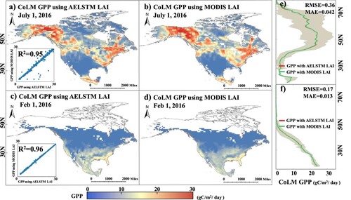
As shown in Figure 9(a and c), predicted GPP using MODIS LAI and AELSTM LAI in CoLM demonstrate a high correlation, with R² values of 0.95 in summer (July 1) and 0.96 in winter (February 1st). Figure 9(e and f) depict the latitude profiles of predicted GPP results, showing small differences in the latitudinal average lines between these two categories of GPP. In summer and winter, the RMSE values were 0.36 and 0.17 m²/m², whereas the MAE values were 0.042 and 0.013 m²/m², respectively. These results demonstrate that the AELSTM and MODIS LAI have a high degree of consistency in predicting GPP when used as the input LAI for the CoLM2014 model. Coupling AELSTM with the land surface model can effectively predict land–atmosphere fluxes such as the GPP.

4.4. Predicting LAI under future climate scenarios

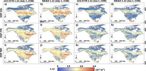
Figure 10 illustrates the predicted AELSTM LAI in North America for 2060–2100 under three climate scenarios (SSP126, SSP370, and SSP585) using climate variables from CMIP6. The AELSTM LAI on January 1 and July 1, 2100, were selected as examples for comparison with the predicted LAI (obtained from the DKRZ) in CMIP6. AELSTM effectively predicts high values of LAI in the central and southeastern regions of North America, and low values of LAI in the northern and southwestern regions. The spatial distribution of the AELSTM LAI is highly consistent with that of the DKRZ LAI in both winter and summer. Different climate scenarios have unique atmospheric processes that result in differences in the spatial distribution of the predicted LAI. Under an identical scenario, the spatial distributions of the AELSTM and DKRZ LAI were similar.

Figure 10. The spatial distribution of AELSTM LAI predicted under three shared socioeconomic pathways (SSPs), compared with that for CMIP6 LAI. Panel (a)–(d), (e)–(h), and (i)–(l) show the predicted LAI results under SSP 126, SSP 370, and SSP 585, respectively.

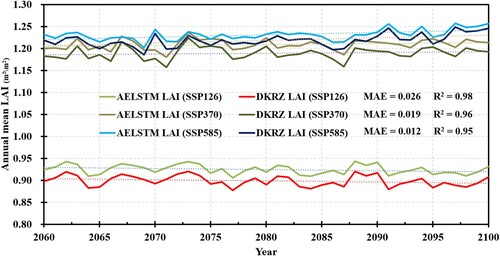
Figure 11 illustrates the temporal trends in the annual average AELSTM and DKRZ LAI from 2060 to 2100. The predicted annual average AELSTM LAI aligned well with the annual average DKRZ LAI. The R² values between the annual mean AELSTM LAI and the annual mean DKRZ LAI were higher than 0.95, and the MAE values were below 0.026 m²/m² across the different scenarios. The LAI of SSP370 and SSP585 were higher than that of SSP126. The predicted AELSTM LAI was consistent with the DKRZ LAI in the time series. No anomalous year was observed. These results indicate that AELSTM captures the implicit relationship between climatic variables and vegetation processes under different scenarios. This would enable the effective prediction of vegetation LAI time series.

Figure 11. Time series of annual mean AELSTM LAI predicted under three SSPs from 2060 to 2100, compared with that for DKRZ LAI. The R² and MAE indicate the AELSTM performance under SSP126, SSP370, and SSP585, respectively.

5. Discussion

A pixel-based method was adopted to model the LAI time series in this research. Another common modeling approach used in many studies is the biome-based method. It selects a large number of samples according to the biome type to model the vegetation activity (Ma and Liang 2022; Zhang, Xin, and Li 2021; Zhou et al. 2023). Biome-based methods assume that each type of biome responds similarly to environmental variations. Therefore, these methods select a large number of samples directly from each vegetation type to train the model. Because of the effects of pixel mixture, each pixel at a moderate or coarse spatial resolution typically contains several vegetation types. Thus, representative and pure endmembers for both model training and testing are crucial but selecting these pixels is challenging (Yuan et al. 2020). Vegetative activity may differ across pixels under identical climatic conditions even when these pixels are classified under the same biome type. Compared with the biome-based method, the pixel-based method models each pixel individually and generates more accurate outcomes when predicting LAI across large geographic regions.

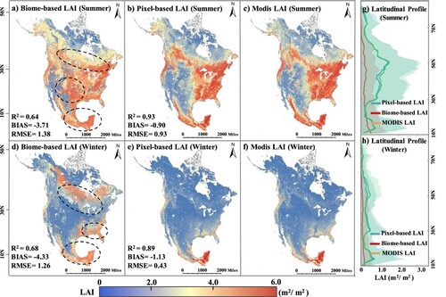
Thus, the pixel-based method enables the model to learn the spatiotemporal characteristics of vegetative growth without interference from other pixels. Figure 12 compared the results of the model LAI obtained using the biome-based and pixel-based methods. The AELSTM LAI modeled using the biome-type method exhibited differences from the MODIS LAI in most regions of North America (indicated using dashed lines in Figure 12). The pixel-based method improved the results and reduced the RMSE and BIAS values. The R² values increased from 0.64 to 0.93 in summer and 0.68 to 0.89 in winter, respectively. This pixel-based method prevents mutual interference between pixels and improves the predictive performance of the AELSTM model.

Figure 12. Comparison of the predicted LAI results using different modeling methods in summer and winter. The first column shows the AELSTM LAI obtained using the pixel-based method, the second column shows that obtained using the biome-based method, the third column shows the MODIS LAI for reference, and the fourth column shows the latitudinal profiles of the above LAI results where the shading denotes the standard deviation. The metrics (R², BIAS, RMSE) in subplot (a), (b) and (d), (e) are calculated with MODIS LAI.

The predictive model should have a higher sensitivity to more critical meteorological variables that affect vegetation activity. A specific variable was removed from the modeling process to assess the sensitivity of AELSTM to this variable. The variations in the model performance are presented in Table 2. When using AELSTM to predict LAI time series, day length, maximum and minimum temperature have greater changes on model performance. In particular, the RMSE increased by 0.84 m²/m² after the day length variable was removed (as shown in Table 2). This is consistent with our observation that both day length and air temperature are closely associated with vegetation activity. Among the seven meteorological variables, precipitation exhibited the lowest sensitivity to the AELSTM. Although precipitation is one of the key drivers of an ecosystem and has a considerable effect on vegetation activity (Abel et al. 2021), the AELSTM model does not effectively utilize precipitation. This indicates that the machine learning model also has difficulty in learning the implicit association between precipitation and vegetation activity. Although the contribution of precipitation to the machine learning model is limited, the predicted LAI time series still demonstrated a reasonable accuracy and can be utilized effectively in downstream applications.

Table 2. Variations in model performance after a specific meteorological variable is omitted.

	Day length	Maximum temperatures	Minimum temperatures	Vapor pressure	Shortwave radiation	Snow water equivalent	Precipitation
RMSE	0.84	0.14	0.13	0.10	0.09	0.08	0.04
MAE	0.63	0.12	0.11	0.08	0.08	0.06	0.02
R^2	-0.10	-0.04	-0.03	-0.02	-0.02	-0.02	-0.01

As a data-driven approach, machine learning models are challenging in terms of interpreting the underlying physiological and ecological mechanisms (Reichstein et al. 2019). Therefore, machine learning should not be considered a substitute for process-based models. Physics-guided machine learning models provide benchmarking accuracy when developing physical models based on physiological or ecological mechanisms. Moreover, machine-learning models can serve as intermediary solutions in cases where our scientific understanding of specific processes such as predicting vegetation activity remains limited. This would facilitate the development of novel mechanistic models. In future research, it is worthy testing to incorporate the physical processes of vegetation growth into deep learning models to generate predictions that better adhere to physical constraints on a global scale.

6. Conclusions

Predicting vegetation LAI time series is crucial for understanding land surface vegetation dynamics and their response to climate and environmental variations. Unlike diagnostic numerical models, a meteorological data-driven AELSTM model was proposed to predict vegetation LAI time series. Our results reveal that AELSTM outperformed the other tested machine learning and deep learning models including RNN, LSTM, GRU, BiLSTM, SVM, RF, and CNN in predicting the LAI time series. The AELSTM-predicted LAI maintained a high consistency with satellite-based LAI. Here, the R² between the modeled and observed LAI was 0.86, 0.93, and 0.92 for EV, DV, and SDV, respectively. Coupling the AELSTM model with CoLM2014 can effectively predict land–atmosphere fluxes such as vegetation GPP. AELSTM can accurately predict vegetation LAI time series under three climate scenarios (SSP126, SSP370, and SSP585) using CMIP6. This study has provided a more accurate approach for predicting LAI time series. It can serve as a benchmark for improving land surface models for predicting vegetation ecological dynamics.

Data availability statement

The authors thank Dai et al for providing the common land model (CoLM) Version 2014 code through the site: http://globalchange.bnu.edu.cn/research. The MODIS data sets including MOD15A2H, MCD12Q1, and MOD17 are available from https://ladsweb.modaps.eosdis.nasa.gov/search/order. The GLASS LAI product (version 6.0) is available for download from http://www.glass.umd.edu/Download.html. The FLUXNET 2015 is available at https://fluxnet.org/data/fluxnet2015-dataset. The Daymet dataset was downloaded from the Oak Ridge National Laboratory at http://daymet.ornl.gov/. We downloaded daily future climatic variables from the German Climate Computation Center (DKRZ) in Climate Model Intercomparison Project 6 (CMIP6) at https://esgf-node.ipsl.upmc.fr/search/cmip6-ipsl/. The AELSTM model package we proposed and code for analyses are available on the authors’ personal zenodo at https://zenodo.org/records/10395982. We welcome researchers and academics to further evaluate and improve the proposed model.

Acknowledgments

The authors thank anonymous reviewers for their constructive comments.

Disclosure statement

No potential conflict of interest was reported by the author(s).

Additional information

Funding

This research is supported by National Natural Science Foundation of China [grant number 42371483] and Guangdong Basic and Applied Basic Research Foundation [grant number 2022B1515130001].

References

- Abel, C., S. Horion, T. Tagesson, W. De Keersmaecker, A. W. R. Seddon, A. M. Abdi, and R. Fensholt. 2021. “The Human-Environment Nexus and Vegetation-Rainfall Sensitivity in Tropical Drylands.” Nature Sustainability 4 (1): 25–32. https://doi.org/10.1038/s41893-020-00597-z.
- Baker, I. T., L. Prihodko, A. S. Denning, M. Goulden, S. Miller, and H. R. Da Rocha. 2008. “Seasonal Drought Stress in the Amazon: Reconciling Models and Observations.” Journal of Geophysical Research: Biogeosciences 113. https://doi.org/10.1029/2007JG000644.
- Bengio, Y., P. Simard, and P. Frasconi. 1994. “Learning Long-Term Dependencies with Gradient Descent is Difficult.” IEEE Transactions on Neural Networks 5 (2): 157–166. https://doi.org/10.1109/72.279181.
- Chen, M., E. K. Melaas, J. M. Gray, M. A. Friedl, and A. D. Richardson. 2016. “A new Seasonal-Deciduous Spring Phenology Submodel in the Community Land Model 4.5: Impacts on Carbon and Water Cycling Under Future Climate Scenarios.” Global Change Biology 22 (11): 3675–3688. https://doi.org/10.1111/gcb.13326.
- Chen, J. M., G. Mo, J. Pisek, J. Liu, F. Deng, M. Ishizawa, and D. Chan. 2012. “Effects of Foliage Clumping on the Estimation of Global Terrestrial Gross Primary Productivity.” Global Biogeochemical Cycles 26 (1). https://doi.org/10.1029/2010GB003996.
- Chen, M., G. R. Willgoose, and P. M. Saco. 2015. “Investigating the Impact of Leaf Area Index Temporal Variability on Soil Moisture Predictions Using Remote Sensing Vegetation Data.” Journal of Hydrology 522: 274–284. https://doi.org/10.1016/j.jhydrol.2014.12.027.
- Dai, W., H. Jin, Y. Zhang, T. Liu, and Z. Zhou. 2019. “Detecting Temporal Changes in the Temperature Sensitivity of Spring Phenology with Global Warming: Application of Machine Learning in Phenological Model.” Agricultural and Forest Meteorology 279: 107702. https://doi.org/10.1016/j.agrformet.2019.107702.
- Dai, Y., X. Zeng, R. E. Dickinson, I. Baker, G. B. Bonan, M. G. Bosilovich, A. S. Denning, et al. 2003. “The Common Land Model.” Bulletin of the American Meteorological Society 84 (84): 1013–1024. https://doi.org/10.1175/BAMS-84-8-1013.
- Ding, Y., Y. Zhu, J. Feng, P. Zhang, and Z. Cheng. 2020. “Interpretable Spatio-Temporal Attention LSTM Model for Flood Forecasting.” Neurocomputing 403: 348–359. https://doi.org/10.1016/j.neucom.2020.04.110.
- Eyring, V., S. Bony, G. A. Meehl, C. A. Senior, B. Stevens, R. J. Stouffer, and K. E. Taylor. 2016. “Overview of the Coupled Model Intercomparison Project Phase 6 (CMIP6) Experimental Design and Organization.” Geoscientific Model Development 9 (5): 1937–1958. https://doi.org/10.5194/gmd-9-1937-2016.
- Fang, H., F. Baret, S. Plummer, and G. Schaepman Strub. 2019. “An Overview of Global Leaf Area Index (LAI): Methods, Products, Validation, and Applications.” Reviews of Geophysics 57 (3): 739–799. https://doi.org/10.1029/2018RG000608.
- Foley, J. A., I. C. Prentice, N. Ramankutty, S. Levis, D. Pollard, S. Sitch, and A. Haxeltine. 1996. “An Integrated Biosphere Model of Land Surface Processes, Terrestrial Carbon Balance, and Vegetation Dynamics.” Global Biogeochemical Cycles 10 (4): 603–628. https://doi.org/10.1029/96GB02692.
- Ge, H., Z. Yan, W. Yu, and L. Sun. 2019. “An Attention Mechanism Based Convolutional LSTM Network for Video Action Recognition.” Multimedia Tools and Applications 78 (14): 20533–20556. https://doi.org/10.1007/s11042-019-7404-z.
- Gobron, N., and M. M. Verstraete. 2009. “Assessment of the Status of the Development of the Standards for the Terrestrial Essential Climate Variables: Leaf Area Index (LAI).” http://www.fao.org/gtos/doc/ECVs/T11/T11.pdf.
- Grant, R. F., A. G. Barr, T. A. Black, H. A. Margolis, A. L. Dunn, J. Metsaranta, S. Wang, J. H. McCaughey, and C. A. Bourque. 2009. “Interannual Variation in net Ecosystem Productivity of Canadian Forests as Affected by Regional Weather Patterns - A Fluxnet-Canada Synthesis.” Agricultural and Forest Meteorology 149 (11): 2022–2039. https://doi.org/10.1016/j.agrformet.2009.07.010.
- Greff, K., R. K. Srivastava, J. Koutník, B. R. Steunebrink, and J. Schmidhuber. 2016. “LSTM: A Search Space Odyssey.” IEEE Transactions on Neural Networks and Learning Systems 28 (10): 2222–2232. https://doi.org/10.1109/TNNLS.2016.2582924.
- Gui, Z., Y. Sun, L. Yang, D. Peng, F. Li, H. Wu, C. Guo, W. Guo, and J. Gong. 2021. “LSI-LSTM: An Attention-Aware LSTM for Real-Time Driving Destination Prediction by Considering Location Semantics and Location Importance of Trajectory Points.” Neurocomputing 440: 72–88. https://doi.org/10.1016/j.neucom.2021.01.067.
- Gunlu, A., and S. Bulut. 2023. “Modeling Leaf Area Index Using Time-Series Remote Sensing and Topographic Data in Pure Anatolian Black Pine Stands.” International Journal of Environmental Science and Technology 20 (5): 5471–5490. https://doi.org/10.1007/s13762-022-04552-7.
- Ham, Y., J. Kim, and J. Luo. 2019. “Deep Learning for Multi-Year ENSO Forecasts.” Nature 573 (7775): 568–572. https://doi.org/10.1038/s41586-019-1559-7.
- Houborg, R., and M. F. McCabe. 2018. “A Hybrid Training Approach for Leaf Area Index Estimation via Cubist and Random Forests Machine-Learning.” ISPRS Journal of Photogrammetry and Remote Sensing 135: 173–188. https://doi.org/10.1016/j.isprsjprs.2017.10.004.
- Hsieh, W. W. 2009. Machine Learning Methods in the Environmental Sciences: Neural Networks and Kernels. Vancouver: Cambridge university press.
- Hu, Z., H. Shi, K. Cheng, Y. Wang, S. Piao, Y. Li, L. Zhang, et al. 2018. “Joint Structural and Physiological Control on the Interannual Variation in Productivity in a Temperate Grassland: A Data-Model Comparison” Global Change Biology 24 (7): 2965–2979. https://doi.org/10.1111/gcb.14274.
- Ji, D., and Y. Dai. 2010. The Common Land Model (CoLM) Technical Guide. Beijing, People’s Republic of China: Beijing Normal University.
- Kolby Smith, W., S. C. Reed, C. C. Cleveland, A. P. Ballantyne, W. R. L. Anderegg, W. R. Wieder, Y. Y. Liu, and S. W. Running. 2016. “Large Divergence of Satellite and Earth System Model Estimates of Global Terrestrial CO2 Fertilization” Nature Climate Change 6 (3): 306–310. https://doi.org/10.1038/nclimate2879.
- Krinner, G., N. Viovy, N. de Noblet-Ducoudré, J. Ogée, J. Polcher, P. Friedlingstein, P. Ciais, S. Sitch, and I. C. Prentice. 2005. “A Dynamic Global Vegetation Model for Studies of the Coupled Atmosphere-Biosphere System” Global Biogeochemical Cycles 19 (1): GB1015. https://doi.org/10.1029/2003GB002199.
- Lafont, S., Y. Zhao, J. C. Calvet, P. Peylin, P. Ciais, F. Maignan, and M. Weiss. 2012. “Modelling LAI, Surface Water and Carbon Fluxes at High-Resolution Over France: Comparison of ISBA-A-gs and ORCHIDEE” Biogeosciences (Online) 9 (1): 439–456. https://doi.org/10.5194/bg-9-439-2012.
- Lawrence, D. M., R. A. Fisher, C. D. Koven, K. W. Oleson, S. C. Swenson, G. Bonan, N. Collier, et al. 2019. “The Community Land Model Version 5: Description of new Features, Benchmarking, and Impact of Forcing Uncertainty.” Journal of Advances in Modeling Earth Systems 11 (12): 4245–4287. https://doi.org/10.1029/2018MS001583.
- Li, Q., Y. Zhu, W. Shangguan, X. Wang, L. Li, and F. Yu. 2022. “An Attention-Aware LSTM Model for Soil Moisture and Soil Temperature Prediction.” Geoderma 409: 115651. https://doi.org/10.1016/j.geoderma.2021.115651.
- Liang, S., J. Cheng, K. Jia, B. Jiang, Q. Liu, Z. Xiao, Y. Yao, et al. 2021. “The Global Land Surface Satellite (GLASS) Product Suite.” Bulletin of the American Meteorological Society 102 (2): E323–E337. https://doi.org/10.1175/BAMS-D-18-0341.1.
- Ma, H., and S. Liang. 2022. “Development of the GLASS 250-m Leaf Area Index Product (Version 6) from MODIS Data Using the Bidirectional LSTM Deep Learning Model.” Remote Sensing of Environment 273: 112985. https://doi.org/10.1016/j.rse.2022.112985.
- Myneni, R. B., S. Hoffman, Y. Knyazikhin, J. L. Privette, J. Glassy, Y. Tian, Y. Wang, et al. 2002. “Global Products of Vegetation Leaf Area and Fraction Absorbed PAR from Year one of MODIS Data.” Remote Sensing of Environment 83 (1): 214–231. https://doi.org/10.1016/S0034-4257(02)00074-3.
- Piao, S., Q. Liu, A. Chen, I. A. Janssens, Y. Fu, J. Dai, L. Liu, X. Lian, M. Shen, and X. Zhu. 2019. “Plant Phenology and Global Climate Change: Current Progresses and Challenges.” Global Change Biology 25 (6): 1922–1940. https://doi.org/10.1111/gcb.14619.
- Reichstein, M., G. Camps-Valls, B. Stevens, M. Jung, J. Denzler, N. Carvalhais, and Prabhat. 2019. “Deep Learning and Process Understanding for Data-Driven Earth System Science.” Nature 566 (7743): 195–204. https://doi.org/10.1038/s41586-019-0912-1.
- Restrepo-Coupe, N., N. M. Levine, B. O. Christoffersen, L. P. Albert, J. Wu, M. H. Costa, D. Galbraith, et al. 2017. “Do Dynamic Global Vegetation Models Capture the Seasonality of Carbon Fluxes in the Amazon Basin? A Data-Model Intercomparison” Global Change Biology 23 (1): 191–208. https://doi.org/10.1111/gcb.13442.
- Richardson, A. D., R. S. Anderson, M. A. Arain, A. G. Barr, G. Bohrer, G. Chen, J. M. Chen, et al. 2012. “Terrestrial Biosphere Models Need Better Representation of Vegetation Phenology: Results from the North American Carbon Program Site Synthesis.” Global Change Biology 18 (2): 566–584. https://doi.org/10.1111/j.1365-2486.2011.02562.x.
- Schaphoff, S., W. von Bloh, A. Rammig, K. Thonicke, H. Biemans, M. Forkel, D. Gerten, et al. 2018. “LPJmL4 – a Dynamic Global Vegetation Model with Managed Land – Part 1: Model Description” Geoscientific Model Development 11 (4): 1343–1375. https://doi.org/10.5194/gmd-11-1343-2018.
- Sepp, H., and S. Jürgen. 1997. “Long Short-Term Memory.” Neural Computation 9 (8): 1735–1780. https://doi.org/10.1162/neco.1997.9.8.1735.
- Sezer, O. B., M. U. Gudelek, and A. M. Ozbayoglu. 2020. “Financial Time Series Forecasting with Deep Learning: A Systematic Literature Review: 2005–2019” Applied Soft Computing 90: 106181. https://doi.org/10.1016/j.asoc.2020.106181.
- Stöckli, R., T. Rutishauser, D. Dragoni, J. O'Keefe, P. E. Thornton, M. Jolly, L. Lu, and A. S. Denning. 2008. “Remote Sensing Data Assimilation for a Prognostic Phenology Model.” Journal of Geophysical Research: Biogeosciences 113 (G4). https://doi.org/10.1029/2008JG000781.
- Thornton, P. E., B. E. Law, H. L. Gholz, K. L. Clark, E. Falge, D. S. Ellsworth, A. H. Goldstein, et al. 2002. “Modeling and Measuring the Effects of Disturbance History and Climate on Carbon and Water Budgets in Evergreen Needleleaf Forests.” Agricultural and Forest Meteorology 113 (1): 185–222. https://doi.org/10.1016/S0168-1923(02)00108-9.
- Tian, H., P. Wang, K. Tansey, D. Han, J. Zhang, S. Zhang, and H. Li. 2021. “A Deep Learning Framework Under Attention Mechanism for Wheat Yield Estimation Using Remotely Sensed Indices in the Guanzhong Plain, PR China.” International Journal of Applied Earth Observation and Geoinformation 102: 102375. https://doi.org/10.1016/j.jag.2021.102375.
- Verger, A., I. Filella, F. Baret, and J. Peñuelas. 2016. “Vegetation Baseline Phenology from Kilometric Global LAI Satellite Products.” Remote Sensing of Environment 178: 1–14. https://doi.org/10.1016/j.rse.2016.02.057.
- Xin, Q., Y. Dai, X. Li, X. Liu, P. Gong, and A. D. Richardson. 2018. “A Steady-State Approximation Approach to Simulate Seasonal Leaf Dynamics of Deciduous Broadleaf Forests via Climate Variables.” Agricultural and Forest Meteorology 249: 44–56. https://doi.org/10.1016/j.agrformet.2017.11.025.
- Xin, Q., X. Zhou, N. Wei, H. Yuan, Z. Ao, and Y. Dai. 2020. “A Semiprognostic Phenology Model for Simulating Multidecadal Dynamics of Global Vegetation Leaf Area Index.” Journal of Advances in Modeling Earth Systems 12 (7). https://doi.org/10.1029/2019MS001935.
- Yuan, H., Y. Dai, Z. Xiao, D. Ji, and W. Shangguan. 2011. “Reprocessing the MODIS Leaf Area Index Products for Land Surface and Climate Modelling.” Remote Sensing of Environment 115 (5): 1171–1187. https://doi.org/10.1016/j.rse.2011.01.001.
- Yuan, Q., H. Shen, T. Li, Z. Li, S. Li, Y. Jiang, H. Xu, et al. 2020. “Deep Learning in Environmental Remote Sensing: Achievements and Challenges.” Remote Sensing of Environment 241: 111716. https://doi.org/10.1016/j.rse.2020.111716.
- Zhang, Z., Q. Xin, and W. Li. 2021. “Machine Learning-Based Modeling of Vegetation Leaf Area Index and Gross Primary Productivity Across North America and Comparison with a Process-Based Model.” Journal of Advances in Modeling Earth Systems 13(10). https://doi.org/10.1029/2021MS002802.
- Zhou, X., Q. Xin, S. Zhang, S. Delzon, and Y. Dai. 2023. “A Prognostic Vegetation Phenology Model to Predict Seasonal Maximum and Time Series of Global Leaf Area Index Using Climate Variables.” Agricultural and Forest Meteorology 342: 109739. https://doi.org/10.1016/j.agrformet.2023.109739.