A combined multi-source data and deep learning approach for retrieving snow depth on Antarctic Sea ice during the melting season

ABSTRACT

Snow on the Antarctic sea ice is a crucial component of the cryosphere. In response to the dynamic and highly heterogeneous Antarctic snow during the sea ice melting season, this study employed a combined multi-source data and deep learning method to accurately retrieve snow depth on Antarctic sea ice. Initially, we integrate multiple datasets, including satellite remote sensing, geospatial information, and meteorological data. Subsequently, a Convolutional Neural Network (CNN) is utilized to construct a snow depth retrieval model (PSDCNN-5_7 model). Compared to snow depth measurements from Alfred Wegener Institute (AWI) snow buoys, the PSDCNN-5_7 model outperforms existing algorithms, exhibiting a deviation of only −3.38 cm. The uncertainty of the snow depth caused by the model input is only 1.64 cm. In West Antarctica, snow depth is more affected by snowfall (SF), 2-m air temperature (T2m), and sea ice velocity (SIV). Conversely, in East Antarctica, snow depth is primarily influenced by SIV. The proposed approach accurately retrieves snow depth on Antarctic sea ice and facilitates the derivation of long-term variations and trends in snow depth, contributing to a better understanding of the relationship between sea ice, snow, and climate change.

KEYWORDS:

• Snow depth
• Antarctic sea ice
• deep learning
• multi-source data

1. Introduction

The polar regions have demonstrated distinctive trends in sea ice cover over the past decades, garnering significant scholarly interest and scrutiny (Maksym 2019; Riihelä, Bright, and Anttila 2021). The Arctic has consistently witnessed a sustained decrease in snow and ice cover (Simmonds 2015), whereas the Antarctic has displayed the opposite trend (Fan, Deser, and Schneider 2014; Simpkins 2023). However, the substantial reduction in Antarctic sea ice from 2016 to 2018 profoundly disrupted this established pattern (Riihelä, Bright, and Anttila 2021), and in February 2023, Antarctic sea ice reached its historically lowest extent (Purich and Doddridge 2023). This reversal underscores the pivotal significance of Antarctic sea ice loss in the context of the global ice-albedo feedback mechanism. Snow on Antarctic sea ice plays a crucial role in mediating interactions between sea ice and the atmosphere, ocean, and marine ecosystems (Webster et al. 2018). Its high albedo and low thermal conductivity influence sea ice growth and melting processes (Kern and Ozsoy 2019; Shen, Ke, and Li 2022), as well as shortwave radiation fluxes over sea ice (Kern et al. 2011; Massom et al. 2001), making it vital for understanding sea ice physics and ecology (Trujillo et al. 2016). The distribution of snow significantly affects sea ice temperature (Blazey, Holland, and Hunke 2013; Webster et al. 2014), thickness (Maksym and Markus 2008; Wever et al. 2021), and albedo (Fons and Kurtz 2019; Marcianesi, Aulicino, and Wadhams 2021), thereby influencing the energy balance and climate system of the Earth. Accurate knowledge of snow depth is crucial for the precise assessment of sea ice thickness (Kern et al. 2015; Kwok et al. 2020) and concentration (Chen et al. 2023) using satellite data, constituting a pivotal component in the investigation of Antarctic sea ice and its reaction to climate change.

Unlike the Arctic, which is surrounded by continents, the Antarctic sea ice is exposed to the highly dynamic Southern Ocean. This region is primarily characterized by seasonal sea ice and relatively thinner ice (Lindsay and Schweiger 2015). Low-pressure systems lead to a continuous influx of warm and moist air throughout the year, accompanied by frequent severe weather conditions and strong winds (Massom et al. 2001; Simmonds and Keay 2000). Consequently, the snow in Antarctica is notably thicker and exhibits a more uneven distribution compared to the Arctic, resulting in a complex vertical layering (Kern and Ozsoy-Çiçek 2016). Moreover, due to the extreme and remote nature of the Antarctic environment, observational data are relatively scarce (Li, Chen, and Guan 2019), posing significant challenges in accurately deriving snow depth from remote sensing data.

Owing to all-day availability and penetration capability, passive microwaves have become one of the most favored methods for retrieving polar snow depths. As passive microwaves penetrate the snow layer, the volume-scattering intensity increases at higher frequencies and greater snow depths. Based on this principle, Markus and Cavalieri (1998) developed an empirical algorithm to estimate snow depth on Antarctic sea ice by fitting a gradient ratio (GR) between 19 and 37 GHz vertically polarized brightness temperatures from the Special Sensor Microwave/Imager (SSM/I) to ship-based measurements of snow depth. The GR decreased as snow depth increased, approaching zero for sea ice without snow cover, where emissions at both frequencies were high. However, once the snow depth exceeds a certain value, the GR stabilizes and stops decreasing. This algorithm is only applicable to dry snow less than 50 cm thick. Comiso, Cavalieri, and Markus (2003) modified the algorithm coefficients and applied the algorithm to the Advanced Microwave Scanning Radiometer for EOS (AMSR-E) data (Comiso03 model) to obtain snow depth distributions in July and August 2002. While the spatial distribution of snow depth at a monthly scale agrees well with in-situ observations, numerous validation studies indicate that the AMSR-E snow depth data severely underestimate snow depth on the Antarctic sea ice surface by a factor of approximately 2–4 (Kern et al. 2011; Worby et al. 2008), which is thought to be due to ice deformation. Powell et al. (2006), Markus et al. (2006), and Maslanik et al. (2006) used simulations of AMSR-E frequencies and ice and snow to confirm that the Comiso03 algorithm is applicable to smooth first-year ice surfaces but requires different slope selections for different roughness values. There is still significant work ahead in harnessing passive microwaves for the retrieval of snow depth (Cavalieri et al. 2012). Nevertheless, employing lower frequency bands can enhance the precision of snow depth retrieval. Stroeve et al. (2006) and Markus, Powell, and Wang (2006) conducted sensitivity experiments on passive microwave snow depth retrieval algorithms, indicating that lower-frequency bands may help distinguish between smooth and rough surfaces, with less sensitivity to atmospheric and snow properties and a higher penetration capability. Therefore, Rostosky et al. (2018), Kern and Ozsoy (2019), and Shen, Ke, and Li (2022) attempted to improve their algorithms using $\mathrm{GR}(V19,V6)$, $\mathrm{PR}(6)$, and $\mathrm{GR}(V37,V6)$, respectively. Although the new algorithms exhibited some enhancement in accuracy, it is advisable to primarily employ them during colder seasons (Shen, Ke, and Li 2022). These algorithms still encounter limitations when dealing with intricate snow conditions during the melting season, such as melting-freezing cycles and snowmelt, which affect the retrieval precision of passive microwave remote sensing data (Rostosky et al. 2018; Zheng et al. 2020).

The National Snow and Ice Data Center (NSIDC) and the National Tibetan Plateau Data Center (NTPDC) have introduced operational snow depth products utilizing existing algorithms (Markus98, Comiso03, and Shen22). These algorithms incorporate techniques such as five-day averages and data flags to mitigate errors. Nonetheless, a significant challenge remains, marked by a noticeable underestimation during late spring and early summer (Kern and Ozsoy 2019; Shen, Ke, and Li 2022; Yan et al. 2023). It is imperative to emphasize that a significant cause of the sudden reversal in Antarctic sea ice growth is the anomalous atmospheric circulation in the Antarctic region, resulting in sea ice melting and drifting during the spring and summer (Riihelä, Bright, and Anttila 2021). Hence, to deepen our understanding of Antarctic sea ice changes, accurately retrieving snow depth on Antarctic sea ice during the melting season is of paramount importance. Traditional Antarctic snow depth algorithms are typically constructed based on empirical models with simple structures and limited expressive capabilities, making them inadequate for handling complex snow conditions (Shen, Ke, and Li 2022). However, some studies have attempted to enhance the accuracy of snow depth retrieval in the Arctic using neural networks (Braakmann-Folgmann and Donlon 2019; Li et al. 2022). These methods not only outperform traditional algorithms in terms of accuracy but also yield reasonable results beyond the model training period and outside the study area. However, these studies are still limited to using passive microwave frequencies for snow depth retrieval and often overlook the significant impact of climatic and geographical factors on snow depth distribution. Therefore, in response to the dynamic and highly heterogeneous Antarctic snow on sea ice, this study attempts to integrate multiple data, including satellite remote sensing, geospatial information, and meteorological data, by employing a convolutional neural network (CNN) to extract spatial and channel features and perform regression fitting to enhance the estimation accuracy of snow depth on Antarctic sea ice.

2. Data

2.1. MWRI and SMOS

The Microwave Radiation Imager (MWRI), a pivotal component of the Chinese FengYun-3 (FY-3) series of polar-orbit meteorological satellites, employs conical scanning to gather Earth surface data across five frequencies (ranging from 10.7 to 89.0 GHz) with horizontal (H) and vertical (V) polarizations. To generate a long-term series of data on Antarctic snow depth, we acquired the Level 1 swath data of FY-3B (2012–2017) and FY-3D (2018–2022) from the Chinese National Satellite Meteorological Center (http://data.nsmc.org.cn). After brightness temperature calibration and geographic correction, the TB data were recovered. Then, all TB data from the same day were projected into the polar stereographic grid of NSIDC with a spatial resolution of 12.5 km. The daily averaged gridded TB data were obtained by averaging the TBs of ascending and descending orbits (Chen et al. 2022; Yan et al. 2023). Finally, we procured daily MWRI data (with a spatial resolution of 12.5 km × 12.5 km) during each melting season (from September to February of the following year) from 2012 to 2022.

The SMOS mission, initiated by the European Space Agency (ESA) in 2009, centers on a transformative Microwave Imaging Radiometer with Aperture Synthesis (MIRAS) instrument. MIRAS, a fundamental component of SMOS, operates at a frequency of 1.4 GHz within the L-band spectrum. We obtained the L3TB product from CATDS-PDC (Centre Aval de Traitement des Données SMOS – Production & Dissemination Center) through their data repository (https://www.catds.fr/sipad/). The L3TB product encompasses the daily brightness temperatures from the SMOS satellite, is transformed into a ground polarization reference frame, and is aggregated into fixed incidence angle categories. For synergistic use with the MWRI, we selected the SMOS up- and down-orbit strip data (incidence angle: 52.5°) that were closest to the MWRI incidence angle (53°). Data with a 12.5 km resolution were obtained after orbit averaging and resampling using the nearest neighbor method.

2.2. Atmospheric reanalysis dataset and sea ice velocity

Developed by the European Centre for Medium-Range Weather Forecasts (ECMWF), ECMWF Re-Analysis 5 (ERA-5) stands as a comprehensive global atmospheric reanalysis dataset. This dataset provides a detailed and precise representation of Earth's climate and weather conditions over several decades. We acquired the 2-m air temperature (T2 m), 10-m wind (WS, u- and v-components), snowfall (SF), and total precipitation (TP) from https://cds.climate.copernicus.eu/. To complement the brightness temperature (MWRI and SMOS data) for snow depth retrieval, we projected the data onto the NSIDC polar stereo grid, ultimately obtaining daily-scale environmental parameter data with a resolution of 12.5 km. As TP data represent the accumulated liquid and frozen water that falls to Earth's surface, encompassing rain and snow, we derived cumulative liquid water on the sea ice surface by subtracting SF data from TP data and then multiplying it by the sea ice concentration (SIC). Additionally, we processed the SF data by initially multiplying it by the density of water (1000 kg/m³), followed by division by the density of new snow (200 kg/m³) (Petty et al. 2018). Ultimately, this result was multiplied by the SIC to obtain snowfall on the sea ice surface. Furthermore, we explored the relationships between various meteorological factors and snow depth variations in subsequent analyses.

The sea ice velocity (SIV) data originated from the Polar Pathfinder Daily 25 km EASE-Grid Sea Ice Motion Vectors Version 4 dataset, released by NSIDC (https://nsidc.org/data/nsidc-0116/versions/4). This dataset, developed from various remote-sensing sources such as AVHRR, AMSRE, and SMMR, offers daily temporal and spatial resolutions of 25 km, providing crucial information on the direction (u and v) and speed (cm/s) of sea ice movement. To investigate the relationship between sea ice movement speed and snow depth on sea ice, we selected sea ice motion data for each year of the melting season from 2012 to 2022. Subsequently, we projected and resampled the SIV data to a 12.5 km resolution on the NSIDC polar stereo grid.

2.3. Snow depth observations of OIB, shipborne, and snow buoy

Operational IceBridge (OIB) data have been extensively employed for the development and validation of snow depth algorithms (Shen, Ke, and Li 2022; Yan et al. 2023). The OIB airborne mission is executed on an annual basis and is equipped with an Airborne Topographic Mapper (ATM), a laser altimeter instrument utilized for measuring the elevation of the sea ice surface. OIB ATM data for the period 2012–2019 were obtained from https://nsidc.org/data/ILATM2/versions/2, and we applied the methodologies outlined by Zwally et al. (2008), Kern and Spreen (2015), and Shen, Ke, and Li (2022) to derive the OIB snow depth. The OIB surveys in Antarctica were conducted annually from September to November, with data primarily concentrated in the Weddell Sea, Bellingshausen-Amundsen Sea, and Ross Sea regions (Figure 1(a)).

Figure 1. (a) Distribution of snow depth observations from OIB, shipboard, and snow buoys. (b) Examples of data enhancement (the background is SIC).

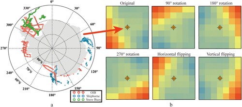
To address the relatively limited distribution of OIB snowpack measurements in East Antarctica, we incorporated snow depths from observations made during the 29th, 30th, and 31st Chinese National Antarctic Research Expeditions. These observational data were collected following the Antarctic Sea Ice Processes and Climate (ASPeCt) protocol and predominantly covered the East Antarctic and Ross Sea regions (Figure 1(a)). The dataset spans the years 2012–2015, covering the months from November to March each year. Typically, the vessel navigates through areas with relatively thin ice; thus, to mitigate the influence of SIC, we applied a threshold of greater than 75% SIC to filter the observational data (Shen, Ke, and Li 2022).

To further substantiate the precision of the snow depth retrieval model, we employed data from the Alfred Wegener Institute (AWI) snow buoy data (http://www.m-eereisportal.de). During the selection of buoy data, we executed a rigorous quality control process, opting for buoys that recorded data for a minimum of 100 days within the melting season. Our chosen buoys include 2013S8 (2013/7/9–2014/1/1), 2014S9 (2014/2/5–2015/9/12), 2016S31 (2016/1/16–2017/1/24), and 2016S38 (2016/1/15–2017/5/8). Each snow buoy was equipped with four independent sensors for snow depth measurement, covering an area of approximately 10 square meters. The accuracy of snow depth recorded by these sensors is estimated to be around 1 cm (Nicolaus et al. 2021). These buoys are predominantly situated in the Weddell Sea (Figure 1(a)). The average values obtained from the four sensors at each measurement point were utilized to represent the snow depth at that specific location.

To align the observed snow depth data (comprising OIB, shipborne, and snow buoy data) with the MWRI pixels, we projected these three datasets onto the NSIDC polar stereo grid. In accordance with the methodology of Beitsch, Kern, and Kaleschke (2015), we computed daily average snow depth measurements for the same day and within the same pixel for each of the three datasets. This yielded an average value to portray the snow depth for the corresponding pixel. Subsequently, the OIB and shipborne data were utilized for snow depth modeling and testing, serving as the training and test datasets, while snow buoy data were exclusively designated for model validation, constituting the validation dataset.

2.4. ICESat-2 freeboard

We utilized ICESat-2 freeboard data from the ICESat-2 ATL10 product (version 6), released by NSIDC (https://nsidc.org/data/atl10/versions/6). The ICESat-2 ATL10 product provides sea ice freeboard estimates within 10-kilometer segments, using local sea surface references derived from sea ice leads within each segment (Kwok et al. 2020). Its along-track resolution varies, with strong beams reaching approximately 10–200 m and weak beams ranging from 40 to 800 m (Shen, Ke, and Li 2022). The deviation of the total freeboards within the 10 km segment was assessed at approximately 2–4 cm based on the OIB data (Kwok et al. 2019a). These estimations were limited to segments with ice concentrations exceeding 50%, and the height samples must be at least 50 km from the coast to mitigate uncertainties related to coastal tides and ocean wave interference (Kwok et al. 2019b; Kwok et al. 2020). Given the limited availability of valid data in summer, we downloaded the ICESat-2 ATL10 product covering the spring seasons of 2019 through 2021 and acquired the roughness distribution by computing the standard deviation of the sea ice freeboard at a 100 km grid resolution (Markus et al. 2011). Subsequently, an analysis was conducted to examine the impact of sea ice roughness on snow thickness variations. Additionally, we computed the distribution of snow depth using the sea ice freeboard, as described by Kern and Ozsoy-Cicek (2016), to evaluate the precision of the snow depth measurements performed in this study.

3 Method

3.1. Data preprocessing

Previous studies have frequently employed direct estimations of snow depth through the utilization of passive microwave brightness temperature data. This approach is rooted in the belief that a robust relationship exists between snow depth and variations in distinct frequency bands of passive microwave data (Markus and Cavalieri 1998). However, the Antarctic snowscape manifests significant heterogeneity, posing a formidable challenge to the deduction of snow characteristics solely based on remote sensing observations (Webster et al. 2018). Therefore, considering the spatial distribution and physical changes of Antarctic snow, we attempted to enhance the accuracy of snow depth data using multi-source inputs and deep learning. The distribution of snow depth on sea ice is a dynamic phenomenon, as evidenced by previous research highlighting the myriad factors influencing snow depth. These factors encompass, but are not limited to SIC (Markus and Cavalieri 1998; Rostosky et al. 2018), sea ice type (Arndt et al. 2016; Li, Chen, and Guan 2019), geographical region (Kern and Ozsoy-Cicek 2016; Yan et al. 2023), air temperature (Comiso, Cavalieri, and Markus 2003; Nicolaus et al. 2021), wind speed (Leonard and Maksym 2011; Palm et al. 2011), snowfall (Petty et al. 2018), and rainfall (Haas, Thomas, and Bareiss 2001; Jeffries et al. 2001). In this study, we propose the following snow depth model: (1) $\mathrm{SD}=F(\mathrm{TB},\mathrm{GR},T,C,S)$(1) where SD represents snow depth, F(*) represents the retrieval function (in this study, CNN was used as the retrieval function), and the input parameters are described as follows:

(1)	TB represents the MWRI brightness temperature corrected using the open water tie point: (2) $T_{\mathrm{bice}}(\mathrm{vp})={\displaystyle \frac{T_b(\mathrm{vp})-(1-\mathrm{SIC})\times T_{\mathrm{bow}}(\mathrm{vp})}{\mathrm{SIC}}}$(2) where v represents the frequency band, p represents the polarization mode (V/H), $T_b(\mathrm{vp})$ represents the brightness temperature, $T_{\mathrm{bice}}$ represents the ice surface brightness temperature, $T_{\mathrm{bow}}(\mathrm{vp})$ is the open-water surface brightness temperature, and $\mathrm{SIC}$ is the sea ice concentration.
(2)	$\mathrm{GR}$ represents the gradient ratio of passive microwave data and is closely associated with changes in snow depth. The relationships (including RMSE and correlation coefficient) between measured data and different GRs are shown in Table 1. The results indicate that $\mathrm{GR}(V36,V18)$, $\mathrm{GR}(H36,H10)$, and $\mathrm{GR}(H18,H10)$ not only have strong correlation coefficients with the measured data but also exhibit excellent model accuracy, with RMSE values all less than 13.00 cm. Therefore, these three $\mathrm{GR}$ parameters were selected as inputs. The calculation equation for $\mathrm{GR}$ is as follows: (3) $\mathrm{GR}(\mathrm{vp}2,\mathrm{vp}1)={\displaystyle \frac{T_{\mathrm{bice}}(\mathrm{vp}2)-T_{\mathrm{bice}}(\mathrm{vp}1)}{T_{\mathrm{bice}}(\mathrm{vp}2)+T_{\mathrm{bice}}(\mathrm{vp}1)}}$(3)
(3)	G represents the geographical spatial information, including SIC, sea ice type, and region. Mei and Maksym (2020) found that regions with similar textures tend to have similar snow/ice ratios, suggesting that geospatial information could enhance snow depth estimates. SIC was calculated using MWRI data and the ASI algorithm (Zhao et al. 2022). As there are no mature and reliable sea ice-type data available for Antarctica, we used the average minimum sea ice concentration for the past ten years (SICmin) as a substitute. Different regions exhibit varying climatic conditions, which influence snow depth distribution. Therefore, we introduced regional templates. For ease of collaborative use with other data, a code was assigned to each region's grid: Weddell Sea West (WSW): 1; Weddell Sea East (WSE): 2; East Antarctic (EA, including the Indian Ocean and Pacific Ocean): 3; Ross Sea (RS): 4; and Bellingshausen-Amundsen Sea (BAS): 5 (Kern and Ozsoy-Cicek 2016).
(4)	C represents environmental information, including T2 m, WS, SF, and TP. The Antarctic snow–sea ice system is characterized by highly variable meteorological conditions in which heavy snowfall and synoptically driven thaw events occur year-round (Arndt et al. 2016; Massom, Drinkwater, and Haas 1997). Precipitation (snowfall) is a major contributor to snow accumulation, playing a crucial role in increasing snow depth (Petty et al. 2018). Warm weather causes snow to melt and thus leads to a decrease in snow depth. Wind-blown snow can alter the distribution of snow. Leads in the Antarctic may serve as a significant sink for wind-blown snow due to their prevalence and the high frequency of snowfall and wind events (Leonard and Maksym 2011).
(5)	S represents the polarization ratio between the SMOS 1.4 GHz vertical and horizontal brightness temperatures. The SMOS, operating at 1.4 GHz, offers enhanced penetration capabilities and effectively captures the characteristics of melting-season snow. In contrast to the gradient ratio between the SMOS and MWRI channels, utilizing the polarization ratio computed directly from the SMOS brightness temperature proved more beneficial for estimating snow depth (Braakmann-Folgmann and Donlon 2019). The equation for $\mathrm{PR}(1.4)$ is as follows: (4) $\mathrm{PR}(1.4)={\displaystyle \frac{T_b(1.4\mathrm{V})-T_b(1.4\mathrm{H})}{T_b(1.4\mathrm{V})+T_b(1.4\mathrm{H})}}$(4)

We individually standardized the different orders of magnitude of the input elements. Subsequently, we aggregated these elements centered on pixels corresponding to the measured snow depth data and divided them into windows of varying sizes for use as inputs to the CNN (window sizes: 3 × 3, 5 × 5, 7 × 7, and 9 × 9). The neural network input size was IW × IH × N, where IW and IH represent the width and height of the window, respectively, as determined by the window size, and N denotes the depth contingent on the number of input element types.

Table 1. The relationships (including RMSE and correlation coefficient) between measured data and different GRs.

GR	r	RMSE	GR	r	RMSE
GR(V89, V36)	−0.18	14.59	GR(H89, H36)	−0.10	14.74
GR(V89, V23)	−0.37	13.82	GR(H89, H23)	−0.27	14.3
GR(V89, V18)	−0.42	13.52	GR(H89, H18)	−0.32	14.07
GR(V89, V10)	−0.47	13.21	GR(H89, H10)	−0.41	13.58
GR(V36, V23)	−0.49	13.04	GR(H36, H23)	−0.48	13.09
GR(V36, V18)	−0.50	12.95	GR(H36, H18)	−0.49	13.05
GR(V36, V10)	−0.49	13.01	GR(H36, H10)	−0.52	12.80
GR(V23, V18)	−0.44	13.39	GR(H23, H18)	−0.40	13.67
GR(V23, V10)	−0.45	13.32	GR(H23, H10)	−0.48	13.08
GR(V18, V10)	−0.44	13.40	GR(H18, H10)	−0.51	12.90

3.2. Data enhancement

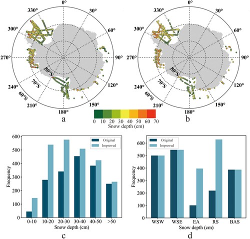
We randomly selected 70% of the measured snow depth data as the training dataset and allocated the remaining 30% to the test dataset. The spatial distributions of the training and test datasets are shown in Figures 2(a) and (b), respectively. Figure 2(c) and (d) display the data statistics of the training dataset for different numerical ranges and regions. The training dataset was not evenly distributed in space, particularly with relatively fewer measured data points in southeastern Antarctica and the Ross Sea. In terms of numerical distribution, there was a relative scarcity of records of shallow snow layers (<20 cm) in the training dataset. Such spatial and numerical imbalances could have adverse effects on neural network training. Given that shipborne observational data are primarily concentrated in the southeastern Antarctic and Ross Sea regions and typically record thinner snow layers, we applied data augmentation to the shipborne observational data in the training dataset. This augmentation included 90°, 180°, and 270° rotation, horizontal and vertical flipping (Figure 1(b)) (Cui et al. 2022). The results of the data augmentation are presented in Figure 2(c) and (d), revealing a significant increase in the number of records for shallow snow layers in the training dataset. Moreover, the training dataset exhibited a relatively balanced spatial distribution. Although augmented samples may not be entirely independent, data augmentation method contribute to diversifying the dataset. The model can better capture different aspects of the data, thereby improving its generalization capability. Ultimately, the training dataset comprises 2,458 snow depth data points, whereas the test dataset comprises 753 points.

Figure 2. The spatial distribution of the training (a) and test (b) datasets with the data statistics for the dataset in different numerical ranges (c) and regions (d).

3.3. Point-centered snow depth CNN

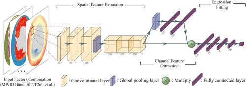
Considering the observation that regions with similar textures exhibit similar ice-to-snow ratios (Mei and Maksym 2020), we employed a Point-Centered Snow Depth CNN (PSDCNN) to retrieve snow depth on Antarctic sea ice using novel images composed of different input factors (Figure 3). CNN can learn to detect various patterns such as edges, textures, or shapes. The PSDCNN comprises three main components: spatial feature extraction, channel feature extraction, and regression fitting. The spatial feature extraction section encompasses six convolutional layers that automatically learn and extract spatial features from the input data by employing sliding convolution kernels to capture local information. The channel feature extraction section utilizes a channel attention module to adjust the importance of different channels (or feature maps). This aids the model in selecting the most relevant features for processing. The channel attention module includes a global pooling layer and two fully connected layers. The global pooling layer performs dimension reduction on the features extracted by the convolutional layers and then uses two fully connected layers to learn channel attention. Finally, the learned channel attention is applied to the original feature matrix through element-wise multiplication, weighting the features in the spatial dimension. Following channel feature extraction, the extracted features are flattened and passed through four fully connected layers for regression fitting. The number of neurons in these fully connected layers progressively decreases, with the final output layer containing only one neuron representing the estimated snow depth on Antarctic sea ice.

Figure 3. Convolutional neural network structure for snow depth estimation (input size is 7 × 7).

4. Results

4.1. Determination of optimal input parameters and window sizes for PSDCNN

Traditional models typically employ passive microwave brightness temperature data to estimate snow depth. To achieve a balance between the network complexity and the inclusion of the most informative predictors, we selected MWRI data from different channels and calculated the GR as the fundamental input parameter for the PSDCNN. Additional elements were gradually introduced, as outlined in Table 2. Simultaneously, we conducted experiments with various input window sizes and employed a test dataset to assess the model's accuracy. The random initialization of all learnable weights and biases at the start of training for the PSDCNN resulted in fluctuations to some extent in each training run. Each neural network underwent ten runs with different input parameters and window sizes, and the average was utilized to represent the accuracy of the model (Figure 4). We observed that accuracy progressively improved as the input size increased but reached a saturation point at an input window size of 7 × 7. Among the same input sizes, the 5th combination of input parameters performed the best, particularly at the 7 × 7 input window size (PSDCNN-5_7), where the model achieved the highest accuracy (Root Mean Square Error, RMSE: 7.24 cm). Compared to other factors, SIC, SICmin, and T2 m showed a closer association with the spatial distribution of snow depth. Including SIC, SICmin, and T2 m as part of the input data provides essential environmental context for the neural network, enhancing its understanding of the sea ice surface. Moreover, these environmental factors can reflect seasonal and geographical variations, further refining the accuracy of snow depth retrieval. Considering that the SMOS data do not cover the entire Antarctic region, we introduced SMOS data in the final stage of input parameter testing. The training dataset comprised only 1058 data points, and the test dataset comprised only 334 data points. With the addition of SMOS data to the PSDCNN-5_7 model (PSDCNN-SMOS), there was a slight improvement in the accuracy of the partial test dataset, yielding an RMSE of 7.15 cm.

Figure 4. Accuracy evaluations of PSDCNN with different input parameters and window sizes.

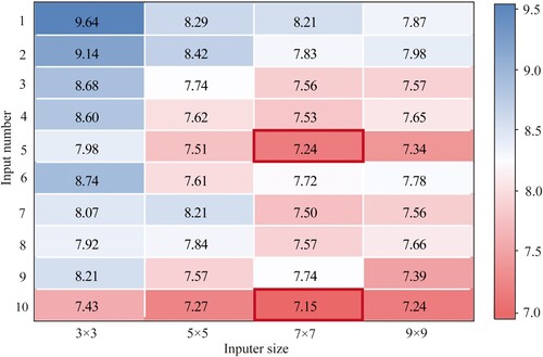
Table 2. Different input parameters used in this study to construct neural networks.

Input number	Input variables
1	MWRI bands, GR (V36, V18), GR (H36, H10), GR (H18, H10)
2	MWRI bands, GR (V36, V18), GR (H36, H10), GR (H18, H10), SIC
3	MWRI bands, GR (V36, V18), GR (H36, H10), GR (H18, H10), SIC, SICmin
4	MWRI bands, GR (V36, V18), GR (H36, H10), GR (H18, H10), SIC, SICmin, Place
5	MWRI bands, GR (V36, V18), GR (H36, H10), GR (H18, H10), SIC, SICmin, T2M
6	MWRI bands, GR (V36, V18), GR (H36, H10), GR (H18, H10), SIC, SICmin, Place, T2M
7	MWRI bands, GR (V36, V18), GR (H36, H10), GR (H18, H10), SIC, SICmin, T2M, WS
8	MWRI bands, GR (V36, V18), GR (H36, H10), GR (H18, H10), SIC, SICmin, T2M, SF
9	MWRI bands, GR (V36, V18), GR (H36, H10), GR (H18, H10), SIC, SICmin, T2M, TP
10 (5 + SMOS)	MWRI bands, GR (V36, V18), GR (H36, H10), GR (H18, H10), SIC, SICmin, T2M, SMOS

4.2. Evaluation of snow depth retrieval models

4.2.1. Comparison to the test dataset

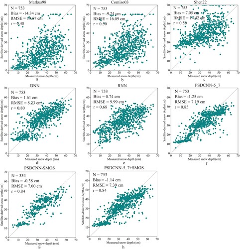
Six models, comprising traditional models (Markus98, Comiso03, and Shen22) and deep-learning models (DNN, RNN, and PSDCNN), underwent evaluation using the test dataset (Figure 5). Traditional models exhibited significantly lower accuracy compared to deep-learning models, possibly due to the latter’s superior ability to learn features from similar data during training. Among the traditional models, the Shen22 model demonstrated the highest accuracy, yielding an RMSE of 14.42 cm and a correlation coefficient of 0.50. This superiority can be attributed to the incorporation of OIB data into the Shen22 model. However, it tended to overestimate snow depth by 7.05 cm, particularly in shallow snow layers. All deep learning models displayed high accuracy on the test dataset. The RNN algorithm performed relatively poorly, registering an RMSE of 9.99 cm and a correlation coefficient of only 0.68. Given its primary design for handling sequential information, such as time-series problems, the RNN model may not be as effective for retrieval tasks. Notably, the PSDCNN-5_7 model showcased the best performance on the test dataset, boasting a bias of −1.25 cm, the lowest RMSE of 7.19 cm, and a correlation coefficient of 0.85. Due to incomplete coverage of the Antarctic region by SMOS data, only 334 points were available in the test dataset, significantly fewer than in other algorithms (753 points). The PSDCNN-SMOS model also exhibited good accuracy on the test dataset, with an RMSE of 7.00 cm. Attempts were made to combine both models (PSDCNN-5_7 + SMOS) using the snow depth estimated by the PSDCNN-5_7 model to fill gaps in the PSDCNN-SMOS model (Braakmann-Folgmann and Donlon 2019). However, the accuracy was lower than when using the PSDCNN-5_7 model alone, indicating that the PSDCNN-SMOS model did not surpass the performance of the PSDCNN-5_7 model. The introduction of SMOS data may not necessarily enhance the accuracy of snow depth models (Li et al. 2022).

Figure 5. Test dataset versus Markus98 (a), Comiso03 (b), Shen22 (c), DNN (d), RNN (e), PSDCNN-5_7 (f), PSDCNN-SMOS (g), and PSDCNN-5_7 + SMOS (h) models.

4.2.2. Comparison to the validation dataset

Figure 6 depicts the evaluation of six models, encompassing both traditional models (Markus98, Comiso03, and Shen22) and deep learning models (DNN, RNN, and PSDCNN), utilizing the validation dataset. Among the traditional models, the Shen22 model exhibited the poorest performance. Similar to the evaluation on the test dataset, the Shen22 model tended to overestimate snow depth in shallow layers, resulting in a bias of 10.59 cm and an RMSE of 17.37 cm. However, the remaining two traditional models consistently underestimated snow depth. Specifically, the Markus98 model displayed significant underestimation in deeper snow layers, with a bias of -8.30 cm. In contrast, the Comiso03 model performed the best among the traditional models, demonstrating an underestimation bias of -3.31 cm and an RMSE of 13.37 cm. The three deep-learning models consistently outperformed the traditional models on the validation dataset. The PSDCNN-5_7 model exhibited the highest accuracy, with a bias of −3.38 cm, an RMSE of 9.74 cm, and a correlation coefficient of 0.64. Table 3 demonstrates the comparison of the validation dataset with the Markus98, Comiso03, Shen22, DNN, RNN, and PSDCNN-5_7 models across different snow depth bins. We found that the Markus98 model delivers the best performance for shallow snow (<20 cm) with an RMSE of 4.61 cm, but performs poorly for deeper snow with an RMSE of 18.83 cm. This could be attributed to the model's reliance on ship-based measurements for its modeling, as ships typically avoid thick ice, leading to observations of thinner snow depths. The PSDCNN-5_7 model performs particularly well in estimating a medium-depth snow (20-40 cm) with an RMSE of 10.48 cm. All three deep learning models exhibit outstanding performance on deep snow (>40 cm). Specifically, the DNN model achieves the highest accuracy with an RMSE of just 6.34 cm, followed by the PSDCNN-5_7 model with an RMSE of 9.10 cm.

Figure 6. Validation dataset versus Markus98 (a), Comiso03 (b), Shen22 (c), DNN (d), RNN (e), PSDCNN-5_7 (f) models.

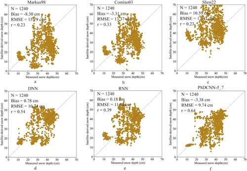
Table 3. Validation dataset versus Markus98, Comiso03, Shen22, DNN, RNN, and PSDCNN-5_7 models in different snow depth bins.

Model	<20 (cm)		20–40 (cm)		>40 (cm)
	Bias	RMSE	Bias	RMSE	Bias	RMSE
Markus98	3.11	4.61	−4.57	14.09	−14.89	18.83
Comiso03	8.61	9.27	0.09	12.8	−9.63	14.67
Shen22	24.51	24.83	16.14	24.12	3.78	12.63
DNN	5.71	6.85	2.59	14.04	−2.28	6.34
RNN	10.99	11.99	2.27	13.75	−4.46	9.26
PSDCNN-5_7	3.37	8.58	−2.72	10.48	−5.58	9.10

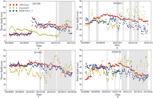
In prior assessments, the Comiso03 model demonstrated superior performance among conventional models. To comprehensively contrast the disparities between the traditional model and our proposed model, we analyzed their respective performances utilizing AWI buoy data across a time series (Figure 7). The gray shading in the figure denotes the snowmelt flag determined based on T2 m. Specifically, when the temperature at a given pixel surpasses −2°C, or when there are at least 5 days within the past 10 with temperatures exceeding this threshold, it is designated as a melting period (Rostosky et al. 2018). Comiso03 exhibits numerous inaccuracies when snowmelt occurs. The initiation of melting does not immediately translate to a reduction in snow depth. However, the traditional model displays a relatively high sensitivity, resulting in a significant underestimation of snow depth. In contrast, the snow depths estimated by the PSDCNN-5_7 model align well with those recorded by the AWI buoys. In summary, the PSDCNN-5_7 model outperformed both the test and validation datasets, establishing itself as an accurate, reliable, and effective method for snow depth detection.

Figure 7. Performance of Comiso03 and PSDCNN-5_7 models on the AWI buoy data: 2013S8 (a), 2016S31 (b), 2014S9 (c), and 2016S38 (d).

4.3. Differences in the spatial distributions of snow depth obtained by different models

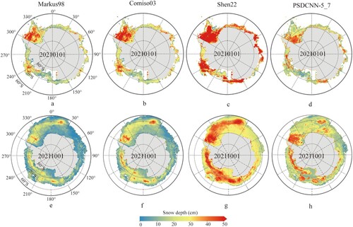
Figure 8 illustrates the spatial distribution of snow depth in the Antarctic austral spring (20211001) and summer (20210101), calculated using both the traditional model and the PSDCNN-5_7 model proposed in this study. Consistent with previous evaluation analyses, the traditional algorithms exhibited erroneous responses. In spring, both the Markus98 and Comiso03 models underestimated the snow depth in the Antarctic Peninsula and the Bellingshausen-Amundsen Sea, regions characterized by multiple years of ice with heavy snow cover. Although the Comiso03 model represented an improvement over the Markus98 model, it still exhibited a slight underestimation. In summer, the traditional models displayed severe overestimation. Specifically, the Shen22 model generated higher snow depth estimates, with values exceeding 30 cm for most of Antarctica. In contrast, the snow depth distribution derived from the PSDCNN-5_7 model was more reasonable.

Figure 8. The spatial distribution of snow depth in spring and summer calculated using the Markus98 (a), Comiso03 (b), Shen22 (c), and PSDCNN-5_7 models.

4.4. Variations in snow depth over Antarctic sea ice during melting seasons

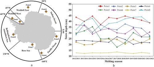
We utilized the PSDCNN-5_7 model to estimate snow depth on the sea ice surface during the melting season for each year from 2012 to 2022. Due to significant fluctuations in the extent of Antarctic sea ice during the melting season and substantial spatial variations in snow depth, the average snow depth in the sea area cannot accurately depict changes in snow depth (Li et al. 2022). Therefore, following the selection criteria based on Arndt et al. (2016), we obtained snow depth variations at eight points (each representing a pixel size and labeled as Point 1–8) during the melting season from 2012 to 2022 (Figure 9). Point 1, situated in the West Weddell Sea, exhibited the deepest snow, followed by Point 8, located along the coast of the Bellingshausen-Amundsen Sea. The snow depth in these two regions reached 40 cm, and a notable decline was observed during the 2015/2016 melting season. Additionally, Points 1 and 2 (Weddell Sea West) experienced a turning point in 2018/2019, with a recent continuous decrease in snow depth. Point 7 (Ross Sea) had the lowest snow depth, followed by Points 3 (Weddell Sea East) and 4 (Indian Ocean). Throughout the study period, the average snow depth in these regions remained relatively stable with minimal variation. However, the snow depth in most regions displayed a declining trend.

Figure 9. (a) Distribution of eight small regions in the Antarctic. (b) Variations in snow depth during the melting season from 2012 to 2022 in the eight small regions.

5. Discussion

5.1. Uncertainties, advantages, and limitations of the proposed PSDCNN-5_7 model

The proposed PSDCNN-5_7 model in this study is characterized as a complex nonlinear model. To assess its robustness, a Monte Carlo analysis, as elucidated by Liu et al. (2021) and Li et al. (2022), was undertaken. The Monte Carlo method entails continuous sampling and gradual approximation. Specifically, for each input value, we took the original input as the mean and the input uncertainty as the standard deviation. Subsequently, 50 data points were randomly sampled from a normal distribution to construct a dataset. For example, in the case of brightness temperature, the observed MWRI brightness temperature served as the mean, with a standard deviation of 0.5 K for MWRI. Subsequently, 50 brightness temperature samples were randomly drawn from a normal distribution. The uncertainties associated with SIC and SICmin were fixed at 5%. Using the Gaussian error propagation method, uncertainties in the GR were computed, yielding values of 0.0066 (GR(V36, V18)), 0.0082 (GR(H36, H10)), and 0.0034 (GR(H18, H10)). For T2 m, the daily standard deviation of T2 m temperatures over the study period was calculated, with the average serving as the uncertainty (0.3551 K). Each sample set was fed into the model, and the standard deviation of the output snow depth was computed as an indicator of snow depth uncertainty. The final uncertainty of the snow depth caused by the model input was determined to be 1.64 cm. This signifies the robustness of the PSDCNN-5_7 model, indicating minimal susceptibility to input data uncertainty and showcasing commendable noise resistance.

During snowmelt and refreezing, snow undergoes phase changes that lead to variations in microwave emissivity and penetration depth at its surface (Cavalieri et al. 2012; Zheng et al. 2020). Consequently, it becomes challenging to accurately depict the relationship between brightness temperature and snow depth using a fixed equation during the melting period. This limitation is a significant reason why traditional models struggle to precisely estimate snow depth during this phase. However, the approach proposed in this study not only capitalizes on the advantages of high- and low-frequency signals in snow depth retrieval but also integrates multiple geospatial and meteorological information features from various perspectives. This integration enhances the accuracy and stability of the model. However, toward the end of the melting season, surface snow may become highly rotten and deformed, making it no longer simple to consider as snow. Ice-on-snow precipitation can greatly change the thermal and optical properties of snow, such as increasing thermal conductivity and reducing albedo (Arndt et al. 2017). These changes increase the uncertainty in snow depth estimation.

The PSDCNN-5_7 model demonstrated notable accuracy; nevertheless, the efficacy of neural network models relied upon the precision and representativeness of the training data. Given that the training data for this study were acquired during the melting phase, the PSDCNN-5_7 model posited herein is better suited for the protracted estimation of snow depth on sea ice during the Antarctic melting season. Constrained by the extreme climate conditions of Antarctica, in-situ measurements of snow depth on Antarctic sea ice remain limited. With the acquisition of more in-situ data in the future, the algorithms can be further improved.

5.2. Comparison to ICESat-2 snow depth with sea ice roughness

The accuracy of the proposed snow depth estimation approach in this study was further assessed by comparing the spatial distribution of ICESat-2 snow depth with that of the traditional model (Comiso03 model) and the PSDCNN-5_7 model (Figure 10). The spatial distribution of snow depth estimated by the PSDCNN-5_7 model exhibited a high degree of consistency with the ICESat-2 snow depth from September to November. However, the traditional model displayed severe underestimation in many regions, particularly in the West Weddell Sea, Bellingshausen–Amundsen Sea, and along the coast of East Antarctica. The distribution of snow depth on Antarctic sea ice is closely related to the ice age and surface roughness (Jeffries et al. 2001). These areas are characterized by multiyear ice, which inherently contains deep snow. In the early phases of snowmelt, there is no immediate reduction in snow depth because the prior snow layer is compacted (Arndt et al. 2016). The traditional model is highly sensitive to snowmelt, which may be one reason for the underestimation of snow depth (Comiso, Cavalieri, and Markus 2003; Markus and Cavalieri 1998). Additionally, we found that the areas underestimated by the traditional models aligned well with areas of high ice roughness. This also demonstrated that the traditional model provided relatively accurate estimates of snow depth for smooth sea ice but significantly underestimated snow depth for deformed (rough) sea ice, with underestimations of up to 2–4 times (Kern et al. 2011; Worby et al. 2008).

Figure 10. Spatial distribution of snow depth estimated by PSDCNN-5_7 model (a) and Comiso03 model (b), ICESat-2 snow depth (c), and sea ice roughness (d). Difference denotes November minus September.

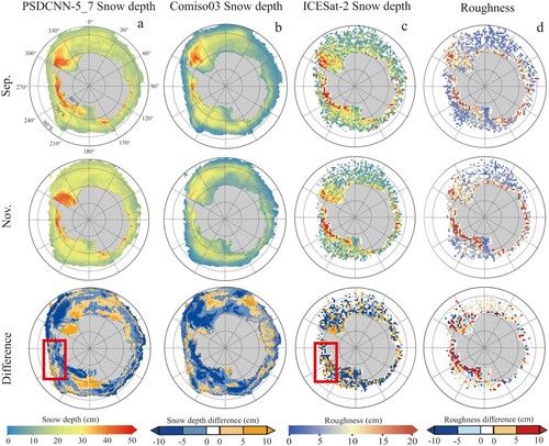
Although the PSDCNN-5_7 model exhibited a high degree of spatial consistency with ICESat-2 snow depth, we did not observe an increasing trend in the PSDCNN-5_7 model snow depth in the coastal areas of the Bellingshausen-Amundsen Sea. Comparing variations in sea ice roughness, we found a significant increase in roughness from September to November in the Antarctic Peninsula and the coastal regions of the Bellingshausen-Amundsen Sea. This increase may be associated with melting ice and intense meteorological activity during the melting season. Furthermore, ICESat-2 snow depth increases with increasing ice roughness. This phenomenon can be attributed to two factors. First, the rough sea ice surface facilitates snow accumulation, and the higher annual precipitation in the western Antarctic region may locally increase snow depth (Maksym and Markus 2008). Second, the ICESat-2 snow depth retrieval algorithm is sensitive to the surface characteristics of sea ice, particularly the ice freeboard. Therefore, during the melting season, ICESat-2 may have an easier time identifying snow on deformed sea ice, resulting in the overestimation of snow depth (Kern and Ozsoy-Çiçek 2016). The high consistency in the temporal and spatial distribution of snow depth between this study and ICESat-2 further demonstrates the reliability of the snow depth approach proposed in this study.

5.3. Relationships between snow depth and SIC, SIA, T2 m, SF, TP, WS, SIV

Snow depth is highly sensitive to the SIC, sea ice area (SIA), T2 m, SF, TP, WS, and SIV (Knuth et al. 2010; Petty et al. 2018). Therefore, we conducted correlation to examine the relationships between snow depth in different Antarctic seas and environmental factors (Table 4). To ensure that the analysis was not influenced by temporal trends, we detrended the data before conducting the correlation analysis. During the melting season in West Antarctica, variations in snow depth were primarily positively correlated with SIC. In East Antarctica, snow depth exhibited a notable dependence on SIA and SIV, demonstrating a discernible negative correlation. As SIA and SIV decreased, there was a corresponding increase in average snow depth. This phenomenon may be attributed to the persistence of multi-year ice with deeper snow layers after the complete seasonal ice melt. This residual ice contributes to the average elevation of snow depth in the region.

Table 4. Correlation analysis between snow depths of different seas and SIC, SIA, T2 m, SF, TP, WS, and SIV during the melting season.

Factor	Weddell Sea West	Weddell Sea East	Ross Sea	Bellingshausen-Amundsen Sea	Indian Ocean	Pacific Ocean
SIC	0.48**	0.69**	0.46**	0.46**	−0.28*	−0.28*
SIA	−0.14	0.47**	0.37**	0.24	−0.61**	−0.78**
T2m	0.10	−0.58**	−0.51**	−0.31*	0.36**	0.70**
SF	0.20	0.61**	0.42**	0.38**	−0.24	−0.34**
TP	0.01	0.26*	−0.12	−0.18	−0.13	0.52**
WS	−0.09	0.52**	0.26*	0.23	−0.43**	−0.57**
SIV	−0.10	0.41**	0.16	0.13	−0.78**	−0.84**

Note: (* denotes p < 0.05; ** denotes p < 0.01).

Table 5 showed that multiple GLM analysis between snow depths of different seas and T2 m, SF, TP, WS, and SIV during the melting season. In the multiple GLM analysis, we employed a backward stepwise procedure to determine the best-fit model and used Analysis of Variance (ANOVA) to obtain the proportion of explained variance (SS) of the independent variables in the model, indicating the contribution of environmental factors to snow depth variations. In West Antarctica, variations in snow depth are primarily driven by three key factors: SF, T2 m and SIV. SF contributes to a rise in snow depth. The West Antarctic area is known for frequent cyclone activity and thus higher snowfall rates (Markus and Cavalieri 2006). Conversely, rising T2 m and sea ice drift predominantly lead to a decrease in snow depth. Specifically, in the Weddell Sea East, these factors collectively explain 97.23% of the changes in snow depth. As temperatures rise and snowfall diminishes throughout the melting season, snow depth undergoes a gradual reduction. Sea ice drift leads to a portion of the sea ice moving towards lower latitudes, accelerating the melting of the snow. Another part of the sea ice is transported clockwise within the cyclonic gyre into the Western Weddell Sea (Kacimi and Kwok 2020). In the Ross Sea, a combination of factors affects snow depth changes. However, T2 m and SIV are predominant, accounting for 66.94% of the variations in snow depth. T2 m primarily controls snowmelt, and in the summer, the area near the Ross Ice Shelf doesn't even have sea ice and snow. The Ross Shelf Polynya, along with the Terra Nova Bay and McMurdo Sound polynya regions, are significant zones for new ice production. Driven by cyclones, numerous inter-ice shelf polynyas generate a substantial amount of first-year ice with relatively thinner snow, which subsequently drifts towards lower latitudes (Comiso et al. 2011; Kacimi and Kwok 2020). Half of the sea ice in the Ross Sea is produced within wind-sustained latent-heat polynyas (Mezgec et al. 2017), resulting in generally thinner snow depth in the Ross Sea. Moreover, drift patterns (Figure 11) indicate that thicker sea ice flows into the Ross Sea from the eastern Amundsen Sea coast, with its thickness notably greater than the thinner ice exiting from the southern Ross Sea. This thicker ice also typically carries a thicker snow cover, elevating the average snow depth in the Ross Sea. Snow in the Weddell Sea West and the Bellingshausen-Amundsen Sea is particular in that it typically survives summer ablation. Compaction and evaporation have a greater impact on snow thinning in the Weddell Sea west than melting (Nicolaus, Haas, and Willmes 2009). Additionally, the direction of sea ice drift changes significantly over time. SF contributes significantly to snow depth across these regions. In East Antarctica, the variation in snow depth is primarily driven by sea ice drift. In contrast to the intricate topography of West Antarctica, East Antarctica boasts a more straightforward landscape and borders the expansive Pacific and Indian Oceans, where sea ice movement predominantly follows a divergent pattern (Heil et al. 2001). As the sea ice drifts towards lower latitudes, the snow becomes exposed to progressively warmer waters, leading to gradual melting.

Figure 11. The sea ice velocities during the melting season. The black arrow represents the direction of sea ice motion.

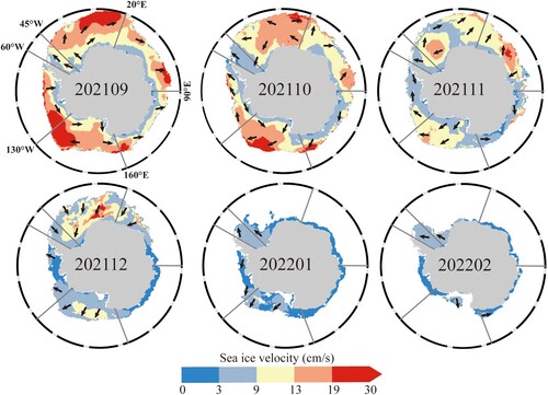
Table 5. Multiple GLM analysis between snow depths of different seas and T2 m, SF, TP, WS, and SIV during the melting season.

Factor	Weddell Sea West	Weddell Sea East	Ross Sea	Bellingshausen-Amundsen Sea	Indian Ocean	Pacific Ocean
T2m	/	28.18**	35.70**	/	1.57	/
SF	52.33	44.63**	14.21*	55.13**	6.82**	10.64**
TP	/	/	5.72	12.25*	/	/
WS	34.43	/	10.76*	/	/	/
SIV	/	24.42**	31.24**	29.59**	91.01**	88.75**
Residuals	13.24	2.77	2.38	3.03	0.93	0.61

Note: (* denotes p < 0.05; ** denotes p < 0.01).

6. Conclusions

This study integrated multiple data, including satellite remote sensing, geospatial information, and meteorological data. Subsequently, a CNN was employed to extract spatial and channel features and perform regression fitting to construct a snow depth retrieval model (PSDCNN-5_7 model). Among the six models (three traditional models and three deep learning models), PSDCNN-5_7 exhibited the highest accuracy, with a RMSE of 7.19 cm on the test dataset. When compared to snow depth measurements from AWI snow buoys, the PSDCNN-5_7 model exhibited a bias of -3.38 cm and an RMSE of 9.74 cm. The PSDCNN-5_7 model demonstrates robustness with minimal susceptibility to uncertainties in the input data. Monte Carlo testing indicates that the uncertainty of the snow depth caused by the model input is only 1.64 cm.

The PSDCNN-5_7 model was employed to estimate snow depth on Antarctic sea ice during the melting season from 2012 to 2022. Most regions of the Antarctic Ocean exhibit a decreasing trend in snow depth. The West Weddell Sea exhibited the highest snow depth, with an average snow depth of 40 cm. However, there has been a continuous decline in snow depth in the West Weddell Sea in recent years. In contrast, the Ross Sea had the lowest snow depth and remained relatively stable throughout the study period, with minimal variation. The snow depth derived from PSDCNN-5_7 is closely aligned with the heights obtained from ICESat-2 snow depth. Conversely, traditional models display numerous inaccuracies, particularly underestimation of snow depth in the West Weddell Sea, Bellingshausen-Amundsen Sea, and along the coastal areas of the East Antarctic.

Variations in snow depth in Antarctic sea ice in different regions are influenced by multiple environmental factors, with varying dominant factors in different sea areas. During the melting season in West Antarctica, snow depth is affected more by SF, T2 m, and SIV. Specifically, in the Weddell Sea East, these factors collectively explain 97.23% of the changes in snow depth. In contrast, in East Antarctica, snow depth is primarily influenced by SIV. However, the environmental factors discussed in this study were limited. In the future, we will integrate additional environmental data and delve deeper into the mechanisms driving variations in snow depth on Antarctic sea ice. Because field measurements of snow depth were primarily concentrated in West Antarctica, we intend to enhance in situ measurements of snow on East Antarctic sea ice in the future and establish a long-term monitoring system to track variations in snow depth on Antarctic sea ice.

Acknowledgements

We thank the members of the 29th, 30th, and 31st Chinese National Antarctic Research Expedition and the crews of R/V Xuelong for their assistance during snow depth observations.

Disclosure statement

No potential conflict of interest was reported by the author(s).

Data availability statement

The data that support the findings of this study are available from the corresponding author, upon reasonable request.

Additional information

Funding

This work was supported by the National Natural Science Foundation of China [grant number: 42076235] and the Fundamental Research Funds for the Central Universities [grant number: 2042022dx0001].

References

- Arndt, S., K. M. Meiners, R. Ricker, T. Krumpen, C. Katlein, and M. Nicolaus. 2017. “Influence of Snow Depth and Surface Flooding on Light Transmission Through Antarctic Pack Ice.” Journal of Geophysical Research: Oceans 122 (3): 2108–2119. https://doi.org/10.1002/2016JC012325.
- Arndt, S., S. Willmes, W. Dierking, and M. Nicolaus. 2016. “Timing and Regional Patterns of Snowmelt on Antarctic Sea Ice from Passive Microwave Satellite Observations.” Journal of Geophysical Research: Oceans 121 (8): 5916–5930. https://doi.org/10.1002/2015JC011504.
- Beitsch, A., S. Kern, and L. Kaleschke. 2015. “Comparison of SSM/I and AMSR-E Sea Ice Concentrations with ASPeCt Ship Observations Around Antarctica.” IEEE Transactions on Geoscience and Remote Sensing 53 (4): 1985–1996. https://doi.org/10.1109/TGRS.2014.2351497.
- Blazey, B. A., M. M. Holland, and E. C. Hunke. 2013. “Arctic Ocean Sea Ice Snow Depth Evaluation and Bias Sensitivity in CCSM.” The Cryosphere 7 (6): 1887–1900. https://doi.org/10.5194/tc-7-1887-2013.
- Braakmann-Folgmann, A., and C. Donlon. 2019. “Estimating Snow Depth on Arctic Sea Ice Using Satellite Microwave Radiometry and a Neural Network.” The Cryosphere 13 (9): 2421–2438. https://doi.org/10.5194/tc-13-2421-2019.
- Cavalieri, D. J., T. Markus, A. Ivanoff, J. A. Miller, L. Brucker, M. Sturm, J. A. Maslanik, et al. 2012. “A Comparison of Snow Depth on Sea Ice Retrievals Using Airborne Altimeters and an AMSR-E Simulator.” IEEE Transactions on Geoscience and Remote Sensing 50 (8): 3027–3040. https://doi.org/10.1109/TGRS.2011.2180535.
- Chen, Y., R. Lei, X. Zhao, S. Wu, Y. Liu, P. Fan, Q. Ji, P. Zhang, and X. Pang. 2023. “A New Sea Ice Concentration Product in the Polar Regions Derived from the FengYun-3 MWRI Sensors.” Earth System Science Data 15 (7): 3223–3242. https://doi.org/10.5194/essd-15-3223-2023.
- Chen, Y., X. Zhao, X. P. Pang, and Q. Ji. 2022. “Daily Sea Ice Concentration Product Based on Brightness Temperature Data of FY-3D MWRI in the Arctic.” Big Earth Data 6 (2): 164–178. https://doi.org/10.1080/20964471.2020.1865623.
- Comiso, J. C., D. J. Cavalieri, and T. Markus. 2003. “Sea Ice Concentration, Ice Temperature, and Snow Depth Using AMSR-E Data.” IEEE Transactions on Geoscience and Remote Sensing 41 (2): 243–252. https://doi.org/10.1109/TGRS.2002.808317.
- Comiso, J. C., R. Kwok, S. Martin, and A. L. Gordon. 2011. “Variability and Trends in Sea Ice Extent and Ice Production in the Ross Sea.” Journal of Geophysical Research 116 (C4): C04021. https://doi.org/10.1029/2010JC006391.
- Cui, Y. H., Z. N. Yan, J. Wang, S. Hao, and Y. C. Liu. 2022. “Deep Learning–Based Remote Sensing Estimation of Water Transparency in Shallow Lakes by Combining Landsat 8 and Sentinel 2 Images.” Environmental Science and Pollution Research 29 (3): 4401–4413. https://doi.org/10.1007/s11356-021-16004-9.
- Fan, T. T., C. Deser, and D. P. Schneider. 2014. “Recent Antarctic Sea Ice Trends in the Context of Southern Ocean Surface Climate Variations Since 1950.” Geophysical Research Letters 41 (7): 2419–2426. https://doi.org/10.1002/2014GL059239.
- Fons, S. W., and N. T. Kurtz. 2019. “Retrieval of Snow Freeboard of Antarctic Sea Ice Using Waveform Fitting of CryoSat-2 Returns.” The Cryosphere 13 (3): 861–878. https://doi.org/10.5194/tc-13-861-2019.
- Haas, C., D. N. Thomas, and J. Bareiss. 2001. “Surface Properties and Processes of Perennial Antarctic Sea Ice in Summer.” Journal of Glaciology 47 (159): 613–625. https://doi.org/10.3189/172756501781831864.
- Heil, P., C. W. Fowler, J. A. Maslanik, W. J. Emery, and I. A. Allison. 2001. “A Comparison of East Antarctic Sea-Ice Motion Derived Using Drifting Buoys and Remote Sensing.” Annals of Glaciology 33: 139–144. https://doi.org/10.3189/172756401781818374.
- Jeffries, M. O., H. R. Krouse, B. Hurst-Cushing, and T. Maksym. 2001. “Snow-Ice Accretion and Snow-Cover Depletion on Antarctic First-Year Sea-Ice Floes.” Annals of Glaciology 33: 51–60. https://doi.org/10.3189/172756401781818266.
- Kacimi, S., and R. Kwok. 2020. “The Antarctic Sea Ice Cover from ICESat-2 and CryoSat-2: Freeboard, Snow Depth, and Ice Thickness.” The Cryosphere 14 (12): 4453–4474. https://doi.org/10.5194/tc-14-4453-2020.
- Kern, S., K. Khvorostovsky, H. Skourup, E. Rinne, Z. S. Parsakhoo, V. Djepa, P. Wadhams, and S. Sandven. 2015. “The Impact of Snow Depth. Snow Density and Ice Density on Sea Ice Thickness Retrieval from Satellite Radar Altimetry: Results from the ESA-CCI Sea Ice ECV Project Round Robin Exercise.” The Cryosphere 9 (1): 37–52. https://doi.org/10.5194/tc-9-37-2015.
- Kern, S., and B. Ozsoy-Çiçek. 2016. “Satellite Remote Sensing of Snow Depth on Antarctic Sea Ice: An Inter-Comparison of Two Empirical Approaches.” Remote Sensing 8 (6): 450. https://doi.org/10.3390/rs8060450.
- Kern, S., B. Ozsoy-Cicek, S. Willmes, M. Nicolaus, C. Haas, and S. Ackley. 2011. “An Intercomparison Between AMSR-E Snow-Depth and Satellite C- and Ku-Band Radar Backscatter Data for Antarctic Sea Ice.” Annals of Glaciology 52 (57): 279–290. https://doi.org/10.3189/172756411795931750.
- Kern, S., and B. Ozsoy. 2019. “An Attempt to Improve Snow Depth Retrieval Using Satellite Microwave Radiometry for Rough Antarctic Sea Ice.” Remote Sensing 11 (19): 2323. https://doi.org/10.3390/rs11192323.
- Kern, S., and G. Spreen. 2015. “Uncertainties in Antarctic Sea-Ice Thickness Retrieval from ICESat.” Annals of Glaciology 56 (69): 107–119. https://doi.org/10.3189/2015AoG69A736.
- Knuth, S. L., G. J. Tripoli, J. E. Thom, and G. A. Weidner. 2010. “The Influence of Blowing Snow and Precipitation on Snow Depth Change Across the Ross Ice Shelf and Ross Sea Regions of Antarctica.” Journal of Applied Meteorology and Climatology 49 (6): 1306–1321. https://doi.org/10.1175/2010JAMC2245.1.
- Kwok, R., S. Kacimi, T. Markus, N. T. Kurtz, M. Studinger, J. G. Sonntag, S. S. Manizade, L. N. Boisvert, and J. P. Harbeck. 2019a. “ICESat-2 Surface Height and Sea Ice Freeboard Assessed with ATM Lidar Acquisitions from Operation IceBridge.” Geophysical Research Letters 46 (20): 11228–11236. https://doi.org/10.1029/2019GL084976.
- Kwok, R., S. Kacimi, M. A. Webster, N. T. Kurtz, and A. A. Petty. 2020. “Arctic Snow Depth and Sea Ice Thickness from ICESat-2 and CryoSat-2 Freeboards: A First Examination.” Journal of Geophysical Research: Oceans 125 (3): e2019JC016008. https://doi.org/10.1029/2019JC016008.
- Kwok, R., T. Markus, N. T. Kurtz, A. A. Petty, T. A. Neumann, S. L. Farrell, G. F. Cunningham, D. W. Hancock, A. Ivanoff, and J. T. Wimert. 2019b. “Surface Height and Sea Ice Freeboard of the Arctic Ocean from ICESat-2: Characteristics and Early Results.” Journal of Geophysical Research: Oceans 124 (10): 6942–6959. https://doi.org/10.1029/2019JC015486.
- Leonard, K., and T. Maksym. 2011. “The Importance of Wind-Blown Snow Redistribution to Snow Accumulation on Bellingshausen Sea Ice.” Annals of Glaciology 52 (57): 271–278. https://doi.org/10.3189/172756411795931651.
- Li, L., H. Chen, and L. Guan. 2019. “Retrieval of Snow Depth on Sea Ice in the Arctic Using the FengYun-3B Microwave Radiation Imager.” Journal of Ocean University of China 18 (3): 580–588. https://doi.org/10.1007/s11802-019-3873-y.
- Li, H. L., C. Q. Ke, Q. Zhu, M. Li, and X. Shen. 2022. “A Deep Learning Approach to Retrieve Cold-Season Snow Depth Over Arctic Sea Ice from AMSR2 Measurements.” Remote Sensing of Environment 269: 112840. https://doi.org/10.1016/j.rse.2021.112840.
- Lindsay, R., and A. Schweiger. 2015. “Arctic Sea Ice Thickness Loss Determined Using Subsurface, Aircraft, and Satellite Observations.” The Cryosphere 9 (1): 269–283. https://doi.org/10.5194/tc-9-269-2015.
- Liu, H. Z., Q. Q. Li, Y. Bai, C. Yang, J. J. Wang, Q. M. Zhou, S. B. Hu, T. Z. Shi, X. M. Liao, and G. F. Wu. 2021. “Improving Satellite Retrieval of Oceanic Particulate Organic Carbon Concentrations Using Machine Learning Methods.” Remote Sensing of Environment 256: 112316. https://doi.org/10.1016/j.rse.2021.112316.
- Maksym, T. 2019. “Arctic and Antarctic Sea Ice Change: Contrasts, Commonalities, and Causes.” Annual Review of Marine Science 11 (1): 187–213. https://doi.org/10.1146/annurev-marine-010816-060610.
- Maksym, T., and T. Markus. 2008. “Antarctic Sea Ice Thickness and Snow-to-Ice Conversion from Atmospheric Reanalysis and Passive Microwave Snow Depth.” Journal of Geophysical Research: Oceans 113 (C2), https://doi.org/10.1029/2006JC004085.
- Marcianesi, F., G. Aulicino, and P. Wadhams. 2021. “Arctic Sea Ice and Snow Cover Albedo Variability and Trends During the Last Three Decades.” Polar Science 28: 100617. https://doi.org/10.1016/j.polar.2020.100617.
- Markus, T., and D. J. Cavalieri. 1998. Antarctic Sea Ice: Physical Processes, Interactions and Variability: Snow Depth Distribution Over Sea Ice in the Southern Ocean from Satellite Passive Microwave Data. Washington, USA: American Geophysical Union.
- Markus, T., and D. J. Cavalieri. 2006. “Interannual and Regional Variability of Southern Ocean Snow on Sea Ice.” Annals of Glaciology 44: 53–57. https://doi.org/10.3189/172756406781811475.
- Markus, T., D. J. Cavalieri, A. J. Gasiewski, M. Klein, J. A. Maslanik, D. C. Powell, B. B. Stankov, J. C. Stroeve, and M. Sturm. 2006. “Microwave Signatures of Snow on Sea Ice: Observations.” IEEE Transactions on Geoscience and Remote Sensing 44 (11): 3081–3090. https://doi.org/10.1109/TGRS.2006.883134.
- Markus, T., R. Massom, A. Worby, V. Lytle, N. Kurtz, and T. Maksym. 2011. “Freeboard, Snow Depth and Sea-Ice Roughness in East Antarctica from In Situ and Multiple Satellite Data.” Annals of Glaciology 52 (57): 242–248. https://doi.org/10.3189/172756411795931570.
- Markus, T., D. C. Powell, and J. R. Wang. 2006. “Sensitivity of Passive Microwave Snow Depth Retrievals to Weather Effects and Snow Evolution.” IEEE Transactions on Geoscience and Remote Sensing 44 (1): 68–77. https://doi.org/10.1109/TGRS.2005.860208.
- Maslanik, J. A., M. Sturm, M. B. Rivas, A. J. Gasiewski, J. F. Heinrichs, U. C. Herzfeld, J. Holmgren, et al. 2006. “Spatial Variability of Barrow-Area Shore-Fast Sea Ice and Its Relationships to Passive Microwave Emissivity.” IEEE Transactions on Geoscience and Remote Sensing 44 (11): 3021–3031. https://doi.org/10.1109/TGRS.2006.879557.
- Massom, R. A., M. R. Drinkwater, and C. Haas. 1997. “Winter Snow Cover on Sea Ice in the Weddell Sea.” Journal of Geophysical Research: Oceans 102 (C1): 1101–1117. https://doi.org/10.1029/96JC02992.
- Massom, R. A., H. Eicken, C. Hass, M. O. Jeffries, M. R. Drinkwater, M. Sturm, A. P. Worby, et al. 2001. “Snow on Antarctic Sea Ice.” Reviews of Geophysics 39 (3): 413–445. https://doi.org/10.1029/2000RG000085.
- Mei, M. J., and T. A. Maksym. 2020. “Textural Approach to Improving Snow Depth Estimates in the Weddell Sea.” Remote Sensing 12 (9): 1494. https://doi.org/10.3390/rs12091494.
- Mezgec, K., B. Stenni, X. Crosta, V. Masson-Delmotte, C. Baroni, M. Braida, V. Ciardini, et al. 2017. “Holocene Sea Ice Variability Driven by Wind and Polynya Efficiency in the Ross Sea.” Nature Communications 8: 1334. https://doi.org/10.1038/s41467-017-01455-x.
- Nicolaus, M., C. Haas, and S. Willmes. 2009. “Evolution of First-Year and Second-Year Snow Properties on Sea Ice in the Weddell Sea During Spring-Summer Transition.” Journal of Geophysical Research: Atmospheres 114: D17109. https://doi.org/10.1029/2008JD011227.
- Nicolaus, M., M. Hoppmann, S. Arndt, S. Hendricks, C. Katlein, A. Nicolaus, L. Rossmann, M. Schiller, and S. Schwegmann. 2021. “Snow Depth and Air Temperature Seasonality on Sea Ice Derived from Snow Buoy Measurements.” Frontiers in Marine Science 8: 655446. https://doi.org/10.3389/fmars.2021.655446.
- Palm, S. P., Y. Yang, J. D. Spinhirne, and A. Marshak. 2011. “Satellite Remote Sensing of Blowing Snow Properties Over Antarctica.” Journal of Geophysical Research 116: D16123. https://doi.org/10.1029/2011JD015828.
- Petty, A. A., M. Webster, L. Boisvert, and T. Markus. 2018. “The NASA Eulerian Snow on Sea Ice Model (NESOSIM) v1.0: Initial Model Development and Analysis.” Geoscientific Model Development 11 (11): 4577–4602. https://doi.org/10.5194/gmd-11-4577-2018.
- Powell, D. C., T. Markus, D. J. Cavalieri, A. J. Gasiewski, M. Klein, J. A. Maslanik, J. C. Stroeve, and M. Sturm. 2006. “Microwave Signatures of Snow on Sea Ice: Modeling.” IEEE Transactions on Geoscience and Remote Sensing 44 (11): 3091–3102. https://doi.org/10.1109/TGRS.2006.882139.
- Purich, A., and E. W. Doddridge. 2023. “Record Low Antarctic Sea Ice Coverage Indicates a New Sea Ice State.” Communications Earth & Environment 4 (1): 314. https://doi.org/10.1038/s43247-023-00961-9.
- Riihelä, A., R. M. Bright, and K. Anttila. 2021. “Recent Strengthening of Snow and Ice Albedo Feedback Driven by Antarctic Sea-Ice Loss.” Nature Geoscience 14 (11): 832–836. https://doi.org/10.1038/s41561-021-00841-x.
- Rostosky, P., G. Spreen, S. L. Farrell, T. Frost, G. Heygster, and C. Melsheimer. 2018. “Snow Depth Retrieval on Arctic Sea Ice from Passive Microwave Radiometers—Improvements and Extensions to Multiyear Ice Using Lower Frequencies.” Journal of Geophysical Research: Oceans 123 (10): 7120–7138. https://doi.org/10.1029/2018JC014028.
- Shen, X., C. Q. Ke, and H. Li. 2022. “Snow Depth Product Over Antarctic Sea Ice from 2002 to 2020 Using Multisource Passive Microwave Radiometers.” Earth System Science Data 14 (2): 619–636. https://doi.org/10.5194/essd-14-619-2022.
- Simmonds, I. 2015. “Comparing and Contrasting the Behaviour of Arctic and Antarctic Sea Ice Over the 35 Year Period 1979–2013.” Annals of Glaciology 56 (69): 18–28. https://doi.org/10.3189/2015AoG69A909.
- Simmonds, I., and K. Keay. 2000. “Mean Southern Hemisphere Extratropical Cyclone Behavior in the 40-Year NCEP–NCAR Reanalysis.” Journal of Climate 13 (5): 873–885.
- Simpkins, G. 2023. “Record Low Antarctic Sea Ice Extent.” Nature Reviews Earth & Environment 4 (5): 296. https://doi.org/10.1038/s43017-023-00433-w.
- Stroeve, J. C., T. Markus, J. A. Maslanik, D. J. Cavalieri, A. J. Gasiewski, J. F. Heinrichs, J. Holmgren, D. K. Perovich, and M. Sturm. 2006. “Impact of Surface Roughness on AMSR-E Sea Ice Products.” IEEE Transactions on Geoscience and Remote Sensing 44 (11): 3103–3117. https://doi.org/10.1109/TGRS.2006.880619.
- Trujillo, E., K. Leonard, T. Maksym, and M. Lehning. 2016. “Changes in Snow Distribution and Surface Topography Following a Snowstorm on Antarctic Sea Ice.” Journal of Geophysical Research: Earth Surface 121 (11): 2172–2191. https://doi.org/10.1002/2016JF003893.
- Webster, M., S. Gerland, M. Holland, E. Hunke, R. Kwok, O. Lecomte, R. Massom, D. Perovich, and M. Sturm. 2018. “Snow in the Changing Sea-Ice Systems.” Nature Climate Change 8 (11): 946–953. https://doi.org/10.1038/s41558-018-0286-7.
- Webster, M. A., I. G. Rigor, S. V. Nghiem, N. T. Kurtz, S. L. Farrell, D. K. Perovich, and M. Sturm. 2014. “Interdecadal Changes in Snow Depth on Arctic Sea Ice.” Journal of Geophysical Research: Oceans 119 (8): 5395–5406. https://doi.org/10.1002/2014JC009985.
- Wever, N., K. Leonard, T. Maksym, S. White, M. Proksch, and J. Lenaerts. 2021. “Spatially Distributed Simulations of the Effect of Snow on Mass Balance and Flooding of Antarctic Sea Ice.” Journal of Glaciology 67 (266): 1055–1073. https://doi.org/10.1017/jog.2021.54.
- Worby, A. P., T. Markus, A. D. Steer, V. I. Lytle, and R. A. Massom. 2008. “Evaluation of AMSR-E Snow Depth Product Over East Antarctic Sea Ice Using in Situ Measurements and Aerial Photography.” Journal of Geophysical Research: Oceans 113 (C5): C05S–C094. https://doi.org/10.1029/2007JC004181.
- Yan, Z. N., X. P. Pang, Q. Ji, Y. Z. Chen, C. X. Luo, P. Fan, and Z. Y. Liang. 2023. “Retrieval of Snow Depth on Antarctic Sea Ice from the FY-3D MWRI Data.” Acta Oceanologica Sinica 42 (12): 105–117. https://doi.org/10.1007/s13131-023-2179-5.
- Zhao, X., Y. Chen, S. Kern, M. Qu, Q. Ji, P. Fan, and Y. Liu. 2022. “Sea Ice Concentration Derived from FY-3D MWRI and Its Accuracy Assessment.” IEEE Transactions on Geoscience and Remote Sensing 60: 1. https://doi.org/10.1109/TGRS.2021.3063272.
- Zheng, L., C. Zhou, T. Zhang, Q. Liang, and K. Wang. 2020. “Recent Changes in Pan-Antarctic Region Surface Snowmelt Detected by AMSR-E and AMSR2.” The Cryosphere 14 (11): 3811–3827. https://doi.org/10.5194/tc-14-3811-2020.
- Zwally, H. J., D. Yi, R. Kwok, and Y. Zhao. 2008. “ICESat Measurements of Sea Ice Freeboard and Estimates of Sea Ice Thickness in the Weddell Sea.” Journal of Geophysical Research: Oceans 113 (C2): C02S–C015. https://doi.org/10.1029/2007JC004284.