Modeling the spatial distribution of Spartina alterniflora ecological response to the interaction of flooding and soil salinity base on UAV data in Coastal Wetland

ABSTRACT

Spartina alterniflora Loisel poses risks to local vegetation types and coastal wetland. Managing the S. alterniflora invasion necessitates modeling its ecological response to the combined effects of flooding and soil salinity. Therefore, we integrate in situ sampling data and unmanned aerial vehicle point cloud data to quantitatively assess the effect of interaction between inundation and soil salinity on S. alterniflora and model the spatial distribution of S. alterniflora at the landscape scale. The study findings indicated that the optimal ecological amplitude for S. alterniflora in terms of flooding depth ranged from 0 to 1.02 m. Similarly, the optimal ecological amplitude for soil salinity was found to be between 9.47 and 26.13 g/kg. Based on these parameters, we were able to generate comprehensive habitat maps that depict the most suitable locations for the growth of S. alterniflora species across a larger landscape. The optimal distribution ranges for the canopy height and aboveground biomass of S. alterniflora were 1474.88 and 1307.99 ha, respectively. This research represents the first spatially quantitative investigation into the interaction effect of inundation and soil salinity on S. alterniflora. Furthermore, it provides a model for the optimal distribution range of S. alterniflora across expansive landscapes.

KEYWORDS:

• Spartina alterniflora
• interaction of inundation and soil salinity
• optimal distribution range
• Coastal Wetland

1. Introduction

Coastal wetlands play a crucial role in providing ecological services, including carbon sequestration and emission reduction, water purification, biodiversity conservation, and coastal protection (Han et al. 2022; Cui et al. 2022; Yan, Li, Yao et al. 2022). Flooding and soil salinity, the primary environmental factors in these areas, significantly influence the growth and survival of plant species in coastal wetlands (Burns 2015; Luan et al. 2020; Moffett and Gorelick 2016). In particular, sea level rise caused by climate change in the future will make coastal wetland plants suffer more serious water-salt stress (Ge et al. 2015; Schile et al. 2017). Introduced to China in 1979, Spartina alterniflora Loisel (also named as Sporobolus alterniflorus Loisel), with its unique characteristics of flood and salt tolerance, has significantly expanded across the coastal wetlands (Moreira et al. 2024). The expansion of S. alterniflora significantly impacts nutrient accumulation and soil formation in coastal wetlands by altering the hydrodynamic deposition process. This change severely disrupts the structure and functionality of the original ecosystem (Liu 2018; Liu et al. 2018). Therefore, the native vegetation Phragmites australis (Cav.) Trin. ex Steud. and Bolboschoenoplectus mariqueter (Tang & F. T. Wang) Tatanov were all replaced to form a single dominant species (Liu et al. 2018; Yan et al. 2021; Zhang et al. 2020). Thus, it is imperative to model the spatial distribution of S. alterniflora to the interaction water-salt.

Periodic flooding influences coastal wetland plants through the combined effects of water and salt (Ge et al. 2015). Typically, the interaction of water-salt on vegetation surpasses that of a single factor (Ge et al. 2015; Snedden, Cretini, and Patton 2015). Salter et al. (2007) demonstrated that salinity can limit the flooding tolerance of Melaleuca ericifolia. Appropriate gradients of inundation and soil salinity can promote S. alterniflora growth (Call et al. 2017; Parihar et al. 2015; Wang et al. 2016; Yan, Li, Yao et al. 2022). However, most existing researches have primarily concentrated on the influence of a single factor (either flooding or soil salinity) on the ecological characteristics of S. alterniflora (Li et al. 2018; Luan et al. 2020; Tang et al. 2014; Yan, Li, Yao et al. 2022). Given that research and sampling are highly susceptible to weather, tides, and other factors, many studies have relied on a limited number of transects to investigate effects of main environmental factors on S. alterniflora (Kirwan et al. 2012; Luan et al. 2020). Consequently, the effects of flooding and salinity on S. alterniflora are not fully understood, and the quantitative relationships between these factors and S. alterniflora have not been thoroughly documented. In particular, the impact of water-salt interaction on S. alterniflora remains under explored, with few studies reporting on the species’ ecological response to this interaction (Snedden, Cretini, and Patton 2015; Yan, Li, Yao et al. 2022).

The response of species to environmental gradients is simulated by the species response curve, which can be used to obtain the optimal ecological amplitude and optimal environmental factors of species (Coudun and Gégout 2006; Lou et al. 2018; Xue et al. 2022). Many statistical models, such as Huisman-Olff-Fresco model, Generalized linear models, Generalized Additive Models and Beta Functions with fixed or estimated endpoints, have been developed to simulate this relationship (Guisan, Edwards, and Hastie 2002; Lou et al. 2018; Oksanen and Minchin 2002). Among them, the Gaussian logistic regression model is recommended as an approach capable of simulating the response of wetland vegetation to hydrological gradient (Guisan, Edwards, and Hastie 2002; Oksanen and Minchin 2002; Yan, Li, Yao et al. 2022). S. alterniflora canopy height and aboveground biomass show a trend of first increasing and then decreasing with increasing flooding and salinity, which was consistent with the change trend of Gaussian regression model (Xue et al. 2022). In addition, the ecological amplitude for optimal flooding depth and soil salinity of S. alterniflora can be determined based on the Gaussian model (Yan, Li, Yao et al. 2022; Xue et al. 2022). However, field sampling is time-consuming and labor-intensive, and it can only obtain the spatial distribution of limited areas (Tang et al. 2014; Zhu et al. 2019). Furthermore, within existing research on wetland plants, the focus has shifted away from the small-scale spatial distribution of wetland vegetation. At broader spatiotemporal scales, the simulation and prediction of the dynamic interplay between wetland vegetation and ecological hydrological drivers have emerged as critical areas of focus in international research on wetland ecological hydrology (Hebb et al. 2013; Zheng et al. 2015). Yan et al. (2020) employed a Gaussian model to quantitative analysis the effects of hydrological environmental factors on the ecological characteristics of typical wetland vegetation and further simulate the optimal distribution range of wetland vegetation. This method serves as a reference for simulating the distribution pattern of S. alterniflora.

However, the literature reveals a scarcity of studies that have developed models to investigate the interaction effect of inundation and soil salinity on S. alterniflora, and to simulate its optimal distribution range across expansive landscapes. Therefore, we integrated many in situ sampling data and unmanned aerial vehicle (UAV) point cloud data to quantitatively assess the interaction of inundation and soil salinity on S. alterniflora using a 3D Gaussian model and modeled optimal distribution range of S. alterniflora in coastal wetland across expansive landscapes. Our specific objectives for this study are as follows: (1) Generate three-dimensional surface curve of ecological response of S. alterniflora under the combined influence of inundation and soil salinity. (2) Develop models for the most suitable habitat maps of S. alterniflora, taking into account the interaction of flooding and soil salinity across a broad landscape. (3) Validate the spatial distribution model of S. alterniflora simulation results, demonstrating that the model was robust to the simulation of the spatial distribution pattern of S. alterniflora.

2. Materials and methods

2.1. Study area

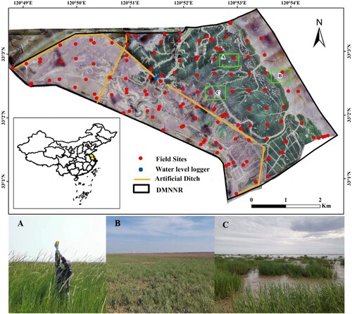
The Dafeng Milu National Nature Reserve (DMNNR), situated at coordinates 32° 56′N-33° 36′N, 120° 42′E-120° 51′E, is located in Dafeng City, within the Yancheng region of Jiangsu Province, China. It is bordered by the Yellow Sea to the east and Dongtai City to the south. The reserve is a typical tidal flat wetland along the Yellow Sea coast. The reserve is located in the transition zone between subtropical and temperate zones and has a marine monsoon climate (Figure 1). The region experiences an annual average temperature ranging from 13.7°C to 14.5°C, and the annual average precipitation varies between 980 and 1100 mm. Most rainfall is concentrated in June and September. The reserve’s fundamental water system is composed of natural tidal creeks and artificial ditches. The third core area of the DMNNR serves as the wild release area for Elaphures davidianus, a deer species native to China and the last extant member of its genus. The main vegetation in the area includes S. alterniflora, Suaeda salsa (L.) Pall, and Aeluropus littoralis var. sinensis of which S. alterniflora accounts for approximately 60% of the total area and is the absolute dominant species in the area (Yan et al. 2021; Yan, Li, Xie et al. 2022).

Figure 1. The location of the Dafeng Milu National Nature Reserve in Jiangsu Province. The background image is a natural true color drone photo taken on August 13, 2020. The unmanned aerial vehicle (UAV) provides a view of the field sample locations, showcasing the varying canopy heights and aboveground biomasses of S. alterniflora. The corresponding field photos, labeled as A, B, and C, were captured at these three sample locations in August 2020.

2.2. Field sampling and laboratory analysis

Large-scale field vegetation sampling was carried out in August 2020 at a 500 m measurement interval, and a total of 140 sampling points were collected including 106 vegetated sampling points and 34 tidal flats sampling points (Figure 1) (more information about the specific sampling location is presented in Supplement A). At each sampling point, three quadrats, each measuring 1 m × 1 m, were randomly established. These were used to record the quantity, coverage, and aboveground biomass of S. alterniflora. Additionally, we used a meter ruler to measure the height of S. alterniflora vegetation. The aboveground parts of all plants in each quadrat were cut with scissors. The aboveground biomass of S. alterniflora was dried at 80° C for 48 hours, and the dry weight was obtained after reaching a constant weight. Finally, 106 vegetated sampling points (318 vegetation samples) and 140 sampling points (420 soil samples) were collected. Meanwhile, a 100 cm³ ring knife was used to collect surface soil at a depth of 0–20 cm. The collected soil samples were cleared of plant residues, snails, shells, gravels, and other impurities. These samples were then naturally dried in a cool place, ground, and pass them through soil sieve. A solution with a water extraction ratio of 5:1 was used to determine the soil salinity by the mass method. The soil conductivity was determined according to the standard procedure (Jackson 2005), and then the relationship between soil electrical conductivity and soil salinity was established by linear fitting, and the soil conductivity was transformed into soil salinity.

2.3. Digital elevation model and canopy height model data acquisition

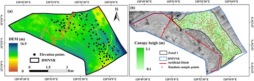
Two UAV flights (UAV platform: Dabai II, wingspan 2.7 m; flight height: 500 m; Dabai Technology Co., Ltd) were chosen for data acquisition due to its capability to generate 40 points/m² point cloud data and further generate digital orthophoto images (40 cm) within the DMNNR. The specific parameters of the UAV are described in the article Yan, Li, Yao et al. (2022). First, we generated the digital surface model (DSM) through the application of multi-view 3D reconstruction technology in the Agisoft Photo Scan 1.2.5 software (Agisoft LLC 2014). In the second step, we employed a GPS-Real Time Kinematic (GPS-RTK) system (a Trimble R8 GNSS; spatial reference: CGCS2000 120E; with a positioning accuracy of 5 mm) to measure 123 ground elevation data points within the S. alterniflora stand as the vegetation was too dense for the UAV point clouds to penetrate the canopy and obtain accurate surface measurements. Finally, we combined the ground elevation points from the dense S. alterniflora vegetation canopy and the bare soil point cloud. Using these combined data, we generated a digital elevation model (DEM) with a spatial resolution of 40 cm using Agisoft PhotoScan. Lastly, we generated the canopy height model (CHM) of S. alterniflora by subtracting the DEM from the DSM (Figure 2b).

Figure 2. Two key components: (a) The digital elevation model (DEM) over the Dafeng Milu National Nature Reserve, and (b) The canopy height model (CHM) of S. alterniflora.

2.4. Methodologies

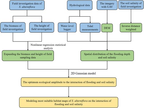
In this study, we developed a method to model the spatial distribution of ecological response of S. alterniflora to the interaction of flooding and soil salinity. This method comprises three parts: (1) expanding the available field sampling; (2) constructing the spatial distribution of flooding depth and soil salinity; (3) generating ecological response curves and developing models to create the most suitable habitat maps for S. alterniflora under the combined influence of inundation and soil salinity. The flow chart of this study is as follows (Figure 3).

Figure 3. The flow chart of modeling the spatial distribution of S. alterniflora ecological response to the interaction of submergence and soil salinity (blue: data acquisition; green: method; Orange: result).

2.4.1. Integrating UAV and field investigation data to determine spatial distribution of S. alterniflora

In this study, we carried out extensive field vegetation sampling at intervals of 500 m, collecting a total of 140 sampling points (equating to 420 samples). Among them, 106 were S. alterniflora communities and 41 were of other types. Although this method is simple and easy to implement, gathering more field data necessitates substantial manpower and resources. Furthermore, the sampling process is complicated by the fact that S. alterniflora is severely affected by tides, which increases the difficulty of sampling. In order to more effectively analyze the impact of water salt interaction on the ecological characteristics of S. alterniflora community, this study integrated UAV and field investigation data to determine spatial distribution of S. alterniflora using nonlinear regression models. This process enabled the acquisition of the spatial distribution of S. alterniflora canopy height and aboveground biomass across the DMNNR. For specifics on the model, refer to Yan, Li, Yao et al. (2022).

However, the field sampling survey found that the stocking of E. davidianus significantly influences S. alterniflora dieback. Many researchers have found that E. davidianus is primarily distributed on the landward side of Dafeng Reserve (Yan et al. 2021; Yan, Li, Xie et al. 2022). To mitigate the effect of E. davidianus on S. alterniflora in this study, 302 samples by the seaward side were randomly selected from the spatial distribution of S. alterniflora plant height and biomass simulated by the model for further study (Figure 2b).

2.4.2. Spatial distribution of the submerged depth and soil salinity

Based on the geomorphological characteristics, Odyssey water level recorders, were strategically placed in the tidal creek (Figure 1). Their purpose is to automatically monitor and document the surface tidal water levels. From 17 May 2020 to 17 May 2021, tidal level data are recorded every 30 min to describe the annual average tidal water level change. Due to the positioning of the water level sensor, it is unable to record water levels unless there is flooding. This limitation prevents the acquisition of a complete annual water level curve in the study area from the water level recorders. To address this, the gap filling program method was employed. This allowed for the filling of the water level time series using the tidal level of the Dafeng tidal station as a reference. From this, a complete one-year water level time series curve is obtained, resulting in an average one-year lunar daily water level curve (Figure 4a). We also calculated the average of the one-year water level time series as the mean sea level (MSL), and define the elevation of MSL as zero. Finally, combining the MSL elevation and DEM, the absolute elevation of the entire study area was converted into relative elevation and inundation depth (Figure 4b).

Figure 4. (a) The red solid line represents the daily average water level curve of the lunar calendar; (b) Spatial distributions of inundation depth, derived from the one-year water level curve and DEM, and (c) The spatial distribution of soil salinity across the Dafeng Milu National Nature Reserve.

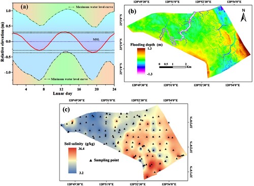
Research has indicated that the accuracy of the spatial distribution of soil salinity across the entire study area, specifically in the 0–20 cm surface soil salinity, is high when using inverse distance weighted (IDW) interpolation (Sheng et al. 2021; Zhao et al. 2019). This method is particularly effective for areas with uniform and densely distributed sampling points (Watson and Philip 1985; Zhao et al. 2019). Consequently, the spatial distribution map of soil salinity in the study area was constructed using IDW, a feature available in the geostatistical toolbox of ArcGIS 10.5 software (Figure 4c).

2.4.3. 3d Gaussian logistic regression model

A 3D surface fitting of the Gaussian model was applied to the S. alterniflora canopy height and environmental gradients, such as flooding and salinity. This process facilitated the determination of the optimal submerged depth and soil salinity ecological range of S. alterniflora under the combined influence of water and salt. The Gaussian model equation is as follows: $\mathrm{z}=z_0+\mathrm{Aexp}[-{\displaystyle \frac{1}{2}(x-x_0{)}^2/w_1^2-{\displaystyle \frac{1}{2}(y-y_0{)}^2/w_2^2]}}$

In this context, z denotes the characteristic index of the plant species, while x and y represent two environmental gradients. The optimum points of environmental gradients x and y are represented by x₀ and y₀, respectively. z₀ and A represent the maximum value of y under the interaction of the two optimal environmental gradients x and y. The tolerances of the vegetation community to environmental gradients x and y are denoted by w₁ and w₂, respectively, which serve as indices describing the ecological range of plant. The range of environmental gradients x is [x₀−w₁, x₀ + w₁], and for y, it is [y₀−w₂, y₀ + w₂] (Yan, Li, Yao et al. 2022; Coudun and Gégout 2006). In this study, 3D Gaussian logistic regression analysis was conducted on the relationship between the physiological characteristics of S. alterniflora and both submergence depth and soil salinity. Origin 2021 software was utilized for curve fitting and data analysis.

2.4.4. Simulation of the spatial distribution of plant height and aboveground biomass of S. alterniflora

In this study, we used the spatial distribution of inundation depth, soil salinity, and the 3D Gaussian model under the combined influence of water-salt to simulate the spatial distribution of S. alterniflora height and biomass across the entire study area. This simulation was performed using the ArcGIS 10.5 spatial analysis tool on the GIS platform.

2.4.5. Model validation of S. alterniflora

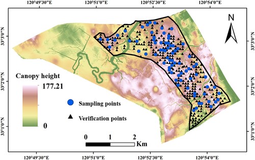
To assess the precision on the spatial simulation of S. alterniflora height and biomass, we primarily verified the accuracy of the model by selecting three statistical indicators: the coefficient of determination (R²), mean absolute percentage error (MAPE), and the ±30% error range. The closer R² is to 1, the higher the degree of fit of the model; the smaller the value of MAPE, the smaller the error between the predicted value and the actual value, and the better the estimation ability of the model. For this study, a dataset of 203 field data points was used for analysis, and field data from 99 field sampling points were used for validation (Figure 5).

Figure 5. Spatial distribution of field verification points for S. alterniflora height and biomass.

3. Results

3.1. Response of S. alterniflora to water-salt interaction

The results of the statistical analysis indicated that the interaction of water and salinity significantly influenced the canopy height and aboveground biomass of S. alterniflora (Table 1). Both relationships displayed the same trend and adhered to the 3D Gaussian logistic regression model. This analysis yielded three-dimensional Gaussian fitting surface regression equations. With a significance level of P < 0.001, the correlation was found to be highly significant (Table 1).

Table 1. The coefficients of the two-dimensional Gaussian regression model corresponding to S. alterniflora and the optimal ecological range of environmental factors.

Physiological Characteristics of S. alterniflora	Coefficient							Ecological Amplitude (u ± t) (P < 0.001)
	Z0	A	X0	Y0	W1	W2	R^2	Flooding depth	Soil salinity
Canopy height	43.12	134.09	0.39	17.83	0.69	8.96	0.73	0.39 ± 0.69 m	17.83 ± 8.96 g/kg
Aboveground biomass	657.36	2088.02	0.38	17.80	0.64	8.33	0.72	0.38 ± 0.64 m	17.80 ± 8.3 g/kg
Intersection of the optimal ecological amplitude								[0, 1.02 m]	[9.47, 26.13 g/kg]

Under the interaction of inundation and soil salinity, the change of S. alterniflora canopy height and aboveground biomass with the increase of flooding depth and soil salinity were consistent with that of single factor (flooding depth or soil salinity), both of which increased first and then decreased. The optimal ecological ranges of S. alterniflora plant height in response to flooding depth and soil salinity were [0, 1.08 m] and [8.87, 26.79 g/kg], respectively, with optimal growth points at 0.39 m and 17.83 g/kg, respectively (Figure 6a). When considering S. alterniflora aboveground biomass, the optimal ecological ranges in response to flooding depth and soil salinity were [0, 1.02 m] and [9.47 g/kg, 26.13 g/kg], respectively, with optimal growth points at 0.38 m and 17.80 g/kg, respectively (Figure 6b). Upon intersecting the optimal ecological ranges based on S. alterniflora plant height and aboveground biomass, the optimal ecological range in response to inundation depth was determined to be [0, 1.02 m] with an optimal mean growth point at 0.38 m. Similarly, the optimal ecological range in response to soil salinity was [9.47 g/kg, 26.13 g/kg] with an optimal mean growth point at 17.80 g/kg. These results suggest that S. alterniflora exhibits optimal growth within these ranges of depth and salinity.

3.2. Modeling the suitable spatial distribution of S. alterniflora response to water-salt interaction

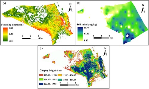
The S. alterniflora canopy height and aboveground biomass initially increased and then decreased with the rise in flooding depth and soil salinity (Figure 6). Based on the ecological amplitude of S. alterniflora, a distribution map was created, highlighting the most suitable habitat for inundation depth, soil salinity, S. alterniflora canopy height, and aboveground biomass. As depicted in Figure 7a, the optimal distribution area for submergence depth, based on S. alterniflora canopy height, is 1665.50 ha, accounting for 67% of the study area. Excluding tidal ditches and relatively high terrain, most areas are conducive to the growth of S. alterniflora, with an optimal submergence depth of 0.39 m. The yellow area in Figure 7a represents the optimal flooding depth for S. alterniflora to achieve maximum plant height. The optimal distribution area of flooding depth, based on S. alterniflora canopy height, was 1857.79 ha, accounting for 74% of the study area. The optimum soil salinity was 17.83 g/kg, and the blue–green area in Figure 7b represents the optimal soil salt distribution area for S. alterniflora to achieve the highest plant height. Upon intersecting the above two distribution areas, the optimal distribution range of S. alterniflora plant height was obtained, covering an area of 1474.88 ha (Figure 7c). The two regions with higher plant height (blue–green: 150.11–164.23 cm and blue: 164.23–177.21 cm) correspond to the optimal submergence depth and soil salinity distribution range (Figure 7).

Figure 6. The height (a) and aboveground biomass (b) of S. alterniflora along the interaction of inundation and soil salinity.

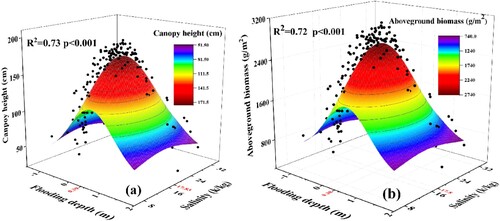
Figure 7. Spatial distribution map of the optimal habitat based on S. alterniflora canopy height for flooding depth(a), soil salinity (b), and canopy height (c).

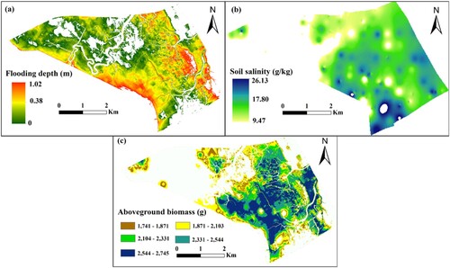
Similar to the optimal spatial distribution of the S. alterniflora canopy height. It can be seen from Figure 8a that the optimal distribution area of flooding depth based on S. alterniflora biomass is 1585.77 ha. Apart from tidal ditches and areas with relatively high terrain, the majority of the region is conducive to the growth of S. alterniflora, which has an optimal submergence depth of 0.38 m. In Figure 8a, the yellow area represents the optimal flooding depth for S. alterniflora to achieve maximum aboveground biomass. The optimal distribution area of soil salinity based on S. alterniflora aboveground biomass was 1650.94 ha, accounting for 74% of the study area (Figure 8b). The optimal soil salinity was determined to be 17.80 g/kg. The blue–green area in Figure 7b represents the optimal soil salt distribution area for S. alterniflora to achieve maximum aboveground biomass. By intersecting the above two distribution areas, the optimal distribution range of S. alterniflora’s aboveground biomass was obtained, covering an area of 1307.99 ha (Figure 8c). The two regions with the highest aboveground biomass (blue–green: 2331-2544 g and blue: 2533–2745 g) correspond to the optimal submergence depth and soil salinity distribution range (Figure 8).

Figure 8. Spatial distribution map of the optimal habitat based on the S. alterniflora biomass for inundation depth(a); soil salinity (b) and aboveground biomass (c).

3.3. Validation of spatial simulation results of S. alterniflora

We compared the measured values of the S. alterniflora canopy height and aboveground biomass with the data estimated by the model. The outcomes of the linear regression analysis are depicted in Figure 9. We compared S. alterniflora height and biomass measured in the field and simulated by the model. The results showed good agreement, indicating that the model can provide reasonable prediction results in the study area. In addition, we computed the performance evaluation criteria for both the S. alterniflora height and biomass. The R² values of plant height and aboveground biomass were 0.70 and 0.68, respectively. The MAPE values of plant height and aboveground biomass were 7.14% and 10.28%, respectively.

Figure 9. Scatter plots depicting the observed and simulated S. alterniflora height (a) and aboveground biomass (b). The blue solid line is Linear regression curve of measured values and simulated value of the S. alterniflora; The red solid line is standard line (y = x); the black dashed line is ± 30% error range.

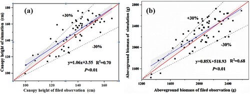
In addition, based on the standard line (red solid line: y = x), ±30% area (black dashed line) was obtained (Figure 9). The findings revealed that 90% of the dispersed points of the observed and simulated values for S. alterniflora plant height and biomass were within the ±30% error range, and the ±30% average error range of plant height and biomass were 96.67–179.52 cm and 1428.47–2652.88 g, respectively. This suggests that the simulation error was less than 30%, thereby validating the accuracy of the simulation outcomes. This level of precision enables us to reliably estimate the S. alterniflora height and biomass in the DMNNR. Thus, the estimation model demonstrates satisfactory performance.

4. Discussion

4.1. Ecological response of S. alterniflora to water-salt interaction

Coastal wetland vegetation is affected by both hydrological and salt factors (Hou 2011; Schile et al. 2017; Snedden, Cretini, and Patton 2015). So far, most researches have focused on the effects of a single factor on the ecological characteristics of S. alterniflora (Li et al. 2018; Luan et al. 2020; Yan, Li, Yao et al. 2022). There are no existing studies on the combined impact of flooding and salt on S. alterniflora in the DMNNR. As of now, our findings are the only data available that demonstrate the interaction of water-salt on S. alterniflora. under the combined influence of water and salt, the optimal ecological range for S. alterniflora’s flooding depth is between 0 m and 1.02 m (Figure 6). Our findings significantly differ from the ecological amplitude of inundation depth (0 m, 0.82 m) of S. alterniflora under the influence of a single factor, as analyzed by Yan, Li, Yao et al. (2022). Our results indicate that the optimal submergence depth ecological range of S. alterniflora under the combined influence of water and salt is larger than that under the influence of a single factor. The optimal ecological range for S. alterniflora’s soil salinity is between 9.47 g/kg and 26.13 g/kg (Figure 6). Similarly, when compared with the salt ecological range of S. alterniflora (13.77 g/kg, 22.57 g/kg) under the influence of single factor soil salt, as analyzed by Yan, Li, Yao et al. (2022), the optimal salt ecological range of S. alterniflora under the interaction of water and salt is larger than that under the influence of single factor soil salt.

If the flooding depth or soil salinity surpasses the tolerance range of S. alterniflora, the interaction between water and salt can reduce its tolerance. As demonstrated by Salter et al. (2007), salinity can restrict the flooding tolerance of Melaleuca ericifolia. This is primarily because high soil salinity can result in plants absorbing insufficient water and mineral nutrients, thereby affecting photosynthesis. Similarly, high flooding depths can induce hypoxia in the roots, inhibiting nutrient absorption and leading to a nutrient deficiency in the aboveground parts of the plant (Carrion 2016; Li et al. 2018). Conversely, low flooding depths can severely impact the growth metabolism of S. alterniflora, causing a significant reduction in photosynthesis and hindering the growth and biomass accumulation of S. alterniflora (Call et al. 2017; Snedden, Cretini, and Patton 2015). When flooding or salinity is within the tolerance range of S. alterniflora, the interaction between water and salt can enhance its tolerance. However, there is currently no relevant research explaining why optimal salinity increases flooding tolerance. In the future, we will conduct in-depth research on this part of the content.

4.2. Modeling the suitable spatial distribution of S. alterniflora response to water-salt interaction

Currently, the emphasis has shifted away from the spatial distribution of wetland vegetation on a small scale. Instead, the focus is now on a larger spatiotemporal scale, where the simulation and predicting of the dynamic interplay between wetland vegetation and ecological hydrological driving mechanisms have become a critical area of study in international wetland ecological hydrological research (Hebb et al. 2013; Zheng et al. 2015). The model we established, based on the diffusion mechanism of S. alterniflora, can predict its spatial distribution pattern. Numerous studies have simulated the spatial distribution of S. alterniflora using remote sensing, GIS technology, and cellular automata Markov models (Yan, Li, Xie et al. 2022; Qin, Yan, and Cai 2020). When landscape and ecological processes undergo change and involve many complex influencing factors, composite models demonstrate strong explanatory power and significant advantages. Currently, many studies have employed the Maximum Entropy (MaxEnt) model and ArcGIS to predict the suitable growth areas of S. alterniflora, considering large-scale climate suitability and environmental variables (Liu 2018; Liu et al. 2019; Sun et al. 2023). However, these models are essentially empirical and do not incorporate inherent driving factors such as hydrology and soil that influence the expansion of S. alterniflora. As a result, the simulation outcomes only represent the distribution range of S. alterniflora, and do not accurately simulate the distribution of plant height and biomass.

The study of how coastal wetland plants respond to the interaction between water and salt in their natural environment is poised to become a significant focus in future wetland ecological research (Ge et al. 2015; He et al. 2007). In our study, Optimal spatial distribution of plant height and biomass of S. alterniflora under water-salt interaction was simulated using a three-dimensional Gaussian model across a larger landscape. As of now, our study provides the only dataset that presents a spatial distribution map of the S. alterniflora response to the interaction between water and salt. In this research, we compared the model results of the S. alterniflora plant height with the spatial distribution of the S. alterniflora plant height obtained by an UAV (Figure 2b). There were some differences in the spatial distribution area of plant height, which was mainly concentrated in the southwest region of the study area. The model simulation results show that the S. alterniflora canopy height is relatively high, whereas the S. alterniflora canopy height obtained by UAV is relatively low. Indeed, this study primarily focuses on the impact of the interaction between water and salt on the spatial distribution of S. alterniflora under natural conditions. It does not take into account the effects of artificial ditches and grazing by E. davidianus on S. alterniflora (Jia et al. 2022; Yan et al. 2021). As a result, the spatial distribution of S. alterniflora’s plant height observed in this study aligns with the distribution obtained via UAV surveillance.

4.3. Uncertainty and future perspectives of modeling the spatial distribution of S. alterniflora with respect to the interaction of flooding and soil salinity

To enhance the modeling of the suitable spatial distribution of S. alterniflora in response to water-salt interaction, we have incorporated field sampling data and utilized a 3D Gaussian logistic regression model. This approach allows us to simulate the distribution of S. alterniflora in a larger landscape. However, UAV has two errors in modeling the spatial distribution of flooding depth and soil salinity, compared with airborne LiDAR, which is more accurate and has enormous potential for monitoring the canopy height and underlying surface elevation of S. alterniflora in the future (Iersel et al. 2018; Zhu et al. 2019). Indeed, a second point to consider is the discrepancy in spatial resolution between the spatial distribution maps of soil salinity (Figure 4b) and flooding depth (Figure 4a) in the study area (Qi et al. 2021).

S. alterniflora is predominantly found in the middle and low intertidal zones, with tidal flooding being a crucial determinant of the S. alterniflora community’s characteristics (Luan et al. 2020; Moffett and Gorelick 2016). The rise in sea level directly extends the duration of tidal inundation and increases both the frequency and depth of inundation, which will likely impact the growth of S. alterniflora in the near future. Numerous studies have indicated that an increase in daily flooding time leads to the replacement of Phragmites australis, located in the high tidal flat, by S. alterniflora and Scirpus mariqueter. The original S. alterniflora and S. mariqueter communities subsequently degrade into mudflats or become submerged (Li 2015; Li 2021). Gong et al. (2019) discovered that under rising sea levels, the flooding time of various coastal wetland ecosystems surpasses their optimal ecological amplitude, resulting in the degradation of wetlands into mudflats. Based on our findings, we determined the optimal tidal inundation and soil salinity ecological range for the S. alterniflora community. Therefore, with the optimal submergence ecological range of S. alterniflora in this study, different flooding depths (beyond the optimal tolerance range) were used for different plant height of S. alterniflora, which provides an effective means for informing the practice of hydrologic control on S. alterniflora (Gong et al. 2019; Stralberg et al. 2011; Xie and Han 2018). In addition to the tidal inundation and soil salinity discussed in this study, the influence of other factors such as temperature and soil nutrients on S. alterniflora should be thoroughly considered (Yan, Li, Yao et al. 2022). Future research should aim to comprehensively explore various environmental factors affecting S. alterniflora to improve the accuracy of simulation results.

5. Conclusions

In this research, we integrate several in situ sampling data and UAV point cloud data to quantitatively evaluate the ecological response of S. alterniflora to the interaction of inundation and soil salinity. We employed a 3D Gaussian model to simulate the most suitable habitat maps of S. alterniflora species across an expansive landscape. We determined the optimal ecological amplitude for S. alterniflora species under the combined influence of inundation and soil salinity. Our analyses further highlighted that the interaction between flooding and soil salinity has a more substantial impact on S. alterniflora than a single factor. The optimal habitat distribution areas for S. alterniflora canopy height and aboveground biomass are 1474.88 ha and 1307.99 ha, respectively. Areas with high S. alterniflora canopy height and aboveground biomass align with the optimal distribution of inundation depth and soil salinity. As of now, our study provides the only dataset that presents a spatial distribution map of S. alterniflora’s response to the interaction between water and salt at the landscape scale. The findings of this study will offer a scientific foundation for the ecological control and prediction of the distribution of S. alterniflora in light of future sea level rise.

Acknowledgements

The study of this paper was supported by the National Natural Science Foundation of China (project no. 41871097, 41471078); PhD Research Startup Foundation of Henan University of Science and Technology (grant number 13480078); Natural Science Foundation of Henan Province (project no. 232300420170); Science and Technology Research Projects of Henan Province (project no. 242102111098).

Disclosure statement

No potential conflict of interest was reported by the author(s).

Data availability

Data will be made available on request.

Additional information

Funding

The study of this paper was supported by the National Natural Science Foundation of China [project no. 41871097, 41471078]; PhD Research Startup Foundation of Henan University of Science and Technology [grant number 13480078]; Natural Science Foundation of Henan Province [project no. 232300420170]; Science and Technology Research Projects of Henan Province [project no. 242102111098].

References

- Agisoft LLC. 2014. “Agisoft PhotoScan User Manual: Professional Edition”, Version 1.1. Accessed 22 August 2021. https://docplayer.net/14282795-Agisoft-photoscan-user-manual-professional-edition-version-1-1.html.
- Burns, T. N. D. 2015. Spartina Alterniflora Responses to Flooding in Two Salt Marshes on the Eastern Shore of Virginia. Charlottesville: University of Virginia. Commonwealth of Virginia, The United States of America.
- Call, B. C., P. Belmont, J. C. Schmidt, and P. R. Wilcock. 2017. “Changes in Floodplain Inundation Under Nonstationary Hydrology for an Adjustable, Alluvial River Channel.” Water Resources Research 53:3811–3834. https://doi.org/10.1002/2016WR020277.
- Carrion, S. A. 2016. Determining Factors That Influence Smooth Cordgrass (Spartina Alterniflora Loisel) Transplant Success in Community-Based Living Shoreline Projects. Orlando, FL: University of Central Florida, The United States of America.
- Coudun, C., and J. C. Gégout. 2006. “The Derivation of Species Response Curves with Gaussian Logistic Regression is Sensitive to Sampling Intensity and Curve Characteristics.” Ecological Modelling 199:164–175. https://doi.org/10.1016/j.ecolmodel.2006.05.024.
- Cui, L. J., W. Li, Z. G. Dou, M. Y. Zhang, G. F. Wu, Z. W. Hu, Y. Gao, J. Li, and Y. R. Lei. 2022. “Changes and Driving Forces of the Tidal Flat Wetlands in Coastal China During the Past 30 Years.” Acta Ecologica Sinica 42:7297–7307. https://doi.org/10.5846/stxb202203080551.
- Ge, Z. M., H. B. Cao, L. F. Cui, B. Zhao, and L. Q. Zhang. 2015. “Future Vegetation Patterns and Primary Production in the Coastal Wetlands of East China Under sea Level Rise, Sediment Reduction, and Saltwater Intrusion.” Journal of Geophysical Research: Biogeosciences 120:1923–1940. https://doi.org/10.1002/2015JG003014.
- Gong, H. B., H. Y. Liu, F. S. Jiao, Z. S. Lin, and X. J. Xu. 2019. “Pure, Shared, and Coupling Effects of Climate Change and Sea Level Rise on the Future Distribution of Spartina alterniflora Along the Chinese Coast.” Ecology and Evolution 9:5380–5391. https://doi.org/10.1002/ece3.5129.
- Guisan, A., T. C. Edwards, and T. Hastie. 2002. “Generalized Linear and Generalized Additive Models in Studies of Species Distributions: Setting the Scene.” Ecological Modelling 157:89–100. https://doi.org/10.1016/S0304-3800(02)00204-1.
- Han, G. X., F. M. Wang, J. Ma, L. L. Xiao, X. J. Chu, and M. L. Zhao. 2022. “Blue Carbon Sink Function, Formation Mechanism and Sequestration Potential of Coastal Salt Marshes.” Chinese Journal of Plant Ecology 46:373–382. https://doi.org/10.17521/cjpe.2021.0264.
- He, Q., B. S. Cui, X. S. Zhao, H. L. Fu, X. Xiong, and G. H. Feng. 2007. “Vegetation Distribution Patterns to Gradients of Water Depth and Soil Salinity in Wetlands of Yellow River Delta, China.” Science of Wetlands 5:208–214. https://doi.org/10.13248/j.cnki.wetlandsci.2007.03.001.
- Hebb, A. J., L. D. Mortsch, P. J. Deadman, and A. R. Cabrera. 2013. “Modeling Wetland Vegetation Community Response to Water-Level Change at Long Point, Ontario.” Journal of Great Lakes Research 39:191–200. https://doi.org/10.1016/j.jglr.2013.02.001.
- Hou, D. 2011. Study on Succession and Ecological Thresholds of Natural Ecosystem in Yellow River Delta. People’s Republic of China: Shandong Agricultural University. Tai’an, Shandong Province.
- Iersel, W., M. Straatsma, E. Addink, and H. Middelkoop. 2018. “Monitoring Height and Greenness of non-Woody Floodplain Vegetation with UAV Time Series.” ISPRS Journal of Photogrammetry and Remote Sensing 141:112–123. https://doi.org/10.1016/j.isprsjprs.2018.04.011.
- Jackson, M. L. 2005. “Soil Chemical Analysis: Advanced Course.” UW-Madison Libraries Parallel Press, Madison, Wisconsin, The United States of America.
- Jia, Y. Y., S. B. Xie, H. P. Yuan, and L. L. Lu. 2022. “Effects of Wild elk Activities on Some Ecological Indexes of Spartina alterniflora.” Journal of Anhui Agricultural Sciences 50:63–65. https://doi.org/10.3969/j.issn.0517-6611.2022.15.017.
- Kirwan, M. L., R. R. Chrisian, L. K. Blum, and M. M. Brinson. 2012. “On the Relationship Between Sea Level and Spartina alterniflora Production.” Ecosystems 15:140–147. https://doi.org/10.1007/s10021-011-9498-7.
- Li, S. S. 2015. Vulnerability Assessment of the Coastal Mangrove Ecosystems in Guangxi, China to Sea-Level Rise. Shanghai: East China Normal University.
- Li, J. 2021. Study on Population Dynamics and Diffusion Model of Invasive Plant Spartina alterniflora. People’s Republic of China: North China University of Science and Technology. Tangshan, Hebei Province.
- Li, W., L. Yuan, Z. Y. Zhang, H. Li, X. J. Zhu, J. L. Pan, and Y. H. Chen. 2018. “Responses of Scirpus mariqueter and Spartina alterniflora to Simulated Salt Stress and Salttolerance Thresholds.” Chinese Journal of Ecology 37:2596–2602. https://doi.org/10.13292/j.1000-4890.201809.023.
- Liu, M. Y. 2018. “Remote Sensing Analysis of Spartina alterniflora in the Coastal Areas of China during 1990 to 2015.” Northeast Institute of Geography and Agroecology, Chinese Academy of Sciences. Changchun, Jilin Province, People’s Republic of China.
- Liu, M. Y., D. H. Mao, Z. M. Wang, L. Li, W. D. Man, M. M. Jia, C. Y. Ren, and Y. Z. Zhang. 2018. “Rapid Invasion of Spartina alterniflora in the Coastal Zone of Mainland China: New Observations from Landsat OLI Images.” Remote Sensing 10:1933. https://doi.org/10.3390/rs10121933.
- Liu, H. Y., X. Z. Qi, H. B. Gong, L. H. Li, M. Y. Zhang, Y. F. Li, and Z. S. Lin. 2019. “Combined Effects of Global Climate Suitability and Regional Environmental Variables on the Distribution of an Invasive Marsh Species Spartina alterniflora.” Estuaries and Coasts 42:99–111. https://doi.org/10.1007/s12237-018-0447-y.
- Lou, Y. J., C. Y. Gao, Y. W. Pan, Z. S. Xue, Y. Liu, Z. H. Tang, M. Jiang, X. G. Lu, and H. Rydin. 2018. “Niche Modelling of Marsh Plants Based on Occurrence and Abundance Data.” Science of The Total Environment 616:198–207. https://doi.org/10.1016/j.scitotenv.2017.10.300.
- Luan, Z. Q., D. D. Yan, Y. Y. Xue, D. Shi, D. D. Xu, B. Liu, L. B. Wang, and Y. T. An. 2020. “Research Progress on the Ecohydrological Mechanisms of Spartina alterniflora Invasion in Coastal Wetlands.” Journal of Agricultural Resources and Environment 37:469–476. https://doi.org/10.13254/j.jare.2019.0124.
- Moffett, K. B., and S. M. Gorelick. 2016. “Relating Salt Marsh Pore Water Geochemistry Patterns to Vegetation Zones and Hydrologic Influences.” Water Resources Research 52:1729–1745. https://doi.org/10.1002/2015WR017406.
- Moreira, L. L., R. A. Tavella, A. S. Bonifácio, R. L. Brum, L. S. Freitas, N. G. R. Moraes, M. L. Fiasconaro, et al. 2024. “Bioaccumulation of Metals in Spartina alterniflora Salt Marshes in the Estuary of the World’s Largest Choked Lagoon.” Environmental Science and Pollution Research 31:26880–26894. https://doi.org/10.1007/s11356-024-32810-3.
- Oksanen, J., and P. R. Minchin. 2002. “Continuum Theory Revisited: What Shape are Species Responses Along Ecological Gradients?” Ecological Modelling 157:119–129. https://doi.org/10.1016/S0304-3800(02)00190-4.
- Parihar, P., S. Singh, R. Singh, V. P. Singh, and S. M. Prasad. 2015. “Effect of Salinity Stress on Plants and its Tolerance Strategies: A Review.” Environmental Science and Pollution Research 22:4056–4075. https://doi.org/10.1007/s11356-014-3739-1.
- Qi, G. H., C. Y. Chang, W. Yang, P. Gao, and G. X. Zhao. 2021. “Soil Salinity Inversion in Coastal Corn Planting Areas by the Satellite-UAV-Ground Integration Approach.” Remote Sensing 13:3100. https://doi.org/10.3390/rs13163100.
- Qin, Y. L., Q. S. Yan, and J. H. Cai. 2020. “Evolution and Dynamic Simulation of Landscape Pattern in the South Part of Poyang Lake Wetland.” Journal of Yangtze River Scientific Research Institute 37:171–178. https://doi.org/10.11988/ckyyb.20190252.
- Salter, J., K. Morris, P. Bailey, and P. I. Boon. 2007. “Interactive Effects of Salinity and Water Depth on the Growth of Melaleuca ericifolia Sm.” Aquatic Botany 86:213–222. https://doi.org/10.1016/j.aquabot.2006.10.002.
- Schile, L. M., J. C. Callaway, K. N. Suding, and N. M. Kelly. 2017. “Can Community Structure Track sea-Level Rise? Stress and Competitive Controls in Tidal Wetlands.” Ecology and Evolution 7:1276–1285. https://doi.org/10.1002/ece3.2758.
- Sheng, J., P. Yu, H. N. Zhang, and Z. L. Wang. 2021. “Spatial Variability of Soil Cd Content Based on IDW and RBF in Fujiang River, Mianyang, China.” Journal of Soils and Sediments 21:419–429. https://doi.org/10.1007/s11368-020-02758-1.
- Snedden, G. A., K. Cretini, and B. Patton. 2015. “Inundation and Salinity Impacts to Above- and Belowground Productivity in Spartina Patens and Spartina alterniflora in the Mississippi River Deltaic Plain: Implications for Using River Diversions as Restoration Tools.” Ecological Engineering 81:133–139. https://doi.org/10.1016/j.ecoleng.2015.04.035.
- Stralberg, D., M. Brennan, J. C. Callaway, J. K. Wood, L. M. Schile, D. Jongsomjit, M. Kelly, V. T. Parker, and S. Crooks. 2011. “Evaluating Tidal Marsh Sustainability in the Face of Sea-Level Rise: A Hybrid Modeling Approach Applied to San Francisco Bay.” PLoS One 6:e27388. https://doi.org/10.1371/journal.pone.0027388.
- Sun, S., H. C. Xian, Z. Y. Hu, X. X. Sun, and F. Zhang. 2023. “Physical Processes Determining the Distribution Patterns of Nemopilema nomurai in the East China Sea.” Journal of Oceanology and Limnology 41:2160–2165. https://doi.org/10.1007/s00343-023-2370-8.
- Tang, L., Y. Gao, B. Li, Q. Wang, C. H. Wang, and B. Zhao. 2014. “Spartina alterniflora with High Tolerance to Salt Stress Changes Vegetation Pattern by Outcompeting Native Species.” Ecosphere (Washington, D C) 5:1. https://doi.org/10.1890/ES14-00166.1.
- Wang, C., Q. Wang, D. Meire, W. D. Ma, C. Q. Wu, Z. Meng, J. Van de Koppel, et al. 2016. “Biogeomorphic Feedback Between Plant Growth and Flooding Causes Alternative Stable States in an Experimental Floodplain.” Advances in Water Resources 93:223–235. https://doi.org/10.1016/j.advwatres.2015.07.003.
- Watson, D. F., and G. M. Philip. 1985. “A Refinement of Inverse Distance Weighted Interpolation.” Geoprocessing 2:315–327.
- Xie, B. H., and G. X. Han. 2018. “Control of Invasive Spartina alterniflora: A Review.” Chinese Journal of Applied Ecology 29:3464–3476. https://doi.org/10.13287/j.1001-9332.201810.006.
- Xue, Y. Y., D. D. Yan, L. P. Qi, J. T. Li, and Z. Q. Luan. 2022. “Ecological Response of Spartina alterniflora Towards Moisture and Salinity Gradients in Dafeng Elk National Nature Reserve Jiangsu Province.” Acta Scientiae Circumstantiae 42:28–35. https://doi.org/10.13671/j.hjkxxb.2021.0489.
- Yan, D. D., J. T. Li, S. Y. Xie, Y. Liu, Y. F. Sheng, and Z. Q. Luan. 2022. “Examining the Expansion of Spartina alterniflora in Coastal Wetlands Using an MCE-CA-Markov Model.” Frontiers in Marine Science 9:964172. https://doi.org/10.3389/fmars.2022.964172.
- Yan, D. D., J. T. Li, X. Y. Yao, and Z. Q. Luan. 2021. “ Quantifying the Long-Term Expansion and Dieback of Spartina alterniflora Using Google Earth Engine and Object-Based Hierarchical Random Forest Classification.” IEEE Journal of Selected Topics in Applied Earth Observations and Remote Sensing 14:9781–9793. https://doi.org/10.1109/JSTARS.2021.3114116.
- Yan, D. D., J. T. Li, X. Y. Yao, and Z. Q. Luan. 2022. “Integrating UAV Data for Assessing the Ecological Response of Spartina alterniflora Towards Inundation and Salinity Gradients in Coastal Wetland.” Science of The Total Environment 814:152631. https://doi.org/10.1016/j.scitotenv.2021.152631.
- Yan, D. D., Z. Q. Luan, D. D. Xu, Y. Y. Xue, and D. Shi. 2020. “Modeling the Spatial Distribution of Three Typical Dominant Wetland Vegetation Species’ Response to the Hydrological Gradient in a Ramsar Wetland, Honghe National Nature Reserve, Northeast China.” Water 12:2041. https://doi.org/10.3390/w12072041.
- Zhang, X., X. M. Xiao, X. X. Wang, X. Xu, B. Q. Chen, J. Wang, J. Ma, Z. Bin, and B. Li. 2020. “Quantifying Expansion and Removal of Spartina alterniflora on Chongming island, China, Using Time Series Landsat Images During 1995-2018.” Remote Sensing of Environment 247:111916. https://doi.org/10.1016/j.rse.2020.111916.
- Zhao, W. J., T. H. Cao, Z. L. Li, and J. Sheng. 2019. “Comparison of IDW, Cokriging and ARMA for Predicting Spatiotemporal Variability of Soil Salinity in a Gravel-Sand Mulched Jujube Orchard.” Environmental Monitoring and Assessment 191:376. https://doi.org/10.1007/s10661-019-7499-8.
- Zheng, Z. S., B. Tian, L. W. Zhang, and G. L. Zou. 2015. “Simulating the Range Expansion of Spartina alterniflora in Ecological Engineering Through Constrained Cellular Automata Model and GIS.” Mathematical Problems in Engineering 2015:1. https://doi.org/10.1155/2015/875817.
- Zhu, X. D., L. X. Meng, Y. H. Zhang, Q. H. Weng, and J. Morris. 2019. “Tidal and Meteorological Influences on the Growth of Invasive Spartina alterniflora: Evidence from UAV Remote Sensing.” Remote Sensing 11:1208. https://doi.org/10.3390/rs11101208.