Green space coverage versus air pollution: a cloud-based remote sensing data analysis in Sichuan, Western China

ABSTRACT

Air pollution is the greatest health risk to human health, as acknowledged in several Sustainable Development Goals (SDG), such as SDG-1, SDG-3, SDG-7, and SDG-11. Despite global comprehension of the positive effect of Green Space Coverage (GSC) on mitigating air pollution, investigating the impact of different GSC types has received little attention. Here, we utilized multiple air pollution data and a cloud-computing platform to examine the role of different GSC types in mitigating NO₂ and PM2.5 pollutants across 2019 and 2022 in Sichuan Province, China. We classified GSC areas into tall GSC and short GSC classes, taking into account the recognized importance of vegetation height in prior studies. Our analysis revealed that tall GSCs exhibit lower pollutant levels across all areas studied, indicating a potential correlation between GSC height and pollution mitigation efficacy. Furthermore, in high human activity areas, while tall GSC emerged as effective sinks for PM 2.5 compared to short GSC (25% and 20% lower average annual in 2019 and 2022, respectively), their performance in reducing NO₂ pollutant levels was relatively limited (9% and 4% lower average annual in 2019 and 2022, respectively). These findings can contribute to urban planning and environmental management.

KEYWORDS:

• Air pollution; green coverage; sustainable development; remote sensing
• Sichuan
• China

1. Introduction

Air pollution is predominantly an unwanted outcome of urbanization, industrialization, and rapid economic expansion (Rentschler and Leonova 2023; Soleimanpour, Alizadeh, and Sabetghadam 2023). This form of pollution poses the greatest environmental health threat to humans worldwide, resulting in nearly nine million premature deaths annually, accounting for one in six deaths globally (Fuller et al. 2022). Furthermore, it influences productivity (Rentschler and Leonova 2023), worsens inequality (Peeples 2020), diminishes cognitive abilities (La Nauze and Severnini 2021), and amplifies the impact of global warming (Kinney 2018). Given the significant influence of air pollution on human welfare, the United Nations (UN) has incorporated it into formulating Sustainable Development Goals (SDGs). Air pollution has direct correlations with SDG-1, SDG-3, SDG-7, and SDG-11, as well as indirect pathways to support other SDGs, such as SDG-12 (Zhu et al. 2022). For example, providing clean air is essential in supporting SDG-11, which seeks to make communities and cities inclusive, safe, resilient, and sustainable. Expanding Green Space Coverage (GSC) has been proposed as a solution to enhance air quality. However, examining the impact of different GSC types on air pollution mitigation, particularly over large-scale areas, has not received much attention. As a result, understanding the impact of various GSC types on air pollution is critical for promoting the SDGs.

Sichuan Province, a rapidly developing region in China, faces air pollution issues of varying degrees in different cities and at different times (Fang et al. 2021). Sichuan is among the most polluted provinces in China due to its intricate geography and adverse weather conditions (Hu and Wang 2021; Liu et al. 2018). In 2015, with seven days of severe pollution, over 80 percent of cities in the Sichuan province failed to meet the national air quality standards (Zhang et al. 2019). Following an official announcement by Chinese President Xi in 2014, acknowledging the direct impact of air quality on the happiness of the Chinese people, significant endeavors have been undertaken to enhance air quality in both China and Sichuan. For example, in 2018, the Ministry of Ecology and Environment of China released a three-year strategy named ‘Battle for Blue Sky’ to improve air quality. As a result, the expansion of GSC has been implemented in Sichuan, in particular Chengdu city, the capital of Sichuan province (Huang, Fan, and Shen 2019; Zhong et al. 2020). Furthermore, several studies have focused on monitoring air pollution over Sichuan province (Fang et al. 2021; Guo et al. 2022; Hu and Wang 2021; Liu et al. 2018; Ning et al. 2018). Prior studies primarily focused on examining the spatial–temporal distribution of air pollution in Sichuan province. Still, there is a lack of well-documented research on the impact of GSCs on air quality in this region, given its complex terrain and climatic conditions.

It is widely accepted that GSC has reductive impacts on air pollutants through the absorption of pollutants, filtration of particulate matter, production of oxygen, and functioning as windbreaks to disperse pollutants (Lee, Tran, and Yu 2023; Selmi et al. 2016; Yuan, Shin, and Managi 2018). There is no universally recognized definition for ‘green space’, but it is commonly interpreted as outdoor and on-land plants and vegetation (Taylor and Hochuli 2017). Researchers across various disciplines have examined the relationship between GSC and air pollution. For example, Diener and Mudu (2021) employed a systematic review approach to examine a large number of papers. Their thorough examination demonstrated that GSC has significant, diverse, and multi-faceted impacts on reducing air pollution levels, which vary according to the scale, context, and characteristics of the vegetation. In another study, Yuan, Shin, and Managi (2018) examined the influence of air pollution and GSC on the level of life satisfaction in China. Their findings demonstrated a strong and inverse correlation between air pollution and GSC. Furthermore, Zhou et al. 2021 studied the status of air pollutants in 341 cities in China during COVID-19. The researchers employed the Normalized Difference Vegetation Index (NDVI) as an index for GSC mapping. They concluded that there is an inverse relationship between GSC and local pollutant concentration, meaning that higher GSC corresponds to lower pollutant levels.

Prior research undoubtedly provides valuable information on how GSC affects air pollution, but examining the impact of different GSC types on air pollution mitigation, particularly over large-scale areas, has not received much attention. There are multiple criteria, such as vegetation types, leaf area density, canopy cover, and vegetation height, based on which GSC can be classified. While vegetation types (e.g. forest, shrubland, and grasslands) has been commonly used for GSC type classification, vegetation height has been introduced as an important criterion in vegetation's air filtration and purification capabilities (Barwise and Kumar 2020; Taleghani et al. 2020). Tall vegetation, such as trees and large shrubs, typically possesses greater surface area and volume, offering larger coverage and potential for air pollutant absorption. In contrast, short vegetation, including grasses and croplands, may have distinct air purification mechanisms due to their smaller size and form. Therefore, the current study employs vegetation height as a criterion for defining GSC areas to investigate how vegetation height influences air pollution on a larger scale.

Remote Sensing (RS) technology provides a reliable method for constantly tracking air pollution changes at different spatial and temporal ranges (Ghasempour et al. 2021). The use of satellites to monitor air pollution dates back to the 1970s with the utilization of the GOES, Landsat, and AVHRR. Among the pool of satellite data, the recent TROPOspheric Monitoring Instrument (TROPOMI) onboard Sentinel-5P has gained popularity in air pollution monitoring studies due to the reasonable accuracy of this sensor compared to ground observations (Shami et al. 2022). For example, Ialongo et al. 2020 reported a correlation of nearly 0.70 between TROPISM-derived and ground-based air pollution observations. However, TROPOMI has limited application in estimating Particulate Matter (PM) since it is designed to monitor various atmospheric trace gases and aerosols, such as sulfur dioxide (SO2) and nitrogen dioxide (NO2). The commonly used method for estimating PM from satellite data is to determine a relationship between PM concentration and the Aerosol Optical Depth (AOD) determined by the satellite (Yang, Yuan, and Li 2022). To this end, the most commonly used AOD products derive from the Moderate Resolution Imaging Spectroradiometer (MODIS), which has demonstrated acceptable performance for PM estimation (Imani 2021).

Big RS data analysis is required when studying a large-scale region is the objective (Guo et al., 2023). The arrival of cloud computing platforms, such as Google Earth Engine (GEE), allows us to interpret and process large volumes of data (Gorelick et al. 2017). The GEE platform, which hosts a vast amount of geospatial data, enables us to easily visualize and analyze large RS data without downloading the raw data (Bian et al. 2020; Naboureh et al. 2023). Given the aforementioned advantages, many researchers have studied air pollution monitoring using RS data on the GEE platform (Ayyamperumal et al. 2024; Ghasempour, Sekertekin, and Kutoglu 2021; Rabiei-Dastjerdi, Mohammadi, and Saber 2022; Shami et al. 2022; Singh et al. 2021; Wang, Chu, et al. 2022; Wang, Guo, et al. 2022; Wu et al. 2023; Zhang et al. 2020). Most prior researchers treated uniformly urbanized and industrialized areas with High Human Activities (HHA) and other regions with Low Human Activities (LHA) areas. However, it is critical to recognize that the amount and spreading mechanism of air pollution vary across HHA and LHA regions (Phan and Fukui 2024). As a result, this study first investigated how air pollution varies in HHA and LHA zones before examining the effects of different kinds of GSC in these areas.

Given the aforementioned issues, this study utilized air pollution data (satellite and ground truth) to examine the impact of various GSC on two crucial air pollution indicators, namely NO₂ and PM2.5, over Sichuan province. The motivation behind selecting these pollutants is that NO₂ and PM2.5 are the primary components of haze pollution in China (Liu et al. 2018). To mitigate the impact of COVID restrictions on our analysis, we focused exclusively on the years 2019 (before the COVID outbreak) and 2022 (after the COVID outbreak). Some contributions of the present research are as follows:

1.	Combining multi-sensor remote sensing data, ground-based weather station data, and a cloud computing platform to monitor air pollution over a vast region.
2.	Monitor two key air pollution parameters, namely NO2 and PM2.5, in 2019 and 2022 over Sichuan province.
3.	Investigate the disparity in air pollution between the HHA and LHA regions.
4.	Examine the impact of different GSC types on air pollution and how they contribute to air pollution mitigation in HHA and LHA regions.

2. Study area and data

2.1. Study area

Sichuan Province, an evergreen region, is located in southwestern China. This Province spans over 485,000 square kilometers and has a population of roughly 83 million residents. The elevation in this Province varies significantly from west to east, spanning a range of over 7000 to 100 m. High mountains dominate most of the territory in the southern and western areas, while flat plains dominate the eastern section. The unique topography of Sichuan Province blocks the airflow inside the Sichuan basin (eastern side of the Province), resulting in a pronounced heat island effect in the majority of cities in the Province, notably Chengdu, under a subtropical monsoon humid climate.

2.2. Data collection

This study used a combination of ground-based and satellite-based datasets (Table 1): (a) Landsat-8 surface reflectance data for generating the GSC map; (b) TROMPI instrument on board the Sentinel-5P satellite for mapping NO₂; (c) MODIS AOD product for mapping PM 2.5; and (d) in-situ pollutants’ concentration data from weather stations for accuracy assessment.

Table 1. List of four different datasets used in this research.

Data	Use in this study	Data source
Landsat-8	GSC	https://developers.google.com/earthengine/datasets/
Sentinel-5p	NO2	GEE ID = COPERNICUS/S5P/OFFL/L3_NO2
MODIS	PM 2.5	https://weijing-rs.github.io/product.html
Weather station	NO2 and PM2.5	http://www.cnemc.cn/

3. Methods

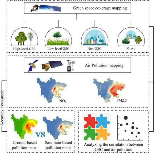
This study investigates the impact of different GSCs on air pollution at the provincial and city levels. Figure 2 illustrates the four primary stages of this study, including GSC mapping, air pollution mapping, accuracy assessment, and the analysis of the correlation between GSC and air pollution. Most of the procedure was performed within the GEE platform, which enabled us to derive pixel-wise analysis without downloading raw data. Given that the amount and spreading mechanism of air pollution vary across HHA and LHA regions (Phan and Fukui 2024), we used the publicly available world population and global artificial impervious area (Gong et al. 2020) developed by scientists from Tsinghua University as well as local experts, to define HHA and LHA zones (Figure 1(a)).

Figure 1. (a) Location of Sichuan Province in China. (b) Map of High Human Activity (HHA) and Low Human Activity (LHA) zones used in this study, along with the boundaries of Sichuan cities. (c) The elevation map of Sichuan and the location of ground-based weather stations used in this study. (d) and (e) An example of air pollution in the Tianfu New Area, Chengdu City in December 2023.

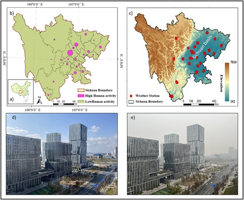
Figure 2. The main workflow of this study.

3.1. GSC mapping

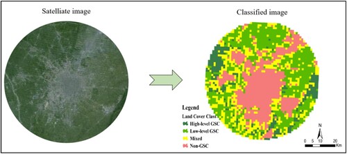
GSCs can potentially to improve air quality; however, the process involved in pollution removal by different GSCs varies depending on their characteristics (Linden et al. 2023). Enhanced by Barwise and Kumar (2020), we have divided the Sichuan province based on the height of the vegetation into tall GSC and short GSC classes. In our research, we also considered the presence of mixed classes. The rationale for this choice is that we have identified multiple pixels that contain a combination of GSC and non-GSC classes. We encountered this issue when we set the spatial resolution of GSC maps to 1100 m to align with the spatial resolution of pollution maps derived from satellite data (see Section 3.2). In general, we consider four classes in our research: tall GSC, short GSC, non-GSC, and mixed classes. Table 2 provides a detailed description of each class.

Table 2. Description of different GSC classes in this study.

Class type	Description
tall GSC	Tall GSC refers to a category of GSC that includes tall vegetation types, such as forests and shrub areas, that exceed a height of 2 meters.
short GSC	The short GSC category includes small GSC types, such as shrubs that are less than 2 meters in height, grasslands, and croplands.
non-GSC	Non-GSC refers to a category that encompasses all areas that are not classified as GSC, including developed areas, bare lands, open water, and snow/ice.
mixed	This class combines characteristics from the three types mentioned above.

We generated one GSC map for both 2019 and 2022 years because the changes in GSC classes between these two years were very small due to the very short (two – year) interval from 2019 to 2022 and the very low possibility of land cover changes occurring due to COVID restrictions. In more detail, we used all available Landsat-8 images for 2019 and 2022. We then applied the FMASK algorithm to each image to eliminate unwanted pixels such as clouds and shadows (Gorelick et al. 2017). Finally, the median function of six spectral bands of Landsat-8 (bands 1-6) was calculated to create the mosaic images for LC classification. Moreover, we calculated two spectral indexes, NDVI and the Enhanced Vegetation Index (EVI), for the classification procedure. We used 1000 reference samples (700 training and 300 validation samples). Finally, this study used a random forest classifier, known for its high performance in various land cover mapping tasks (Ebrahimy et al. 2021; Naboureh et al. 2021), to classify Sichuan into three classes at a 30-m resolution. The generated map showed reasonable accuracy for both the overall and individual classes.

Given the medium resolution of the pollution maps (see Section 3.2), which included several 30-m pixels, we resampled the 30-m resolution GSC map generated by Landsat data into 1100 m pixels to match the air pollution maps using a majority voting method. This entailed calculating the count of each GSC class within each pixel, with the class with the highest majority determining the given value for that pixel's GSC type. In some more detail, a pixel was designated as a class (tall GSC, short GSC, or non-GSC) when it covered over 75% of the pixel; otherwise, it was labeled as a mixed pixel. Finally, two experienced image interpreters used the visual assessment to determine each pixel's final GSC class type. Figure 3 presents an example of our classification result over the HHA zone of Chengdu, the capital of Sichuan province.

Figure 3. An example of the generated GSC map for the HHA of Chengdu City, the capital of Sichuan province.

3.2. Air pollution mapping

As discussed earlier, this research intends to explore the detailed spatial–temporal distribution of two main pollutants, NO₂ and PM 2.5, over Sichuan Province. NO₂ is transmitted into the atmosphere through human activities (e.g. fossil fuel combustion and biomass burning) and natural processes (e.g. microbiological processes in lightning, firing, and soil). PM 2.5 is primarily a result of combustion processes such as vehicle engines, industrial processes, dust storms, and wildfires (Yang, Yuan, and Li 2022; Xu et al., 2023). It has been stated that over 500 million urban residents are at risk of severe PM 2.5 pollution in China (Li and Huang 2020). We chose these two pollutants for this investigation because of their harmful effects on human health in China.

The NO₂ distribution maps for 2019 and 2022 were derived from the TROPOMI instrument (between 1st January and 31st December) through the GEE platform. TROMPI measures the solar radiation reflected by the Earth while employing passive RS techniques to reach the target above the atmosphere. This study used the vertical column density at the ground level of offline level 3 NO2 in 0.01 arc degree (∼1100 m) spatial resolution. Notably, we removed pixels with values less than 75% and 50% Quality Assurance (QA) from the NO₂ products. Finally, after applying the temporal and spatial filters, NO₂ products from the region were produced monthly and annually for both the 2019 and 2022 years.

Multiple researchers (Xiao et al., 2015; Wei et al. 2020) have documented strong correlations between ground-based and satellite-retrieved PM values. Therefore, we used 1-km PM 2.5 data provided by Wei et al. 2021, which is freely available (see Table 1) and covers daily, monthly, and yearly intervals between 2000 and 2022. The data set was created by combining the MODIS AOD product with ground station PM2.5 data using the multi-angle implementation of the atmospheric correction algorithm. This data set demonstrates a remarkably high accuracy in measuring PM2.5 concentrations across various spatial and temporal dimensions in China (i.e. the cross-validation coefficient of determination (CV-R2) ranges from 0.86 to 0.90). In this study, we used the monthly and annual products for 2019 and 2022.

3.3. Accuracy assessment

The accuracy assessment task used ground-based NO₂ and PM2.5 data from the China national environmental monitoring center. The provided information from 93 stations in 2019 and 103 stations in 2022 was used for verification (see Figure 4). To this end, we used the Kriging spatial interpolation method to derive seasonal and annual NO₂ and PM2.5 for 2019 and 2022 based on the in-situ data. Kriging uses measured values and their correlation characteristics to estimate unknown values (Longley et al., 1997). After obtaining monthly and annual pollution maps from in-situ data, we compared them against satellite-based air pollution maps using correlation coefficient (R) and Root Mean Square Error (RMSE), Standard Deviation of Error (STD Error), and Bias metrics. (1) $R={\displaystyle \frac{\sum (y_i-{\overline{y}}_i)(x_i-{\overline{x}}_i)}{\sqrt{\sum {(y_i-{\overline{y}}_i)}^2}\sum {(x_i-{\overline{x}}_i)}^2}}$(1) (2) $\mathrm{RMSE}=\sqrt{{\displaystyle \frac{\sum {(x_i-y_i)}^2}{n}}}$(2) (3) $\mathrm{SDT}\mathrm{of}\mathrm{Error}=\sqrt{{\displaystyle \frac{\sum {(y_{\mathrm{Error}}-{\overline{y}}_{\mathrm{Error}})}^2}{n}}}$(3) (4) $\mathrm{Bias}={\displaystyle \frac{\sum (x_i-y_i)}{n}}$(4)

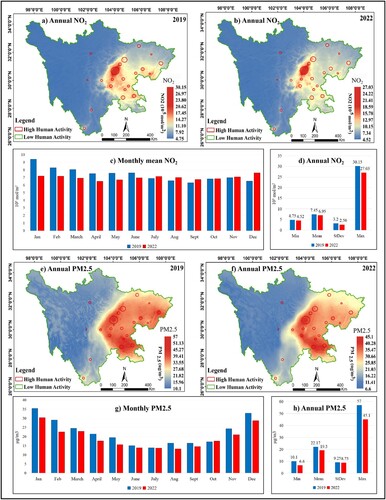
Figure 4. (a) & (b) Satellite-based NO₂ retrieval for 2019 and 2022 over Sichuan Province. (c) Monthly mean value of NO₂ over Sichuan Province. (d) Annual min, max, mean, and StDev values of NO₂ over Sichuan Province. (e) & (f) Satellite-based PM2.5 retrieval for the years 2019 and 2022 over Sichuan Province. (g) Monthly mean value of PM2.5 over Sichuan Province. (h) Annual min, max, mean, and StDev values of PM2.5 over Sichuan Province.

Where y_i, x_i, ${\overline{y}}_i$, and ${\overline{x}}_i$ are the Satellite-derived pollution maps, ground-based pollution maps, and their average values, respectively. $y_{\mathrm{Error}}$ represents the difference between satellite-derived and ground-based pollution maps, and ${\overline{y}}_{\mathrm{Error}}$ refers to the average of differences.

3.4. GSC and air pollution

To examine the impact of various GSC types (discussed in Section 3.1) on air pollution mitigation (discussed in Section 3.2), we employed two separate areas: HHA and LHA zones. This allowed us to observe the complex interactions between air pollution and human activity in Sichuan Province. Because of the coarse pixel size of GSC and pollutant maps (1100 m), conducting a pixel-wise analysis to understand the relationship between various GSC types and NO₂ and PM2.5 was deemed impractical. Therefore, we opted to aggregate data for both HHA and LHA zones. We computed the minimum (min), maximum (max), mean/average, and standard deviation (StDev) values of the two pollutants for each GSC class within the HHA and LHA areas. Subsequently, we examined the relationship between these aggregated metrics to identify any underlying patterns or relationships.

4. Results

4.1. Spatial–temporal distribution of air pollution over Sichuan Province

Figure 4 illustrates the annual average levels of NO₂ and PM2.5 in Sichuan Province for 2019 and 2022. In 2019 and 2022, the concentration of two air pollutants was significantly greater in the eastern section, where the Sichuan basin is located (Figure 1(c)), compared to the eastern part with high mountains. A decrease in NO₂ and PM2.5 levels can be seen (Figure 4(d,h)) in 2022 compared to 2019 across all measured annual parameters in this study: min, max, mean/average, and StDev. More specifically, the mean annual concentration of NO₂ decreased from 7.45 × 10⁵ mol/m² in 2019 to 6.95 × 10⁵ mol/m² in 2022, representing a reduction of over 7%. Similarly, the mean annual concentration of PM2.5 decreased from 22.17 ug/m³ in 2019 to 19.3 ug/m³ in 2022, indicating a reduction of almost 12%. The yearly min and max NO₂ levels were relatively constant, whereas the StDev of NO2 2022 was 20% lower than in 2019. In 2022, the yearly min and max PM 2.5 pollution levels were approximately 35% and 21% lower than in 2019. The yearly StDev for PM2.5 experienced the smallest change among all calculated metrics, with a nearly 6% reduction in 2022.

Regarding the temporal fluctuations of the two pollutants, the peak amount of mean annual PM 2.5 was observed in the first month of 2019 and 2022 (Figure 4(g)), with levels exceeding 30 ug/m³ (35.4 in 2019 and 30.3 in 2022). The yearly mean PM2.5 levels were lowest in July 2019 and 2022, at around 13.8 ug/m3. While the mean annual NO₂ levels did not change significantly throughout the years (Figure 4(c)), January exhibited the highest average NO₂ levels in 2019 at 9.4 × 10⁵ mol/m² and in 2022 at 7.2 × 10⁵ mol/m², respectively. The lowest annual mean level of NO₂ was recorded in September 2019 (≈6.3 × 10⁵ mol/m²) and April 2022 (≈6.5 × 10⁵ mol/m²).

4.2. Validation of the satellite-derived air pollutant maps

To validate the satellite-derived NO₂ and PM2.5, we utilized the ground-based air pollution data provided by the China National Environmental Monitoring Center. This was accomplished by using data collected from 93 locations in 2019 and 103 stations in 2022. The results demonstrated a strong relationship between satellite-based PM2.5 data and data collected from weather stations for 2019 and 2022. More specifically, in 2019 and 2022, the R-values were 0.92 and 0.89, respectively. For 2019 and 2022, the RMSE values were 6.16 and 9.33, respectively, with STD Errors of 5.68 and 7.51. The Bias values were 2.38 in 2019 and 3.35 in 2022. In contrast, there was a moderate correlation between satellite-based and ground-based NO₂. In some more detail, the R-values were respectively equal to 0.63 and 0.65 for 2019 and 2022. The RMSE values were 7.06 for 2019 and 6.43 for 2022, while STD Errors were 5.11 and 5.22, respectively. The Bias was 2.10 for 2019 and 4.30 for 2022.

4.3. Air pollution over high and low human activity areas

To examine the patterns of air pollution in the HHA and LHA areas, we compared the monthly and annual levels of NO₂ and PM2.5 over these two zones (Figure 5). Overall, the levels of NO₂ and PM2.5 pollutants were significantly higher in the HHA region than in the LHA region. According to Figure 6(c), the average annual NO₂ quantity was almost twice as high in the HHA region (13.1 × 10⁵ mol/m² in 2019 and 14.3 × 10⁵ mol/m² in 2022) compared to the LHA region (7.24 × 10⁵ mol/m² in 2019 and 6.8 × 10⁵ mol/m² in 2022). In 2019 and 2022, the HHA region had an average yearly level of PM2.5 approximately 31% and 44% greater than the LHA region, respectively. According to Figure 5(c), the average annual amount of NO₂ was nearly double in the HHA region (13.1 × 10⁵ mol/m² in 2019 and 14.3 × 10⁵ mol/m² in 2022) compared to the LHA region (7.24 × 10⁵ mol/m² in 2019 and 6.8 × 10⁵ mol/m² in 2022). Regarding PM2.5 (Figure 5(d)), the HHA region had approximately 31% and 44% higher average annual amounts of PM2.5 than the LHA region in 2019 and 2022, respectively. The calculated annual min, max, and StDev of PM2.5 and NO₂ in HHA regions were also higher than in LHA regions, as shown in Figure 5(b,c). For example, the annual max NO₂ values were nearly 25% higher in the HHA regions than the LHA regions in 2019 and 2022 years.

Figure 5. (a) Monthly mean value of PM2.5 in 2019 and 2022 over HHA and LHA regions. (b) Monthly mean value of NO₂ in 2019 and 2022 over HHA and LHA regions. (c) Annual min, max, mean, and StDev values of NO₂ in 2019 and 2022 over HHA and LHA regions. (d) Annual min, max, mean, and StDev values of PM2.5 in 2019 and 2022 over HHA and LHA regions.

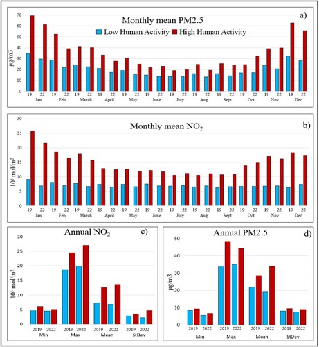
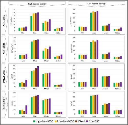
Figure 6. Annual min, max, mean, and StDev values for NO₂ and PM2.5 pollutants for various GSC classes over HHA and LHA regions.

4.4. Impact of GSC on air pollution

By computing yearly min, max, mean, and StDev values for each (see Section 3.1), we examined the effect of various GSC classes on NO₂ and PM2.5 concentrations over HHA and LHA regions. As shown in Figure 6, the NO₂ and PM2.5 rates in LHA regions were almost identical across all four classes, while in HHA regions, there was a significant variance in the rates. Regarding the temporal factor, 2019 saw more variety among the four groups than in 2022. Overall, across all calculated measures for 2019 and 2022 in both the HHA and LHA regions, the tall GSC class had the lowest pollutant concentration. In contrast, over HHA locations, the non-GSC class exhibited the highest concentrations of NO₂ and PM2.5.

Annual min and StDev values did not vary much among the four GSC classes, even though tall GSC had the lowest values across locations and years. For example, the tall GSC class had the lowest yearly min value of NO₂ pollutant with 5.2 × 10⁵ mol/m² in 2019 over HHA regions, while the highest annual min value of NO₂ pollutant belonged to the non-GS class with 6.9 × 10⁵ mol/m². On the other hand, the annual max and StDev, especially in the HHA region, showed the greatest differences across the four categories. For example, the tall GSC indicated an annual max PM2.5 value of 42 ug/m³ in 2019 in the HHA region, which was 10 and 16 ug/m³ lower than the short GSC and non-GSC classes.

Our investigation revealed that tall GSC contributes more than short GSC to air pollution reduction. As shown in Figure 6, in 2019 and 2022, tall GSC showed 9% and 4% lower average annual amounts of NO₂ over HHA regions, respectively, compared to short GSC class. Similarly, PM2.5 levels were 25% and 20% lower in the tall GSC. In terms of min and StDev values for NO₂ and PM2.5 in 2019 and 2022, both classes showed nearly equal trends, with the tall GSC class slightly outperforming. When it came to max NO₂ and PM2.5 values, the tall GSC class had lower PM2.5 levels, while the NO₂ values were nearly identical between the two classes.

5. Discussion

5.1. Air pollution retrieval using RS-based technology

Ground-based and RS-based methods are two primary ways to calculate air pollution. Ground-based approaches are the primary means of retrieving air pollution data. However, these techniques, which depend on a restricted quantity of weather stations, are laborious and costly. They also lack frequent records in constantly changing environments, such as urban areas. In contrast, the RS-based technology can estimate and monitor real-time air pollution at dense spatial sampling intervals.

Furthermore, RS-based methods can monitor large-scale areas, even in remote and hard-to-reach areas where the number of ground-based weather stations is often inadequate for a comprehensive assessment. This study used RS data, including Sentinel-5 TROPOMI sensor and MODIS AOD products, to map NO₂ and PM2.5 levels over Sichuan province in 2019 and 2022. We used the GEE platform to retrieve and process NO2 levels, which facilitated a quicker and smoother analysis procedure by incorporating image-based features, high-performance processing power and eliminating the need to download raw data (Ayyamperumal et al. 2024). Our accuracy assessment task using ground-based weather station data revealed reasonable accuracy for the obtained satellite-based NO₂ and PM2.5 values in both years. These findings confirm the efficiency of RS-based methods for studying air pollution, consistent with previous studies by Ayyamperumal et al. (2024), Kazemi Garajeh et al. (2023), Shami et al. (2022), and Ghasempour et al. (2021).

5.2. Spatial–temporal distribution of NO₂ and PM2.5 over Sichuan

The spatial–temporal variations in NO₂ and PM2.5 over Sichuan were analyzed in Section 4.1. Our analysis showed that regions with high amounts of NO₂ and PM2.5 were primarily in eastern Sichuan (Sichuan basin). The distinct landscape of Sichuan is the primary reason behind this. The Sichuan basin, illustrated in Figure 1(c), lies at a low elevation of only a few hundred meters above sea level and is enclosed by tall mountains exceeding 4000 meters in height. This geographical setup results in low wind speeds (Wang et al. 2018), elevated humidity levels (Hu and Wang 2021), and frequent fog formation (Ning et al. 2018), all of which contribute to increased air pollution levels. Our statistical analysis also revealed that January and December had the highest concentrations of PM2.5 and NO₂, whereas the months from April to September had the lowest concentrations of these two pollutants. Our findings are in line with Fang et al. 2021; Hu and Wang 2021; and Ning et al. 2018.

5.3. Impact of GSC on air pollution

The general theory suggests that GSC positively impacts air quality. Therefore, analyzing the evidence relating to GSC's impact on air pollution mitigation is critical. In this study, we classified GSC areas based on their height into two groups: tall GSC and short GSC. Our analysis revealed GSCs have lower NO₂ and PM2.5 levels over HHA regions than non-GSC areas. This can confirm the findings of prior studies that stated the positive impact of GSC on enhancing air quality (Lee, Tran, and Yu 2023; Linden et al. 2023).

Furthermore, we found that tall GSC exhibit lower pollutant amounts across all areas studied, indicating a potential correlation between GSC height and pollution mitigation efficacy. The higher impact of tall GSC than short GSC may be attributed to its superior shading and cooling capabilities compared to short GSC (Akbari et al., 1997; Selmi et al. 2016). These findings are in line with the findings of Taleghani et al. 2020, where they highlighted that short GSC (e.g. hedges) has less influence on reducing air pollution compared to tall GSC (e.g. trees) due to reduced wind speed.

Based on our results (Figure 6), over HHA regions, while tall GSC emerged as effective sinks for PM 2.5 compared to short GSC (25% and 20% lower average annual in 2019 and 2022, respectively), their performance in reducing NO₂ pollutant levels was relatively limited (9% and 4% lower average annual in 2019 and 2022, respectively). This illustrates that the impact of GSCs is different between particles and gaseous pollutants, which is in line with the findings of Wang, Chu, et al. (2022) and Wang, Guo, et al. (2022). A limited (nearly 7%) effect of GSC in reducing NO₂ levels has also been reported by Grundström and Pleijel (2014).

5.4. Limitation of this study

The literature has widely documented the successful application of satellite data for air pollution research (Ayyamperumal et al. 2024; Phan and Fukui 2024; Shami et al. 2022). However, no-data pixels can be an issue when studying large-scale regions (Ghasempour, Sekertekin, and Kutoglu 2021). Therefore, it is important to consider the potential noise or no-data issue while utilizing satellite-derived air pollution data. Additionally, the 1100 m resolution of the available satellite-derived air pollution data restricted us to only focusing on tall GSC and short GSC in this investigation. As a result, implementing downscaling techniques to generate higher-resolution air pollution data for future studies would be useful.

Following previous studies (Garajeh et al., 2023; Ghasempour, Sekertekin, and Kutoglu 2021; Shami et al. 2022), this work utilized data from ground stations to assess the accuracy of satellite-based air pollution data. One limitation of this approach is the sparse distribution and limited number of ground-based stations. Furthermore, satellite observations record air pollution data over the entire vertical extent of the atmosphere, while ground stations only monitor these pollutants at the surface level. Therefore, it is important to acknowledge that the accuracy assessment using ground station data might include a potential bias.

In this study, we focused exclusively on the years 2019 (before the COVID outbreak) and 2022 (after the COVID outbreak) to mitigate COVID restrictions’ impact on our analysis. However, we should note that COVID-19 continued to plague the year 2022, preventing the economy and human activity from returning to the levels seen in 2019. Furthermore, we employed vegetation height as a criterion to classify GSCs into several categories in this work. Future research will compare various GSC classification systems, such as vegetation kinds, leaf area density, and canopy cover, for air pollution monitoring.

6. Conclusion

Air pollution is the greatest health risk to human health; as a result, the United Nations has incorporated it into several SDGs. The positive impact of GSC on improving air quality has been of particular interest. However, prior studies mainly concentrated on small-scale studies at the city or district level, whereas RS data provides a significant possibility for large-scale investigations. Here, we used RS-based satellite data to study the impact of various GSC classes on two key air pollution indicators in Sichuan Province between 2019 and 2022. This study confirmed the possibility of conducting air pollution studies over large and hard-to-reach areas using RS technology. Our analysis showed that HHA in the Sichuan Province was nearly twice as polluted as the LHA regions. Additionally, we found that GSC areas generally had lower NO₂ and PM2.5 concentrations than non-GSC areas. The tall GSC class appeared to have the lowest air pollution amounts compared to the short GSC class. The research framework outlined in this paper is applicable across various geographical areas, ensuring extensive practical efficacy in mitigating air pollution and promoting sustainable development. Additionally, our findings regarding the effects of GSC types can contribute to developing effective green infrastructure initiatives by informing urban planning and environmental policies.

CRediT authorship contribution statement

Amin Naboureh: Conceptualization, Methodology, Software, Data Curation, Writing – original draft, Funding acquisition. Ainong Li and Jinhu Bian: Conceptualization, Supervision, Writing – review & editing. Guangbin Lei, Xi Nan, and Zhengjian Zhang: Data Curation, Validation, and Formal analysis. Sivash Shami: Software, Validation, and formal analysis. Lin Xiaohan: Data Curation and Formal analysis.

Disclosure statement

No potential conflict of interest was reported by the author(s).

Data availability statement

Landsat-8 and satellite-based NO2 data are accessible for free download at https://developers.google.com/earth-engine/datasets; PM 2.5 data is also publicly available at https://weijing-rs.github.io/product.html. The ground-based NO₂ and PM2.5 provided by the China national environmental monitoring center is available at http://www.cnemc.cn/.

Additional information

Funding

This work was supported by the National Natural Science Foundation project of China under Grants U23A2019, 42090015, 42171382, and 42271398; the Sichuan province key research and development project under Grant 2023YFWZ0007; the National Key Research and Development Program of China under Grant 2020YFA0608702; and the Science and Technology Research Program of Institute of Mountain Hazards and Environment, Chinese Academy of Sciences Under Grant IMHE-CXTD-03.

References

- Akbari, H., D. M. Kurn, S. E. Bretz, and J. W. Hanford. 1997. “Peak power and cooling energy savings of shade trees.” Energy and buildings 25 (2): 139–148.
- Ayyamperumal, R., A. Banerjee, Z. Zhang, Nusrat Nazir, Fengjie Li, Chengjun Zhang, and X. Huang. 2024. “Quantifying Climate Variation and Associated Regional air Pollution in Southern India Using Google Earth Engine.” Science of the Total Environment 909:168470. https://doi.org/10.1016/j.scitotenv.2023.168470.
- Barwise, Y., and P. Kumar. 2020. “Designing Vegetation Barriers for Urban air Pollution Abatement: A Practical Review for Appropriate Plant Species Selection.” Npj Climate and Atmospheric Science 3 (1): 12. https://doi.org/10.1038/s41612-020-0115-3.
- Bian, J., A. Li, G. Lei, Zhengjian Zhang, and Xi Nan. 2020. “Global High-Resolution Mountain Green Cover Index Mapping Based on Landsat Images and Google Earth Engine.” ISPRS Journal of Photogrammetry and Remote Sensing 162:63–76. https://doi.org/10.1016/j.isprsjprs.2020.02.011.
- Diener, A., and P. Mudu. 2021. “How Can Vegetation Protect us from air Pollution? A Critical Review on Green Spaces' Mitigation Abilities for air-Borne Particles from a Public Health Perspective - with Implications for Urban Planning.” Science of the Total Environment 796:148605. https://doi.org/10.1016/j.scitotenv.2021.148605.
- Ebrahimy, H., A. Naboureh, B. Feizizadeh, J. Aryal, and O. Ghorbanzadeh. 2021. “Integration of Sentinel-1 and Sentinel-2 Data with the G-SMOTE Technique for Boosting Land Cover Classification Accuracy.” Applied Sciences 11 (21): 10309. https://doi.org/10.3390/app112110309.
- Fang, C., X. Tan, Y. Zhong, and J. Wang. 2021. “Research on the Temporal and Spatial Characteristics of air Pollutants in Sichuan Basin.” Atmosphere 12 (11): 1504. https://doi.org/10.3390/atmos12111504.
- Fuller, R., P. J. Landrigan, K. Balakrishnan, Glynda Bathan, Stephan Bose-O'Reilly, Michael Brauer, Jack Caravanos, et al. 2022. “Pollution and Health: A Progress Update.” The Lancet Planetary Health 6 (6): e535–e547. https://doi.org/10.1016/S2542-5196(22)00090-0.
- Ghasempour, F., A. Sekertekin, and S. H. Kutoglu. 2021. “Google Earth Engine Based Spatio-Temporal Analysis of air Pollutants Before and During the First Wave COVID-19 Outbreak Over Turkey via Remote Sensing.” Journal of Cleaner Production 319:128599. https://doi.org/10.1016/j.jclepro.2021.128599.
- Gong, P., X. Li, J. Wang, Yuqi Bai, Bin Chen, Tengyun Hu, Xiaoping Liu, et al. 2020. “Annual Maps of Global Artificial Impervious Area (GAIA) Between 1985 and 2018.” Remote Sensing of Environment 236:111510. https://doi.org/10.1016/j.rse.2019.111510.
- Gorelick, N., M. Hancher, M. Dixon, Simon Ilyushchenko, David Thau, and Rebecca Moore. 2017. “Google Earth Engine: Planetary-Scale Geospatial Analysis for Everyone.” Remote Sensing of Environment 202:18–27. https://doi.org/10.1016/j.rse.2017.06.031.
- Grundström, M., and H. Pleijel. 2014. “Limited Effect of Urban Tree Vegetation on NO2 and O3 Concentrations Near a Traffic Route.” Environmental Pollution 189:73–76. https://doi.org/10.1016/j.envpol.2014.02.026.
- Guo, H., L. Huang, L. Luo, J. Liu, and X. Li. 2023. “Progress on achieving environmental SDGs assessed from Big Earth Data in China.” Science Bulletin 68 (24): 3129–3132.
- Guo, Q., D. Wu, C. Yu, Tianshuang Wang, Mingxia Ji, and X. Wang. 2022. “Impacts of Meteorological Parameters on the Occurrence of air Pollution Episodes in the Sichuan Basin.” Journal of Environmental Sciences 114:308–321. https://doi.org/10.1016/j.jes.2021.09.006.
- Hu, Y., and S. Wang. 2021. “Formation Mechanism of a Severe air Pollution Event: A Case Study in the Sichuan Basin, Southwest China.” Atmospheric Environment 246:118135. https://doi.org/10.1016/j.atmosenv.2020.118135.
- Huang, Z., H. Fan, and L. Shen. 2019. “Case-based Reasoning for Selection of the Best Practices in low-Carbon City Development.” Frontiers of Engineering Management 6 (3): 416–432. https://doi.org/10.1007/s42524-019-0036-1.
- Ialongo, I., H. Virta, H. Eskes, Jari Hovila, and J. Douros. 2020. “Comparison of TROPOMI/Sentinel-5 Precursor NO 2 Observations with Ground-Based Measurements in Helsinki.” Atmospheric Measurement Techniques 13 (1): 205–218. https://doi.org/10.5194/amt-13-205-2020.
- Imani, M. 2021. “Particulate Matter (PM2.5 and PM10) Generation map Using MODIS Level-1 Satellite Images and Deep Neural Network.” Journal of Environmental Management 281:111888. https://doi.org/10.1016/j.jenvman.2020.111888.
- Kazemi Garajeh, M., G. Laneve, H. Rezaei, M. Sadeghnejad, N. Mohamadzadeh, B. Salmani. 2023. “Monitoring trends of CO, NO2, SO2, and O3 pollutants using time-series sentinel-5 images based on google earth engine.” Pollutants 3 (2): 255–279.
- Kinney, P. L. 2018. “Interactions of Climate Change, air Pollution, and Human Health.” Current Environmental Health Reports 5:179–186. https://doi.org/10.1007/s40572-018-0188-x.
- La Nauze, A., and E. R. Severnini. 2021. Air Pollution and Adult Cognition: Evidence from Brain Training (No. w28785). Cambridge, MA: National Bureau of Economic Research.
- Lee, W. S., T. M. Tran, and L. B. Yu. 2023. “Green Infrastructure and air Pollution: Evidence from Highways Connecting two Megacities in China.” Journal of Environmental Economics and Management 122:102884. https://doi.org/10.1016/j.jeem.2023.102884.
- Li, J., and X. Huang. 2020. “Impact of land-cover layout on particulate matter 2.5 in urban areas of China.” International Journal of Digital Earth.
- Linden, J., M. Gustafsson, J. Uddling, Ågot Watne, and H. Pleijel. 2023. “Air Pollution Removal Through Deposition on Urban Vegetation: The Importance of Vegetation Characteristics.” Urban Forestry & Urban Greening 81:127843. https://doi.org/10.1016/j.ufug.2023.127843.
- Liu, L., Y. Chen, T. Wu, and H. Li. 2018. “The Drivers of air Pollution in the Development of Western China: The Case of Sichuan Province.” Journal of Cleaner Production 197:1169–1176. https://doi.org/10.1016/j.jclepro.2018.06.260.
- Longley, M., P. C. Jepson, J. Izquierdo, and N. Sotherton. 1997. “Temporal and spatial changes in aphid and parasitoid populations following applications of deltamethrin in winter wheat.” Entomologia Experimentalis et Applicata 83 (1): 41–52.
- Naboureh, A., J. Bian, G. Lei, and A. Li. 2021. “A Review of Land use/Land Cover Change Mapping in the China-Central Asia-West Asia Economic Corridor Countries.” Big Earth Data 5 (2): 237–257. https://doi.org/10.1080/20964471.2020.1842305.
- Naboureh, A., A. Li, J. Bian, G. Lei, and X. Nan. 2023. “Land Cover Dataset of the China Central-Asia West-Asia Economic Corridor from 1993 to 2018.” Scientific Data 10 (1): 728. https://doi.org/10.1038/s41597-023-02623-z.
- Ning, G., S. Wang, S. H. L. Yim, Jixiang Li, Yuling Hu, Ziwei Shang, Jinyan Wang, and Jiaxin Wang. 2018. “Impact of low-Pressure Systems on Winter Heavy air Pollution in the Northwest Sichuan Basin, China.” Atmospheric Chemistry and Physics 18 (18): 13601–13615. https://doi.org/10.5194/acp-18-13601-2018.
- Peeples, L. 2020. “How air Pollution Threatens Brain Health.” Proceedings of the National Academy of Sciences 117 (25): 13856–13860. https://doi.org/10.1073/pnas.2008940117.
- Phan, Anh, and Hiromichi Fukui. 2024. “Unusual Response of O3 and CH4 to NO2 Emissions Reduction in Japan During the COVID-19 Pandemic.” International Journal of DigitalEarth 17 (1): 2297844.
- Rabiei-Dastjerdi, H., S. Mohammadi, and M. Saber. 2022. “Spatiotemporal Analysis of NO2 Production Using TROPOMI Time-Series Images and Google Earth Engine in a Middle Eastern Country.” Remote Sensing 14 (7): 1725. https://doi.org/10.3390/rs14071725.
- Rentschler, J., and N. Leonova. 2023. “Global air Pollution Exposure and Poverty.” Nature Communications 14 (1): 4432. https://doi.org/10.1038/s41467-023-39797-4.
- Selmi, W., C. Weber, E. Rivière, Nadège Blond, Lotfi Mehdi, and D. Nowak. 2016. “Air Pollution Removal by Trees in Public Green Spaces in Strasbourg City, France.” Urban Forestry & Urban Greening 17:192–201. https://doi.org/10.1016/j.ufug.2016.04.010.
- Shami, S., B. Ranjgar, J. Bian, Mahdi Khoshlahjeh Azar, Armin Moghimi, Meisam Amani, Amin Naboureh, and A. Naboureh. 2022. “Trends of CO and NO2 Pollutants in Iran During COVID-19 Pandemic Using Timeseries Sentinel-5 Images in Google Earth Engine.” Pollutants 2 (2): 156–171. https://doi.org/10.3390/pollutants2020012.
- Singh, M., B. B. Singh, R. Singh, Badimela Upendra, Rupinder Kaur, Sukhpal Singh Gill, and M. S. Biswas. 2021. “Quantifying COVID-19 Enforced Global Changes in Atmospheric Pollutants Using Cloud Computing Based Remote Sensing.” Remote Sensing Applications: Society and Environment 22:100489. https://doi.org/10.1016/j.rsase.2021.100489.
- Soleimanpour, M., O. Alizadeh, and S. Sabetghadam. 2023. “Analysis of Diurnal to Seasonal Variations and Trends in air Pollution Potential in an Urban Area.” Scientific Reports 13 (1): 21065. https://doi.org/10.1038/s41598-023-48420-x.
- Taleghani, M., A. Clark, W. Swan, and A. Mohegh. 2020. “Air Pollution in a Microclimate; the Impact of Different Green Barriers on the Dispersion.” Science of the Total Environment 711:134649. https://doi.org/10.1016/j.scitotenv.2019.134649.
- Taylor, L., and D. F. Hochuli. 2017. “Defining Greenspace: Multiple Uses Across Multiple Disciplines.” Landscape and Urban Planning 158:25–38. https://doi.org/10.1016/j.landurbplan.2016.09.024.
- Wang, S., H. Chu, C. Gong, Ping Wang, Fei Wu, and Chunhong Zhao. 2022. “The Effects of COVID-19 Lockdown on air Pollutant Concentrations Across China: A Google Earth Engine-Based Analysis.” International Journal of Environmental Research and Public Health 19 (24): 17056. https://doi.org/10.3390/ijerph192417056.
- Wang, X., R. E. Dickinson, L. Su, Chunlüe Zhou, and K. Wang. 2018. “PM2.5 Pollution in China and How It Has Been Exacerbated by Terrain and Meteorological Conditions.” Bulletin of the American Meteorological Society 99 (1): 105–119. https://doi.org/10.1175/BAMS-D-16-0301.1.
- Wang, C., M. Guo, J. Jin, Yifan Yang, Yujie Ren, Yang Wang, and J. Cao. 2022. “Does the Spatial Pattern of Plants and Green Space Affect air Pollutant Concentrations? Evidence from 37 Garden Cities in China.” Plants 11 (21): 2847. https://doi.org/10.3390/plants11212847.
- Wei, J., Z. Li, M. Cribb, Wei Huang, Wenhao Xue, Lin Sun, Jianping Guo, et al. 2020. “Improved 1 km Resolution PM2.5 Estimates Across China Using Enhanced Space-Time Extremely Randomized Trees.” Atmospheric Chemistry and Physics 20:3273–3289. https://doi.org/10.5194/acp-20-3273-2020.
- Wei, J., Z. Li, A. Lyapustin, Lin Sun, Yiran Peng, Wenhao Xue, Tianning Su, and M. Cribb. 2021. “Reconstructing 1-km-Resolution High-Quality PM2.5 Data Records from 2000 to 2018 in China: Spatiotemporal Variations and Policy Implications.” Remote Sensing of Environment 252:112136. https://doi.org/10.1016/j.rse.2020.112136.
- Wu, Xiaobo, Xiaoyu Fan, Xiaojing Liu, Lin Xiao, Qimin Ma, Qimin He, Sizhuo Gao, and Yuting Qiao. 2023. “Temporal and Spatial Variations of Ecological Quality of Chengdu-Chongqing Urban Agglomeration Based on Google Earth Engine Cloud Platform.” Chinese Journal of Ecology 42 (3): 759.
- Xiao, Q., Z. Ma, S. Li, and Y. Liu. 2015. “The impact of winter heating on air pollution in China.” PloS one 10 (1): e0117311.
- Xu, T., C. Zhang, C. Liu, and Q. Hu. 2023. “Variability of PM2. 5 and O3 concentrations and their driving forces over Chinese megacities during 2018-2020.” Journal of Environmental Sciences 124: 1–10.
- Yang, Q., Q. Yuan, and T. Li. 2022. “Ultrahigh-resolution PM2.5 Estimation from top-of-Atmosphere Reflectance with Machine Learning: Theories, Methods, and Applications.” Environmental Pollution 306:119347. https://doi.org/10.1016/j.envpol.2022.119347.
- Yuan, L., K. Shin, and S. Managi. 2018. “Subjective Well-Being and Environmental Quality: The Impact of air Pollution and Green Coverage in China.” Ecological Economics 153:124–138. https://doi.org/10.1016/j.ecolecon.2018.04.033.
- Zhang, Z., A. Arshad, C. Zhang, S. Hussain, and W. Li. 2020. “Unprecedented Temporary Reduction in Global air Pollution Associated with COVID-19 Forced Confinement: A Continental and City Scale Analysis.” Remote Sensing 12 (15): 2420. https://doi.org/10.3390/rs12152420.
- Zhang, Q., Y. Zheng, D. Tong, Min Shao, Shuxiao Wang, Yuanhang Zhang, Xiangde Xu, et al. 2019. “Drivers of Improved PM2. 5 air Quality in China from 2013 to 2017.” Proceedings of the National Academy of Sciences 116 (49): 24463–24469. https://doi.org/10.1073/pnas.1907956116.
- Zhong, J., Z. Li, Z. Sun, Yangjie Tian, and F. Yang. 2020. “The Spatial Equilibrium Analysis of Urban Green Space and Human Activity in Chengdu, China.” Journal of Cleaner Production 259:120754. https://doi.org/10.1016/j.jclepro.2020.120754.
- Zhou, K., Y. Zhao, L. Zhang, and M. Xi. 2021. “Declining dry Deposition of NO2 and SO2 with Diverse Spatiotemporal Patterns in China from 2013 to 2018.” Atmospheric Environment 262:118655. https://doi.org/10.1016/j.atmosenv.2021.118655.
- Zhu, J., Y. Zhai, S. Feng, Ya Tan, and W. Wei. 2022. “Trade-offs and Synergies among air-Pollution-Related SDGs as Well as Interactions Between air-Pollution-Related SDGs and Other SDGs.” Journal of Cleaner Production 331:129890. https://doi.org/10.1016/j.jclepro.2021.129890.