A vision-aided RTK ambiguity resolution method by map lane matching for intelligent vehicle in urban environment

ABSTRACT

Despite the high-precision performance of GNSS real-time kinematic (RTK) in many cases, harsh signal environments still lead to ambiguity-fixed failure and worse positioning results in kinematic localization. Intelligent vehicles are equipped with cameras for perception. Visual measurements can add new information to satellite measurements, thus improving integer ambiguity resolution (AR). Given road lane lines are stationary and their accurate positions can be previously acquired, we encode the lane lines with rectangles and integrate them into a commonly used map format. Considering the ambiguous and repetitive land lines, a map-based ambiguous lane matching method is proposed to find all possible rectangles where a vehicle may locate. And a vision-based relative positioning is then applied by measuring the relative position between the lane line corner and the vehicle. Finally, the two results are introduced into RTK single-epoch AR to find the most accurate ambiguity estimations. To extensively evaluate our method, we compare it with a tightly integrated system of GNSS/INS (GINS) and a well-known tightly coupled GNSS-Visual-Inertial fusion system (GVINS) in simulated urban environments and a real dense urban environment. Experimental results prove the superiority of our method over GINS and GVINS in success rates, fixed rates and pose accuracy.

KEYWORDS:

• GNSS RTK
• ambiguity resolution
• GNSS/INS/Vision integration
• map lane matching

1. Introduction

High-precision positioning plays a key role in intelligent vehicles which normally uses GNSS RTK technology to localize the vehicles. RTK can achieve centimeter-level positioning accuracy if integer carrier ambiguity is resolved (Zhang et al. 2019). Intelligent vehicles require real-time high-precision localization to operate safely, which means the integer ambiguity must be fixed correctly and instantaneously with a single epoch of observation, which is known as ambiguity resolution (AR). Single-epoch AR is normally resolved by forming the combination of multi-frequency multi-GNSS observations (Li, Qin, and Liu 2019; Psychas, Verhagen, and Teunissen 2020; Zhang and He 2016). For example, the Hatch–Melbourne–Wübbena combination of dual-frequency signals in TurboEdit algorithm (Blewitt 1990), and the extra-wide-lane and wide-lane combinations of triple-frequency signals (de Lacy, Reguzzoni, and Sansò 2012; Li et al. 2016). Deng et al. investigated both loose and tight combinations of current four GNSSs and concluded that loose combination achieved much lower ambiguity fixing rates than tight combination when the satellite signals are severely obstructed (Deng et al. 2020). Additionally, Odolinski et al. compared single-epoch performance of single frequency with dual-system (SF-DS) and dual-frequency with single-system (DS-SS) and indicated that SF-DS had potential to achieve comparable AR performance to that of sDS-SS, even with low-cost receivers (Odolinski and Teunissen 2016). He et al. draw similar conclusion by evaluating the performance of single- and dual-frequency BDS+GPS single-epoch kinematic positioning (He et al. 2014). However, single-epoch RTK may fail in AR or fix ambiguity incorrectly in GNSS-challenged environments (Carcanague 2012), e.g. urban canyon. Therefore, we aim to improve single-epoch AR performance in the urban environments in this work.

Other than GNSS receiver, intelligent vehicles usually install many other sensors, like MEMS-IMU, camera and so on. MEMS-IMU can be tightly coupled with GNSS to aid AR (El-Sheimy 2004; El-Sheimy and Youssef 2020). Li et al. developed the tightly coupled single-frequency-multi-GNSS-RTK/MEMS-IMU integration to improve AR and positioning performance for short baselines in urban environments (Li et al. 2017; Li, Zhang et al. 2018). Zhu et al. also proposed a low-cost MEMS-IMU and RTK tightly coupled scheme considering a vehicle kinematics constraint (Zhu et al. 2019). Gao et al. investigated tight integration of the multi-GNSS single-frequency observations and MEMS-IMU measurements to alleviate the effect of the ionospheric delay and receiver differential code bias on AR and positioning (Gao et al. 2017). However, MEMS-IMU can only keep high accuracy for a short while because of its large time-dependent drift errors when GNSS is not available.

For autonomous driving, a camera can be used for localization using visual Simultaneous Localization and Mapping (vSLAM) technique. Some research integrated GNSS, INS and vSLAM to provide more accurate position than GNSS-only or camera-only navigation by Kalman filter (Tao et al. 2017; Yan et al. 2018), Particle filter (Shunsuke, Yanlei, and Hsu 2015; Suhr et al. 2016) or graph-based optimization (Gong et al. 2020; Li et al. 2021; Niu et al. 2022; Wen et al. 2020). However, the visual measurements did not contribute to AR in these works, since they fused position from vSLAM with GNSS and INS directly. Liu et al. developed a tight GNSS/INS/vSLAM framework based on a centralized Kalman filter (Li et al. 2022; Liu 2018). INS-aided feature position estimation in vSLAM was introduced into the state update which included carrier phase ambiguity. A broadly used open-source framework for GNSS-Visual-INS (GVINS) integration was released in 2022 (Cao, Lu, and Shen 2022), in which the GNSS code pseudorange and Doppler shift measurements, along with visual and inertial information, were modeled and used to constrain the system states in a factor graph framework. But above works either neglected GNSS phase measurements or only estimated float ambiguities rather than fixing them to integer values by AR to achieve high-precision position. Besides, vSLAM may accumulate drift errors over running distances, which may reduce the accuracy of ambiguity estimation.

Except for vSLAM techniques based on feature detection and feature association, visual lane-marking detection provides another way to assist ego-lane estimation for vehicles using a prior map (Pöppl et al. 2023). Rabe et al. calculated the visually observed distances and angles to lane markings and corrected the lateral position (position relative to the road boundary) of a vehicle based on a map (Rabe et al. 2017; Rabe, Necker, and Stiller 2016). Kasmi et al. adopted a similar visually lateral positioning module in an end-to-end probabilistic ego-vehicle localization framework (Kasmi et al. 2020). The longitudinal position along the road was determined by GNSS in their works, and its precision depends on GNSS positioning condition. Xiao et al. pre-collected information of the road landmarks and stored it in a self-defined map and then matched geometric features detected from visual frames against the map to localize a vehicle in the map (Xiao et al. 2018; Xiao et al. 2020). Lu et al. formulated a non-linear optimization to match the road markings with the map (Lu et al. 2017; Qin et al. 2021). If there is a sufficient number of marking patches, the map-based positioning method may work well, but it may fail in regions where marking patches are repetitive and homogeneous (Schreiber, Knöppel, and Franke 2013). Moreover, it appears that few researchers focused on tightly coupling the visual map-based positioning method and GNSS AR.

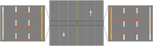
In many cases, lane line is not solid but dashed line, and we take advantage of this nature and encode the lane lines as continuous rectangles with same sizes, as shown in Figure 1. Hence, on a multi-lane road, longitudinally and laterally positioning a vehicle becomes finding the correct rectangle in which the vehicle is located. The main contributions of this article can be summarized as follows:

1. We design an encoding method for lane lines and integrate this encoding scheme with the widely used map format called lanelet, which provides a way for coupling the map data and GNSS raw measurements.

2. We proposed a tightly integrated framework for map-based positioning, vision-based relative positioning, GNSS and MEMS-IMU raw measurements, which improves GNSS AR performance and positioning accuracy.

3. To deal with the map-based positioning uncertainty caused by repetitive and homogeneous lane lines, an ambiguous lane matching method is proposed by considering all possible rectangles that a vehicle may locate in. And then all the rectangles information from the map and visual relative positioning results are combined as virtual observations and incorporated into the process of GNSS-RTK AR. Finally, the position result with the largest ratio value is chosen as the final position estimation.

Figure 1. Encoding lanes with orange rectangles of same sizes on a multi-lane road. Ends of each stroke of dashed lane lines along the direction of velocity are extracted (denoted as red dots in the left and right subfigures, called as ‘stroke end (SE)’ in the following texts). Rectangles are defined by two or four SEs.

2. Methodology

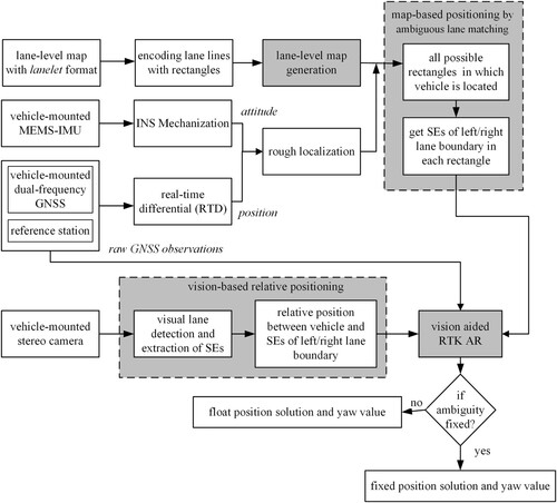
A prior map should be generated before on-line localization. We follow close to the map format of lanelet (Bender, Ziegler, and Stiller 2014), and integrate our lane-line-encoding scheme with lanelet format. Based on an approximate position of vehicle, all possible rectangles that the vehicle may locate in are found by ambiguous lane matching. The rectangle information and the vision-based relation positioning information are then used to assist GNSS-RTK AR. To fix ambiguity, the Least-squares AMBiguity Decorrelation Adjustment (LAMBDA) (Teunissen, De Jonge, and Tiberius 1995) was used in our work. Figure 2 shows the flowchart of our integrated system for a single epoch.

Figure 2. Flowchart of our integrated system. Methods with gray background will be introduced in details in following texts.

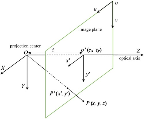
In our work, we define the WGS-84 ECEF reference as e-frame, the local Cartesian coordinate frame (g-frame) as east–north–up with origin at GNSS RTK reference station center, the navigation frame (n-frame) as east–north–up with origin at IMU center, the body frame (b-frame) is centered at IMU center with front–right–down. Figure 3 shows the pinhole camera model which defines the camera coordinate frame (c-frame), the image coordinate frame (im-frame) and the pixel coordinate frame (pi-frame). b-frame and c-frame are pre-calibrated to achieve time and spatial synchronization.

Figure 3. Illustration of pinhole camera model. f is the focal length, O-XYZ is the camera coordinate frame, o’-x’y’ is the image coordinate frame, and o-uv is the pixel coordinate frame. P is a point in the three-dimensional space with coordinate (x, y, z) in O-XYZ and coordinate (x’, y’) in o’-x’y’.

3. Lane-level map generation

Lanelets is a high-definition map framework for autonomous driving, which is based on atomic lane sections (called as lanelet). In this work, we use the geometrical and topological aspects of lanelet. Each lanelet is characterized by two polylines as left and right boundaries that are made up of a series of discrete points with latitude and longitude information. Both left and right boundaries include a start point and an end point. More details about lanelet can be seen in Bender, Ziegler, and Stiller (2014). Topological information such as neighboring and succeeding lanelet can be determined by comparing lanelet boundaries. We use this information to determine the number of total parallel lanes in a multi-lane road segment.

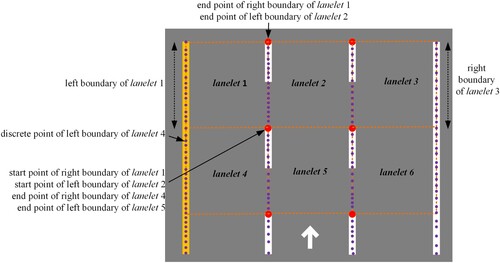
In the lanelet map framework, the types of lane lines are not considered. In our work, we encode the lanes with rectangles as Figure 1. To make the map available for our method, lanelet is tagged with a ‘SE’ attribution by overlapping the lanelet with rectangles and making SEs as start points or end points of boundaries of lanelet, shown in Figure 4. The data of the map are acquired by a data-collection vehicle equipped with high-precision positioning and perception sensors. All map data are stored in the e-frame as an XML file. The map is introduced to our system by loading the XML file.

Figure 4. Format of the map used in our work. Each orange rectangle (defined in Figure 1) is overlapping with a lanelet. The purple points are discrete points of boundaries of lanelets. If there are SEs (red dots) on the boundaries, we make SEs as start point or end point of the boundaries of lanelet.

4. Map-based positioning by ambiguous lane matching

Meter-level positioning accuracy of GNSS real-time differential (RTD) in urban environments cannot satisfy the high-precision requirements of self-driving vehicle. But it provides a good guess of the true position. Based on the approximate position from GNSS RTD and attitude from INS mechanization, we search for all possible positions on the map. To make the spatial search in a lanelet map more efficient, R-tree is used to organize the map data. First, the map is quired using the approximate position to find the lanelet where vehicle approximately locates by taking advantage of cross product as lanelets are convex polygons. If multiple lanelets are calculated, for example in intersections, we calculate the angle difference between the yaw angle from INS and the orientations of the lanelets. The most likely lanelet $L{L}_{\mathrm{RTD}}$ is determined with the smallest angle difference. The orientation of lanelet is calculated by finding four closest points to the vehicle in the left boundary and best-line fitting the points. The orientation of the fitting line is assumed to be the orientation of the lanelet.

Based on $L{L}_{\mathrm{RTD}}$, all possible lanelets (or rectangles) are then searched on the map by ambiguous lane matching. The topological information in the lanelet-formatted map, such as neighboring and succeeding lanelets can be determined by comparing lanelet boundaries, can make our searching quite efficient. Given positioning errors in RTD, we define a searching ambiguity $N_{\mathrm{LL}}$ on the map. $L{L}_{\mathrm{RTD}}$ may have $n_x$ parallel lanes. $n_y$ lanelets are chosen in the longitudinal direction for each lane, and $N_{\mathrm{LL}}=n_x\cdot n_y$. An example is shown in Figure 5. $N_{\mathrm{LL}}$ can be freely adjusted based on the observation conditions of GNSS to consider large RTD positioning errors. From the $N_{\mathrm{LL}}$ possible lanelets, we can get $N_{\mathrm{LL}}$ SEs from the $N_{\mathrm{LL}}$ lanelets, denoted as $\left\{\right(x_{\mathrm{SE}1}^e,y_{\mathrm{SE}1}^e,z_{\mathrm{SE}1}^e),(x_{\mathrm{SE}2}^e,y_{\mathrm{SE}2}^e,z_{\mathrm{SE}2}^e),\dots ,(x_{\mathrm{SE}{N}_{\mathrm{LL}}}^e,y_{\mathrm{SE}{N}_{\mathrm{LL}}}^e,z_{\mathrm{SE}{N}_{\mathrm{LL}}}^e\left)\right\}$. For each lanelet, if both left and right boundaries have SEs as end points, the SE of left boundary is chosen. For example, in Figure 5, the SE of right boundary as end point is chosen in lanelet 1, but in lanelet 2 the SE of left boundary as end point is chosen. The positions of SEs in the e-frame are transformed to the g-frame by (1) $\left[\begin{array}{c}{x}_{\mathrm{SE}}^g\\ y_{\mathrm{SE}}^g\\ z_{\mathrm{SE}}^g\end{array}\right]=C_e^g\left[\begin{array}{c}{x}_{\mathrm{SE}}^e\text{-}{x}_0^e\\ y_{\mathrm{SE}}^e\text{-}{y}_0^e\\ z_{\mathrm{SE}}^e\text{-}{z}_0^e\end{array}\right],\mathrm{with}{C}_e^g=\left[\begin{array}{c}-\sin l_0-\sin b_0\cos l_0\cos b_0\cos l_0\\ \cos l_0-\sin b_0\sin l_0\cos b_0\sin l_0\\ 0\cos b_0\sin b_0\end{array}\right]$(1) where $b_0$, $l_0$, $x_0^e$, $y_0^e$, $z_0^e$ are the coordinate of reference station in the e-frame.

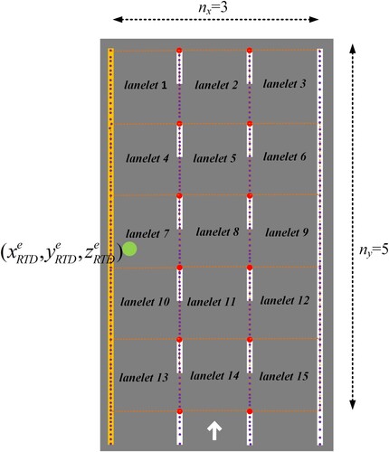
Figure 5. Green dot means the approximate position of vehicle from RTD. lanelet 7 is the lanelet $L{L}_{\mathrm{RTD}}$ where the RTD position locates. The searching ambiguity $N_{\mathrm{LL}}$ is 15 with 3 parallel lanes and 5 possibilities in the longitudinal direction. The 15 lanelets are assumed to be the possible lanelets where the true position of the vehicle locates.

5. Vision-based relative positioning

To achieve three-dimensional coordinates of SEs in the n-frame from the image, stereo vision is used in our work. Stereo rectification is used to make the im-frames of the two cameras coplanar and rows are aligned in their pi-frames. The intrinsic parameters of the left and right cameras are the same and using factory parameters, and the extrinsic parameters include a rotation matrix and a translation from the right camera to the left camera as the left camera is the main camera.

For the left image, a fast visual ego-lane detection method with lane width constraint is used as described in our previous work (Li, Zhou, et al. 2018). This method was proved to be robust and accurate while met real-time requirement. Here a brief introduction is described. To detect lane lines in the near-vehicle region efficiently, region of interest (ROI) is first initialized based on vanishing point, which is selected by an error model of the ${\theta }_c$: (2) $\delta \left(s\right)={\displaystyle \frac{w}{h}(\mathrm{fcos}{\theta }_c+\mathrm{ysin}{\theta }_c)\delta {\theta }_c}$(2) where $h$ is the height of camera from camera center to the road in the e-frame, $f$ is the focal length, y is the y coordinate in the c-frame, ${\theta }_c$ is the pitch angle of camera, $\delta {\theta }_c$ is the pitch error, $s$ is the width of lane markings in the im-frame and $w$ is that in the c-frame. ROI is produced by calculating a minimal row number $r_{min}$ in the pi-frame: (3) $r_{min}={\displaystyle \frac{\mathrm{fsin}{\theta }_c-\mathrm{lfcos}{\theta }_c\delta {\theta }_c}{\mathrm{lsin}{\theta }_c\delta {\theta }_c+\mathrm{fcos}{\theta }_c}\mathrm{with}l={\displaystyle \frac{\zeta +1}{\zeta -1}}}$(3) where $\zeta$ is a value that defines how many times the noisy lane width exceeds the actual width. Edge detection of lane lines is conducted in the ROI by calculating the gradient of each pixel in the pi-frame as (4) $E\left(i\right)=-\sum _{k=-w}^{-1}I(i+k)+\sum _{k=1}^{w}I(i+k)$(4) where i means the ith pixel, E means gradient, I is pixel value. Pixels with pairs of peak and valley gradient are selected as candidate edge points of lane lines. Then Hough Transform (HT) is used to detect candidate line segments. More details about HT can be referred to Saudi et al. (2008).

Line segments that locate on the left side and near the bottom of the image are chosen as our target line segment. The upper end of the target line segment in the image is extracted as the target SE with coordinate (u, v) in the pi-frame of the left camera.

To transform (u, v) in the pi-frame to $(x^c,y^c,z^c)$ in the c-frame, the parallax d at (u, v) is calculated from a disparity map which is generated from the left and right images (Zhang, Ai, and Dahnoun 2013), and the z-coordinate of SE in the c-frame $z^c$ is calculated as (5) $z^c={\displaystyle \frac{\mathrm{fb}}{d}}$(5) where b is the length of baseline of the stereo camera. x- and y-coordinates of SE in the c-frame $(x^c,y^c)$ can be obtained by (6) $z_c\left(\begin{array}{c}u\\ v\\ 1\end{array}\right)=\left(\begin{array}{ccc}\mathrm{\alpha f}& 0& c_x\\ 0& \text{β}f& c_y\\ 0& 0& 1\end{array}\right)\left(\begin{array}{c}{x}^c\\ y^c\\ z^c\end{array}\right)$(6) where $\alpha$ and $\text{β}$ are scale factor of x- and y-axes from the im-frame to the pi-frame, $c_x$ and $c_y$ are x- and y-coordinates in the pi-frame of the origin of im-frame. According to attitude information and lever arm of the left camera $(l_x,l_y,l_z)$, $(x^c,y^c,z^c)$ is transformed to the n-frame: (7) $\left[\begin{array}{c}{x}^n\\ y^n\\ z^n\end{array}\right]=C_b^n{C}_c^b\left[\begin{array}{c}{x}^c+l_x\\ y^c+l_y\\ z^c+l_z\end{array}\right],\mathrm{with}{C}_b^n=\left[\begin{array}{c}\cos \gamma 0\sin \gamma \\ 010\\ -\sin \gamma 0\cos \gamma \end{array}\right]\left[\begin{array}{c}100\\ 0\cos \theta -\sin \theta \\ 0\sin \theta \cos \theta \end{array}\right]\left[\begin{array}{c}\cos \phi \sin \phi 0\\ -\sin \phi \cos \phi 0\\ 001\end{array}\right]$(7) where $C_c^b$ is the spatial calibration parameter of the left camera, $\gamma$, $\theta$ and $\phi$ are roll, pitch and yaw angles respectively.

6. Vision-aided GNSS-RTK single-epoch AR

RTK uses double-differential (DD) carrier-phase measurements to provide high-precision positioning. In a general form, the DD code and carrier-phase measurement model of RTK reads (8) $\begin{array}{c}\mathrm{\Delta \nabla }{\rho }_{v,r}^{i,j^{\mathrm{\prime }}}=\mathrm{\Delta \nabla }{\rho }_{v,r}^{i,j}+\mathrm{\Delta \nabla \delta }{\rho }_{v,r}^{i,j}+\mathrm{\Delta \nabla }{T}_{v,r}^{i,j}-\mathrm{\Delta \nabla }{I}_{v,r}^{i,j}+m_{\mathrm{\Delta \nabla }{\rho }_{v,r}^{i,j^{\mathrm{\prime }}}}+{ϵ}_{\mathrm{\Delta \nabla }{\rho }_{r,s}^{i,j^{\mathrm{\prime }}}}\\ \lambda \mathrm{\Delta \nabla }{\varphi }_{v,r}^{i,j^{\mathrm{\prime }}}=\mathrm{\Delta \nabla }{\rho }_{v,r}^{i,j}+\mathrm{\Delta \nabla \delta }{\rho }_{v,r}^{i,j}+\mathrm{\Delta \nabla }{T}_{v,r}^{i,j}-\mathrm{\Delta \nabla }{I}_{v,r}^{i,j}+\lambda \mathrm{\Delta \nabla }{N}_{r,s}^{i,j}+m_{\mathrm{\Delta \nabla }{\varphi }_{v,r}^{i,j^{\mathrm{\prime }}}}+{ϵ}_{\mathrm{\Delta \nabla }{\varphi }_{r,s}^{i,j^{\mathrm{\prime }}}}\left(8\right)\end{array}$(8) where sign $\mathrm{\Delta \nabla }$ denotes DD, $m$ means the multipath error and $ϵ$ is the measurement noise. $\mathrm{\Delta \nabla \delta }{\rho }_{v,r}^{i,j}$, $\mathrm{\Delta \nabla }{T}_{v,r}^{i,j}$, $\mathrm{\Delta \nabla }{I}_{v,r}^{i,j}$ are very limited with no more than a few centimeters over a short baseline, so that they are neglected in our work. $m$ and $ϵ$ are also neglected. Equation (8) is linearized as (9) $\begin{array}{rl}\mathrm{\Delta \nabla }{\rho }_{v,r}^{i,j^{\mathrm{\prime }}}& =l_{v,r}^{i,j}\delta x_v+m_{v,r}^{i,j}\delta y_v+n_{v,r}^{i,j}\delta z_v+L_{v,r}^{i,j}\\ \lambda \mathrm{\Delta \nabla }{\varphi }_{v,r}^{i,j^{\mathrm{\prime }}}& =l_{v,r}^{i,j}\delta x_v+m_{v,r}^{i,j}\delta y_v+n_{v,r}^{i,j}\delta z_v-\lambda \mathrm{\Delta \nabla }{N}_{v,r}^{i,j}+L_{v,r}^{i,j}\end{array}$(9) where $L_{v,r}^{i,j}$ is initial DD range between vehicle and satellite. The baseline components $(\delta x_v,\delta y_v,\delta z_v)$ and DD carrier phase ambiguities $\mathrm{\Delta \nabla }{N}_{v,r}^{i,j}$ can be solved by the least-squares method. We assume that all satellites have the same standard deviations of pseudo range measurements ${\delta }_{\rho }$ and carrier phase measurement ${\delta }_{\varphi }$. The weight matrix of measurements in the least-squares method is defined as (10) $\begin{array}{rl}& P={\delta }_0^2{D}_t^{-1}\\ & D_t={\displaystyle \frac{1}{2{\delta }_{}^2}{\displaystyle \frac{1}{n}\left[\begin{array}{c}n-1-1-1\dots -1\\ -1n-1-1\dots -1\\ \dots \dots \dots \dots \dots \\ -1-1-1\dots n-1\end{array}\right]}}\end{array}$(10) where n is the number of satellites, ${\delta }_0^2$ is the variance of unit weight and $\delta$ is ${\delta }_{\rho }$ or ${\delta }_{\varphi }$.

In this part, information from above vision-based and map-based positioning is used to augment the RTK model. The $N_{\mathrm{LL}}$ SEs extracted from the map are assumed to be landmarks with precise positions in the g-frame $\left\{\right(x_{\mathrm{SE}1}^g,y_{\mathrm{SE}1}^g,z_{\mathrm{SE}1}^g),(x_{\mathrm{SE}2}^g,y_{\mathrm{SE}2}^g,z_{\mathrm{SE}2}^g),\dots ,(x_{\mathrm{SE}{N}_{\mathrm{LL}}}^g,y_{\mathrm{SE}{N}_{\mathrm{LL}}}^g,z_{\mathrm{SE}{N}_{\mathrm{LL}}}^g\left)\right\}$. The relative position between the vehicle and the SE in the n-frame $(x^n,y^n,z^n)$ extracted from visual lane detection is assumed as measurement. The measurement and each of the $N_{\mathrm{LL}}$ SEs are used to augment Equation (9) as baseline constraints in x-, y- and z-directions among the vehicle and the landmark in the g-frame. A first-order Taylor series expansion is applied for the baseline constraints. Actually, in Equation (7) the position of SE is transformed to a pseudo-n-frame, because yaw angle $\phi$ calculated from IMU mechanization has bias due to the drift error of gyroscope. Therefore, yaw angle $\phi$ is introduced to be estimated with the baseline simultaneously. For example, $(x_{\mathrm{SE}1}^g,y_{\mathrm{SE}1}^g,z_{\mathrm{SE}1}^g)$ is used as a constraint in Equation (9) as (11) $\begin{array}{rl}& \mathrm{\Delta \nabla }{\rho }_{v,r}^{i,j^{\mathrm{\prime }}}=\left[l_{v,r}^{i,j},m_{v,r}^{i,j},n_{v,r}^{i,j}\right]C_e^g\left[\begin{array}{c}\delta x_v^g\\ \delta y_v^g\\ \delta z_v^g\end{array}\right]+L_{v,r}^{i,j}\\ & \lambda \mathrm{\Delta \nabla }{\varphi }_{v,r}^{i,j^{\mathrm{\prime }}}=\left[l_{v,r}^{i,j},m_{v,r}^{i,j},n_{v,r}^{i,j}\right]C_e^g\left[\begin{array}{c}\delta x_v^g\\ \delta y_v^g\\ \delta z_v^g\end{array}\right]-\lambda \mathrm{\Delta \nabla }{N}_{v,r}^{i,j}+L_{v,r}^{i,j}\\ & 0=\left[\begin{array}{c}\delta x_v^g\\ \delta y_v^g\\ \delta z_v^g\end{array}\right]+\left[\begin{array}{c}{x}_{\mathrm{RTD}}^g\\ y_{\mathrm{RTD}}^g\\ z_{\mathrm{RTD}}^g\end{array}\right]+C_n^g{C}_b^n({\gamma }_0,{\theta }_0,{\phi }_0)\left[\begin{array}{c}{x}^c+l_x\\ y^c+l_y\\ z^c+l_z\end{array}\right]+C_n^g{\displaystyle \frac{\mathrm{\partial }\left(C_b^n\right)}{\mathrm{\partial }\phi }({\gamma }_0,{\theta }_0,{\phi }_0)\left[\begin{array}{c}{x}^c+l_x\\ y^c+l_y\\ z^c+l_z\end{array}\right]-\left[\begin{array}{c}{x}_{\mathrm{SE}1}^g\\ y_{\mathrm{SE}1}^g\\ z_{\mathrm{SE}1}^g\end{array}\right]}\end{array}$(11) where ${\gamma }_0$, ${\theta }_0$ and ${\phi }_0$ are from INS mechanization, $C_n^g$ is the identity matrix. The augmented observations are relative position between vehicle and landmark SE $(x^c,y^c,z^c)$. The accuracy of $(x^c,y^c,z^c)$ is defined by (12) ${\delta }_x=\sqrt{{\displaystyle \frac{b^2}{{\alpha }^2{d}^2}+{\displaystyle \frac{2b^2{(u-c_x)}^2}{d^4}}}}{\delta }_u,{\delta }_y=\sqrt{{\displaystyle \frac{b^2}{{\text{β}}^2{d}^2}+{\displaystyle \frac{2b^2{(v-c_y)}^2}{d^4}}}}{\delta }_u,{\delta }_z=\sqrt{2}{\displaystyle \frac{\mathrm{bf}}{d^2}{\delta }_u}$(12) where ${\delta }_u$ is the accuracy of measured row coordinate of $u$, $\alpha$, $\text{β}$, $b$, $f$, $d$, $c_x$, $c_y$ and $u$ are from Equations (5) and (6). Therefore, the weight matrix $(x^c,y^c,z^c)$ is defined as (13) $P=\left[\begin{array}{c}{\displaystyle \frac{{\delta }_0^2}{{\delta }_x^2}00}\\ 0{\displaystyle \frac{{\delta }_0^2}{{\delta }_y^2}0}\\ 00{\displaystyle \frac{{\delta }_0^2}{{\delta }_z^2}}\end{array}\right]$(13) Solving Equation (11) using a least-squares method, then, the float position, yaw angle and ambiguities solutions are obtained for single epoch. The LAMBDA method is utilized to fix all the ambiguities. To validate the fixed ambiguity, the ratio test is used, which is an output from the LAMBDA method to analyze the AR performance. Ambiguities are assumed to be fixed correctly if ratio value is larger than 3. We also use the bootstrapped success rate as a criterion to assess the probability of correct integer estimation of all admissible integer estimators.

Equation (11) is solved for all the $N_{\mathrm{LL}}$ SEs resulting in $N_{\mathrm{LL}}$ ratio values and success rates. The solution with the largest ratio value is chosen as the final solution. If the largest ratio value is larger than 3, fixed solution is achieved; otherwise, float solution is obtained.

7. Experimental results

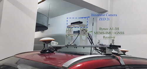
Field experiments are conducted to evaluate the performance of our methods. Figure 6 shows our platform equipped with a Bynav MEMS-IMU/GNSS integrated system and a ZED binocular camera. The gyroscope drift error of the MEMS-IMU is 2.7°/s with a random walk error of 1°/√hr. The accelerometer drift error is 3 mg with a random walk error of 300 µg/√Hz. GNSS runs at 1 Hz, the camera runs at 30 Hz@1080p and the MEMS-IMU runs at 100 Hz. The output frequency of our solution is in accordance with that of GNSS as 1 Hz. The camera and the integrated system are spatiotemporal synchronized.

Figure 6. Our experimental platform which consists of a binocular camera and a GNSS/MEMS-IMU integrated system.

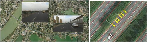
To completely evaluate our methods, our platform first ran on an urban expressway in Wuhan, China, as shown in Figure 7. The testing travel lasted about 15 minutes with an average speed of 50 km/h. In addition, another GNSS receiver (Septentrio PolaRx5) with precisely known coordinates is set up as a reference station and the baseline is within 5 km. The ground truth of the vehicle position, velocity and attitude is generated by the post-processing kinematic (PPK)/INS integration through commercial software Inertial Explorer, using the dual-frequency GNSS measurements and MEMS-IMU measurements. The overall positioning accuracy is at centimeter-level and the fixed rate is 97.3%, which can facilitate a fair and reliable performance comparison between different algorithms in the following evaluation.

Figure 7. Testing trajectory (left) and a part of the prior map in lanelets format (right). Red discrete points represent lane boundaries and yellow arrows point to SE points.

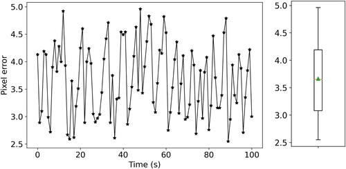
Figure 8 shows the visual lane line detection result. Line segments that locate on the left side and near the bottom of the image are chosen as our target line segment. Averaged values of the upper two ends of the target line segment in the image are extracted as the target SE. In (12), we need to estimate the accuracy of measured row coordinates $u$ of SEs, which means how many pixel difference between the measured row coordinate and the actual row coordinate. The true coordinates of SEs in the e-frame from the map are transformed to the c-frame according to camera calibration extrinsic parameters and ground truth of vehicle trajectory. Then the actual row coordinates of SEs are calculated by (6). Figure 9 shows the pixel errors of our method. We can see that the pixel errors fluctuate randomly between 2.5 and 5. The randomness is caused by various lighting conditions, road conditions and the qualities of lane lines in the images. We use the mean pixel error 3.66 as ${\delta }_u$ in (12).

Figure 8. Visual detection results of lane lines and lane corners for the left camera.

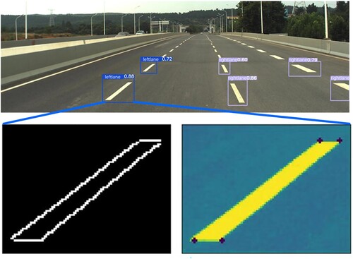
Figure 9. Left plot shows pixel errors of visual SE detection, and the right plot shows the boxplot of pixel errors from all time steps, where orange line represents median value and green triangle represents mean value.

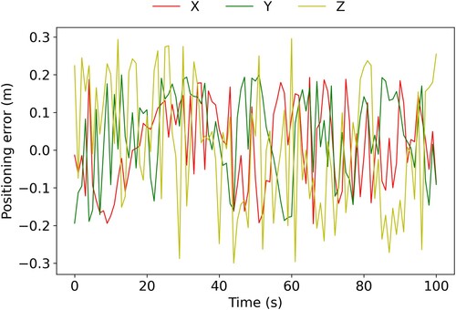
To demonstrate the positioning effect of our vision-based relative positioning approach more intuitively, positioning errors in the c-frame corresponding to Figure 9 are shown in Figure 10. We can see that our method can achieve an accuracy of less than 0.3 m, which can provide a strong constraint in AR. The positioning error in Z-direction is larger than that in X- and Y-directions, which is also consistent with the principle of binocular stereo positioning.

Figure 10. Positioning errors of our vision-based relative positioning method in the X-, Y- and Z-directions in the c-frame.

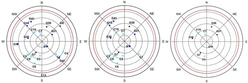
To better evaluate our methods, we first simulate three GNSS observation conditions with elevation cutoff angle 10°, 30° and 50°, in which 10° and 30° correspond to urban environments and 50° corresponds to high occlusion environment. Figure 11 shows the sky plot of visible satellites of GPS + BDS above the platform’s horizon at the first epoch for the three observation conditions. There are much more visible satellites in the simulated urban environments (10° and 30°) than those in the simulated high occlusion environment (50°).

Figure 11. Sky plot of visible satellites of GPS + BDS above the platform’s horizon at the first epoch. Left: simulated urban environment with cutoff angle 10°, middle: simulated urban environment with cutoff angle 30°, right: simulated urban environment with cutoff angle 50°. GPS satellites are represented by blue dots and their numbers starts with a letter ‘G.’ BDS satellites are represented by cyan dots and their numbers starts with a letter ‘C’.

Figure 12 shows the time series of positioning errors of GNSS RTK results in the three environments. We can see that GNSS RTK can achieve meter-level positioning results in the simulated urban environments. However, the positioning accuracy in the simulated high occlusion environment is much worse when more satellites are excluded. To evaluate the AR performance, here we use fixed rate and success rate as evaluation criteria, which are calculated as (14) $\begin{array}{rl}& \mathrm{fixed}\mathrm{rate}={\displaystyle \frac{\mathrm{Number}\mathrm{of}\mathrm{fixed}\mathrm{epochs}}{\mathrm{Total}\mathrm{Number}\mathrm{of}\mathrm{epochs}}}\\ & \mathrm{success}\mathrm{rate}={\displaystyle \frac{\mathrm{Number}\mathrm{of}\mathrm{correctly}\mathrm{fixed}\mathrm{epochs}}{\mathrm{Total}\mathrm{Number}\mathrm{of}\mathrm{epochs}}}\end{array}$(14) For each epoch, if the ratio value from AR is larger than 3, we assume the epoch is fixed. If the position solution $p(x,y,x)$ of AR and the position ground truth $\mathrm{GT}(G{T}_x,G{T}_y,G{T}_z)$ meet the requirement: (15) $|x-G{T}_x|<0.05m\mathrm{and}|y-G{T}_y|<0.05m\mathrm{and}|z-G{T}_z|<0.1m$(15) we assume the epoch is correctly fixed.

Figure 12. Positioning errors of GNSS RTK in northern, eastern and up directions for the three simulated environments: cutoff angle 10° (left), cutoff angle 30° (middle) and cutoff angle 50° (right).

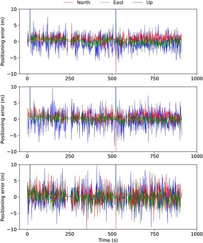
Table 1 illustrates the RMSE values, fixed rates and success rates in the three environments. Even though there are enough number of visible satellites in the simulated urban environments, their fixed rates and success rates are low, this is due to the noises in the pseudorange measurements, which may be caused by sound barriers on expressways in Figure 7 (left).

Table 1. Positioning errors, fixed rates and success rates of GNSS RTK for the three simulated environments.

Cutoff angle	RMSE (m)			Fixed rate (%)	Success rate (%)
	North	East	Up
10°	1.39	1.12	2.42	7.1%	6.7%
30°	1.49	1.12	2.68	9.3%	8.5%
50°	2.30	1.99	3.0	16.4%	0.0%

To comprehensively evaluate the performance of our method (GNSS/Vision/INS/Map, GVIM), it is compared with a GNSS/INS tightly coupled integration system (GINS) and a well-known tightly coupled GNSS-Visual-Inertial fusion system (GVINS) (Cao, Lu, and Shen 2022). Note that GVINS tightly couples GNSS raw pseudorange measurements and Doppler measurements with inertial and visual measurements, therefore it does not have phase ambiguities and AR, and we use it to evaluate the positioning performance of method. GINS uses GNSS raw pseudorange measurements and carrier phase measurements in the tightly integrated system, so we use it to evaluate both positioning performance and AR performance of our method.

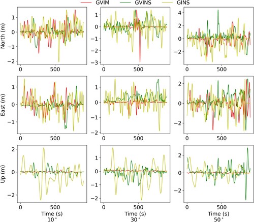
Figure 13 shows that when cutoff angle is 10°, all GVIM, GINS and GVINS can reach a submeter-level accuracy with a few meter-level outliers, and our method GVIM provides the lowest positioning errors in all directions. When cutoff angle is set to 30° or 50°, the positioning errors increase to meter level while our method still keeps the best positioning performance. In all the three environments, GINS performs worse in up directions with large fluctuations, while GVINS and GVIM constrain the positioning errors by introducing visual measurements, especially our method GVIM keeps high precision in up direction. This is because the high-precision elevation information of SEs from the map imposes strong elevation constraints on the vehicle.

Figure 13. Positioning errors of GVIM, GINS and GVINS in northern, eastern and up directions for the three simulated environments: cutoff angle 10° (left), cutoff angle 30° (middle) and cutoff angle 50° (right).

Table 2 illustrates their RMSE values, fixed rates and success rates. We can see that our method performs the best, with an improvement of (5.1%, 54.3%, 83%) in terms of 3D positioning accuracy with respect to GVINS, GINS and RTK, respectively, in the simulated urban environment with cutoff angle 10°, with an improvement of (44.6%, 65.6%, 88.3%) in the simulated urban environment with cutoff angle 30°, and with an improvement of (26.8%, 39.4%, 76.1%) in the simulated high occlusion environment with cutoff angle 50°. The ambiguity -fixed rate increases (26%, 29.2%) and the success rate increases (27.5%, 28.3%) with respect to GINS and RTK, respectively, in the simulated urban environment with cutoff angle 10°, the ambiguity-fixed rate increases (59.6%, 63.9%) and the success rate increases (61.7%, 62.3%) in the simulated urban environment with cutoff angle 30°, and the ambiguity-fixed rate increases (13.6%, 17%) and the success rate increases (23.4%, 23.4%) in the simulated high occlusion environment with cutoff angle 50°. The results from GVIM also demonstrate that accurate elevation constraints can lead to centimeter-level position in up direction.

Table 2. Positioning errors and fixed rates of four methods in the three simulated environments.

Cutoff angle	Methods	RMSE (m)				Fixed rate (%)	Success rate (%)
		North	East	Up	3D
10°	GVIM	0.37	0.35	0.04	0.51	36.3%	35%
	GVINS	0.33	0.32	0.28	0.54	/	/
	GINS	0.52	0.49	0.86	1.12	10.3%	7.5%
	GNSS RTK	1.39	1.12	2.42	3.0	7.1%	6.7%
30°	GVIM	0.33	0.19	0.04	0.38	73.2%	70.8%
	GVINS	0.42	0.43	0.34	0.69	/	/
	GINS	0.65	0.52	0.74	1.11	13.6%	9.1%
	GNSS RTK	1.49	1.12	2.68	3.26	9.3%	8.5%
50°	GVIM	0.70	0.74	0.03	1.02	33.4%	23.4%
	GVINS	0.90	0.80	0.70	1.39	/	/
	GINS	1.28	0.86	0.67	1.68	19.8%	0%
	GNSS RTK	2.30	1.99	3.0	4.27	16.4%	0%

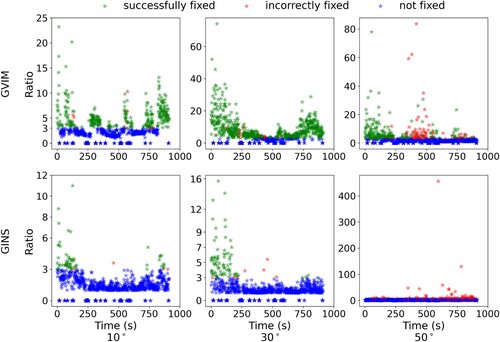
To further analyze the AR performance between our method GVIM and GINS, Figure 14 shows times series of ratio values from the LAMBDA method in the two methods. If ratio is larger than 3, we assume its corresponding phase ambiguity is fixed. The calculated phase ambiguities are compared with their ground truths to judge if they are fixed successfully. From Figure 14, we can see that GVINS fails at fixing ambiguities or fixing ambiguities incorrectly at most epochs, especially in the simulated high occlusion environment with cutoff angle 50°. Our method GVIM performs the best in the simulated urban environment with cutoff angle 30° with a success rate of 70.8%. It maybe because that the cutoff angle 30° eliminates noisy pseudorange measurements of low satellites, which may be caused by sound barriers on expressways in Figure 7 (left), and it also keeps enough available satellites for AR.

Figure 14. AR performances of our method GVIM (first row) and GVINS (second row) in simulated environments with cutoff angles 10° (first column), 30° (second column) and 50° (third column). Green and red stars mean phase ambiguities are fixed but red stars denote incorrect fixed ambiguities. Blue stars mean phase ambiguities are not fixed.

Figure 15 shows the time series of yaw angle errors in the three simulated environments. GINS performs the worst among the three methods and shows a large drift over time in scenarios with cutoff angle 10° and 50°. GVINS also shows a drift over time in these two scenarios, but slower than GINS, and its yaw angle error fluctuates frequently in the 50° scenario, which maybe because the large positioning errors affect the yaw estimation. Our method GVIM performs much better than GVINS and GINS in scenarios with cutoff angle 10° and 30°, but it also shows a drift over time in the 50° scenario, which maybe also resulting from large positioning errors. Table 3 shows the statistic results of the yaw angle errors of the three methods in the simulated environments. We can see that GVIM can achieve sub-degree level yaw angle error in the simulated urban environments, with an improvement (48.9%, 59.1%) respect to GVINS and GINS in the 10° scenario, and with an improvement (77.1%, 91.6%) in the 30° scenario.

Figure 15. Yaw angle errors of GVIM, GINS and GVINS in the three simulated environments: cutoff angle 10° (left), cutoff angle 30° (middle) and cutoff angle 50° (right).

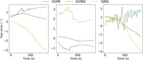
Table 3. RMSE of yaw angle errors of GVIM, GINS and GVINS in the three simulated environments.

Cutoff angle	Yaw angle RMSE (°)
	GVIM	GVINS	GINS
10°	0.65	1.27	1.59
30°	0.19	0.83	2.27
50°	1.27	1.19	1.34

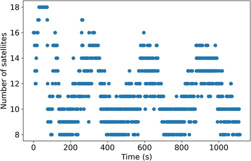
To verify our method in real dense urban area, we collect data using the platform around a playground in our campus in Wuhan, as shown in Figure 16. The ground truth of the vehicle position, velocity and attitude is achieved as the same as the above simulated experiment. The overall positioning accuracy is at centimeter level and the fixed rate is more than 90%. Figure 17 shows the number of visible GPS + BDS satellites during observation. We can see that the average number is only 10.44 caused by dense forest canopies and high buildings, which gives rise to severe signal blockages and multipaths. The satellite number shows three repeated patterns, which is due to our platform circling the playground three times.

Figure 16. Overview of the testing trajectory and urban scenarios in GNSS partly-blocked conditions.

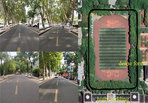
Figure 17. Number of visible GPS + BDS satellites during observation.

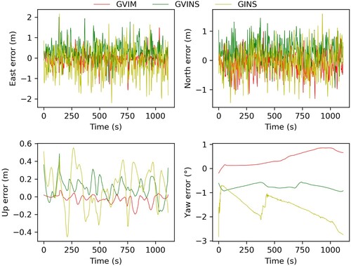
Figure 18 shows the positioning errors and yaw estimation errors of our method GVIM, GINS and GVINS. All the three methods can achieve submeter-level positioning accuracy in most epochs, including GINS due to its tightly coupling strategy. Compared with the positioning results of the simulated experiments in Figure 13, the three methods show similar performances. GVIM and GVINS outperform GINS as they introduce visual measurements to constrain positioning errors, and GVIM performs the best especially in the up direction due to the high-precision elevation constraint of SEs from the map. Regarding to yaw angle estimation, similar to Figure 15, the three methods also show slight drifts over time, and the error of GVIM is closer to 0 than GVINS and GINS.

Figure 18. Positioning errors of GVIM, GVINS and GINS in northern, eastern and up directions and yaw estimation errors in the real urban scenario.

Table 4 illustrates the RMSE values, fixed rates and success rates of GVIM, GVINS, GINS and RTK. We can see that our method GVIM preforms the best, with an improvement of (42.3%, 10%, 64.3%) in terms of northern, eastern and up positioning accuracy with respect to GVINS, with an improvement of (53.1%, 20%, 78.3%) with respect to GINS, and with an improvement of (70.6%, 53.8%, 96.1%) with respect to RTK. The ambiguity-fixed rate increases (71.7%, 87.7%) and the success rate increases (80.1%, 92.4%) with respect to GINS and RTK respectively. The yaw angle estimation accuracy increases (32.9%, 69.5%) with respect to GVINS and GINS respectively.

Table 4. Positioning RMSE, yaw estimation RMSE, fixed rates and success rate of four methods in the real urban scenario.

Methods	RMSE (m)				RMSE (°)	Fixed rate (%)	Success rate (%)
	North	East	Up	3D	Yaw
GVIM	0.30	0.36	0.05	0.45	0.51	59.4%	55.4%
GVINS	0.52	0.40	0.14	0.56	0.76	/	/
GINS	0.64	0.45	0.23	0.78	1.67	16.8%	11%
GNSS RTK	1.02	0.78	1.27	1.81	/	7.3%	4.2%

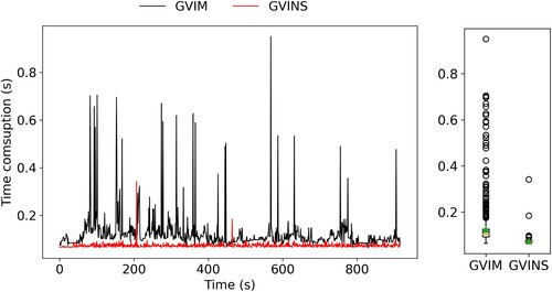
In addition to the positioning accuracy and AR performance comparisons, we also analyze the real-time performance of the proposed method, which is essential for intelligent vehicle operating in cities. The experimental data is processed on the platform with an Intel Core i7-7500U CPU at 2.7 GHz and 8GB of RAM. Since GINS does not need to process image and map data, the time consumed for each epoch is only a few milliseconds, so we compare the processing time between GVIM and GVINS. Figure 19 shows the time consumption for each epoch of our method and GVINS in the simulated urban environment with cutoff angle 10°. We can see that GVIM owns the median and mean time consumptions of 104 and 120 ms respectively, and those of GVINS are 72 and 74 ms respectively. As GVIM involves visual lane extraction and map matching, it is less efficient than GVINS. In our work, the map data is organized with R-tree, but a more efficient map organization (e.g. graph) should further improve the computational efficiency of GVIM.

Figure 19. Time consumption of our method GVIM and GVINS in the simulated environment with cutoff angle 10°. The left plot shows time consumption per time step, and the right plot shows the boxplot of time consumptions from all time steps, where orange line represents median value and green triangle represents mean value.

8. Conclusion and discussion

In this work, we propose a vision-aided single-epoch AR by tightly coupling raw measurements from GNSS, INS, camera and map information. At each epoch, a map-based positioning by ambiguous lane matching is proposed to find all possible rectangles where the vehicle may locate, considering the repeatability of lane lines. A vision-based relative positioning is then applied by measuring the relative position between the lane line corner and the vehicle. Finally, the two positioning results are introduced into GNSS RTK single-epoch AR to find the most accurate ambiguity estimations and position and yaw angle estimations. The vehicular experiments in simulated and real GNSS partly-blocked conditions were conducted to evaluate the effectiveness of the proposed method. Experimental results prove that our method performs much better than GVINS and GINS in terms of both position and yaw angle.

On the one hand, the detection accuracy of visual lane line end point is 3.66 pixels in our experiments, which needs to be further improved in the future. A sub-pixel level detection accuracy can significantly improve the relative positioning precision. On the other hand, our method is less efficient than GVINS and GINS in terms of time consumption as it involves image processing and map matching. In future work, we will focus on developing better map organization to speed up map matching and establishing a more efficient visual lane extraction algorithm.

Author contributions

HZ, CQ, WL, and BL contributed to the conception of the study. HZ and CQ and WL collected, analyzed the data and verified the results. HZ wrote the main manuscript text. HZ provided funding. All authors reviewed the manuscript.

Disclosure statement

No potential conflict of interest was reported by the author(s).

Data availability statement

The data can be made available upon request by contacting the authors.

Additional information

Funding

This research gets support from the National Key R&D Program of China (Grant No. 2023YFB3907102) and the National Natural Science Foundation of China (Grant No. 52332010).

References

- Bender, Philipp, Julius Ziegler, and Christoph Stiller. 2014. “Lanelets: Efficient Map Representation for Autonomous Driving.” 2014 IEEE Intelligent Vehicles Symposium Proceedings, 420–425. https://doi.org/10.1109/IVS.2014.6856487.
- Blewitt, Geoffrey. 1990. “An Automatic Editing Algorithm for GPS Data.” Geophysical Research Letters 17 (3): 199–202. https://doi.org/10.1029/GL017i003p00199.
- Cao, Shaozu, Xiuyuan Lu, and Shaojie Shen. 2022. “GVINS: Tightly Coupled GNSS–Visual–Inertial Fusion for Smooth and Consistent State Estimation.” IEEE Transactions on Robotics 38 (4): 2004–2021. https://doi.org/10.1109/TRO.2021.3133730.
- Carcanague, Sébastien. 2012. “Real-time Geometry-Based Cycle Slip Resolution Technique for Single-Frequency PPP and RTK.” Proceedings of the 25th International Technical Meeting of The Satellite Division of the Institute of Navigation (ION GNSS 2012), 1136–1148.
- de Lacy, Maria Clara, Mirko Reguzzoni, and Fernando Sansò. 2012. “Real-time Cycle Slip Detection in Triple-Frequency GNSS.” GPS Solutions 16 (3): 353–362. https://doi.org/10.1007/s10291-011-0237-5.
- Deng, Chenlong, Qian Liu, Xuan Zou, Weiming Tang, Jianhui Cui, Yawei Wang, and Chi Guo. 2020. “Investigation of Tightly Combined Single-Frequency and Single-Epoch Precise Positioning Using Multi-GNSS Data.” Remote Sensing 12 (2): 285. https://doi.org/10.3390/rs12020285.
- El-Sheimy, Naser. 2004. “Inertial Techniques and INS/DGPS Integration.” Engo 623-Course Notes:170-182.
- El-Sheimy, Naser, and Ahmed Youssef. 2020. “Inertial Sensors Technologies for Navigation Applications: State of the art and Future Trends.” Satellite Navigation 1 (1): 2. https://doi.org/10.1186/s43020-019-0001-5.
- Gao, Zhouzheng, Maorong Ge, Wenbin Shen, Hongping Zhang, and Xiaoji Niu. 2017. “Ionospheric and Receiver DCB-Constrained Multi-GNSS Single-Frequency PPP Integrated with MEMS Inertial Measurements.” Journal of Geodesy 91 (11): 1351–1366. https://doi.org/10.1007/s00190-017-1029-7.
- Gong, Zheng, Peilin Liu, Fei Wen, Rendong Ying, Xingwu Ji, Ruihang Miao, and Wuyang Xue. 2020. “Graph-Based Adaptive Fusion of GNSS and VIO Under Intermittent GNSS-Degraded Environment.” IEEE Transactions on Instrumentation and Measurement 70:1–16. https://doi.org/10.1109/tim.2020.3039640.
- He, Haibo, Jinlong Li, Yuanxi Yang, Junyi Xu, Hairong Guo, and Aibing Wang. 2014. “Performance Assessment of Single-and Dual-Frequency BeiDou/GPS Single-Epoch Kinematic Positioning.” GPS Solutions 18 (3): 393–403. https://doi.org/10.1007/s10291-013-0339-3.
- Kasmi, Abderrahim, Johann Laconte, Romuald Aufrère, Dieumet Denis, and Roland Chapuis. 2020. “End-to-end Probabilistic Ego-Vehicle Localization Framework.” IEEE Transactions on Intelligent Vehicles 6 (1): 146–158. https://doi.org/10.1109/TIV.2020.3017256.
- Li, Xingxing, Shengyu Li, Yuxuan Zhou, Zhiheng Shen, Xuanbin Wang, Xin Li, and Weisong Wen. 2022. “Continuous and Precise Positioning in Urban Environments by Tightly Coupled Integration of GNSS, INS and Vision.” IEEE Robotics and Automation Letters 7 (4): 11458–11465. https://doi.org/10.1109/LRA.2022.3201694.
- Li, Bofeng, Yanan Qin, Zhen Li, and Lizhi Lou. 2016. “Undifferenced Cycle Slip Estimation of Triple-Frequency BeiDou Signals with Ionosphere Prediction.” Marine Geodesy 39 (5): 348–365. https://doi.org/10.1080/01490419.2016.1207729.
- Li, Bofeng, Yanan Qin, and Tianxia Liu. 2019. “Geometry-Based Cycle Slip and Data gap Repair for Multi-GNSS and Multi-Frequency Observations.” Journal of Geodesy 93 (3): 399–417. https://doi.org/10.1007/s00190-018-1168-5.
- Li, Xingxing, Xuanbin Wang, Jianchi Liao, Xin Li, Shengyu Li, and Hongbo Lyu. 2021. “Semi-Tightly Coupled Integration of Multi-GNSS PPP and S-VINS for Precise Positioning in GNSS-Challenged Environments.” Satellite Navigation 2 (1): 1–14. https://doi.org/10.1186/s43020-020-00033-9.
- Li, Tuan, Hongping Zhang, Zhouzheng Gao, Qijin Chen, and Xiaoji Niu. 2018. “High-Accuracy Positioning in Urban Environments Using Single-Frequency Multi-GNSS RTK/MEMS-IMU Integration.” Remote Sensing 10 (2): 205. https://doi.org/10.3390/rs10020205.
- Li, Tuan, Hongping Zhang, Xiaoji Niu, and Zhouzheng Gao. 2017. “Tightly-Coupled Integration of Multi-GNSS Single-Frequency RTK and MEMS-IMU for Enhanced Positioning Performance.” Sensors 17 (11): 2462. https://doi.org/10.3390/s17112462.
- Li, Qingquan, Jian Zhou, Bijun Li, Yuan Guo, and Jinsheng Xiao. 2018. “Robust Lane-Detection Method for low-Speed Environments.” Sensors 18 (12): 4274. https://doi.org/10.3390/s18124274.
- Liu, Fei. 2018. Tightly Coupled Integration of GNSS/INS/Stereo Vision/Map Matching System for Land Vehicle Navigation. University of Calgary. https://doi.org/10.11575/PRISM/31740
- Lu, Yan, Jiawei Huang, Yi-Ting Chen, and Bernd Heisele. 2017. “Monocular Localization in Urban Environments Using Road Markings.” 2017 IEEE Intelligent Vehicles Symposium (IV), 468–474. https://doi.org/10.1109/ivs.2017.7995762.
- Niu, Xiaoji, Hailiang Tang, Tisheng Zhang, Jing Fan, and Jingnan Liu. 2022. “IC-GVINS: A Robust, Real-Time, INS-Centric GNSS-Visual-Inertial Navigation System.” IEEE Robotics and Automation Letters 8 (1): 216–223. https://doi.org/10.1109/lra.2022.3224367.
- Odolinski, Robert, and Peter JG Teunissen. 2016. “Single-frequency, Dual-GNSS Versus Dual-Frequency, Single-GNSS: A low-Cost and High-Grade Receivers GPS-BDS RTK Analysis.” Journal of Geodesy 90 (11): 1255–1278. https://doi.org/10.1007/s00190-016-0921-x.
- Pöppl, Florian, Hans Neuner, Gottfried Mandlburger, and Norbert Pfeifer. 2023. “Integrated Trajectory Estimation for 3D Kinematic Mapping with GNSS, INS and Imaging Sensors: A Framework and Review.” ISPRS Journal of Photogrammetry and Remote Sensing 196:287–305. https://doi.org/10.1016/j.isprsjprs.2022.12.022.
- Psychas, Dimitrios, Sandra Verhagen, and Peter JG Teunissen. 2020. “Precision Analysis of Partial Ambiguity Resolution-Enabled PPP Using Multi-GNSS and Multi-Frequency Signals.” Advances in Space Research 66 (9): 2075–2093. https://doi.org/10.1016/j.asr.2020.08.010.
- Qin, Tong, Yuxin Zheng, Tongqing Chen, Yilun Chen, and Qing Su. 2021. “A Light-Weight Semantic map for Visual Localization Towards Autonomous Driving.” 2021 IEEE International Conference on Robotics and Automation (ICRA), https://doi.org/10.1109/icra48506.2021.9561663.
- Rabe, Johannes, Martin Hübner, Marc Necker, and Christoph Stiller. 2017. “Ego-lane Estimation for Downtown Lane-Level Navigation.” 2017 IEEE Intelligent Vehicles Symposium (IV), https://doi.org/10.1109/ivs.2017.7995868.
- Rabe, Johannes, Marc Necker, and Christoph Stiller. 2016. “Ego-lane Estimation for Lane-Level Navigation in Urban Scenarios.” 2016 IEEE Intelligent Vehicles Symposium (IV), https://doi.org/10.1109/ivs.2016.7535494.
- Saudi, Azali, Jason Teo, Mohd Hanafi Ahmad Hijazi, and Jumat Sulaiman. 2008. “Fast Lane Detection with Randomized Hough Transform.” 2008 International Symposium on Information Technology. https://doi.org/10.1109/itsim.2008.4631879.
- Schreiber, Markus, Carsten Knöppel, and Uwe Franke. 2013. “Laneloc: Lane Marking Based Localization Using Highly Accurate Maps.” Paper presented at the 2013 IEEE Intelligent Vehicles Symposium (IV), https://doi.org/10.1109/ivs.2013.6629509.
- Shunsuke, Kamijo, Gu Yanlei, and Li-Ta Hsu. 2015. “GNSS/INS/on-Board Camera Integration for Vehicle Self-Localization in Urban Canyon.” 2015 IEEE 18th International Conference on Intelligent Transportation Systems, https://doi.org/10.1109/itsc.2015.407.
- Suhr, Jae Kyu, Jeungin Jang, Daehong Min, and Ho Gi Jung. 2016. “Sensor Fusion-Based low-Cost Vehicle Localization System for Complex Urban Environments.” IEEE Transactions on Intelligent Transportation Systems 18 (5): 1078–1086. https://doi.org/10.1109/TITS.2016.2595618.
- Tao, Zui, Philippe Bonnifait, Vincent Frémont, Javier Ibanez-Guzman, and Stéphane Bonnet. 2017. “Road-Centered Map-Aided Localization for Driverless Cars Using Single-Frequency GNSS Receivers.” Journal of Field Robotics 34 (5): 1010–1033. https://doi.org/10.1002/rob.21708.
- Teunissen, P. J. G., P. J. De Jonge, and C. C. J. M. Tiberius. 1995. “The LAMBDA Method for Fast GPS Surveying.” International Symposium “GPS Technology Applications”. Bucharest, Romania.
- Wen, Weisong, Xiwei Bai, Guohao Zhang, Shengdong Chen, Feng Yuan, and Li-Ta Hsu. 2020. “Multi-Agent Collaborative GNSS/Camera/INS Integration Aided by Inter-Ranging for Vehicular Navigation in Urban Areas.” IEEE Access 8:124323–124338. https://doi.org/10.1109/ACCESS.2020.3006210.
- Xiao, Zhongyang, Kun Jiang, Shichao Xie, Tuopu Wen, Chunlei Yu, and Diange Yang. 2018. “Monocular Vehicle Self-Localization Method Based on Compact Semantic map.” 2018 21st International Conference on Intelligent Transportation Systems (ITSC), 3083–3090. https://doi.org/10.1109/ITSC.2018.8569274.
- Xiao, Zhongyang, Diange Yang, Tuopu Wen, Kun Jiang, and Ruidong Yan. 2020. “Monocular Localization with Vector HD map (MLVHM): A Low-Cost Method for Commercial IVs.” Sensors 20 (7): 1870. https://doi.org/10.3390/s20071870.
- Yan, Wenlin, Luísa Bastos, José A Gonçalves, Américo Magalhães, and Tianhe Xu. 2018. “Image-aided Platform Orientation Determination with a GNSS/low-Cost IMU System Using Robust-Adaptive Kalman Filter.” GPS Solutions 22 (1): 12. https://doi.org/10.1007/s10291-017-0676-8.
- Zhang, Zhen, Xiao Ai, and Naim Dahnoun. 2013. “Efficient Disparity Calculation Based on Stereo Vision with Ground Obstacle Assumption.” 21st European Signal Processing Conference (EUSIPCO 2013), 1–5.
- Zhang, Xiaohong, and Xiyang He. 2016. “Performance Analysis of Triple-Frequency Ambiguity Resolution with BeiDou Observations.” GPS Solutions 20 (2): 269–281. https://doi.org/10.1007/s10291-014-0434-0.
- Zhang, Xiaohong, Feng Zhu, Yuxi Zhang, Freeshah Mohamed, and Wuxing Zhou. 2019. “The Improvement in Integer Ambiguity Resolution with INS Aiding for Kinematic Precise Point Positioning.” Journal of Geodesy 93 (7): 993–1010. https://doi.org/10.1007/s00190-018-1222-3.
- Zhu, Sh, S. H. Li, Y. Liu, and Q. W. Fu. 2019. “Low-Cost MEMS-IMU/RTK Tightly Coupled Vehicle Navigation System with Robust Lane-Level Position Accuracy.” 2019 26th Saint Petersburg International Conference on Integrated Navigation Systems (ICINS). 1–4. https://doi.org/10.23919/icins.2019.8769351.