Sea-level monitoring in the British Overseas Territories

Abstract

A review is conducted on the status of sea-level monitoring in the British Overseas Territories (BOTs), showing where measurements have been made in the last two decades by various groups and thereby indicating where investments in future recording are needed. The sea level has risen in every territory since the early 1990s, and is predicted to increase by approximately 0.25–1.0 m by the end of the twenty-first century, depending on the emissions scenario. As a result, it is maintained that sea-level monitoring is needed in all BOTs, both for local coastal applications and as British contributions to the worldwide sea-level monitoring programme.

Introduction

This article is concerned with sea-level monitoring in the British Overseas Territories (BOTs). These are the 14 remaining parts of the former British empire that once covered a quarter of the globe (Cannon 2009; Wikipedia 2014). Most of the territories are small islands in the North and South Atlantic, with more distant outposts in the Indian and Pacific Oceans and Antarctica (Table 1 and Figure 1).

Figure 1. Map of the locations of the British Overseas Territories in Table 1 (red dots) and two additional stations (blue dots).

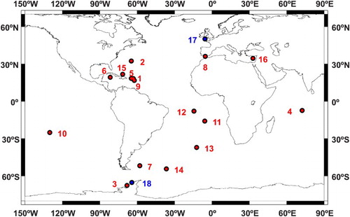
Table 1. The BOT locations shown in Figure 1, giving the main or nearest tide gauge, as represented in the PSMSL database, together with the authority responsible for operating the gauge.

Station number in Figure 1	British Overseas Territory	Nearest tide gauge^a	Location^b	Operator
1	Anguilla	Lime Tree Bay, St Croix, US Virgin Islands	N (200 km)	NOAA
2	Bermuda	Bermuda, St George's	B	NOAA
3	British Antarctic Territory	Rothera	B	NOC/BAS
4	British Indian Ocean Territory	Diego Garcia	B	UHSLC
5	British Virgin Islands	Charlotte Amalie, US Virgin Islands	N (30 km)	NOAA
6	Cayman Islands	Casilda, Cuba	N (300 km)	CNTS
7	Falkland Islands	Stanley	B	NOC
8	Gibraltar	Gibraltar	B	NOC
9	Montserrat	Guadaloupe	N (100 km)	Météo-France
10	Pitcairn Group of Islands	Rikitea, French Polynesia	N (700 km)	UHSLC/SHOM
11	St Helena, Ascension and Tristan da Cunha	St Helena	B	NOC
12	St Helena, Ascension and Tristan da Cunha	Ascension	B	NOC
13	St Helena, Ascension and Tristan da Cunha	Tristan da Cunha	B	NOC
14	South Georgia and the South Sandwich Islands	King Edward Point, South Georgia	B	NOC/BAS
15	Turks and Caicos Islands	Gibara, Cuba	N (450 km)	CNTS
16	Sovereign Bases Areas on Cyprus (Akrotiri and Dhelalia)	Hadera, Israel	N (300 km)	IOLR
	Additional Tide Gauges
17	UK	Newlyn	UK	NOC/EA
18	British Antarctic Territory	Vernadsky/Faraday	B	NOC/NASC

Note: ^aThe ‘nearest tide gauge’ is the nearest gauge having an extended record in the PSMSL; ^bB = gauge is located in the British Overseas Territory, N = gauge is in a neighbouring country at the approximate distance stated. BAS = British Antarctic Survey (UK); CNTS = Cuban National Tidal Service; EA = Environment Agency (UK); IOLR = Israel Oceanographic and Limnological Research; NASC = National Antarctic Scientific Center (Ukraine); NOAA = National Oceanic and Atmospheric Administration (US); NOC = National Oceanography Centre (UK); SHOM = Service Hydrographique et Océanographique de la Marine (France); UHSLC = University of Hawaii Sea Level Center (US).

The BOTs present a fascinating selection of different coastal types. Thanks to their geographical spread and relative isolation, they together have more biodiversity than the United Kingdom (UK) itself. Some of them are United Nations Educational, Scientific and Cultural Organization (UNESCO) World Heritage Sites. All coastal communities, including those of the BOTs, have a practical need for access to sea-level data from modern tide gauges. These data provide engineers with the information on extreme sea levels that they need for designing robust coastal defences, and infrastructure such as quaysides and promenades. Environmentalists also need to know the frequency and magnitude of high sea levels during storms that result in beach erosion and the flooding of sensitive natural habitats. Everyone with an interest in the coast needs access to the best possible advice from sea-level scientists as to the likely magnitudes and rates of change of sea level in the future.

Long-term sea-level rise represents a threat to many sections of BOT coastlines, including the sandy beaches of the Caribbean (used by both turtles and tourists), the corals of the Chagos Archipelago (British Indian Ocean Territory), and the coastal infrastructure of harbours such as at Gibraltar, Stanley (the Falkland Islands) and St Helena. The understanding of sea-level change and its impacts, within the overall context of climate change, has recently been reviewed by the Intergovernmental Panel on Climate Change (IPCC) Working Groups I and II (IPCC 2013, 2014a, 2014b). Chapters 3 and 13 in IPCC (2013) cover past and future sea-level change, while chapters 5 (coastal systems) and 29 (small islands) in IPCC (2014a, 2014b) are the most relevant regarding sea-level impacts at locations such as the BOTs.

Sea level monitoring in the BOTs

An understanding of sea-level change, and an appreciation of its impacts, will never be as complete as possible without having reliable data with which to confront the ocean and climate computer models upon which the IPCC depends. This implies having a means to monitor the sea level on a long-term basis.

Figure 1 shows that the BOTs (particularly the islands) provide ideal platforms for monitoring the sea level (and other physical, chemical and biological parameters) within vast ocean areas and so, if they were all instrumented with tide gauges and associated equipment, this would contribute significantly to the global sea-level monitoring objectives of the Global Sea Level Observing System (GLOSS) of the Intergovernmental Oceanographic Commission (IOC 2012). These worldwide in situ measurements of sea level would complement those provided on a quasi-global synoptic basis by satellite radar altimetry (Pugh & Woodworth 2014). The same equipment would provide all the sea-level data needed by engineers etc. for local purposes.

In fact, some BOTs have a long history of environmental monitoring (Kenworthy & Walker 1997), and sea level has been measured for different purposes. Short-term measurements, primarily for determining tidal characteristics, were made at many locations in the nineteenth century (Herschel 1849). The records of the Permanent Service for Mean Sea Level (PSMSL), the global data centre for long-term sea-level information, show that extended recordings of mean sea level (MSL) were made in Bermuda as early as 1833–1854, and in the Falklands in 1842 by the polar explorer James Clark Ross (Woodworth et al. 2010). Details of the availability of MSL information at each site can be obtained from the PSMSL website (http://www.psmsl.org).

However, in spite of the several good arguments for instrumenting all the territories, and although some have had a long history of sea-level recording, Table 1 shows that the current status of sea-level monitoring in the BOTs is not as complete as one might like. Of the sixteen BOT locations in Table 1, only seven have sea-level records provided by UK groups, while three others are provided via United States (US) agencies. The remaining six have no long records at all, and for these the nearest PSMSL long-term records in a neighbouring country are shown in Table 1. Some of these records are shown in Figure 2 in black (the Caribbean records are similar and are not all shown).

Figure 2. Records of monthly mean sea level (MSL) at each site from tide gauges (black) and altimetry (red) for sites in (a) the South Atlantic, (b) the North Atlantic and (c) other areas. Note: Tide-gauge names are shown in blue for sites in the BOTs themselves and black for sites in neighbouring countries (see Table 1). Some sites in the Caribbean in Table 1 are not included in these figures as their records are similar. For St Helena, Tristan and Diego Garcia, the separate sections of MSL data remain to be confirmed and are here estimated only. For some sites there are additional data available at the PSMSL subject to particular warning flags. Later data for all sites may be obtained from the centres shown in Table 2.

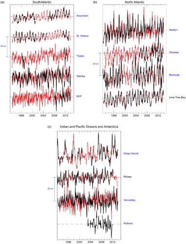
Table 1 and Figure 2 refer to two other locations. Newlyn is included in this paper as a representative of the 44-gauge network in the UK itself that is maintained by the National Oceanography Centre (NOC) on behalf of the Environment Agency. Vernadsky, a Ukrainian base on the west coast of the Antarctic Peninsula, was formerly a British Antarctic survey base called Faraday. That base has a venerable tide gauge that was originally installed as part of the International Geophysical Year in 1957/8. It is still in operation and provides the longest sea-level record in Antarctica. It is now maintained in a collaboration between the NOC and the National Antarctic Scientific Center of the Ukraine.

Figure 2 shows that some of the BOT tide-gauge records have large gaps, which are partly a consequence of the difficulty of access for maintenance visits (e.g., no airfields at some South Atlantic islands or at Pitcairn, or long flights by military aircraft for Diego Garcia), although at some locations maintenance is provided by excellent local contacts. The construction of a new airport at St Helena should help with access to the gauge there. However, in other BOTs there are only one or two non-ideal locations for a tide gauge, and even these are hard to maintain. For example, the only feasible location at Tristan da Cunha is in an enclosed small harbour exposed to harsh wave conditions, and tide gauges have tended not to operate there for long without damage. Moreover, those sections of the record that have been acquired successfully include large signals due to very local wave set-ups that have nothing to do with the sea level outside the harbour that needs to be measured.

Table 2 provides a list of data centres which hold tide-gauge information from the BOT locations in Table 1. The tide-gauge technology differs between agencies. For example, UK groups tend to use pressure and radar systems (Figure 3), while US groups have in the past mostly used acoustic systems (IOC 2006). In all cases, sea levels are recorded at ‘higher frequencies’ (typically averaged over 1, 6 or 15 minutes), with these values filtered to provide hourly values – which are optimal for most tidal and oceanographic studies – and then combined into monthly and annual means as archived by the PSMSL.

Figure 3. Examples of modern radar gauges at BOTs: (a) an OTT radar level sensor (RLS) at St Helena at the end of a cantilevered arm; (b) a Waterlog DAA 3611i gauge at Stanley on a shorter arm; and (c) an OTT Kalesto gauge installation at Gibraltar, in which the radar gauge transmits horizontally inside an aluminium tube, with the beam reflected off the 45 deg end of the tube (painted yellow on its outside) downwards to the sea surface.

Source: All photographs courtesy of the NOC.

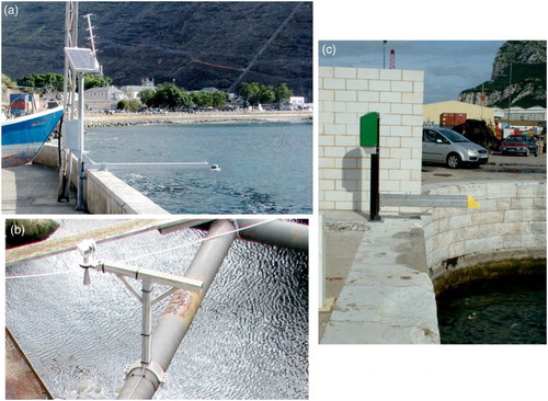
Table 2. Data centres holding tide-gauge data from BOT locations, types of data held and website names.

Tide-gauge data source	Data type	Website
NOC (South Atlantic, Antarctic and Gibraltar data)	Higher-frequency (e.g., 1- or 15-minute values) delayed-mode.	http://www.ntslf.org
NOC (UK data)	Higher-frequency (15-minute) delayed mode.	http://www.bodc.ac.uk
NOAA	Higher-frequency (6-minute) delayed mode.	http://tidesandcurrents.noaa.gov
UHSLC	Higher-frequency (mostly hourly) ‘research quality’ and ‘fast delivery’ delayed-mode.	http://uhslc.soest.hawaii.edu
PSMSL	Monthly and annual mean values.	http://www.psmsl.org
VLIZ	Higher-frequency (e.g., 1 minute) near real time.	http://www.ioc-sealevelmonitoring.org

Note: NOAA = National Oceanic and Atmospheric Administration (US); NOC = National Oceanography Centre (UK); PSMSL = Permanent Service for Mean Sea Level; UHSLC = University of Hawaii Sea Level Center (US); VLIZ = Flanders Marine Institute (Belgium).

Applications of tide-gauge data

As mentioned above, the arguments for providing sea-level monitoring at any coastal location, including those of the BOTs, are often constructed from one of two perspectives. One perspective involves ‘practical applications’, whereby continuous monitoring of levels is required for particular local purposes. The second perspective involves ‘scientific applications’ that have a local, regional or even global context, which complement the sea-level information provided by the irregular sampling of the global ocean by altimetry.

Many examples of both types of applications are available (IOC 2006; Pugh & Woodworth 2014), and these are summarized below. However, a point to stress is that one perspective need not exclude the other, and any proposal for funding for a new installation would be better constructed around both sets of applications. For example, inexpensive tide gauges are sometimes purchased by harbour authorities to provide an instantaneous display of the state of the tide, but the data are never shared and are anyway not of sufficient quality for other applications such as science. However, if there is already a good site for a tide gauge, then discussion with other sea-level stakeholders might result in a better-quality instrument being purchased, one which is capable of providing data for all applications, including science.

Practical applications

These applications include the use of tide-gauge data to determine ‘tidal constants’ from which predictions of high and low water levels and times can be computed. This sort of analysis has been undertaken for many years by the NOC, the UK Hydrographic Office, the National Oceanic and Atmospheric Administration (NOAA) and other groups. Such tidal information is routinely published in diaries and newspapers, and can be accessed for many of the BOTS (see http://www.ntslf.org/tides). Tide tables are employed at many BOTS by port authorities, fishermen and other coastal users.

More sophisticated use of ‘delayed-mode’ tide-gauge data (i.e., data which have been subjected to quality control by a data centre and eventually made available to users) include the determination of statistics of non-tidal variability due to storm surges, and the calculation of extreme levels for flood-risk studies (e.g., the calculation of the ‘return periods’ at which particular levels may be exceeded). The latter are obviously of great importance to coastal engineers for the design of coastal defences and infrastructure. Local land survey data are often defined in terms of Mean Sea Level, which requires an extended period of measurement by a tide gauge, with MSL data transferred throughout a territory by geodetic methods.

One ‘real-time’ application of tide-gauge data is within storm-surge monitoring, either for instantaneous display of sea level or for onward transmission of the data to centres where surge levels are compared to those predicted by numerical models. Similarly, gauges can form an important component of a tsunami warning system. The Caribbean is often subject to tropical storms and hurricanes, and less often to tsunamis, and has recently benefited from investment in sensors for such real-time ‘multi-hazard’ sea-level monitoring (see http://www.ioc-tsunami.org). This includes at the Cayman and British Virgin Islands, where information from neighbouring countries is relied on (Table 1). Some of these data can be inspected in real time via the IOC Sea Level Monitoring Facility at the Flanders Marine Institute (http://www.ioc-sealevelmonitoring.org). Unfortunately, some of these instruments are simple pressure sensors which are subject to instrumental drift and so are not suitable for long-term mean sea-level studies.

Scientific applications

Data from the South Atlantic network have been used in many scientific studies of sea-level variability in a region of the southern hemisphere which has been under-sampled historically. Some examples at the high and low frequency ends of the variability spectrum include the impact of distant North Atlantic swell on Ascension and St Helena (Vassie et al. 2004), the identification of five-day waves in the atmosphere and ocean (Woodworth et al. 1995; Mathers & Woodworth 2004), and investigations of long-term sea-level trends at individual islands (Woodworth et al. 2005, 2010, 2012). Data from Stanley and the Antarctic bases have been used in several studies of coherence of sea level around Antarctica and changes in the transport of the Antarctic Circumpolar Current (ACC; Hughes et al. 2003; Meredith et al. 2004; Woodworth et al. 2006; Hibbert et al. 2010). The South Atlantic has also provided a test bed for the development of advanced tide-gauge technology (Woodworth et al. 1996). In the North Atlantic, data from Bermuda have been used in many studies of sea-level variations in the sub-tropical gyre and along the North American Atlantic coastline (Sturges & Hong 1995; Thompson & Mitchum 2014; Woodworth et al. 2014). Several papers have used Gibraltar and nearby Spanish and North African data in studies of exchange flows between the Atlantic and Mediterranean (Garrett et al. 1989). In the Indian Ocean, long-term changes in sea level in the Chagos Archipelago have been investigated using data from the tide gauge in Diego Garcia (Dunne et al. 2012). Altogether, these individual papers add up to a body of work that is comparable in size to that concerning sea-level variability in the UK itself.

These examples largely refer to studies at particular locations. However, the scientific value of sea-level data is most apparent when used in combination in a network (as for meteorological data). The GLOSS programme of the IOC is the mechanism by which international coordination takes place for network construction. Data from the tide gauges are then contributed to the PSMSL and other data centres, from which they are accessed by scientists for studies that eventually contribute to the IPCC scientific assessments. They also have a combined role in the validation of altimeter data (Mitchum 2000), which also eventually feeds into the IPCC. Data from tide gauges in the BOTs, made available via the PSMSL and other sea-level centres, contribute to many regional and global studies in this way.

Comparisons to satellite altimetry

For Figure 2 a period of approximately two decades starting in the early 1990s is used. This period saw the establishment of modern recording at BOTs in the South Atlantic and Antarctica, and coincided with what is sometimes called the ‘era of satellite altimetry’ that commenced with the launch of TOPEX/Poseidon in August 1992.

Figure 2 shows in red altimeter sea level obtained from the ‘reference series’ of the TOPEX/Poseidon, Jason-1 and Ocean Surface Topography Mission/Jason-2 missions spanning 1992 to 2013. (Rothera is not accompanied by an altimeter time series as its latitude is at the limit of the reference series and there is ice cover for half of the year. The altimeter data loss due to ice is less at Vernadsky.) The data are averaged within a ± 2 deg latitude/longitude box around each tide gauge and then filtered to provide a quasi-monthly sampling similar to that of the monthly MSL from the tide gauges, as archived by the PSMSL. In this case, a version of the reference series data set provided by Brian Beckley of the Goddard Space Flight Center is used, which is uncorrected for air pressure effects and so is more directly comparable to the sea levels measured by the tide gauges.

Altimetry cannot measure exactly at the coast, where the tide gauge is, due to the footprints of its radar and radiometer measurements overlapping with the land. Therefore, the magnitude of any correlation between the sea levels observed by the two methods depends on the variability in the open ocean being similar to that at the gauge itself (Vinogradov & Ponte 2011). This similarity does not apply to all locations or even all islands (Williams & Hughes 2013). However, for most of the BOTs, close agreement can be seen in Figure 2 between the two techniques in describing the variability of sea level on seasonal and interannual timescales. Small differences in the seasonal cycle observed by each technique are seen at Gibraltar, where the narrow strait means that the tide gauge and altimeter sample ocean areas with slightly different seasonal cycles (Menemenlis et al. 2007).

However, there are sometimes differences in the long-term trends measured by the two techniques. This is to be expected as there are differences between the types of sea level observed. Altimetry measures ‘geocentric sea level’, which is a measurement of a height with respect to the centre of the Earth (or in practice to a reference ellipsoid), while tide gauges measure ‘relative sea level’, which is a height with respect to the land on which they are located (Pugh & Woodworth 2014). If geocentric land movements, as can be measured with a Global Navigation Satellite System (GNSS) receiver, are zero, then the two sets of long-term trends should in principle be the same. However, in many cases, vertical land movement is ∼1 mm/year or more due to a number of natural and anthropogenic geophysical processes, including in particular glacial isostatic adjustment (Tamisiea & Mitrovica 2011). In that case, differences in trends can occur.

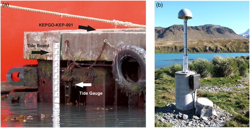
Vertical land movement, arising from whatever combination of geophysical processes, needs to be measured at each tide-gauge site, and the GLOSS programme has a requirement for a GNSS receiver to be installed alongside each tide gauge in its ‘core network’ (IOC 2012). About half of the BOT gauges have been equipped with GNSS so far. For example, Figure 4 shows a GNSS (or Global Positioning System, GPS) installation near to the tide gauge at King Edward Point, South Georgia (Teferle et al. 2014). The Système d'Observation du Niveau des Eaux Littorales (SONEL) website (http://www.sonel.org) contains time series of GNSS measurements at other BOT sites and at many other tide gauges worldwide.

Figure 4. (a) The tide-gauge installation at King Edward Point, South Georgia comprising deep and ‘half-tide’ pressure sensors, a tide board and a tide-gauge benchmark, and (b) a GNSS receiver (called KRSA) approximately 150 m from the tide gauge. The tide gauge, GNSS receiver and an additional receiver on nearby Brown Mountain together form the ‘KEP Geodetic Observatory’, a collaboration between the NOC and the University of Luxembourg.

Source: Photographs courtesy of Professor Norman Teferle, University of Luxembourg.

In spite of the complications to do with vertical land movements, an important point to make with regard to the BOTS is that trends in the last two decades have been positive at every site using either technique (Table 3, with the possible exception of Vernadsky). Although the sea level has actually fallen in this period in some areas, primarily in the eastern Pacific (IPCC 2013; Pugh & Woodworth 2014), the BOTS are all located in the majority part of the ocean where it has risen. It is intentional that the uncertainties in each of the trends in Table 3 are not shown. They are from very short records of only two decades, with gaps in the case of some of the gauge records; they are shown here simply to demonstrate that they have been generally positive. For discussions of trends in the cases where tide-gauge data sets are available for longer periods, see the various publications mentioned above. Similar publications are available concerning UK sea-level trends (Woodworth et al. 2009).

Table 3. Trends in sea level as shown by the altimeter and tide gauge data in Figure 2.

Station number	Altimeter trend in mm/year	Tide-gauge trend in mm/yr
1	2.8	2.9
2	2.0	3.1
3	–	–
4	4.7	2.2
5	2.8	2.7
6	2.4	3.5
7	2.7	1.3
8	3.9	–
9	2.8	1.1
10	1.5	2.6
11	2.4	1.2
12	3.1	3.4
13	3.2	–
14	2.7	–
15	1.9	1.7
16	4.9	5.8
17	2.2	3.9
18	3.7	−0.3

Note: Trends are calculated from the separate red and black data shown in Figure 2. Trends are not shown for altimetry at Rothera (station 3, see text) or for gauges with small amounts of data.

Future sea level and the BOTs

IPCC (2013, Fig. 13.20) shows that the sea-level rise in the Caribbean, South Atlantic and Western Indian Ocean by the end of the twenty-first century could be comparable to the global mean of 26–98 cm, depending upon emission scenario (with the possible exception of the Antarctic stations). This rise will have many impacts (IPCC 2014a, 2014b) and needs to be monitored.

However, if altimetry can provide similar long-term information for the BOTs as tide gauges, why invest in tide gauges at all? The point is that the two sea-level measurement techniques provide highly complementary sets of information, so both are needed. Gauges provide the higher-frequency data needed to monitor the sea level continuously at a particular site, near to where people live or close to environmentally-sensitive coastal ecosystems. In addition, they can be used in ‘multi-purpose’ applications such as tsunami warning. On the other hand, altimeters provide lower-frequency sampling at any one point but more spatially-complete information, giving a synoptic overview of how the sea level is changing in the wider region. The combined analysis of data sets, one source of data being possibly more important than the other in any particular study, provides the authoritative sea-level information required.

There are three further general points to be made in support of the installation of tide gauges. One is that, with regard to long-term trends such as those of Table 3, some people will not accept information from space provided by ‘experts’. If possible, they need the reassurance of knowing that the sea level is rising from local measurements made by their nearest tide gauge. A second point is that space missions cost hundreds of millions of dollars (exactly how much is never clear) compared to the tens of thousands of dollars needed for the establishment of a modern tide gauge (possibly US$50,000 if one also includes a GNSS receiver to monitor land movements, as required by GLOSS standards), so their cost is trivial within that of an overall monitoring system. A third is that, although a number of altimeter missions are assured over the next decade (Benveniste 2011), their high cost means that their availability cannot be guaranteed over the next century, when the sea level is expected to change significantly. The preservation of a relatively low-cost global tide-gauge network is therefore essential in providing continuity of monitoring. However, without national obligations being met (in this case by the BOTs) with regard to an agreed international programme (in this case GLOSS), there is no programme.

Many of the BOTS are located in parts of the ocean that have much less sea-level sampling than, say, Europe or North America. Consequently, their enhanced monitoring of the sea level will be scientifically interesting and novel in many ways. The use of BOT tide gauges to monitor fluctuations in the ACC, which is one of the largest ocean currents, has already been referred to (Hibbert et al. 2010). Further enhanced monitoring in the BOTs will enable oceanographers to understand better the circulation of other remote parts of the ocean. For example, there are plans for a monitoring system of the meridional overturning circulation in the South Atlantic based on a set of mooring across 34.5 deg S (NOAA 2014), similar to that now operational in the North Atlantic (McCarthy et al. 2014). This could be complemented by state-of-the-art sea-level measurements in South America, Africa and at the BOT islands in the southern parts of the South Atlantic. Further north, sea-level data from Ascension and St Helena already add value to the US, French and Brazilian monitoring of the tropical Atlantic (Woodworth et al. 2012; PMEL 2015).

Conclusions

How can all (or at least most) of the BOTs be provided with the sea-level monitoring equipment needed to meet local requirements and fulfil obligations by the UK to a long-term international monitoring programme (i.e., GLOSS)? The difficulty in answering this question stems from the fractured way in which funding is organized in the UK (and the BOTs). The Environment Agency funds the monitoring by the NOC in the UK itself. The Natural Environment Research Council (NERC), of which the NOC is a component, funds the South Atlantic network as part of its science programme (in a subset called ‘National Capability’). Our understanding is that otherwise the lead UK department for international environment observing programmes is the Department for Food, Environment and Rural Affairs (Defra), but they do so only following commitments as a result of signing international conventions, and IOC programmes such as GLOSS do not come into this category. The Foreign and Commonwealth Office has responsibility for the BOTs themselves; it does not fund infrastructure such as that discussed here but nevertheless could do more to encourage the individual BOTs to be better represented in international programmes. To our knowledge, the only BOT to have invested in its own tide gauge has been the Government of Gibraltar a decade ago, although several of the BOTs (or their consultants) have taken the opportunity of making use of NOC-provided data.

Sea-level monitoring is rather better recognized by France regarding its overseas departments and territories. Following the Sumatra tsunami in 2004, both the UK and France commissioned reports on tsunami risk (Kerridge 2005; French Government 2008). However, while the French report was geographically wide-ranging and resulted in major investment in multi-hazard sea-level infrastructure in the Mediterranean and in the territories in the Caribbean, Indian and Pacific Oceans, the UK report was focused on the UK itself and there was no suggestion of corresponding investment in the BOTs. These French investments, although initially concerned with tsunami risk, will eventually benefit all sea-level applications. They were accompanied by an instruction from the Sécrétariat Général à la Mer (directly responsible to the Prime Minister) to extend the remit of the Service Hydrographique et Océanographique de la Marine (SHOM) beyond its traditional hydrographic applications so as to include the coordination of sea-level observations in all departments and territories (French Government 2010). There was no corresponding initiative by the UK.

In our opinion, the UK government should take a similar lead in coordination between UK departments and BOT administrations to ensure that the necessary sea-level monitoring investments take place within its own overseas territories.

Acknowledgements

We are grateful to the Permanent Service for Mean Sea Level (PSMSL) and Brian Beckley (Goddard Space Flight Center, National Aeronautics and Space Administration) for the tide-gauge and altimeter data sets used in this paper. Peter Foden and Jeff Pugh (NOC) are thanked for their many contributions to the sea-level monitoring in the BOTs. David Pugh (NOC), Guy Wöppelmann (University of La Rochelle) and Norman Teferle (University of Luxembourg) provided valuable advice.

Disclosure statement

No potential conflict of interest was reported by the authors.

References

- Benveniste J. 2011. Radar altimetry: past present and future. pp. 1–17 in Coastal Altimetry (eds. Vignudelli S et al). Berlin: Springer-Verlag, 565pp.
- Cannon J. 2009. A dictionary of British history. Oxford: Oxford University Press, 720pp.
- Dunne RP, Barbosa SM, Woodworth PL. 2012. Contemporary sea level in the Chagos Archipelago, central Indian Ocean. Global Planet Change. 82–83:25–37. doi:10.1016/j.gloplacha.2011.11.009.
- French Government. 2008. http://www.senat.fr/notice-rapport/2008/r08-546-notice.html
- French Government. 2010. http://www.sonel.org/IMG/pdf/SGMER863_2010.pdf
- Garrett C, Akerley J, Thompson K. 1989. Low-frequency fluctuations in the strait of gibralter from MEDALPEX sea level data. J Phys Oceanogr. 19:1682–1696. doi:10.1175/1520-0485(1989)019<1682:LFFITS>2.0.CO;2.
- Herschel JFW. editor. 1849. A manual of scientific enquiry; prepared for the use of her majesty's navy; and travellers in general. London: John Murray (Publisher to the Admiralty), 488pp.
- Hibbert A, Leach H, Woodworth PL, Hughes CW, Roussenov VM. 2010. Quasi-biennial modulation of the Southern Ocean coherent mode. Q J Roy Meteo Soc. 136:755–768. doi:10.1002/qj.581.
- Hughes CW, Woodworth PL, Meredith MP, Stepanov V, Whitworth T, Pyne AR. 2003. Coherence of Antarctic sea levels, Southern Hemisphere annular mode, and flow through drake passage. Geophys Res Lett. 30:1464. doi:10.1029/2003GL017240.
- IOC. 2006. Manual on sea-level measurement and interpretation. Volume 4 – An update to 2006. (eds. Aarup, T., Merrifield, M., Perez, B., Vassie, I and Woodworth, P.). Intergovernmental Oceanographic Commission Manuals and Guides No. 14. IOC, Paris, 80pp.
- IOC. 2012. The global sea level observing system (GLOSS) implementation plan – 2012. UNESCO/Intergovernmental Oceanographic Commission. 37pp. (IOC Technical Series No. 100). Available from ioc.unesco.org.
- IPCC. 2013. Climate change 2013: the physical science basis. contribution of working group i to the fifth assessment report of the intergovernmental panel on climate change (eds. Stocker TF et al.). Cambridge: Cambridge University Press, 1535pp.
- IPCC. 2014a. Climate change 2014: impacts, adaptation, and vulnerability. Part A: global and sectoral aspects. contribution of working group ii to the fifth assessment report of the intergovernmental panel on climate change (eds. Field CB et al.). Cambridge: Cambridge University Press, 1132pp.
- IPCC. 2014b. Climate change 2014: impacts, adaptation, and vulnerability. Part B: regional aspects. contribution of working group ii to the fifth assessment report of the intergovernmental panel on climate change (eds. Barros VR et al.). Cambridge: Cambridge University Press, 688pp.
- Kenworthy JM, Walker JM. editors. 1997. Colonial observatories and observations: meteorology and geophysics. Proceedings of a conference held at St. Mary's College, University of Durham, 8–10 April 1994. Durham University, Department of Geography, Occasional Publication No. 31. Durham: University of Durham and London: Royal Meteorological Society. 214pp.
- Kerridge D. 2005. The threat posed by tsunami to the UK. Study commissioned by Defra flood management and produced by the British Geological Survey, Proudman Oceanographic Laboratory, Met Office and HR Wallingford. 167pp.
- Mathers EL, Woodworth PL. 2004. A study of departures from the inverse-barometer response of sea level to air-pressure forcing at a period of 5 days. Q J Roy Meteor Soc. 130: 725–738. doi:10.1256/qj.03.46.
- McCarthy GD, Smeed DA, Johns WE, Frajka-Williams E, Moat BI, Rayner D, Baringer MO, Meinen CS, Collins J, Bryden HL. 2014. Measuring the Atlantic Meridional overturning circulation at 26°N. Prog Oceanogr. 130:91–111. doi:10.1016/j.pocean.2014.10.006.
- Menemenlis D, Fukumori I, Lee T. 2007. Atlantic to Mediterranean sea level difference driven by winds near Gibraltar strait. J Phys Oceanogr. 37:359–376. doi:10.1175/JPO3015.1.
- Meredith MP, Woodworth PL, Hughes CW, Stepanov V. 2004. Changes in the ocean transport through Drake Passage during the 1980s and 1990s, forced by changes in the Southern annular mode. Geophys Res Lett. 31:L21305. doi:10.1029/2004GL021169.
- Mitchum GT. 2000. An improved calibration of satellite altimetric heights using tide gauge sea levels with adjustment for land motion. Mar Geod. 23:145–166. doi:10.1080/01490410050128591.
- NOAA. 2014. South Atlantic meridional overturning circulation (SAMOC). National Oceanic and Atmospheric Administration. Atlantic Oceanographic and Meteorological Laboratory. Available from: http://www.aoml.noaa.gov/phod/research/moc/samoc/
- PMEL. 2015. Pacific marine environmental laboratory of NOAA. Prediction and Research Moored Array in the Atlantic (PIRATA) web pages. Available from: http://www.pmel.noaa.gov/pirata
- Pugh DT, Woodworth PL. 2014. Sea-level science: understanding tides, surges, tsunamis and mean sea-level changes. Cambridge: Cambridge University Press. ISBN 9781107028197. 408pp.
- Sturges W, Hong BG. 1995. Wind forcing of the Atlantic thermocline along 32 deg N at low frequencies. J Phys Oceanogr. 25:1706–1715. doi:10.1175/1520-0485(1995)025<1706:WFOTAT>2.0.CO;2.
- Tamisiea ME, Mitrovica JX. 2011. The moving boundaries of sea level change: understanding the origins of geographic variability. Oceanography. 24:24–39. doi:dx.doi.org/10.5670/oceanog.2011.25.
- Teferle FN, Hunegnaw A, Ahmed F, Sidorov D, Woodworth PL, Foden PR, Williams SDP. 2014. The king Edward point geodetic observatory, South Georgia, South Atlantic Ocean. A first evaluation and potential contributions to geosciences. Proceedings of the IAG Symposium, Potsdam, 2013. (Springer Publishing, in press).
- Thompson PR, Mitchum GT. 2014. Coherent sea level variability on the North Atlantic western boundary. J Geophys Res. 119. doi:10.1002/2014JC009999.
- Vassie JM, Woodworth PL, Holt MW. 2004. An example of North Atlantic deep ocean swell impacting Ascension and St. Helena islands in the central South Atlantic. J Atmos Ocean Tech. 21:1095–1103. doi:10.1175/1520-0426(2004)021<1095:AEONAD>2.0.CO;2.
- Vinogradov SV, Ponte RM. 2011. Low-frequency variability in coastal sea level from tide gauges and altimetry. J Geophys Res. 116:C07006. doi:10.1029/2011JC007034.
- Wikipedia. 2014. http://en.wikipedia.org/wiki/British_Overseas_Territories
- Williams J, Hughes CW. 2013. The coherence of small island sea level with the wider ocean: newline a model study. Ocean Sci. 9:111–119. doi:10.5194/os-9-111-2013.
- Woodworth PL, Foden PR, Jones DS, Pugh J, Holgate SJ, Hibbert A, Blackman DL, Bellingham CR, Roussenov VM, Williams RG. 2012. Sea level changes at Ascension Island in the last half century. Afr J Mar Sci. 34:443–452. doi:10.2989/1814232X.2012.689623.
- Woodworth PL, Hughes CW, Blackman DL, Stepanov VN, Holgate SJ, Foden PR, Pugh JP, Mack S, Hargreaves GW, Meredith MP, et al. 2006. Antarctic Peninsula sea levels: a real time system for monitoring Drake Passage transport. Antarct Sci. 18:429–436. doi:10.1017/S0954102006000472.
- Woodworth PL, Morales Maqueda MA, Roussenov VM, Williams RG, Hughes CW. 2014. Mean sea-level variability along the northeast American Atlantic coast and the roles of the wind and the overturning circulation. J Geophys Res. 119. doi:10.1002/2014JC010520.
- Woodworth PL, Pugh DT, Bingley RM. 2010. Long term and recent changes in sea level in the Falkland Islands. J Geophys Res. 115:C09025. doi:10.1029/2010JC006113.
- Woodworth PL, Pugh DT, Meredith MP, Blackman DL. 2005. Sea level changes at Port Stanley, Falkland Islands. J Geophys Res. 110:C06013. doi:10.1029/2004JC002648.
- Woodworth PL, Teferle N, Bingley R, Shennan I, Williams SDP. 2009. Trends in UK mean sea level revisited. Geophys J Int. 176:19–30. doi:10.1111/j.1365-246X.2008.03942.x.
- Woodworth PL, Vassie JM, Spencer R, Smith DE. 1996. Precise datum control for pressure tide gauges. Mar Geod. 19:1–20. doi: 10.1080/01490419609388068
- Woodworth PL, Windle SA, Vassie JM. 1995. Departures from the local inverse barometer model at periods of 5 days in the central South Atlantic. J Geophys Res. 100(C9):18281–18290. doi:10.1029/95JC01741.