The Copernicus Marine Environment Monitoring Service Ocean State Report

ABSTRACT

The Copernicus Marine Environment Monitoring Service (CMEMS) Ocean State Report (OSR) provides an annual report of the state of the global ocean and European regional seas for policy and decision-makers with the additional aim of increasing general public awareness about the status of, and changes in, the marine environment. The CMEMS OSR draws on expert analysis and provides a 3-D view (through reanalysis systems), a view from above (through remote-sensing data) and a direct view of the interior (through in situ measurements) of the global ocean and the European regional seas. The report is based on the unique CMEMS monitoring capabilities of the blue (hydrography, currents), white (sea ice) and green (e.g. Chlorophyll) marine environment. This first issue of the CMEMS OSR provides guidance on Essential Variables, large-scale changes and specific events related to the physical ocean state over the period 1993–2015. Principal findings of this first CMEMS OSR show a significant increase in global and regional sea levels, thermosteric expansion, ocean heat content, sea surface temperature and Antarctic sea ice extent and conversely a decrease in Arctic sea ice extent during the 1993–2015 period. During the year 2015 exceptionally strong large-scale changes were monitored such as, for example, a strong El Niño Southern Oscillation, a high frequency of extreme storms and sea level events in specific regions in addition to areas of high sea level and harmful algae blooms. At the same time, some areas in the Arctic Ocean experienced exceptionally low sea ice extent and temperatures below average were observed in the North Atlantic Ocean.

KEYWORDS:

• Copernicus Marine Environment Monitoring Service
• Ocean reporting
• Ocean monitoring
• State of the ocean
• Ocean variability
• Operational oceanography
• Ocean climate variability

Introduction

Our Earth is a blue planet. The world’s oceans cover about 71% of the Earth’s surface and 90% of the Earth’s biosphere, and contain 97% of the Earth’s water. They provide essential services to society such as food and energy and a play a major part in economic activities. The oceans play a central role in regulating the Earth’s climate, in particular its variability and change, through its ability to absorb and transport large quantities of heat, moisture, carbon and other biogeochemical gases around the planet (IPCC 2013). Since the beginning of the industrial period, the Earth’s climate has come under anthropogenic pressure. The key factors are increases in carbon dioxide (CO₂) from burning fossil fuels and emissions of other greenhouse gases and radiative active aerosols (e.g. Hansen et al. 2011). The world’s oceans act as an energetic and biogeochemical buffer. Over the last 50 years, they have absorbed more than 90% of the excess heat received by our warming planet (Levitus et al. 2005). At the same time, they have absorbed nearly 30% of anthropogenic CO₂ emissions leading to ocean acidification (Le Quéré et al. 2015). These human-induced changes interfere with the natural flow of energy in the climate system. The major buffering effects of the ocean on the climate are not without consequences on the ocean physics and chemistry: sea level rise, increase in temperatures at the surface and at depth, sea ice melting and shrinking of the Arctic sea ice, de-oxygenation and expansion of oxygen minimum zones and acidification. These changes in the physical and chemical ocean parameters have already had a large impact on marine habitats, ecosystems and marine resources, which are also subject to strong pressures from other human activities, including pollution, fishing and resource extraction (IPCC 2014).

The Copernicus Marine Environment Monitoring Service (CMEMS) Ocean State Report (OSR) is conceived as an annual reporting of the state and health of the global ocean and regional seas based on unique CMEMS marine environment monitoring capabilities. The OSR will deliver a regular monitoring of the blue (hydrography, currents), white (sea ice) and green (e.g. Chlorophyll) marine environment and spans time scales from decadal trends, interannual, seasonal and subseasonal changes through to near-real-time monitoring. The aim is to increase general public awareness about the marine environment, its environmental status and its potential in terms of resources. This is achieved by CMEMS expert analysis on the state, variability and change of the global ocean and the European regional seas through a 3-D ocean view (reanalysis systems), a view from above (remote-sensing data) and a direct view into the ocean’s interior (in situ measurements).

There is now, more than ever, a need for more systematic ocean information, which was very much acknowledged during the twenty-first session of the Conference of the Parties (COP21) and led to the decision to develop a special report by the Intergovernmental Panel on Climate Change (IPCC) on Climate Change, Oceans and Cryosphere. Observing and monitoring the oceans is also essential for better and more sustainable management of our oceans and seas in support of the development of human activities and of the blue economy. This is recognised in the United Nations sustainable development goal 14 (SDG 14) that aims to ‘conserve and sustainably use the oceans, seas and marine resources for sustainable development’. The CMEMS was set up to propose a pan-European contribution to these challenges. The development of annual Ocean State Reports by the CMEMS is one of the priority tasks allocated by an EU delegation agreement for the CMEMS implementation (CMEMS 2014). Such reports and their associated ocean monitoring indices are expected to serve and contribute to European agencies or organisations in charge of environmental monitoring (e.g. the European Environment Agency (EEA), OSPAR, the Baltic Marine Environment Protection Commission, United Nations Environment Programme Mediterranean Action Plan (Unep-Map)), European directives such as the Marine Strategy Framework Directive (MSFD), international fishery management agencies (International Council for Exploration of the Seas (ICES), Food and Agricultural Organization (FAO)), to the Copernicus Climate Change Service (C3S) and to international groups, agencies or programs responsible for assessing the climate of the Earth and of the ocean (e.g. IPCC, Intergovernmental Oceanographic Commission of the United Nations Educational, Scientific and Cultural Organization (IOC of UNESCO), World Climate Research Program, Future Earth, United Nations World Ocean Assessment and the Group on Earth Observations).

The CMEMS vision is that of a ‘World-leading marine environment and monitoring service in support of blue growth and economy for maritime safety, effective use of marine resources, healthy waters, information for coastal and marine hazard services, and assistance for climate services’ (CMEMS 2016). Following the successful completion of the MyOcean1&2 and follow on research and development projects, Mercator Ocean was tasked in 2014 by the EU under a delegation agreement to implement the operational phase of the service from 2015 to 2021 (CMEMS 2014). The CMEMS organisation is based on a strong European partnership with more than 50 marine operational and research centres in Europe involved in the service and its evolution. The CMEMS provides regular and systematic reference information on the physical state, variability and dynamics of the ocean and marine ecosystems for the global ocean and the European regional seas (Figure 1). This capacity encompasses the description of the current situation (analysis), the prediction of the situation a few days ahead (forecast) and the provision of consistent retrospective data records for recent years. The CMEMS mission includes:

• Observations, monitoring and reporting on past and present marine environmental conditions, in particular, the response of the oceans to climate change and other stressors;

• Analysing and interpreting changes and trends in observations and measurements of the marine environment;

• Provision of short-term forecasts and outlooks for marine conditions and, as appropriate, to downstream services for warnings of and/or rapid responses to extreme or hazardous events;

• Provision of detailed descriptions of the ocean state, variability and change to initialise coupled ocean/atmosphere models to predict changes in the atmosphere/climate.

The CMEMS provides a sustained and sustainable response to European users’ needs in four application areas: (i) maritime safety, (ii) marine resources, (iii) coastal and marine environment and (iv) weather, seasonal forecast and climate. A major objective of the CMEMS is to deliver and maintain a competitive and state-of-the-art European service responding to public and private intermediate user needs. The CMEMS includes both satellite and in situ high-level products prepared by Thematic Assembly Centres (TACs) and modelling and data assimilation products prepared by Monitoring and Forecasting Centres (MFCs).¹ CMEMS products are based on state-of-the-art data processing and modelling techniques. Products are described in product user manuals (PUMs). Internationally recognised verification and validation procedures are used to assess product quality (e.g. Hernandez et al. 2015). They are carried on at each upgrade of the CMEMS production systems (MFCs or TACs) and the overall quality of each product is monitored through regular review and routine operational verification (http://marine.copernicus.eu/services-portfolio/validation-statistics/). Quality information documents (QuIDs) detail these validation procedures and provide an estimate on the product accuracy and reliability. The PUMs and QuIDs are available for each CMEMS product and can be downloaded from the CMEMS online portal (http://marine.copernicus.eu/).

Figure 1. Schematic overview on data products used in the CMEMS OSR. Three types of multi-year products for the global ocean and regional seas (see map) are distributed in the CMEMS catalogue, i.e. ocean reanalysis (RAN) products, reprocessed in situ products and reprocessed satellite products. ESA-CCI products were also used to complement CMEMS multi-year satellite products. Time series generally start from the year 1993 and are extended close to real time through the additional use of CMEMS near-real-time products. See text for more details. CMEMS geographical areas on the map are for: 1 – Global Ocean; 2 – Arctic Ocean from 62°N to North Pole; 3 – Baltic Sea, which includes the whole Baltic Sea including Kattegat at 57.5°N from 10.5°E to 12.0°E; 4- European North-West Shelf Sea, which includes part of the North-East Atlantic Ocean from 48°N to 62°N and from 20°W to 13°E. The border with the Baltic Sea is situated in the Kattegat Strait at 57.5°N from 10.5°E.to 12.0°E; 5 – Iberia-Biscay-Ireland Regional Seas, which include part of the North-East Atlantic Ocean from 26°N to 48°N and 20°W to the coast. The border with the Mediterranean Sea is situated in the Gibraltar Strait at 5.61°W; 6- Mediterranean Sea, which includes the whole Mediterranean Sea until the Gibraltar Strait at 5.61°W and the Dardanelles Strait; 7- Black Sea, which includes the whole Black Sea until the Bosphorus Strait.

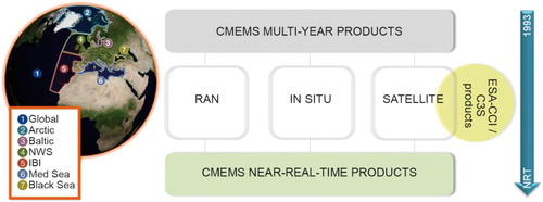
The CMEMS thus gathers unique capability and expertise in Europe to monitor and assess the state, variability and change of the oceans. The integrated (satellite and in situ observations, modelling and data assimilation) monitoring of the global ocean and European seas organised by CMEMS is, in particular, a major asset for organising a regular reporting of the ocean state and health. The report relies on the exploitation of data sets during the period 1993–2015 both from ocean reanalysis and analysis systems and observations (in situ and remote sensing, Figure 1). All CMEMS products analysed in the report are considered to be properly documented, assessed and reliable for scientific analysis as detailed in their corresponding PUMs and QUIDs. Experts contributing to this report have deliberately chosen the most appropriate CMEMS products to infer the required ocean properties. The products are called ‘multi-year’ products, which rely on ocean reanalysis (global and regional), reprocessed in situ observational products or reprocessed satellite products (Figure 1). CMEMS multi-year products are part of the CMEMS strategy that supports users’ needs with ocean time series and description over the last three decades (the ‘satellite’ era), in order to complement the operational daily hindcasts/short-term forecasts provision. The reliability and quality of these multi-year products are higher than operational ones. They benefit from reprocessed and delayed-time upstream data (forcings, observations) and better-suited and tailored modelling and estimation tools. However, the reprocessed satellite products may not be considered as ‘climate records’, and the analysis is complemented by using additional products from the European Space Agency-Climate Change Initiative (ESA-CCI, http://cci.esa.int/) and from the Copernicus Climate Change Service if available (Figure 1). Their use is clearly indicated in this report. In order to achieve continuity and state-of-the-art information, most of the multi-year products have been complemented with operational products over the recent years –called ‘near-real-time (NRT) products’ (Figure 1).

The report is divided into four principal chapters and is focused on monitoring (state, variability and change) of the physical ocean during the period 1993–2015 for the global ocean and the European regional seas (Figure 1). Reporting is based on peer-reviewed state-of-the-art scientific results, analyses and methodologies. This report is the first one produced by the CMEMS and will be followed by regular annual releases towards the end of each year. As the CMEMS and its monitoring capabilities develop, subsequent releases will include additional syntheses, in particular related to biogeochemistry and marine ecosystem changes (e.g. oxygen depletion, CO₂ fluxes, acidification, primary production). The first chapter discusses a selection of Essential Ocean/Climate Variables. Chapter 2 further deepens this reporting with an analysis on large-scale changes of the physical ocean. Chapter 3 is focused on circulation and hydrographic changes in the CMEMS regions (Figure 1) – except for the Black Sea recently added in the frame of the CMEMS, and for which a dedicated regional reporting will be added in next year’s OSR. Chapter 4 addresses some of the major climate and marine environmental events. A fundamental part of the CMEMS OSR concept relies on the aim to deliver a synthesised view on selected topics and to avoid lengthy description and scientific review. All sections have been limited in length, and existing topic scientific review assessments have been cited whenever available.

Chapter 1: Essential variables

There is a growing need for more systematic ocean information to support efforts to manage our relationship with the ocean. This is also required to understand and predict the evolution of the climate, in order to guide mitigation and adaptation measures, to assess risks and enable attribution of climatic events to underlying causes, and to underpin climate services (Bojinski et al. 2014). To provide guidance, the Global Climate Observing System (GCOS 2011) and the Global Ocean Observing System (GOOS) programs developed the concept of ‘Essential Climate Variables’ (ECVs) and ‘Essential Ocean Variables’ (EOVs, see also http://ioc-goos-oopc.org/obs/ecv.php) that are required to support the work of the United Nations Framework Convention on Climate Change and the IPCC (ECVs) but also to monitor the health of the oceans and support many ocean services (for EOVs). They are physical, chemical or biological variables that critically contribute to the characterisation of Earth’s climate and of the oceans. This concept has been broadly adopted in science and policy circles (IFSOO 2012). This chapter on essential variables of the CMEMS OSR 2016 aims at responding to the need for faster and better-coordinated information in order to support both research and societal needs.

Seven different essential variables – most of them classified as ECVs/EOVs – are discussed in this OSR, i.e. sea surface temperature, subsurface temperature, surface and subsurface salinity, sea level, ocean colour Chlorophyll-a, currents, and sea ice. This is a dedicated and unique effort of the European scientific and operational oceanography communities. It provides a complementary perspective focused on the ocean (global and European regional seas) in parallel to the more exhaustive special Bulletin on the state of the climate of the American Meteorological Society (e.g. Blunden & Arndt 2016). State, variability and change of the seven essential variables during the period 1993–2015 are analysed using CMEMS and ESA-CCI products at global and regional scales. For most of the essential variables presented here, a specific focus on changes during the year 2015 is given. This first chapter is an important part of the CMEMS OSR and is expected to expand with the evolution of this activity. More precisely, the aim is to develop a unique reference in the near future through the development of a coherent and harmonised (temporal and regional, see Section 1.4 as an example) reporting of essential variables based on the CMEMS physical and biogeochemical products. The results presented here are a first but fundamental step towards this much needed objective.

1.1. Sea surface temperature

Leading authors: Hervé Roquet, Andrea Pisano, Owen Embury.

Contributing authors: Simon Good, Rebecca Reid, John Kennedy, Bruno Buongiorno Nardelli, Fabrice Hernandez.

Sea surface temperature (SST) is the key oceanic variable determining the exchange of heat between ocean and atmosphere. It is one of the basic parameters in research and prediction of climate variability and change, and is also required for many other applications, such as meteorological and ocean forecast systems (e.g. Chelton & Wentz 2005), diurnal warming cycle reconstruction (e.g. Marullo et al. 2014), aquaculture etc. SST can provide insight into the heat balance in the climate system, general circulation patterns and thermal anomalies. Atmospheric water content and wind near the surface both depend on SST which, in turn, provides information about the presence of fronts between different water masses and about the intensity of coastal and equatorial upwelling. It has been routinely measured from space since the late 1970s by a variety of Earth Observation satellites and instruments, with a typical accuracy of 0.5°C when compared with routine drifting buoy measurements (e.g. Marsouin et al. 2016). Recently, the ESA-CCI – has been focusing on the reprocessing of long time series of satellite-derived SST for climate applications, to provide data sets with improved accuracy and stability compared to near-real-time products (Merchant et al. 2014).

Time series of SST monthly global mean anomalies for the period 1993–2015 have been derived from the satellite-derived ESA-CCI observational products.² Results exhibit an obvious SST warming at a rate of 0.016°C/yr ± 0.002 at 99% significance (Figure 2(a), see also Stocker et al. 2013), which corresponds to an average total increase of about 0.4°C over this 23-year period (note that the Mann–Kendall test is used to estimate the confidence in the sign of the time series, and Sen’s method to estimate the slope of the time series, see Mann 1945; Sen 1968; Kendall 1975). Superimposed on this long-term change in global mean SST trend are variations at an interannual time scale. These changes are mostly related to strong signatures of El Niño Southern Oscillation (ENSO, see Section 4.1) variability, with a particular strong increase in SST during the 2015 El Niño event.

Figure 2 (a) SST monthly global mean anomaly time series based on the ESA-CCI product (see text for details) (b) Mediterranean and (c) Black Sea SST monthly mean anomaly time series (see text for more details on data use). Dedicated assessment during the overlapping period between the reprocessed and near-real-time product (2008–2012) shows the consistency between the two SST time records. Major biases between the reprocessed and near-real-time products have been removed from the latter for the recent years.

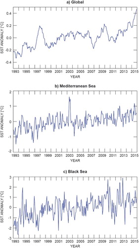
For the Mediterranean and Black Seas, the CMEMS reprocessed satellite regional product (Pisano et al. 2016) has been used³ from 1993 to 2013, and extended by the CMEMS near-real-time product.⁴ SST minima in the Mediterranean Sea were recorded during 1993 and 1996, while maximum SST values occurred during summer 2003 (see also Jung et al. 2006; Feudale & Shukla 2007) and 2015 (Figure 2(b)). Mediterranean Sea mean SST increased at a rate of 0.039 ± 0.009°C/yr (99% significance level), which corresponds to an average increase of 0.9°C over the 1993–2015 period. A much stronger SST increase is observed in the Black Sea over the same period at a rate of 0.082 ± 0.018°C/yr and an average increase of 1.9°C over the 23-year period. The SST trend estimated for the Black Sea is in accordance with a previously estimated rate of 0.075°C/yr over the period 1985–2005 (Buongiorno Nardelli et al. 2010). The strong differences in the Black Sea mean SST anomaly variability compared to that in the Mediterranean Sea is probably due to the alternate and competing meteorological influences of the cold Siberian anticyclone and the milder Mediterranean weather system on the Black Sea (Shapiro et al. 2010).

In order to discuss changes during the year 2015, anomalies have been obtained from the CMEMS near-real-time satellite product⁵ against climatology (1993–2007) based on the CMEMS reprocessed satellite product.⁶ In 2015, the global mean SST anomaly (Figure 3(a)) shows three features of particular interest: a warm anomaly in the Equatorial Pacific, related to the 2015 El Niño; a warm anomaly in the eastern part of the North Pacific and a cold anomaly in the North Atlantic. This El Niño event (see Section 4.1) is comparable in strength to the 1997/98 El Niño, but the peak in temperature anomalies is further to the west than it was in 1997. The warm SST anomaly extends along the equator east of 180°W as well as along the coast of Peru up to 15°S, with values exceeding 2°C. The warm anomaly in the Northeast Pacific developed in winter 2013/14, strengthened during 2014 and lasted through 2015. The formation of the anomaly was associated with a strong and persistent high-pressure pattern in the area during the winter (which may also have helped to lower SSTs in the North Atlantic). The anomaly is correlated with the positive phase of the Pacific Decadal Oscillation (PDO) (Newman et al. 2003). The PDO has been in a generally negative phase over the last decade and the current conditions might herald a return to the positive phase. In contrast, the Atlantic Multi-decadal Oscillation (AMO) has been in its positive phase (warmer than average SSTs in the north Atlantic) since the mid-1990s. In the North Atlantic, a cold anomaly was observed, lying in an area south of Greenland and Iceland (see also chapter 4). By some measures, summer temperatures in the region were the coldest since records began. Lower SSTs in other parts of the North Atlantic could represent the first signs of a switch to cooler conditions and the negative phase of the AMO. Overall, Northern hemisphere SSTs were exceptionally high in 2015.

Figure 3 (a): Yearly-mean global 2015 SST anomaly map (−3/ + 3°C, see text for information on data use) relative to the 1993–2007 climatology. Specific comparison between the near-real-time and reprocessed SST estimates shows maximum differences of around 0.6°C, except in very specific locations (Roberts-Jones et al. 2011). Hence, this analysis is relevant for demonstrating features whose amplitude is significantly greater than 1°C. (b): Same as (a), but over the Black Sea and Mediterranean Sea (−1.5/ + 1.5°C).

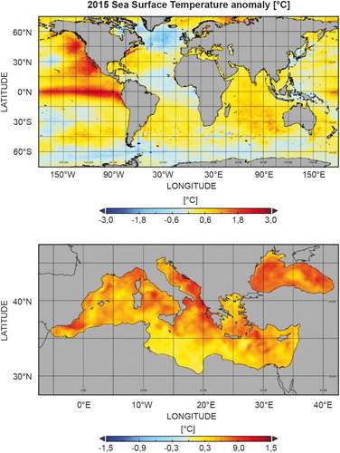
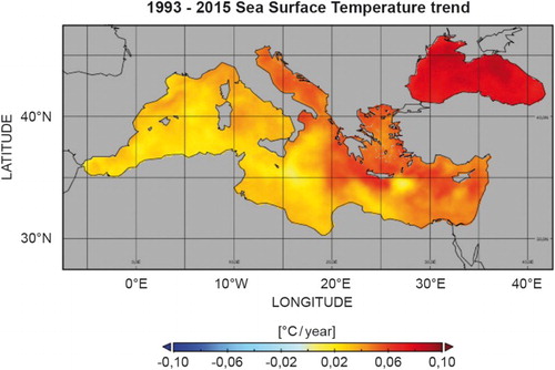
Figure 3(b) reveals a general surface warming anomaly during 2015 over the whole Mediterranean and Black Seas. In particular, the Northern Mediterranean basin and the entire Black Sea experienced a strong positive anomaly (represented by colours in a shade of red for anomalies larger than 0.8°C), while anomalies along the Libyan coast were close to zero. The spatial pattern of the SST trend (Figure 4) over the 1993–2015 time period is consistent with this general surface warming and shows a distinct behaviour between the western and eastern sides of the Mediterranean Sea. Indeed, the magnitude of the trend increases moving eastwards, with minima in the western basin and maxima in the Cretan Arc and in the North Aegean Sea.

Figure 4. 1993–2015 SST trend map in degrees Celsius per year, over the Black Sea and Mediterranean Sea, derived from the same data set as in Figure 3.

1.2 Subsurface temperature

Leading authors: Stephanie Guinehut, Simona Simoncelli.

Contributing authors: Sandrine Mulet, Nathalie Verbrugge, Karina von Schuckmann.

Subsurface temperature is a key EOV from which the ocean heat storage (see Section 2.1) and transport can be deduced (see Section 2.2). Large-scale temperature variations in the upper layers are mainly related to the heat exchange with the atmosphere and surrounding oceanic regions, while the deeper ocean temperature in the main thermocline varies due to many dynamical forcing mechanisms and also to climate change (e.g. Forget & Wunsch 2007; Roemmich et al. 2015; Riser et al. 2016). Subsurface temperatures have been analysed from the CMEMS reprocessed product⁷ combining satellite observations and in situ observations. For the global ocean, estimates of depth-dependent changes in temperature (Figure 5(a)) for the 1993–2015 period range from −0.2°C at the beginning of the period to 0.2°C in 2015. The upper 100 m temperature anomaly tracks the global SST anomaly (see Section 1.1, Figure 2(a)). The 100–400 m layer is dominated by the variability of the depth and slope of the Equatorial Pacific thermocline (e.g. Roemmich & Gilson 2011). Since 2013, the anomalies have been positive from the surface down to 800 m depth. The ocean was warming also at deeper layers (> 700 m depth) at a rate of about 0.003°C/yr over the period 1993–2015 (Figure 5(b)).

Figure 5 (a) Depth/time section of globally averaged subsurface temperature (T) anomalies during the period 1993–2015 and relative to the climatological period 1993–2014 (in °C, contour interval is 0.01 for colours, 0.05 in black) and (b) Depth/latitude section of zonally averaged subsurface temperature trends during the period 1993–2015 (in °C/year, contour interval is 0.0025 for colours, the black line corresponds to the area where the formal error adjustment of the least-square fit is greater than 0.005°C/year), see text for more details on data use.

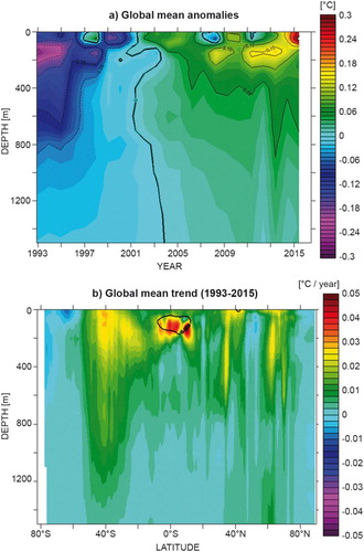
The amplitude of the warming is not spatially uniform (Figure 5(b); von Schuckmann et al. 2009; Guinehut et al. 2012). The Southern Oceans exhibit a strong trend down to 1400 m depth at rates of up to 0.025°C/yr in the top 400 m. Wijffels et al. (2016) indicate further that the southern hemisphere heats at a rate about four times faster than the Northern hemisphere, the latter being the strongest contributor to changes in global Ocean Heat Content (OHC) (see Section 2.1). In the tropics, the signal is dominated by the strong interannual variability of the Equatorial Pacific thermocline with a succession of deepening and outcropping in response to El Niño Southern Oscillation (ENSO, see Section 4.1). Maximum rate values of 0.05°C/yr are reached there. They are associated with maximum values of 0.005°C/yr in the formal error adjustment of the least-square fit. In the Northern Hemisphere, variability patterns appear to be much more complex, with a succession of warming and cooling trends at mid and high latitudes making the global trend a patchier field. It is thus necessary to study more precisely what is occurring separately in the Atlantic and Pacific Oceans considering also that they have very different water mass properties (e.g. Talley 2008).

Focusing on the year 2015, a warm anomaly up to 0.5°C occurs in the three Southern Ocean basins between 60°S and 20°S, in particular in the upper 400 m depth of the Pacific and Indian Oceans (Figure 6). Strong baroclinic variability is visible in the Equatorial Pacific Ocean (Figure 6(b)) with anomalies of opposite sign: positive at the surface up to 2°C and negative at the subsurface up to −2.5°C. This is due to the strong ENSO event that peaked during 2015 (see Section 4.1). The Indian Ocean (Figure 6(c)) shows homogeneous positive anomalies in the equatorial region for the top 400 m with mean amplitude of 0.5°C reaching 1.5°C in the main thermocline. As for the previous two years (2013 and 2014, not shown), the Equatorial Atlantic Ocean shows no remarkable signals.

Figure 6. Depth/latitude sections of subsurface temperature anomalies in 2015 relative to the climatological period 1993–2014. Averages are given for (a) the Atlantic Ocean, (b) the Pacific Ocean, (c) the Indian Ocean and (d) the Mediterranean Sea. Units are °C, contour interval is 0.05, except for the two extreme colours. See text for more details on the data use.

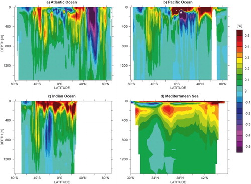
The 2015 anomalies in the North-Eastern Pacific Ocean show shallow but strong positive anomalies of 0.6°C in the first 200 m depth layer as already reported by Bond et al. (2015). This pattern is associated with a positive phase of the PDO: http://research.jisao.washington.edu/pdo/PDO.latest. In the North Atlantic Ocean anomalies are positive and of the order of 0.4°C between 20°N and 40°N and reach down to 800 m depth. They are then strongly negative between 40°N and 65°N with maximum values of −1°C in the first 200 m depth layer. These strong negative temperatures have been related to a strong cooling event which is further described in Section 4.2 (see also Grist et al. 2016). Further north, the anomalies are again positive and around 0.2°C.

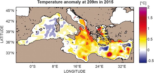
The CMEMS areas of the North Atlantic Ocean, namely Iberian-Biscay-Irish (IBI) and North-West Shelf (NWS), are affected by the strong cooling event described further in Section 4.2. In particular, offshore regions of NWS show negative anomalies of −0.5°C down to 1200 m. For the Mediterranean Sea analysis in Figure 7, the CMEMS regional renalaysis product for the 1993 to 2014 period⁸ was used, and the time series extended using the CMEMS regional near-real-time analysis product for the year 2015.⁹ In the Mediterranean Sea, mean positive anomalies of 0.3°C are observed at the surface and also centred at 200 m. A smaller warming of 0.1°C is also visible down to 700 m (Figure 6(d)). Near 200 m (Figure 7) large positive anomalies characterise the flanks of the Northern Ionian, eastern coast of the Southern Adriatic and the northwestern Aegean, while in the Levantine basin they mark the Mersa-Matruh Gyre, the Shikmona Gyre System and the Gulf of Antalya. The largest negative anomalies (not visible in the depth/latitude section) are visible southeast of Crete where the Ierapetra Gyre is generally located although in 2015 it was absent (see also Sections 2.4 and 3.1), and east of Cyprus Island where it coincides with the Latakia Eddy (Menna et al. 2012).

Figure 7. Temperature anomalies at 209 m in 2015 relative to the climatological period 1993–2014 for the Mediterranean Sea, see text for more details on the data use. Units are °C.

1.3. Surface and subsurface salinity

Leading authors: Stephanie Guinehut, Giulio Notarstefano, Simona Simoncelli, Pierre-Marie Poulain and Karina von Schuckmann.

Contributing authors: Sandrine Mulet, Nathalie Verbrugge.

Ocean salinity is a very important EOV as it is linked to the Earth’s water cycle, and is a key element of weather, climate and environmental systems. The largest component of the global water cycle occurs at the ocean–atmosphere interface (Trenberth et al. 2007). Moreover, shifts in the oceanic distribution of saline and fresh waters are occurring worldwide suggesting links to global warming and possible changes in the hydrological cycle of the Earth (Curry et al. 2003; Durack et al. 2016).

The spatial structure of the global ocean surface and subsurface salinity field is maintained by ocean circulation and mixing, which are both driven by ocean density gradients and air–sea fluxes. At this interface, sea surface salinity (SSS) responds to changing evaporation, precipitation and river runoff patterns by displaying salty or fresh anomalies. It has long been noted that the climatological mean SSS and the surface Evaporation–Precipitation-River runoff (E-P-R) flux field (Josey et al. 2013) are highly correlated (Wüst 1936), which reflects the long-term balance between ocean advection and mixing processes and E-P-R fluxes at the ocean surface that maintain local salinity gradients (Durack 2015).

Surface and subsurface salinity have been analysed from the CMEMS reprocessed product combining satellite observations and in situ observations (see Section 1.2 and endnote 7). The 2015 near-surface (i.e. 10 m) salinity anomalies reveal a large-scale pattern with the largest amplitudes in the Pacific Ocean (Figure 8(a)). The most important feature is the strong fresh anomalies (∼−0.5 psu) centred at the equator at the eastern edge of the warm pool which is associated to the 2015 El Niño event (see Section 4.1). Positive anomalies are found further west in the tropical warm pool. Fresh anomalies (−0.25 psu) occur in the area of the Pacific Inter Tropical Convergence Zone (ITCZ) in the eastern Tropical Pacific Ocean, as well as along the South Pacific Convergence Zone (SPCZ). These signatures are related to the 2015 El Niño event during which heavier than usual precipitation occurred under the ITCZ and there was less precipitation than usual east of the Indonesian archipelago (Yu et al. 2015). The surface freshwater flux anomalies in 2015 combined with the fact that the ITCZ and the SPCZ are known to migrate equatorward during an El Niño event (Tchilibou et al. 2015) may explain the positive anomalies observed west and south of the SPCZ and west and north of the ITCZ.

Figure 8. Horizontal maps (global and zoom over the European Seas) of near-surface (10 m) salinity (a) anomalies in 2015 relative to the climatological period 1993–2014 (units are psu) and (b) trends during the period 1993–2015 (units are psu/year, the red line corresponds to the areas where the formal error adjustment of the least-square fit is greater than 0.001 psu/year), see text for more details on data use.

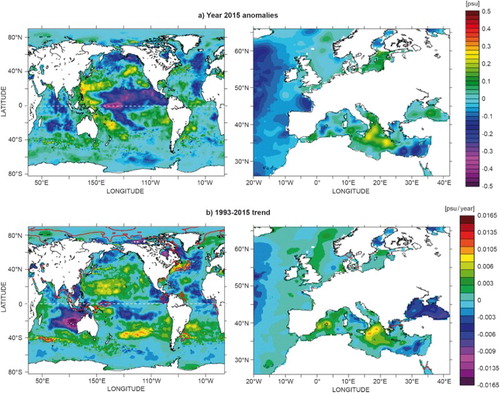
In CMEMS regions (Figure 1), fresh anomalies (−0.2 psu) are found in the North Atlantic Ocean (Figure 8(a) right), associated with the cooling event signal described in previous sections. In the Mediterranean Sea, salinity anomalies are observed in the Ionian basin and fresh anomalies are observed in the Levantine basin, both having similar amplitude of ±0.2 psu. The negative anomalies in the Levantine are related to the surface circulation pattern (see Figure 36(b) of Section 3.1) characterised by a southwestward shift of the Atlantic Ionian Stream, which crosses the channel in a southeasterly direction as one main jet, becoming the Cretan Passage Southern Current and bringing relatively fresh waters to the Levantine and the Aegean. Positive anomalies are instead related to the cyclonic circulation that characterises the Northern Ionian and the Middle and Southern Adriatic.

Additionally, near-surface regional salinity trends during the period 1993–2015 are unevenly distributed (Figure 8(b)). The largest trend of the order of −0.016 psu/yr is the freshening in the Eastern Indian Ocean which seems to be linked to the huge amount of regional rain patterns over and around Australia (Fasullo et al. 2013). Positive salinity trends are also observed in the Northern hemisphere subtropical area which have been reported in previous studies (Boyer et al. 2005; Hosoda et al. 2009; Durack & Wijffels 2010; Good et al. 2014). Positive trends also occur south of the subtropical gyre. Negative trends are located close to the Pacific fresh pool. However, the 1993–2015 trend values are much smaller compared to the ones computed over the past 50 years (Cravatte et al. 2009; Good et al. 2014), which demonstrate the great importance of decadal variability in this region. Formal error adjustment of the least-square fit is maximum in this region with values of 0.001 psu/yr.

These SSS changes have been related to an intensification of the global water cycle (Durack 2015) since the wet regions dominated by strong precipitation become fresher and the dry regions dominated by strong evaporation become saltier. Climate coupled models are also able to reproduce these SSS changes but with lower magnitude of changes and only if anthropogenic CO₂ forcing is included (Terray et al. 2012; Durack et al. 2014). In the Mediterranean Sea, the Ionian basin shows salinity increase of the order of + 0.008 psu/yr. The positive salinity tendency in the Northern Ionian is the effect of the Northern Ionian Reversal (NIR) in 1997 and the successive prevailing of a cyclonic circulation pattern (see Section 3.1).

The 2015 subsurface zonal mean salinity anomalies reveal complex subsurface patterns (Figure 9). While patterns of amplitudes greater than ±0.03 psu are confined to the first 200 m depth in the Pacific Ocean, they extend to 600 m depth in the Atlantic and Indian Oceans and to 900 m depth in the Mediterranean Sea. A positive salinity anomaly is visible in the upper 200–600 m depth layers of the subtropical southern hemisphere ocean and occurs in parallel to strong warming (see Figure 6, Section 1.2) In the Pacific Ocean, freshening of up to −0.2 psu is concentrated in the area of the ITCZ. In the Indian Ocean, upper ocean (< 200 m) freshening patterns ranging between −0.1 and −0.2 psu are observed in the equatorial band and around 20°S of Australia to east of Madagascar. A salinity increase is also manifested in the northern subtropical area, in particular in the Atlantic centred at 200 m depth, in the Pacific from the surface down to 200 m depth and in the Indian Ocean down to 400 m depth with values up to + 0.2 psu. North of this, both North Atlantic and Pacific Oceans show strong freshening between 45°N and 60°N with values up to −0.1 psu and extending down to 500 m depth. In the North Atlantic, the strong freshening is associated with the strong cooling event signal (∼−1°C) described in Sections 1.2 and 4.2. In the North Pacific, it occurs in parallel to a warming patterns of + 0.6°C (see Section 1.2).

Figure 9. Depth/latitude sections of subsurface salinity anomalies in 2015 relative to the climatological period 1993–2014, see text for more details on the data use. Averages are given for (a) the Atlantic Ocean, (b) the Pacific Ocean, (c) the Indian Ocean and (d) the Mediterranean Sea. Units are psu, contour interval is 0.01, except for the two extreme colours.

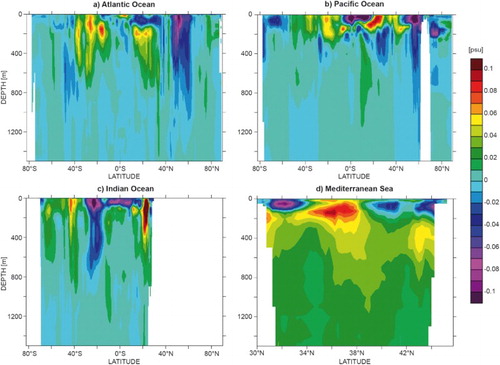
The CMEMS areas of the North Atlantic Ocean, namely IBI and NWS show strong freshening in the year 2015. The Mediterranean Sea (Figure 9(d)), the South Tyrrhenian basin, the Ionian basin and the south Adriatic Sea are much saltier than the long-term mean. The core of the saltier water of up to + 0.25 psu is situated at 150 m depth where the Atlantic Water is located, suggesting a salinification of the Ionian Sea due to the southeastward displacement of the Atlantic Ionian Stream (see Figure 36(b) of Section 3.1). It extends down to 1000 m in the Ionian basin with a value of + 0.04 psu. The salinity signal in fact covers most of the Mediterranean Sea at depth. Fresher waters are found just above in the Levantine basin with a subsurface core of up to −0.2 psu centred at 75 m depth, again explained by the Atlantic Ionian Stream pathway. Slightly fresh waters (∼−0.04 psu) are also found above the salty waters in the western part of the basin (Gulf of Lions, Balearic Sea, northern part of the Tyrrhenian basin).

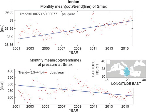
Specific results obtained in the Ionian Sea are now illustrated in order to investigate the temporal evolution of seawater thermohaline properties where transit and redistribution of the major water masses occur. The CMEMS reprocessed regional product¹⁰ based on in situ data has been used for this purpose. The salinity maximum represents the signature of the Levantine Intermediate Water (LIW), which is mainly formed in the Levantine Sea and spreads at an intermediate depth while mixing with other water masses (Menna & Poulain 2010; Pinardi et al. 2015). Along its route towards the Atlantic Ocean, the LIW progressively sinks to 300–350 m in the central basin (Notarstefano & Poulain 2009). The analysis of salinity changes of the LIW core in the Ionian Sea in the last 15 years (2001–2015) is done following the approach of Zu et al. (2014). In particular, the salinity maximum shows (Figure 10 upper panel) a positive trend of the LIW core salinity (the fastest rate is around 0.008 ± 0.0008 psu/yr), with interannual fluctuations ranging between 38.87 psu in 2001 and 2005 and 39.03 psu at the end of 2015. The LIW core depth shows a significant negative trend of −5.5 ± 1.4 dbar/yr (Figure 10, bottom panel). The rising of the LIW depth is well defined between 2009 and 2015 where the mean depth decreased from about 350 to 200 m. This trend could be due to the LIW core temperature increase of about 0.8°C (from about 14.7°C to 15.5°C) in the same period of time (see Section 1.2). The latter affected (reduced) the density of the water mass that varies from about 29.03 kg/m³ in 2001 to 28.97 kg/m³ in 2015. The thermohaline changes of the deep waters are caused by variations in the near-surface and intermediate levels. Hence, it is important to monitor the patterns of salinity (and temperature) changes of a major water mass like the LIW.

Figure 10. Salinity (upper panel) and depth (bottom panel) trends of the LIW core between 2001 and 2015. Locations of Argo profiles in the Ionian Sea are shown in cyan dots (small panel). The identification of the core of the LIW is made possible through a salinity-signature approach (Zu et al. 2014), by looking for the salinity maximal values. See text for more details on data use (only Argo data selected).

1.4. Sea level

Leading authors: Jean-François Legeais, Karina von Schuckmann.

Contributing authors: Quentin Dagneaux, Angélique Melet, Benoît Meyssignac, Antonio Bonaduce, Michaël Ablain and Begoña Pérez Gómez.

Global mean sea level (MSL) rise is one of the most adverse consequences of climate change (e.g. IPCC 2013; von Schuckmann et al. 2016). Note that the sea level is defined as the ECV whereas the sea surface height is the EOV. They are not distinguished in this report, although they have slightly different meaning. The precise monitoring of sea level is crucial to comprehend the socio-economic consequences associated with its contemporary rapid rise and to understand rise due to climate change. Accurate monitoring of this variable is also required to understand the sea level variability and changes over a wide range of temporal and spatial scales, from seasonal to decadal periods and from regional to global scales. Tide gauges have provided sea level measurements for more than a century (e.g. Douglas 1997; Jevrejeva et al. 2008; Woppelmann et al. 2009; IPCC 2013). Since 1993, variations in sea level have been routinely measured by high-precision satellite altimetry (Pujol et al. 2016).

The trend of global MSL during the 1993–2015 period amounts to 3.3 mm/yr (Table 1 and Figure 11; see also Merrifield et al. 2009; IPCC 2013). The uncertainty associated with this trend is±0.5 mm/yr (Ablain et al. 2015). The present-day global MSL rise primarily reflects ocean warming (through thermal expansion of sea water) and ocean mass increase in response to land ice melt. It is essential to distinguish the different contributions to sea level changes (steric signal and ocean mass). The trend of the thermosteric component (0–700 m) amounts to 1.0 mm/yr, which is almost one-third of the total MSL trend (Table 1 and the blue and green curves in Figure 11, left panel). The steric contribution of the deep ocean is expected to be significantly smaller and the associated uncertainty can reach up to 0.7 mm/yr (Llovel et al. 2014; Dieng et al. 2015; Legeais et al. 2016). Significant interannual variations can clearly be distinguished on the global altimeter MSL time series (Figure 11) and contribute to the global MSL trend uncertainty (Cazenave et al. 2014). These variations are mainly attributed to the ENSO (Ablain et al. 2016) and illustrate the impacts of the 1997 and 2015 (+ 0.5 cm) El Niño events (Nerem et al. 2010; Capotondi et al. 2015) and the extraordinary accumulation of rainfall over land (Boening et al. 2012) (−0.6 cm) following the 2011 La Niña event (Cazenave & Remy 2011; Dieng et al. 2014).

Figure 11. Temporal evolution of globally (left) and regionally (right) averaged daily MSL without annual and semi-annual signals (blue), 9-month low-pass filtered MSL (red) and annual mean thermosteric sea level (0–700 m) (green, uncertainty estimation method after von Schuckmann et al. 2009) anomalies relative to the 1993–2014 mean. In the right panel an arbitrary offset has been introduced for more clarity. From top to bottom, the regions are NW Shelf, IBI, Med. Sea and Black Sea. No thermosteric contribution is shown for the Black Sea due to the scarcity of the in situ temperature observations in this region. In this figure, no Glacial Isostatic Adjustment (GIA) correction has been applied to the total MSL whereas a correction for the glacial isostatic adjustment was added for the MSL trends in Table 1. See Table 1 for the definition of the dataset.

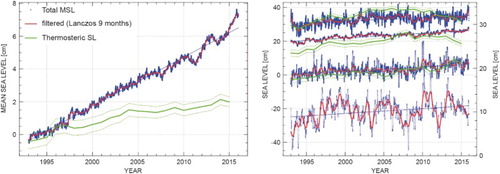
Table 1. Mean sea level trends during January 1993–December 2015 for the global ocean and different CMEMS regions for the total altimeter sea level (corrected from the Glacial Isostatic Adjustment – GIA, e.g. Tamisiea, 2011) and the thermosteric sea level. Associated uncertainties at global and regional scales are derived from Ablain et al. (2015), Prandi et al. (2016) and von Schuckmann et al. (2009), respectively. Results are based on the CMEMS reprocessed altimeter sea level product^a for total sea level. Thermosteric sea level (0–700 m) is derived from the CMEMS reprocessed product of global in-situ observations^b for the 1993–2014 period, and extended using the CMEMS real-time product^c. A mean salinity climatology over the period 1993–2014 is used from the CMEMS reprocessed product for the evaluation of thermosteric sea level. The thermosteric anomalies are derived relative to the 1993–2014 period and relative to the 1993–2012 period for total sea level.

Regions	Mean sea level trend (1993–2015) (mm/yr)
	Total (GIA corrected)	Thermosteric
Global ocean	3.3 ± 0.5	1.0 ± 0.1
NW shelf	2.6 ± 0.8	1.1 ± 0.3
IBI	3.1 ± 0.5	1.5 ± 0.2
Med. Sea	2.9 ± 0.9	1.5 ± 0.2
Black sea	3.2 ± 2.5	–
Baltic sea	–	–

^aSEALEVEL_GLO_SLA_MAP_L4_REP_OBSERVATIONS_008_027 (PUM: http://marine.copernicus.eu/documents/PUM/CMEMS-SL-PUM-008-017-033.pdf; QUID: http://marine.copernicus.eu/documents/QUID/CMEMS-SL-QUID-008-017-037.pdf).

^bINSITU_GLO_TS_OA_REP_OBSERVATIONS_013_002_b (PUM: http://marine.copernicus.eu/documents/PUM/CMEMS-INS-PUM-013-002-ab.pdf; QUID http://marine.copernicus.eu/documents/QUID/CMEMS-INS-QUID-013-002b.pdf).

^cINSITU_GLO_TS_OA_NRT_OBSERVATIONS_013_002_a (PUM: http://marine.copernicus.eu/documents/PUM/CMEMS-INS-PUM-013-002-ab.pdf).

In the CMEMS regions, the total MSL trends observed in the NWS and IBI regions as well as in the Mediterranean Sea are positive and relatively close to each other. About half of these trends are attributed to the thermosteric contribution to sea level (Table 1). Following Prandi et al. (2016), at basin scale, two contributors to the altimeter trend uncertainty can be distinguished. The altimetry errors are one of the contributors. They can be related to the reduced quality of the altimeter sea level estimation in coastal areas and to the greater error of some geophysical altimeter corrections (ocean tide, inverse barometer and dynamic atmospheric corrections). For these reasons, the MSL time series is not provided for the Baltic Sea. The second contributor is related to the large internal variability of the observed ocean (and the fact that the associated trend may vary with the length of the record). The local variability is generated by regional changes in winds, pressure and ocean currents which averaged out at global scale (e.g. Stammer et al. 2013) but this can significantly contribute to the MSL uncertainty at basin scale. Both altimetry errors and internal variability explain why slightly greater interannual variations are found in the Mediterranean and Black Seas (semi-enclosed basins) than in the NWS and IBI regions (larger, deeper and open ocean areas) (see Figure 11, right panel). The uncertainties indicated in Table 1 for the CMEMS regions include both contributions.

The regional sea level trends during 1993–2015 are generally considerably larger than those observed at the global scale (values range spatially between −5 and + 5 mm/yr around the 3 mm/yr global estimate). This is explained by the large local variability mentioned above. The altimeter MSL trends during 1993–2015 exhibit large-scale variations with amplitudes reaching up to + 8 mm/yr in regions such as the western Tropical Pacific Ocean and the Southern Ocean (Figure 12, top left). The regional sea level trend uncertainty is of the order of 2–3 mm/yr with values as low as 0.5 mm/yr or as high as 5.0 mm/yr depending on the regions (Ablain et al. 2015; Prandi et al. 2016). In the European region, relatively homogeneous trends can be found in the NWS and IBI regions (∼2–3 mm/yr) (Figure 12, top right). In the open ocean, these trends are mainly of thermosteric origin (Figure 12, bottom right). Larger total sea level trends are found in the Baltic Sea (up to 6.0 mm/yr). However, as mentioned above, less confidence is attributed to the sea level estimation in this region. In the Mediterranean Sea, positive trends are observed in the Adriatic Sea, in the Aegean Sea and in most of the Eastern basin, especially where recurrent gyres and eddies are found. Negative trends are detected in the Levantine basin associated with the Ierapetra gyre and in the Ionian Sea as a consequence of a large change in the circulation (the Eastern Mediterranean transient) which has been observed in this basin since the beginning of the 1990s (Demirov & Pinardi 2002; Pinardi et al. 2015; Bonaduce et al. 2016).

Figure 12. Spatial distribution of the total (top) and thermosteric (0–700 m) (bottom) sea level trends during 1993 – December 2015 (in mm/yr) over the global ocean (left) and the European Seas (right). No GIA correction has been applied on the altimeter data. See Table 1 for the definition of the dataset.

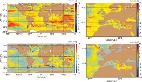
Regional thermosteric sea level trends resulting from non-uniform ocean thermal expansion (Figure 12, bottom left) are mostly related to changes in ocean circulations, atmospheric forcing and the inferred distribution of heat (e.g. Wunsch et al. 2007; Lombard et al. 2009; Levitus et al. 2012; Fukumori & Wang 2013; Stammer et al. 2013; Forget & Ponte 2015). The largest regional variations in sea level trends – mainly of thermosteric origin – are observed in the Pacific Ocean and are in response to increased easterlies over the Equatorial Pacific during the last two decades associated with the decreasing Interdecadal Pacific Oscillation (IPO)/Pacific Decadal Oscillation (e.g. McGregor et al. 2012; Merrifield et al. 2012; Palanisamy et al. 2014; Han et al. 2010; Rietbroek et al. 2016). A positive thermosteric sea level trend is observed in almost all CMEMS regions (Figure 12, bottom right), in particular in the Eastern Mediterranean Sea basin. Note that evaporation and precipitation can also play an important role in regional sea level trends locally (e.g. the Atlantic) (e.g. Durack & Wijffels 2010).

The sea level anomaly (SLA) field for 2015 is dominated by the dipole (±) observed in the Equatorial Pacific Ocean associated with the El Niño event (Schiermeier 2015) with an anomalously high sea level in the Eastern Equatorial Pacific, and an anomalously low sea level in the western basin (Figure 13, left). In the North Atlantic, an anomalous low sea level pattern occurs in the same area where the recent North Atlantic cooling event is reported (see Section 4.2). In the Baltic Sea, the observed positive anomaly (Figure 13, right) is related to a major inflow event that took place in late 2014 to early 2015 in connection with westerly winds and low air pressure (Mohrholz et al. 2015). In the Mediterranean Sea, a lower sea level has been observed in 2015 compared to its climatologic mean over the entire basin. This is not observed in Figure 11 (right) where the trend is included. Such a basin-wide oscillation can be related to a basin adjustment process responding to changes in mass flux through the Strait of Gibraltar forced by the wind (Fukumori et al. 2007) but also to the interannual variability observed in this region (Pinardi & Masetti 2000; see also Sections 2.4 and 3.1).

Figure 13. Global (left) and regional (right) spatial variability of the difference between the detrended altimeter MSL during [2015] and [1993–2014].

1.5. Ocean colour – Chlorophyll-a

Leading authors: Shubha Sathyendranath and Robert Brewin.

Contributing authors: Cosimo Solidoro, Marie-Fanny Racault and Dionysios Raitsos.

Phytoplankton are recognised as an Essential Climate Variable (ECV) in the implementation plan of the Global Climate Observing System (GCOS 2010). They are microscopic, single-celled, floating, marine organisms capable of photosynthesis: they take up dissolved carbon dioxide in the water in the presence of sunlight to produce organic material. Chlorophyll-a is a measure of phytoplankton concentration. All higher pelagic organisms, including fish, depend on phytoplankton for their nutrition. Phytoplankton are therefore the primary producers of the sea. They are present everywhere in the sunlit layers of the ocean in varying concentrations, and are collectively responsible for a net primary production of some 50 pg of carbon per year, globally (Longhurst et al. 1995). This amount is roughly equivalent to the net primary production by all terrestrial plants. Primary production modulates the total concentration of dissolved carbon dioxide (CO₂) in the ocean, and hence influences the transfer of CO₂ between the atmosphere and the ocean. Some phytoplankton sinks out of the surface layer, thus exporting carbon to the deep ocean.

It is estimated that some 48% of the anthropogenic CO₂ emitted into the atmosphere now resides in the ocean (Sabine et al. 2004). The dissolution of this CO₂ in the ocean has changed the oceanic alkalinity and pH – referred to as ocean acidification – whose impact on the marine biota is yet to be fully understood. Some phytoplankton types, known as coccolithophores, produce calcium carbonate (CaCO₃) liths or plates that cover their body. Blooms of coccolithophores have been observed by satellites that cover millions of squared kilometres of the surface ocean, but only under conditions favourable for formation of such blooms. The production of CaCO₃ particulates by phytoplankton lowers the pH of the water, which favours outgassing of CO₂. On the other hand, the carbon that is embedded in the CaCO₃ is likely to sink into the deep ocean.

Phytoplankton consists of thousands of species belonging to different genera, and come in many shapes and sizes ranging from less than one micron to over a hundred microns. All phytoplankton photosynthesise but, in addition, they also contribute significantly to other major biogeochemical cycles, although these functions may vary with the phytoplankton type involved (Nair et al. 2008; IOCCG 2014). The role of coccolithophores in formation of calcium carbonate has already been discussed. Diatoms incorporate silica into their frustules (a type of exoskeleton), impacting the export and cycling of silica. Cyanobacteria, or blue-green algae, are capable of taking up dissolved nitrogen in the water. Some types of phytoplankton are also producers of volatile organic compounds, such as dimethylsulphoniopropionate (DMSP), a precursor of dimethyl sulphide. The broad spectrum of sizes that phytoplankton occupy also contributes to their functional diversity, since many phytoplankton functions, such as respiration, light absorption, sinking and nutrient uptake are size-dependent.

Phytoplankton represent a diverse community with multiple functions. The first step in photosynthesis is the capture of solar energy through a suite of phytoplankton pigments. The most important, and the most ubiquitous, of all phytoplankton pigments is chlorophyll-a. The concentration of chlorophyll-a is a fundamental biological property because of the central role it plays in photosynthesis, and it is therefore important to monitor its variability. In fact, chlorophyll concentration is amenable to remote sensing because of its optical properties: chlorophyll-a and auxiliary pigments absorb light most efficiently in the blue part of the spectrum, such that the colour of the water changes progressively from blue to green with the increase in chlorophyll concentration. This change in colour can be detected using visible spectral radiometers in space, recording radiances at the top of the atmosphere in a number of spectral wavebands in the visible domain. These signals can be converted using appropriate algorithms into quantitative estimates of chlorophyll concentrations in the surface layers of the ocean (Figure 14). Using such algorithms, the distribution of chlorophyll concentration in the surface layers of the global oceans on a daily basis and at high spatial resolution of better than 1 km can be mapped. However, these empirical algorithms require regional tuning as the relationships between chlorophyll and other optically active components (e.g. the amount of coloured dissolved organic matter in the water) that impact radiances observed by radiometers vary regionally (Figure 14). Once chlorophyll is computed, the daily information can then be used to produce climatologies at various time scales: weekly, monthly, annual or multi-year. For example, see Figure 15, which shows a multi-year climatology computed using the Ocean Colour – Climate Change Initiative (OC-CCI) products (version 3.0, OC-CCI is a European Space Agency initiative), which is also a CMEMS reprocessed product.¹¹ Being small, phytoplankton have high metabolic rates, and respond rapidly to changes in environmental conditions (notably, light, nutrient supply, mixing and temperature). Since phytoplankton represent the first link between the marine biota and their energy source (sunlight), it is to be expected that changes in the marine ecosystems would first manifest themselves through changes in the phytoplankton concentration, their species composition and their phenology (timings of important events in the phytoplankton calendar). It is, therefore, of utmost importance to monitor phytoplankton concentrations at multiple time and space scales. Since environmental variability in the oceans is known to occur over long time scales including decadal-scale oscillations, multi-decadal observations of the marine ecosystem in general, and phytoplankton in particular, are needed in order to isolate any climate signal from natural variability.

Figure 14. Relationship between chlorophyll-a concentration and the ratio of blue to green remote-sensing reflectance (Rrs), with the maximum Rrs in blue bands (443–510 nm) divided by that at 555 nm (green bands). In situ chlorophyll-a data (coloured-squares, coloured according to the number of samples, N) were collected as part of the OC-CCI project (Valente et al. 2016) and these were matched to Rrs data from the OC-CCI project (version 2.0). The global algorithm is that of O’Reilly et al. (2000); Med (Mediterranean) is that of Volpe et al. (2007); Baltic is from Pitarch et al. (2016); and the Arctic is that of Cota et al. (2004). Note that the global algorithms are designed for open-ocean (so-called Case 1) waters, and regional algorithms tend to diverge most from global algorithms in coastal (Case 2) waters. Note that none of the algorithms shown in the figure have been re-tuned using the OC-CCI in situ data shown in the figure.

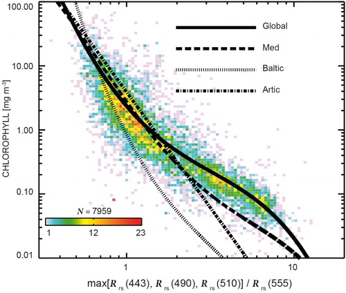
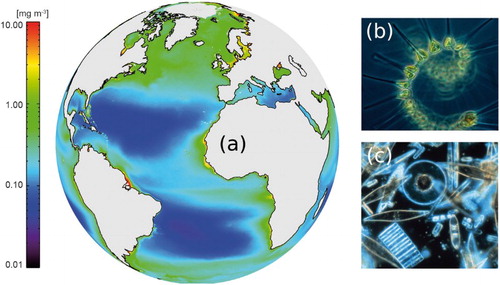
Figure 15 (a) Climatology of chlorophyll concentration in the Atlantic and Artic Oceans. See text for more details on data use. (b) Microscopic image of phytoplankton (credit NOAA MESA Project, source http://www.photolib.noaa.gov/bigs/fish1880.jpg). (c) Assorted phytoplankton (diatoms) living between crystals of annual sea ice in Antarctica (credit NSF Polar Programs, source http://www.photolib.noaa.gov/htmls/corp2365.htm).

It has been shown that regional-scale interannual variations in phytoplankton seasonality in the Pacific Ocean (Behrenfeld et al. 2006; Racault et al. 2012) and in the Red Sea (Raitsos et al. 2015) can be associated with the ENSO and Brewin et al. (2012) have shown that interannual variations in phytoplankton distribution in the Indian Ocean is related to the Indian Ocean Dipole (IOD). Climate indices may represent regional ocean physics and broader climate oscillations that ultimately can be positively (i.e. Red Sea) or inversely related (i.e. Pacific and Indian Oceans) to variations in phytoplankton. The type of ENSO can also impact the phytoplankton chlorophyll concentration at regional scales (e.g. in the Tropical Pacific, see Radenac et al. 2012). Figure 16 shows the links between interannual variations in phytoplankton chlorophyll concentration in the Pacific Ocean and the Indian Ocean, and their correspondence with ENSO and the IOD, respectively. The correspondence is remarkable, and the regional differences in the time series of ocean colour data are very clear. These regional responses to climate variability give us important clues on how phytoplankton might respond to long-term climate changes. The 2015–2016 ENSO event was the strongest observed since 1997, and in parallel a large reduction in phytoplankton chlorophyll concentration occurs in the Equatorial Pacific Ocean (Figure 17), which has not been seen since 1997 (Figure 16).

Figure 16. Relationship between chlorophyll-a and the ENSO and IOD climate modes. Note that the scale of chlorophyll anomalies is inverted. Chlorophyll images are from an annual climatology (see text on more details for data use). The monthly multivariate ENSO Index (MEI) was downloaded from the NOAA website (http://www.esrl.noaa.gov/) and the IOD Mode Index (IOD) was taken from the JAMSTEC website (http://www.jamstec.go.jp). Weekly values of the IOD from 1981 to the present were derived from NOAA OISST version 2, and were smoothed with a 12-point (3-month) running mean. Monthly chlorophyll data were taken from OC-CCI/CMEMS (see text). The time series of chlorophyll anomalies for the IOD represent the difference in chlorophyll anomaly between the two boxes in the Indian Ocean (see Brewin et al. 2012).

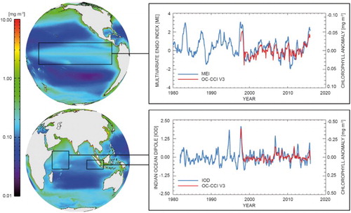
Figure 17. Annual anomalies in chlorophyll from 1998 to 2015 (see text for details on data use). Anomalies were computed by calculating annual averages (from monthly composites) then subtracting the average of all 18 years from each year. Computations were done in log10-space, considering the typical distribution of chlorophyll concentration (Campbell 1995).

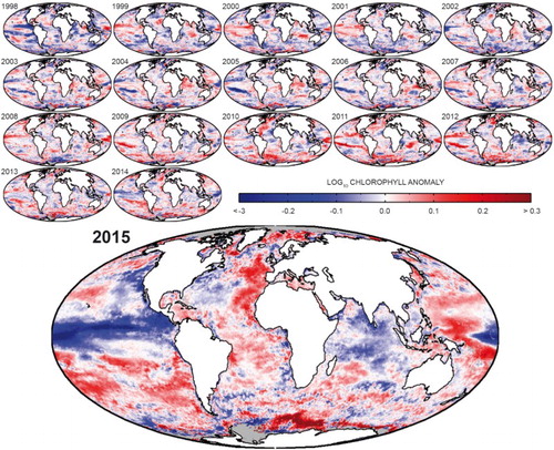
In the tropical regions, large reductions in chlorophyll concentration were observed in the Indian Ocean, Equatorial Pacific, North-Eastern Pacific and Western North Atlantic, in 2015 (Figure 17). These reductions are associated with positive anomalies in SST and sea level (see Sections 1.2 and 1.4) which is indicative of enhanced stratification. In low latitude regions, where light is plentiful, phytoplankton in the surface layer are thought to be limited by nutrient availability (Doney 2006). Enhanced stratification limits the vertical transfer of nutrients and can significantly reduce chlorophyll concentration in the surface layer. In contrast, higher chlorophyll concentrations were observed in the North-Eastern and Tropical Atlantic, most of the Mediterranean, western Equatorial Pacific, South Pacific and western North Pacific. In lower latitude regions (< 40°), increases in chlorophyll are generally consistent with slightly lower SST and sea level anomalies (see Sections 1.2 and 1.4), indicative of enhanced mixing and increased vertical nutrient transport. Note, however, that the increase in chlorophyll in the Mediterranean appears to be associated with an increase in SST (see Figure 3b).

Remote sensing of phytoplankton through ocean colour must form a part of an observational strategy, because of the global reach of satellite observations, and because of the high repeat cycle (of about a day) that is possible. The importance of being able to make all these observations using a common approach, and using the same instrument, cannot be overstated.

1.6. Currents

Leading authors: Marie Drévillon, Hélène Etienne.

Contributing authors: Joaquin Tintoré, Stéphanie Guinehut, Eric Greiner, Yann Drillet and Sandrine Mulet.

Ocean currents are essential for understanding heat exchanges between the ocean and atmosphere. These heat exchanges through local and global ocean currents affect the regulation of local weather conditions and temperature extremes, and the stabilisation of global climate patterns. Currents also transport plankton, fish, momentum and chemicals such as salts, oxygen and CO₂, and are a significant component of the global biogeochemical and hydrological cycles. Knowledge of ocean currents is also extremely important for marine operations involving navigation, search and rescue at sea, and the dispersal of pollutants.

The ocean has an interconnected current, or circulation, system powered by winds, tides, solar energy, water density differences and steered by the Earth’s rotation (Coriolis Effect) and by tides, waves and bathymetry. Meridional currents transporting stored solar heat from the tropics to the polar regions are a critical element of the Earth’s climate system as they contribute to balancing the Earth’s global energy budget. Deep ocean currents are density-driven and contribute to the Meridional Overturning Circulation. Surface currents interact with the atmosphere and respond to wind changes: in the gyres and boundary currents, in the Antarctic Circumpolar Current (ACC) and in the tropics strong currents are connected with the trade winds.

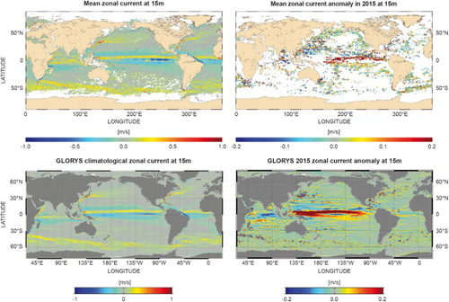
The large-scale and interannual fluctuations of surface currents are well captured by zonal current fluctuations, as seen for instance in Blunden and Arndt (2016). Two different CMEMS products were used for the analysis, i.e. the CMEMS reprocessed global product on ocean surface currents from in situ observations¹² and the CMEMS global reanalysis product GLORYS (GLobal Ocean ReanalYsis and Simulation).¹³ The mean surface zonal currents are displayed on a climatology obtained from drifters (Figure 18(a)) and in one obtained with a 3D ocean reanalysis on the same 1993–2014 period (Figure 18(c)). The two climatologies are complementary as they are produced and validated independently, one from in situ observations only, and the other from a 3D multivariate ocean reanalysis, which does not assimilate drifter measurements. The main surface current features that are present on average over the period in the mid-latitudes are the eastward-flowing part of the western boundary currents and the ACC. In the tropics, the Tropical Pacific South Equatorial Current (SEC) and the North Brazil current in the Tropical Atlantic reach average westward velocities of the order of 1 m/s. Eastward North Equatorial Counter Currents (NECC) are captured in the Atlantic and Pacific, while in the Indian Ocean the signature of the Somali Current, the Equatorial Counter Current and of the North and South Equatorial Currents can be seen.

Figure 18. 1993–2014 average near surface (15 m) zonal current (a) and zonal current anomaly in 2015 (relative to the 1993–2014 mean) (b) computed from in situ observations (see text for more details on data use). (c) and (d) identical to (a) and (b) but computed from GLORYS (see text for more details). Spurious strong currents are diagnosed by the reanalysis off New Guinea, which is a known sea surface height bias of the Mercator Ocean monitoring system (Lellouche et al. 2013). Positive values indicate eastward, negative values westward currents.

Surface currents experience intrinsic oceanic interannual variability (Penduff et al. 2011; Sérazin et al. 2015) and respond at several time scales to large-scale variability patterns in the atmosphere such as the North Atlantic Oscillation (Frankignoul et al. 2001).

1.6.1. Currents in the Tropical Pacific

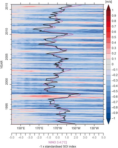
The annual average surface Tropical Pacific current system climatology is displayed in Figure 19(a). It corresponds well to the description obtained from drifters given by Reverdin et al. (1994) with the westward-flowing NECC between 4°N and 8°N, in between the eastward-flowing NEC north of 8°N, and SEC south of 4°N, which splits into two branches on each side of the equator. These two branches are separated at subsurface by the westward-flowing equatorial under current centred around 150 m underneath the Equator, while the NECC is deeper and flows westward from the surface to around 400 m (Godfrey et al. 2001). The Tropical Pacific current variability has been extensively studied as it is constitutive of ENSO variability (see, for instance, Mcphaden et al. 1998; Delcroix et al. 2000; Meinen and Mcphaden 2001). In 2015 the El Niño event (see also Section 4.1) had a strong signature on surface currents in the Tropical Pacific. The Tropical Pacific current system experienced a large positive eastward anomaly in 2015, associated with the slowing down of the trade winds, eastward propagating downwelling Kelvin waves and associated transfer of heat from the western Tropical Pacific Ocean warm pool towards the Central and Eastern Tropical Pacific as described for previous El Niño events for instance in Meinen and Mcphaden (2001) or Delcroix et al. (2000). This resulted in a slowing down of the westward, northern and southern branches of the SEC, and in the strengthening of the NECC as shown by Figure 19(b). As illustrated in Figure 19(c), this strong eastward current anomaly in the Tropical Pacific was even larger during the El Niño event of 1997/1998. This is confirmed by the longitude time diagram of the zonal velocity in Figure 20. While the correlation between average eastward-flowing surface currents in the Tropical Pacific and ENSO indices is very clear, the amplitude of the change in surface currents and their spatial features (as shown in Figure 19) are very different between events. Climate change and decadal variability involve changes in ocean–atmosphere coupling mechanisms that may explain some of these differences (Mcphaden 2015). Note that El Niño also induces a westward equatorial current in the Indian basin, which is seen clearly in 3D ocean analyses (Figure 18(d)) and is only guessed in the drifters’ measurements (Figure 18(b)) due to the lack of observations.

Figure 19 (a): total velocity at 15 m (m/s) climatology 1993–2014, and (b) the same quantity in 2015 computed from GLORYS (see text for more details), and c) for the year 1997. The colours stand for the velocity (m/s) and the arrows indicate the direction of the current.

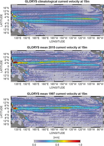
Figure 20. Latitude time diagram of the zonal current anomaly (m/s) in the Tropical Pacific Ocean (25°S–25°N), with respect to the 1993–2014 climatology, and computed from the in situ current observations (see text for more details). Positive values indicate eastward, negative values westward currents. The pink line indicates the NINO3.4 index from GLORYS, and the black line is the standardised Southern Oscillation Index (https://www.ncdc.noaa.gov/teleconnections/enso/indicators/soi/).

1.6.2. Variability of currents at mid-latitude

At mid-latitudes in 2015, zonal current anomalies do not display large-scale features but substantial anomalies are seen in the western boundary currents, Kuroshio and Gulf Stream, including the loop current in the Gulf of Mexico, as well as in the ACC (Figure 18(d)). The Gulf Stream and Kuroshio currents are major actors in the transfer of heat from the tropics to the North Atlantic and North Pacific, respectively, and to the Arctic region. Part of their interannual variability comes from large eddies or meanders, and part of it can be related to low-frequency variability of the climate system. Variability at interannual to decadal timescale can also be understood as ‘regime shifts’ related to climate variability modes such as the North Atlantic Oscillation (NAO) or the PDO, also impacting the ocean ecosystems (Overland et al. 2008). One way to characterise large-scale surface current features which co-vary in time is to perform an empirical orthogonal functions (EOF) analysis of surface currents. The spatio-temporal modes obtained from the GLORYS reanalysis zonal surface currents displayed in Figures 21 and 22 are the first modes of variability in the Gulf Stream (Figure 21) and Kuroshio (Figure 22) regions. These modes are robust in the sense that they are also found when the same analysis is performed on near-surface currents deduced from satellite observations (from altimetry plus Ekman, not shown). These modes reflect changes in the mean path position and intensity of the currents related to large-scale variability changes of SSH such as shown for instance in Tagushi et al. (2007), or SST in Overland et al. (2008).

Figure 21 (a) First low-frequency (all inputs are filtered with 4 years running window) spatio-temporal variability mode of 15 m zonal current (m/s) from EOF analysis of GLORYS (1993–2015, see text for more details). The colour shading shows the adimensional spatial pattern of the mode, and a white box (hereafter called index box) is drawn on a high variability region inside this pattern. The time series of amplitude (m/s) of the mode is shown in the bottom panel: black line: zonal current anomaly (m/s) the corresponding mode; blue line: zonal current average from GLORYS in the index box, thick red line: median of zonal velocity (m/s) from drifter in situ observations (see text for more details) in the index box, thin red lines: interval of confidence for the thick red line defined as 40th and 60th percentiles. The median of all drifters in the index box and on the whole period was retrieved to time varying median and percentiles, in order to build monthly anomaly ‘distributions’ within a 4-year running window. The correlation between the thick blue and red lines is indicated along the x-axis.

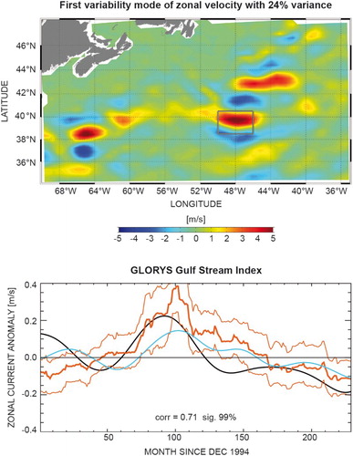
Figure 22. As in Figure 21, but for the first mode of variability of zonal current in the Kuroshio region.

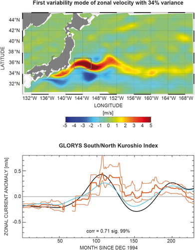
From the spatial patterns of the modes, subregions experiencing the strongest signals were located (boxes in Figures 21(a) and 22(a)), and simple zonal velocity statistics (average, median and 40th and 60th percentiles) were computed in these boxes from GLORYS and from drifter observations (Figure 21(b) and 22(b), see endnotes 12 and 13). Low-frequency variations are well captured by these simple indices, as they are well correlated with the principal components, especially in the Kuroshio for both modes 1 and 2 (not shown). Note that indices derived from drifters’ measurements, despite differences in representativeness related to sampling issues (not shown), are significantly correlated with indices from the GLORYS global reanalysis. Again, two independent estimates give a consistent view of the ocean variability over the past decades, and can be used to further assess the physical mechanisms related to these changes. Ocean Monitoring Indices for surface currents will be derived from this preliminary exploration, and the study could be extended to the ACC in future issues of this report.

1.7. Sea ice

Leading authors: Annette Samuelsen, Lars-Anders Breivik, Roshin P. Raj, Gilles Garric, Lars Axell.

Contributing author: Einar Olason.

Sea ice acts as a physical barrier and controls the exchange of heat, light and wind power between the ocean and atmosphere in polar regions. Sea ice affects the climate in the polar regions and the Baltic and likely also at lower latitudes (Gao et al. 2014); at the same time Arctic sea ice is one of the most visible indicators of our changing climate. Presently, it is observed that the sea ice in the Arctic is steadily shrinking and thinning (Stroeve et al. 2005; Kwok & Rothrock 2009; Laxon et al. 2013). With thinner ice, the action of winds, currents and waves acts to break ice into smaller pieces more effectively, potentially accelerating melting. In the Antarctic, a small increase in sea ice extent has been observed (Parkinson & Cavalieri 2012).

Sea ice presents a hazard to shipping and other marine operations and the monitoring and forecasting of sea ice is, therefore, important to reduce risks for these activities. For example, the ice extent is an important socio-economic factor for the countries surrounding the Baltic Sea, and may also become so for increased shipping in the Arctic in the future. Sea ice also affects the marine ecosystem, and changes in ice cover will likely shift the ratio between ice algae and open ocean primary production (Wassmann & Reigstad 2011). Many marine organisms in the polar regions also rely on sea ice as part of their life cycle and changes in the thickness and extent of the sea ice will affect several aspects of the polar ecosystems (Meier et al. 2014).

Sea ice can be characterised by its extent (here defined as an area with an ice concentration above 15%), concentration, thickness and volume. For the last decades these characteristics have been monitored by satellites and estimated by numerical models, while the record can be extended back hundreds of years by use of proxies. For sea ice extent, there exists a satellite record from 1979 until today and in recent years unprecedented lows in the Arctic sea ice extent were observed as in 2007 followed by a new minimum in 2012 (Parkinson & Comiso 2013). The Baltic Sea, which only has a seasonal ice cover, saw a minimum in its annual maximum ice extent in March 2008, and an even smaller maximum extent in 2015.

The spatial extent of the sea ice in the Arctic has been analysed by using the CMEMS global reanalysis GLORYS (see Section 1.6, endnote 13), the CMEMS regional reanalysis product¹⁴ combined with the CMEMS regional forecasting product¹⁵ (Figure 23) and from the CMEMS reprocessed regional product¹⁶ for the Arctic (Figure 24). The results show that the spatial extent of the sea ice in the Arctic varies by more than 50% between summer and winter (Figures 23 and 24) and reaches its yearly maximum between February and April. In 2015, the sea ice winter maximum extent was significantly below the 1993–2014 baseline, and the maximum value was reached relatively early. In the Arctic, the minimum ice extent is normally reached around mid-September, and a low winter maximum points towards a low summer minimum. However, the situation in September depends strongly on the summer weather (atmosphere and ocean), and as seen from Figure 24(a) the 2015 sea ice minimum was low, but within one standard deviation of the 1993–2014 period mean. The September sea ice extent was less than the long-term mean along the Russian and western North American coast, while ice remained to the north of Greenland and in Eastern Canada. This is the same pattern that was seen during the summer minimum of 2012 (Figure 23(a)). The 1993–2015 dataset confirms the decreasing trend of 76,300 km²/yr of Arctic sea ice extent (Figure 24(b)). Both in the Arctic and the Baltic, the sea ice in 2015 was less than the mean (Figures 24 and 25). In the Baltic, the sea ice extent in 2015 was mostly more than one (up to two) standard deviation lower than the mean.

Figure 23. Map of the border of the March and September sea ice extent in the Arctic (left) and Antarctic (right), respectively. The sea ice extent is from the CMEMS global reanalysis product GLORYS, except for the Arctic September sea ice extent which is from the CMEMS regional reanalysis product for the Arctic and the Arctic forecasting product (see text for more details).

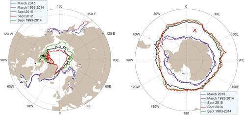
Figure 24. (a) Arctic seasonal cycle of the sea ice extent; long-term mean (blue line) and standard deviation (blue shading), 2012 (green line) and 2015 (red line). (b) Time series for Arctic sea ice extent anomaly (with respect to the mean seasonal cycle). Both plots are based on the CMEMS reprocessed regional product, see text for more details on data use.

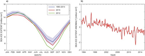
Figure 25 (a) Baltic seasonal cycle of the sea ice extent; long-term mean (blue line), standard deviation (blue shading) and 2015 (red line). (b) Time series for Baltic sea ice extent from 1993 to 2015. Both plots are based on operational ice charts from SMHI.

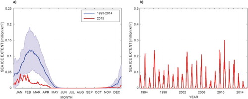
Since the Arctic is a semi-enclosed ocean, almost completely surrounded by land while Antarctica is a land mass surrounded by an ocean, sea ice in the Antarctic differs from that in the Arctic in many ways. The Southern Ocean is dominated by the ACC and circumpolar winds. This causes ice formed in the Antarctic to drift primarily around and away from the Antarctic continent and north into the Southern Ocean. Compared to the closed Arctic Basin, ice in the Antarctic therefore moves more freely, resulting in higher drift speeds and fewer ridges. Also, because there is no land boundary to the north of Antarctica, the sea ice is free to float northward into warmer waters where it eventually melts. As a result, almost all of the sea ice that forms during the Antarctic winter melts during the summer, and the Antarctic is virtually free of thick multi-year sea ice. The amplitude of the seasonal cycle in the Antarctic is also twice that of its boreal counterpart. During the winter, up to 20 million square kilometres of ocean is covered by sea ice, but by the end of summer, only about 3 million square kilometres of sea ice remain. As shown in the CMEMS global reanalysis GLORYS, the South reaches its summer minimum in late February, while the North reaches its summer minimum in September. March is shown for both hemispheres for consistency (Figures 23 and 26).

Figure 26 (a) Antarctic seasonal cycle of the sea ice extent; long-term mean (blue line) and standard deviation (blue shading), and 2015 (red line). (b) Time series for Antarctic sea ice extent anomaly. Both plots are based on the CMEMS global reanalysis product GLORYS (see text for more details).

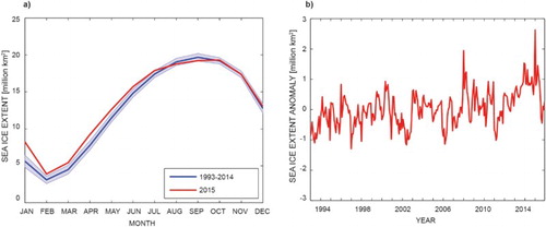
Figure 26(a) shows a modest year-to-year variability in the Antarctic compared to the seasonal cycle. While Arctic sea ice has set record lows, Antarctic sea ice has set record highs and has been increasing (Parkinson & Cavalieri 2012). Antarctic sea ice expanded to 20.826 million km² in September 2014. It was the highest Antarctic sea ice extent in the satellite record, surpassing record-high extents set during the previous two years. The 2015 Antarctic sea ice maximum, however, was closer to the long-term average. The overall trend is positive at 44,900 km²/yr.

An important question in relation to sea ice is not only its extent, but also its volume and thickness. Presently, sea ice volume estimates from satellites are associated with large uncertainties (Zygmuntowska et al. 2014). Consequently, modelled sea ice volume is poorly validated and ice thickness observations are seldom assimilated in the ocean reanalysis products. With ongoing improvements in both remote-sensing techniques and modelling it is hoped that the variability and trend of sea ice volume will be covered in future versions of this report. Sea ice volume also relates to freshwater storage (Giles et al. 2012; Rabe et al. 2014) and to estimate changes in freshwater storage requires knowledge of both sea ice volume and drift. While sea ice drift is observed and assimilated in the models, the uncertainty with regards to freshwater export is still present because of its dependency on ice thickness.

Chapter 2: Large-scale changes

Monitoring the state of the ocean is not only a question of having reliable observations and model products at hand. It also requires transforming these data into (useful) information. As stated in the introduction, there is a growing need for an ocean monitoring capability that captures the main ocean variability features and also aims to measure the direct impact of ocean changes on society. The purpose of this chapter is to deliver insight on large-scale changes of the physical state of the ocean which are known to contribute fundamentally to the role of the ocean in global and regional changes of the Earth’s climate system. This first report will focus on Ocean Heat Content at global and regional scales, ocean volume transport reflecting changes of the Atlantic meridional overturning circulation (AMOC), ocean transport responsible for the redistribution of ocean mass and heat (energy) in the global ocean, and a global and regional view on mesoscale activity known to influence the large-scale ocean circulation at the surface and in the deep ocean. These components are discussed over the 1993–2015 time window with regional information delivered for different CMEMS regions (Figure 1, introduction) and for key choke points (Section 2.2). With the development of the CMEMS OSR activity, further key processes and mechanisms will be addressed in the future.

2.1. Ocean heat content

Leading authors: Karina von Schuckmann, Magdalena Balmaseda, Simona Simoncelli.

Contributing authors: Mathieu Hamon, Tanguy Szekely.

The only practical way to monitor climate change across time scales is to continually assess the energy, mainly in the form of heat, in the climate system (Hansen et al. 2011). Quantifying these exchanges, and in particular how much heat has resulted from human activities, and how it affects the climate system is one of the key challenges faced by the climate research community (IPCC 2013). A reliable estimate of the state of the Earth’s climate is most robustly determined through taking an inventory of where all of the Earth system’s energy change is occurring (von Schuckmann et al. 2016). The main repository is the ocean as estimated through OHC, accounting for about 93% of the increase in energy, while small amounts go into melting sea ice, land ice (glaciers and ice sheets), and warming the land and atmosphere (Trenberth 2009; Hansen et al. 2011; IPCC 2013). Many studies based both on models and observations have been performed, leading to significant advances in the understanding of the Earth’s energy exchanges (e.g. Church et al. 2011; Hansen et al. 2011; Loeb et al. 2012; Stephens et al. 2012; Balmaseda, Trenberth, et al. 2013; Allan et al. 2014; Palmer & McNeall 2014; Trenberth et al. 2014; Trenberth et al. 2016). However, they all reached one overarching consensus, which is highlighting the importance of estimating OHC in order to overcome challenges in climate science (von Schuckmann et al. 2016). Most of the observed long-term changes in OHC occur in the upper 2000m depth (Levitus et al. 2012), but significant changes for climate monitoring have also been reported in the deep layers (> 2000 m) (Purkey & Johnson 2010; Palmer & McNeall 2014).

Estimates of the OHC anomaly are obtained from integrated differences in the measured temperature and climatology along a vertical profile in the ocean. Ideally, this is integrated over the full depth of the ocean, but because of limitations in the observing system, it was typically done to a reduced depth such as the upper 700 m before the Argo era. From 1993 onwards, the global ocean in situ observing system (http://www.ioc-goos.org/) has undergone fundamental transitions mostly related to advances in measurement techniques. Before the year 2000, temperature measurements were most often made in the upper 700 m of the water column, and had uneven spatial coverage (Levitus et al. 2012). Changes in measurement techniques and instrumentation, differences in data quality control and different statistical methods for spatially mapping all result in biases and large uncertainties in OHC estimates (Abraham et al. 2013; Boyer et al. 2016). A dramatic improvement in the global ocean observing system has been achieved with the implementation of the global Argo array of autonomous profiling floats with high precision and accuracy (www.argo.ucsd.edu). This allows, for the first time, continuous monitoring of the temperature and salinity of the upper 2000m depth, with international standards of quality control. By about 2005, the Argo array had sufficient space-time sampling to yield an improved measure of OHC down to a depth of 2000m (e.g. von Schuckmann & Le Traon 2011; Abraham et al. 2013; Roemmich et al. 2015). New technology developments make it possible to perform temperature measurements down to 6 km depth, and several pilot experiments are under way. These new observations will become essential for improved future estimates of OHC and the Earth’s energy imbalance. European contributions to Argo are organised through the Euro-Argo European Research Infrastructure Consortium (ERIC) (www.euro-argo.eu).

Global mean OHC changes over the upper 700 m have been evaluated from in situ temperature observations as distributed by CMEMS.¹⁷ Results show a decadal scale increase at a rate of 0.6 ± 0.1 W/m² (ocean surface) from 1993 to 2015 (Figure 27(a)). These changes in global OHC are superimposed by multi-annual variations mostly related to dominant natural climate modes. The most dramatic ones are the regional changes in the Tropical Pacific Ocean at interannual time scales as a result of El Niño (Roemmich & Gilson 2011, see also Section 4.1). For example, a large heat loss during the 1997/98 El Niño occurred (Figure 27(b)), during the course of which the Tropical Pacific basin exchanged about 30ZJ (1ZJ = 10²¹J) of heat with the rest of the Earth system. Part of this heat was exported poleward, being partially responsible for the onset of the negative phase of the Pacific Decadal Oscillation (PDO), but most of it was exchanged with the atmosphere (Mayer et al. 2014), fuelling dramatic changes in atmospheric circulation and weather patterns. The signature of the 2015/16 El Niño is also apparent at the end of the time series: during 2015, which encompasses roughly half of the El Niño cycle, this basin lost about 15 ZJ. The termination of the current El Niño event is needed to be able to see the extent of this energy exchange.

Figure 27 (a) Estimates of OHC anomalies for the near-global (60°S–60°N, blue), Mediterranean Sea (red), Iberian-Biscay (green) and North-West-Shelf (black) areas, integrated from the ocean’s surface down to 700 m depth. Regional boundaries are given in the introduction. Temperature anomalies are obtained relative to the 1993–2014 climatology. All in situ temperature data for the 1993–2014 period were obtained from the CMEMS product (see text for more details). For 2015, near-real-time in situ data are used based on the CMEMS product 013_030 (note 17). Note that estimates of area average OHC for the Baltic Sea and Arctic Ocean are still too limited by sparse in-situ data sampling during the period in question. Details on the error bar estimation are given in von Schuckmann et al. 2009. (b) Time series of upper 300 m OHC anomalies (seasonal cycle removed) in the Tropical Pacific (30°N–30°S), as estimated by the ocean reanalysis system ORAS4 (Balmaseda, Mogensen, et al. 2013). Note that an up-dated version of this reanalysis will be part of CMEMS in the near future. The loss of heat during the warm El Niño events of 1997/98, 2010 and the current 2015 are apparent. Units are Zeta Joules (1ZJ = 10²¹ Joules).

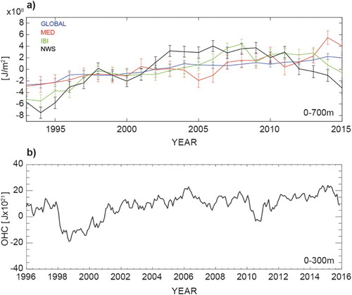
The positive Earth’s energy imbalance as currently measured (e.g. Trenberth et al. 2014) is related to an ongoing accumulation of energy in the Earth climate system manifested primarily as a warming of the global ocean (Figure 28). This overall warming is also dominating observed regional changes around Europe as seen during the last three decades (Figures 28 and 27(a) on average) at rates of 0.8 ± 0.2 in the Mediterranean Sea basin, 0.9 ± 0.3 in the Iberian-Biscay area and 0.8 ± 0.3 in the North-West Shelf. Strong signals of interannual variability are superimposed, and dominate the regional basin mean averages. For example, the Mediterranean Sea OHC time series is closely linked to the global time series, and is dominated by a distinct event during the years 2014–2015, when large temperature anomalies characterised the surface and intermediate waters of the Eastern Mediterranean, in particular the Southern Adriatic, the Ionian Sea and the Aegean (see Section 1.2).

Figure 28. Map of OHC decadal trends over the period 1993–2015 for the global ocean. Details on method and datasets used are described in the caption for Figure 28(a). Units are W/m².

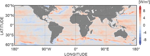
The decadal change in OHC varies with regions, as it is affected by ocean circulation and other physical features (e.g. Forget & Wunsch 2007), and by large-scale air–sea interactions (e.g. Trenberth & Fasullo 2010; Josey et al. 2013; L’Ecuyer et al. 2015). For example, and as discussed above, the Tropical Pacific Ocean shows particularly strong positive and negative anomaly changes due to the impact of El Niño-Southern Oscillation (ENSO) and the PDO. Regional patterns of decadal cooling occur in some areas of the world ocean, such as for example the North Atlantic (see Section 4.2). Nevertheless, an overall warming signal is dominant, in particular in the Atlantic and Indian Oceans, as well as in the Southern Ocean areas (Figure 28). The latter is known to be the strongest contributor to global mean OHC positive trends (Roemmich et al. 2015, Trenberth et al. 2016). The Mediterranean Sea presents a warming trend in its eastern basin, with maximum values in the Ionian and Southern Adriatic Sea, where the general circulation was completely modified by the NIR (Pinardi et al. 2015) in 1997 and a southward shift of the Atlantic Ionian Stream (see also Section 3.1).

2.2. Ocean mass and heat transport

Leading authors: Clement Bricaud, Yann Drillet, Gilles Garric

The state of the large-scale oceanic circulation, driven by wind, density gradients and tides, has a large impact on the climate of the Earth. Wind-driven surface currents systems (such as the Gulf Stream) travelling poleward transport heat from the equator, cooling en route, and, when eventually sinking at high latitudes, form deep waters with unique Temperature/Salinity (T/S) characteristics (see Section 2.3). These dense waters flow into the ocean basins and transport cold water from the poles back to the tropics. Thus, currents, with their transports of energy and mass, regulate global climate, helping to counteract the uneven distribution of solar radiation reaching the Earth’s surface.

Various estimates of global heat and mass transports at key areas of the ocean have already been proposed from direct ocean hydrographic sections (Talley et al. 2003), from the World Ocean Circulation Experiment (WOCE)-based inverse model using hydrographic data (Ganachaud 2003; Lumpkin and Speer (2007), and from ocean reanalysis (Stammer et al. 2004; Valdivieso et al. 2014). Observing systems have been developed and maintained to monitor the AMOC (RAPID array, McCarthy, Smeed, et al. 2015, see also Section 2.3), heat and volume transports are regularly estimated in choke points such as the Indonesian Throughflow (INSTANT program, Vranes & Gordon 2005; Gordon et al. 2008), the Drake Passage (Cunningham et al. 2003; Provost et al. 2011) and in the Southern Atlantic Ocean (Swart et al. 2008).

Here the CMEMS global ocean reanalysis product GLORYS is used (see Section 1.6 and endnote 13). Time–mean (1993–2015) transports for volume (top) and heat (bottom) are in the range of values obtained by Lumpkin and Speer (2007) estimations (Figure 29). Linear trends estimated at these sections are weak and not statistically significant (as such are not shown). The eastward Antarctic Circumpolar Current volume transport is estimated at 130 and 140 SV with associated heat transport ranging between 1 and 2 PW. In the Atlantic Ocean and Northern Pacific, estimated errors of volume transport from Lumpkin and Speer (2007) are an order of magnitude larger than the mean value. A northward heat transport is, however, depicted in the Atlantic Ocean in both estimates with good agreement. The volume transport between the Pacific and Indian Oceans is estimated from 13.3 SV in Lumpkin and Speer (2007) estimations to 17.7 SV in GLORYS. This large discrepancy is likely due to the multiple pathways within the Indonesian seas, differences in interannual variability and missing processes such as tides in GLORYS.

Figure 29. Mean 1993–2015 (a) volume (Sverdrup (SV = 10⁶ m³/s)) and (b) heat (Petawatt (PW = 10¹⁵ Watt) transports across the WOCE sections (green) from GLORYS reanalysis (see Section 1.6, endnote 13) (in red) with interannual standard deviation and Lumpkin and Speer’s (2007) estimations (in blue) with associated error. Arrows indicate the direction of the transport (positive in the northward and eastward directions).

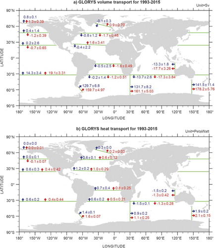
The global time–mean meridional heat transport (MHT, Figure 30) is in good agreement with previous estimates found in ocean reanalysis or derived hydrographic estimates. Coincident with strong narrow western boundary and poleward currents (Brazil and Somali currents), the oceanic MHT is characterised at the equator by a strong gradient. The MHT peaks (2.76 PW) at 3.50°N with highest interannual variability (up to 0.5 PW) in the tropical band due to string western boundary currents such as the Gulf Stream, the Kuroshio and the Somali and East Australian currents and due to the southward current pathways of the Indonesian Throughflow. Lower values in terms of amplitude and variability are found at high latitudes. In the 15°S–15°N band, values during the year 2015, lower than the GLORYS climatology, show a weakening of heat transport in the Northern Hemisphere and a strengthening in the Southern Hemipshere; Poleward MHT is however weaker between 30°S and 15°S and higher in the 15°–30°N bands. No noticeable changes were found in 2015 at high latitudes.

Figure 30. Time–mean (1993–2014) meridional heat transport (PW) for the global ocean (zonally and from surface to bottom integrated over the global ocean) estimated from GLORY reanalysis (see Section 1.6, endnote 13). The year 2015 is superimposed in red.

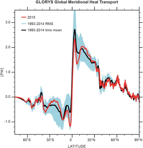
2.3. The Atlantic meridional overturning circulation

Leading authors: Clotilde Dubois, Vidar S. Lien.

Contributing authors: Marie Drevillon, Roshin P. Raj.

The AMOC plays a key role in the North Atlantic climate. The AMOC controls global ocean climate at decadal and longer time scales, as well as the formation of new water masses. The new water masses sink from the surface to the deep ocean and ventilate and renew water layers of the interior ocean. Recent observations of the AMOC at 26°N from the RAPID array suggest that a weakening has occurred in the past decade associated with a decrease in the density of Labrador Sea Water, which lags a decrease in the AMOC by a few years (Smeed et al. 2014; Jackson et al. 2016). Such changes in the North Atlantic are driven by physical interactions at the atmosphere–ocean interface controlling heat and momentum transfer but also by freshwater inflow from the Arctic, which in turn induces changes in the North Atlantic density field (Rahmstorf et al. 2015). At depth, the heat content in the North Atlantic has also shown a decrease since 2007 after a warming phase since 1980 (Häkkinen et al. 2015). The interplay of these different physical processes in this area is modulating climate variability, in particular over the European continent and North America. A particularly strong cold signature has been observed in the North Atlantic region in recent years (Section 4.2), which may affect the climate in Europe (Jackson et al. 2015; Duchez et al. 2016).

Using the CMEMS global ocean reanalysis GLORYS (see Section 1.6, endnote 13) the AMOC was evaluated and compared with the observations from the RAPID array (Figure 31). The modelled AMOC is in good agreement with observation data in terms of temporal variability, although the model tends to be underestimated with an average of 14.4 Sv compared with the observation mean of 17 Sv (Smeed et al. 2016). However, further analysis is needed in a multi-ensemble approach to further quantify the uncertainty range which can be large as shown in Karspeck et al. (2015). Such an analysis framework covering the AMOC along the RAPID section is planned for future activities on ocean monitoring within CMEMS. The 10-day average time series between the ocean reanalysis and the observations are correlated at 0.86 and a trend of −0.41 ± 0.18 Sv/yr measured at the RAPID array during the observation period is found. However, no significant trend was found over the period of the reanalysis (1993–2015).

Figure 31. Time series of maximum AMOC at 26°N in Sv from the reanalysis GLORYS (see Section 1.6, endnote 13) in blue and from the RAPID array in red, plotted with a running mean of 10 days (thin line) and with a 3-month running mean (thick solid line).

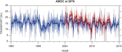
The North Atlantic is subject to a strong air–sea heat exchange which is dominated by exceptionally strong latent and sensible heat loss, associated with anomalously strong north-westerly winds, bringing exceptionally cold and dry air across the northeast Atlantic such as in the winter of 2010. These northerly air flows appear to be connected to climate modes such as the East Atlantic Pattern (EAP) and the NAO (Josey et al. 2015). The variability of the AMOC can be related to:

• During the period 1990–2004, the strengthening of the ocean circulation was due to persistent positive NAO (Robson et al. 2012; Yeager et al. 2012).

• During the period 2005–2014, negative trends were observed with a cooling of the North Atlantic. Changes in atmospheric circulation were observed but do not explain everything as the winter of 2013/2014 saw a very strong heat loss (Grist et al. 2016).

The AMOC is also controlled by the southward/return flow from high latitudes, i.e., Arctic and sub-Arctic (Figure 32). While the Labrador (e.g. Våge et al. 2009; van Aken et al. 2011) and Irminger (e.g. Våge et al. 2011; de Jong et al. 2012; Gladyshev et al. 2016) seas both contribute to the AMOC through deep water convection and subsequent dense water formation, the focus here remains on the Nordic Seas part of the dense water flow from north to south. The return/southward flow of the AMOC consists of several branches; one through the Faroe-Shetland Channel (FSC) (e.g. Borenäs & Lundberg 2004), one over the Iceland Faroe Ridge (Hansen & Østerhus 2000) and one through the Denmark Strait (DS) (e.g. Jochumsen et al. 2012), the latter being the largest with about 50% of the overflow (Jochumsen et al. 2012). The dense water (σ_θ > 27.8) overflow through these openings represents the integrated contribution from the dense water formation within the Arctic to the Arctic–North Atlantic exchanges (Figure 32). Such dense water formation mainly occurs in hotspots including the banks within the Barents Sea (Midttun 1985), Storfjorden in the Svalbard archipelago (e.g. Skogseth et al. 2008) and the area surrounding the Franz Josef Land and Severnaya Zemlya archipelagos (e.g. Martin & Cavalieri 1989), although some formation also takes place in the open ocean including the Greenland and Norwegian seas (e.g. Clarke et al. 1990). However, common to all the formation sites is the availability of Atlantic-derived water masses, which yields high enough salinities (typically S > 34.9) for the water masses to become dense enough to sink into the deep ocean through cooling and/or brine rejection associated with ice freezing.

Figure 32. Maximum mixed layer depth in the North Atlantic from the reanalysis GLORYS (see Section 1.6; endnote 13) over the period 1993–2015. Red arrows indicate major pathways for Atlantic Water flow into the Nordic Seas. Blue arrows indicate pathways for dense water overflow from the Nordic Seas to the North Atlantic. Red lines show key oceanographic sections: A – Faroe North section; B – FSC; C – Svinøy Northwest section; D – Barents Sea Opening; E – Fram Strait; F – DS.

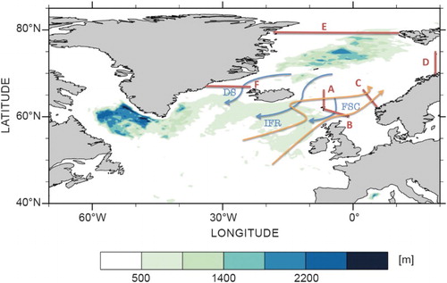
The CMEMS regional reanalysis product for the Arctic area (see Section 1.7, endnote 14) has been further examined for the 1993–2014 period, and the time series extended until 2015 using the CMEMS regional forecast product for the Arctic area (see Section 1.7, endnote 15). Model-based estimates of the DS overflow yielded an average overflow transport of 1.1 Sv through the DS during the period 1996–2011, which is only about one-third of the volume transport estimated based on direct current observations for a similar period (Figure 33). Furthermore, according to the model results, the dense water (σ_θ > 27.8) outflow through the FSC has decreased somewhat in recent years, and the 2015 overflow was only half of the 1993–2015 modelled average of 0.5 Sv, continuing a trend of lower overflow in recent years. The dense water overflow through the DS displayed a larger than average seasonal variation in 2015, with lower than average overflow in spring and autumn. On average, the overflow was less (0.7 Sv) compared with the 1993–2015 modelled average (1.0 Sv).

Figure 33. Volume transport time series of overflow waters as estimated from the CMEMS regional reanalysis and forecast product for the Arctic area (see text for more details). (a) Net volume transport of water masses with σ_θ > 27.8 through the Færøy-Shetland Channel. Negative indicate transports towards the south. Black line shows monthly averages and grey-shaded area denotes associated standard deviation. (b) Similar to (a), but showing for the DS. The reanalysis has been evaluated against observations in terms of ocean transports (Lien et al. 2016). The operational product is evaluated internally against observations on a weekly basis.

However, different results of sensitivity of the AMOC to freshwater flux are still controversial. Some of these studies suggest that AMOC strength is sensitive to Greenland melting (Fichefet et al. 2003; Brunnabend et al. 2015; Yang et al. 2016) while others do not (Ridley et al. 2005; Jungclaus et al. 2006; Hu et al. 2011). The recent paper by Rahmstorf (2015) found a decrease in the AMOC since the 1970s. Rahmstorf et al. (2015) links it with a freshwater anomaly known as the great salinity anomaly due to export from the Arctic. In addition, an increase in river discharges into the Arctic Ocean plus melt water from the Greenland ice sheet is observed.

The meridional overturning shows multi-decadal variability; however the North Atlantic water experienced an unprecedented cold event in 2015 (Section 4.2). The interplay between the Atlantic cold event and the Atlantic variability is still under investigation. Many studies are now predicting a cooling of the North Atlantic (Hermanson et al. 2014; Klöwer et al. 2014; Robson et al. 2014; McCarthy, Haigh, et al. 2015) and the key questions are if, and when, the North Atlantic will enter a cold phase as global climate models predict a weakening of the AMOC in future climate change, or is it still part of the decadal variability?

2.4. Mesoscale activity

Leading authors: M.-I. Pujol, Q. Dagneaux, A. Melet, A. Samuelsen, R. P. Raj, S. Simoncelli, M. Juza, J. Tintore, R. Morrow and K. von Schuckmann.

Mesoscale and sub-mesoscale eddies and meanders are ubiquitous in the ocean. Their energy generally exceeds the energy of the mean flow by an order of magnitude or more. Baroclinic and barotropic instabilities of the mean flow (Stammer & Wunsch 1999), Ekman pumping induced by wind fluctuations (Gill et al. 1974) and baroclinic instability generated by bottom roughness in shallow topography (Gille et al. 2000) are the main processes responsible for mesoscale eddy generation. Sub-mesoscale structures induced by mixed-layer instabilities (Stone 1966) can also feed energy up to mesoscale eddies through an inverse kinetic energy cascade (Klein et al. 2008). Mesoscale structures are also impacted by seafloor roughness, with higher energy dissipation in the deep ocean where there is important bottom roughness through friction (Arbic & Flierl 2004) and internal lee-wave generation (e.g. Nikurashin & Ferrari 2010; Melet et al. 2015).

Mesoscale and sub-mesoscale eddies interact with the mean flow (Holland 1978; Qiu & Chen 2010) and largely contribute to vertical exchanges in the upper ocean (Klein & Lapeyre 2009). They influence the large-scale circulation at the surface and in the deep ocean (Morrow et al. 1994) and thus contribute to the ocean’s role in the Earth’s climate system. Eddies also play a key role in the transport and budget of different tracers (heat, salt, nutrients, etc.) (Lee et al. 1997; Dufour et al. 2015) and have a large impact on physical-biological coupling at all trophic levels from phytoplankton (Gaube et al. 2014) and zooplankton (Gorsky et al. 2002) to the spatial distribution of fish in longer-lasting structures (Godø et al. 2012). The monitoring of the mesoscale and sub-mesoscale variability is thus an essential issue in the monitoring of the ocean, climate and ecosystem states.

In this report, the mesoscale activity based on the Eddy Kinetic Energy (EKE) monitored from satellite altimetry observations described by Pujol et al. (2016) and based on the global CMEMS reprocessed product (see Section 1.4, table footnote c) is assessed. Previous studies show the capability of the altimeter measurements to capture the mesoscale variability over the global ocean since 1993, i.e. from the precise altimetry era and when at least two different altimeters were available to sample the ocean surface (Ducet et al. 2000). The capability of altimetry to sample the mesoscale signal has largely been improved since mid-2002, when three to four altimeters were available (Pascual et al. 2006). Note however that only the larger part of the mesoscales can be monitored with the gridded altimetry product since it currently only captures the larger wavelengths > 200 km, corresponding to feature scales greater than 100 km (Chelton et al. 2011).

2.4.1. General overview of the mean Eddy Kinetic Energy:

The EKE level is generally commensurate with the intensity of the current, with greater energy in the vicinity of the main jets and currents characterising the ocean surface circulation and associated permanent/recurrent structures (Figure 34). The highest levels of EKE (more than 2000 cm²/s²) are observed in the western boundary currents such as the Gulf Stream and the Kuroshio, and along the Antarctic Circumpolar Current. Equatorial waves also contribute to high EKE in the equatorial band. Elsewhere, the EKE amplitude rapidly falls off by at least an order of magnitude. The comparison of the mean EKE observed in 2015 with the 1993–2015 climatological mean (Figure 35) shows significant differences (up to ± 200 cm²/s², representing from 50 to more than 100% of the mean EKE climatology mean) characterising the interannual variability of the mesoscale structures. This report focuses on the description of EKE variations in the Gulf Stream and Mediterranean Sea.

Figure 34. Climatological mean EKE computed from daily data (see Section 1.4, table footnote c) over the 1993–2015 period for the (a) global and (b) Mediterranean Sea (note the different colourbar range).

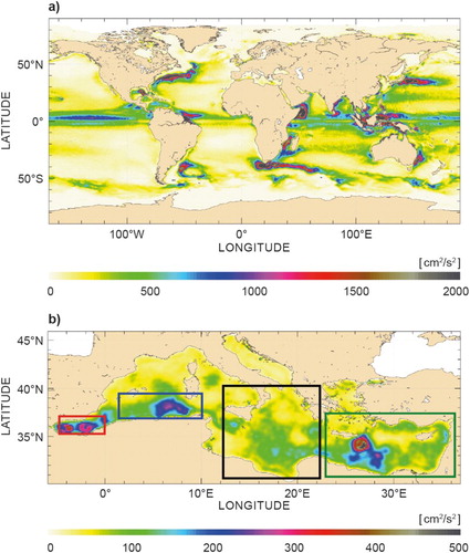
Figure 35. Anomalies of EKE for 2015 [09/2014–08/2015] with respect to the [1993–2014] climatological mean over the global ocean (a) and Mediterranean Sea (b) (note the different colourbar range).

2.4.2. Gulf Stream

The Gulf Stream mean and eddying flows largely contribute to the distribution of energy and biogeochemical properties in the North Atlantic Ocean. The EKE monitored in the Gulf Stream region shows a clear seasonal variability, with maximum levels in the summer period (May to September) and minimum levels in winter (January). Recent regional modelling analyses also indicate the presence of two dominant peaks in EKE related to the short-lived (< 1 month) structures in the offshore Gulf Stream region in May, with a secondary peak in September near the surface (Kang et al. 2016). The mechanisms explaining this seasonality are associated with seasonal buoyancy forcing that impacts the flow’s baroclinic instability and is related to the May peak of the upper ocean EKE, whereas the September peak is mainly affected by advection of energy from remote regions, giving rise to correlations with the seasonal cycle of remote winds. Additional contributions of the seasonal modulation of eddy damping by the wind stress (Duhaut & Straub 2006) and of the inverse cascade of energy from the sub-mesoscales to the mesoscales (Sasaki et al. 2014) have been pointed out.

The EKE variations over the Gulf Stream also exhibit major interannual variability. A decrease in the Gulf Stream EKE was observed in 2005 that mainly occurred in the eastern part of the Gulf Stream (east of 60°W) and was coupled with an attenuation of the seasonal variations afterward. In 2015, EKE levels in this part of the Gulf Stream also remained lower than average. The weakening of the EKE observed after 2005 might be linked to the decline of the AMOC observed from 2004 onwards (Robson et al. 2014), but further investigations are needed to better understand the causes of this weakening. In the western part of the Gulf Stream (west of 60°W), the EKE levels were slightly higher than average in 2015, revealing a more turbulent than average Gulf Stream (Figure 35).

2.4.3. Mediterranean Sea

The mesoscale activity in the Mediterranean Sea is characterised by a large number of permanent or recurrent structures that interact with and modify the mean flow (see also Section 3.1). In the Alboran Sea (red box in Figure 35), the observation of mesoscale dynamics with altimetry is quite challenging due to the narrow geometry of the basin and the ubiquitous presence of the coasts. Nevertheless, Juza et al. (2016) showed that the recent improvement in altimeter data processing allows an accurate observation of the Western and Eastern Alboran Gyres that define the mean circulation in the basin (see Section 3.1). The energy of these structures is strongly modulated by the fluctuation of the Atlantic water inflow (Tintoré et al. 1991, among others). In 2015, the EKE of these structures exceeded the climatological mean value by nearly 200 cm²/s² (Figure 35), underscoring their annual and interannual variability. During this year, the Western Alboran Gyre was well defined, especially during the summer period when it reaches its maximal intensity (Heburn & La Violette 1990; Vargas-Yanez et al. 2002). However in 2015, the Eastern Alboran Gyre was absent.

Along the Algerian coast (blue box in Figure 34), the mesoscale activity is mainly characterised by intense anticyclonic eddies (Algerian eddies) that are generated by Algerian Current instabilities. Algerian eddies are usually advected eastward by the Algerian Current up to the Sicily Channel, where they can detach and turn to propagate westward into the central western basin (Millot 1985). Previous studies have shown that the energy of the Algerian eddies is subject to high annual (maximum energy in winter) and interannual variability (e.g. Molcard et al. 2002; Pujol & Larnicol 2005). In 2015, the mesoscale activity was weaker than its climatological mean value along the Algerian Current, west of 5°E, suggesting that few Algerian eddies were created during this year in this area. Actually, only one intense Algerian eddy was created near 1°E in July. In contrast, the positive EKE anomalies observed southwest of Sardinia (nearly + 150 cm²/s²; Figure 35) are linked to the high variability in this area, induced by propagating Algerian eddies and possibly also Sardinian eddies (Testor & Gascard 2005).

In the Ionian Sea (black box in Figure 34), the mesoscale activity is strongly correlated with the surface flow path in the basin (Pujol & Larnicol 2005). Satellite and in situ observations, as well as model simulations, all indicate the circulation changes in the basin in the past, the last ones occurring in 1986–1987 and 1997 (Malanotte-Rizzoli et al. 1999; Klein et al. 1999; Larnicol et al. 2002; Rupolo et al. 2003; Pinardi et al. 2015). In 2015, the Atlantic Ionian Stream (Robinson et al. 1999) is observed in the southern part of the basin (see Section 3.1). Its instabilities create meanders and eddies in its vicinity explaining the positive EKE anomalies (∼ + 100 cm²/s²) observed in this area (Figure 35). In the Levantine basin (green box in Figure 34), EKE positive anomalies ranging between + 150 and 300 cm²/s² (Figure 35) underscored the Mersa-Matruh (Robinson et al. 1991) and Shikmona Gyre Systems that were quite visible in 2015 (Section 3.1). The Ierapetra Eddy, usually located in the Crete’s south-east corner, is not visible during the year 2015.

Chapter 3: Regional Seas

The CMEMS also provides regular and systematic core reference information on the state of the regional seas. CMEMS regions include the Mediterranean Sea basin, the North-West Shelf (NWS), the Arctic Ocean, the Baltic Sea, the IBI Sea and the Black Sea. The Black Sea is not discussed in this chapter as the CMEMS and product delivery to users in this area started in October 2016. The regional specifications are given in Figure 1. A large-scale view of the surface circulation and hydrographic changes has been developed for the Mediterranean Sea (Section 3.1) and NWS areas (Section 3.2) with a particular focus on the anomalous changes that occurred during 2015. Changes at specific regional key choke points are reported in the other sections. Those are known to have major impacts not only on the physical ocean state, such as changes in sea level and energy redistribution, but also on the regional ecosystems, carbon cycles and fisheries. They are associated with noticeable societal impacts. These choke points include water mass exchange pathways and related changes during the period 1993–2015 from the North Atlantic into the Arctic Ocean (Section 3.3) and from the North Sea into the Baltic Sea (Section 3.4), as well as coastal upwelling processes along western Iberian and African continental shelves (Section 3.5). This chapter is a first, but important, step forward in order to respond to the need of improving knowledge of the environmental status of the regional marine waters as required, in particular, for the MSFD currently implemented by European Member States. The development of the CMEMS OSR and its associated marine environment monitoring activities is expected to provide, in the upcoming years, support to decision-makers implied in policies linked to the marine environment (e.g. EC Directorates, EEA, ICES, and Regional Seas Conventions).

3.1. Mediterranean Sea

Leading authors: Simona Simoncelli, Gerasimos Korres, Nadia Pinardi

Contributing authors: Claudia Fratianni, Emanuela Clementi, Joaquin Tintoré

The Mediterranean Sea is of economic, environmental and cultural importance and is adjacent to a number of European countries as well as countries in eastern Asia and northern Africa. The general circulation of the Mediterranean Sea, its past evolution, present variability, trends and future changes have been the subject of many studies. Due to its relatively small size and semi-enclosed nature, the Mediterranean climate is very sensitive to atmospheric forcing and anthropogenic influences.

The circulation is driven by three major external forcing agents: the wind, the inflow/outflow at the Gibraltar Strait and the buoyancy fluxes at the air–sea interface. Rivers and the Dardanelles inflow/outflow further modify the basin freshwater budget and the dynamics at a local scale. Water loss by evaporation exceeds, on an annual basis, the fresh water input from precipitation and river input. The resulting fresh water deficit is compensated by a net inflow from the Atlantic. In return, the Mediterranean exports to the Atlantic Ocean saline waters that are produced at intermediate depths in the eastern part of the basin.

The Mediterranean Sea is characterised by three thermohaline cells partially driven by dense water (intermediate and deep) formation processes: a basin-wide longitudinal open cell, with a freshwater inflow from the Atlantic and a Levantine deep water outflow at the Gibraltar Strait, and two separated meridional cells in the western and the eastern parts of the basin. The Eastern Mediterranean thermohaline cell changed in the 1990s, when dense-water formation in the Adriatic was replaced by the Cretan Sea dense waters (Eastern Mediterranean Transient). This climate phenomenon might be related to the NIR (Pinardi et al. 2015), the Atlantic Water pathway, the Dardanelles inflow and severe wintertime heat losses.

The present section aims to review the general surface circulation of the Mediterranean Sea using 27 years (1987–2014) of CMEMS regional reanalysis (see Section 1.2, endnote 8; Meccia et al. 2016; Simoncelli et al. 2016), considering as a reference the work of Pinardi et al. (2015), whose synthesis is instead based on the 23-year reanalysis (1987–2007) carried out by Adani et al. (2011). Please refer to Figure 12 of Pinardi et al. (2015) for a schematic of the mean surface circulation structures and Table 2 of Pinardi et al. (2015) for the adopted nomenclature. The 2015 mean surface circulation computed from the CMEMS regional analyses (see Section 1.2, endnote 9) is then described pointing out the main differences with the climatological one. Both reanalysis and analysis fidelity have been validated extensively using adopted standard procedures (Maksymczuk et al. 2016; Simoncelli et al. 2016). The second part of the section will focus on the decadal variability of the circulation in the Ionian basin, its impact on the salinity distribution and link to the main water mass formation events in the Eastern Mediterranean.

The general surface circulation computed over the 1987–2014 time period (Figure 36(a)) from reanalysis data shows the presence of open-ocean free jets – intensified structures like the Western Mid Mediterranean Current, the Atlantic Ionian Stream and the Mid Mediterranean Jet, as described in Pinardi et al. (2015). The Atlantic Water Current enters at Gibraltar and meanders around one or two anti-cyclonic gyres, the quasi-permanent Western Alboran Gyre (Juza et al. 2016) and the intermittent Eastern Alboran Gyre. The eastern boundary of the Eastern Alboran Gyre forms south of Cape Gata the Almeria-Orán front, an intense density front resulting from the convergence of Atlantic and Mediterranean waters that modifies the eastward propagation of the Atlantic Water Current. East of Orán, the Atlantic Water Current becomes the Algerian Current, a well-defined boundary current, which loses intensity between 4 and 8°E due to instability processes and the formation of large anti-cyclonic eddies that modify the basin-scale circulation with significant biogeochemical effects (Cotroneo et al. 2016). A branch of the Atlantic Water Current flows northeastward along the Ibiza Channel (Heslop et al. 2012), turns around the island of Majorca where it merges with the Liguro-Provencal-Catalan Current and becomes the Western Mid Mediterranean Current flowing eastward into the open ocean. It turns southward along the western coast of Sardinia, becoming the southerly Sardinia Current, one of the largest amplitude currents in the Western Mediterranean. Then it turns eastward along the Tunisian coast merging with the Algerian Current at around 8°E. The Algerian Current when exiting the Sardinia Channel branches into three parts, the northern branch entering the Southern Tyrrhenian Sea and the other two entering the Sicily Strait. The South-Western Tyrrhenian Gyre and the Northern Tyrrhenian Gyre dominate the Tyrrhenian mean circulation, while small-scale features characterise the south-eastern region weakening its mean cyclonic circulation. The Western and Eastern Corsica currents flow northward around the island, the former being part of the Gulf of Lion Gyre.

Figure 36. Mediterranean Sea circulation at 15 m: (a) computed from the CMEMS regional reanalysis product for the Mediterranean Sea over the time period 1987–2014; (b) computed from the CMEMS regional analysis data for 2015, see text for more details on data use.

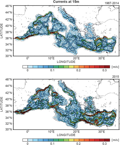
The Algerian Current enters the Sicily Strait as a two-jet structure, the Sicily Strait Tunisian Current flowing along the Tunisian coast and the Atlantic Ionian Stream meandering southeastwards along the Sicilian coast. East of Malta the Atlantic Ionian Stream crosses the Ionian Sea as a broad open ocean free jet meandering around 36°N with bifurcations into southerly branches. The Sicily Strait Tunisian Current turns northeastwards in the Gulf of Syrte to form two anti-cyclonic gyres that constitute the Syrte Gyre system. In the centre of the Ionian Sea the Atlantic Ionian Stream turns southward towards the African coast where it becomes an intense coastal current named the Cretan Passage Southern Current. In the eastern part of the Ionian Sea the anti-cyclonic Pelops Gyre is present, together with a series of cyclonic gyres, the northernmost referred to as the Corfu Cyclone (Horton et al. 1997). The Cretan Passage Southern Current branches in the Mid Mediterranean Jet and the Southern Levantine Current. The Mid Mediterranean Jet is the free jet between the Mersa-Matruh Gyre System in the south and the Rhode Gyre in the north. The Mid Mediterranean Jet meanders eastward south of Cyprus around the Shikmona Gyre System area, it merges the Southern Levantine Current to form the Cilician Current and then becomes the Asian Minor Current. A well-defined cyclonic eddy occupies the Antalya gulf (Onken & Yüce 2000). Part of the Asian Minor Current enters the Kassos Strait into the Cretan Sea to form the Cretan Sea Westward Current. Southeast of Crete the IeraPetra Gyre (Robinson et al. 1991; Pujol and Larnicol 2005) is present and the circulation southwest of Crete is dominated by the Western Cretan Cyclonic Gyre.

Figure 36(b) shows the mean surface circulation in 2015. The first important difference with the climatology is the higher intensity of boundary currents and free jets. Furthermore, persistent eddies appear in different areas, particularly in the Algerian basin, the Ionian Sea and the south-eastern Mediterranean. Looking at the differences in more detail – the first difference is in the Alboran Sea where the cyclonic feature between 2°W and 2°E is more intense than in the climatology. In the Sicily Strait, the weakening of the Atlantic Ionian Stream and strengthening of the Sicily Strait Tunisian Current are the major differences compared to the climatological circulation and explains the freshening of the Levantine and Aegean basins as indicated by surface (Figure 8) and subsurface (Figure 9(d)) salinity anomalies as in Section 1.3. The Levantine circulation is characterised by an intense Cretan Passage Southern Current, Mid Mediterranean Jet and Asian Minor Current, of larger amplitude than the climatology. Furthermore, the Mersa-Matruh Gyre is split into two centres, with one of them showing higher amplitudes than the other (see also Section 2.4). The Ierapetra Gyre is absent, as confirmed by satellite observations as described in Section 2.4.

Pinardi et al. (2015) identified the NIR as exhibiting the largest decadal variability event since 1987. The surface mean circulation in the Ionian Sea (Figure 37) over the time periods (a) 1987–1996; (b) 1997–2006 and (c) 2007–2014 confirms that the mean circulation in the Northern Ionian reversed from anti-cyclonic (a) to cyclonic (b) but then remained cyclonic (c). However, between 1987 and 1996 (a) the Northern Ionian was characterised by the northward shift of the Atlantic Ionian Stream and the large-scale flow field was dominated by anti-cyclonic motion. From 1997 to 2006 (b) the Atlantic Ionian Stream crosses the centre of the basin and the Northern Ionian is cyclonic, with different sub-gyre centres including, among others, the Corfu cyclone. In the period from 2007 to 2014 (c) the cyclonic circulation in the Northern Ionian weakened and several eddy centres formed on its eastern and western sides, always with a cyclonic general circulation. The averaged salinity along section A in Figure 38 confirms that the Atlantic Water is carried south of 37°N in periods (b) and (c), mainly by the Sicily Strait Tunisian Current and the Atlantic Ionian Stream is shown to have shifted southward.

Figure 37. Surface circulation in the Ionian Sea computed from the CMEMS regional reanalysis product (see text for more details) over three time periods: (left) 1987–1996; (middle) 1997–2006; (right) 2007–2014.

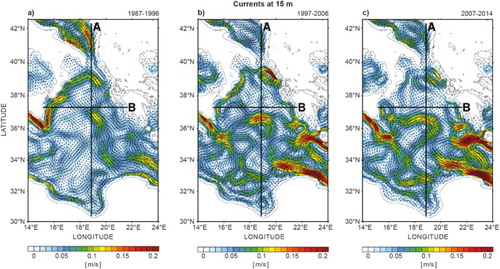
Figure 38. Mean meridional (left, 18.875°E) and zonal (right, 37.3125°N) salinity sections computed from the CMEMS regional reanalysis product (see text for more details) over three time periods down to 1000 m of depth: (top) 1987–1996; (middle) 1997–2006; (bottom) 2007–2014.

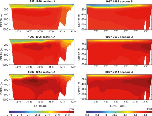
The main consequence of the described decadal variability of the Mediterranean circulation is a salinification of the Northern Ionian basin and the inflow of saltier waters into the Adriatic (Meccia et al. 2016) at intermediate depths as shown in section A in Figure 38 (see also Section 1.3). After 2007 (period c) the salinity increases in the layer 200–400 m with maximum values at 300 m between 34°N and 36°N. The averaged salinity along section B in Figure 38 shows the progressive spreading of Levantine and Cretan Intermediate Water westward with maximum salinity along the eastern Ionian flank.

The main water mass formation events in the Eastern Mediterranean were influenced by these important changes in the circulation patterns. In the first of the three decades, LIW and Levantine Deep Water formed in the Rhode Gyre area, the Eastern Mediterranean Deep Water weakened in the Southern Adriatic and a large amount of Cretan Deep and Intermediate Water formed in the Cretan Sea (Roether et al., 1996). During 1992–1993, the Cretan Deep Water reached maximum formation rates together with both LIW and Levantine Deep Water determining the Eastern Mediterranean Transient and causing a temperature and salinity increase of intermediate and deep waters (Pinardi et al. 2015). In 1999 the water mass properties of the Southern Adriatic changed abruptly due to the arrival at mid-depth of these saltier waters triggering a large Eastern Mediterranean Deep Water formation event (Manca et al. 2006) and the re-start of the Eastern Mediterranean Deep Water formation. A third Eastern Mediterranean Deep Water formation event happened during 2005–2006 in parallel with LIW formation in the Rhode Gyre. These events explain the spreading of salty waters in Figure 38 during the period 1987–1996 (a) to the period 1997–2006 (b) between 200 and 700 m depth and the occurrence of new saltier waters within 200–400 m along the eastern flank of the basin due to the Aegean outflow of Cretan Intermediate Water. New dense Cretan Intermediate Water produced in the Aegean Sea during 2007–2009 exited through the Cretan Straits and reached the Adriatic Sea (Velaoras et al. 2014), as confirmed by the averaged salinity sections in Figure 38 (period c). The further salinification of the Northern Ionian and Southern Adriatic Sea is likely to have contributed to the exceptional Eastern Mediterranean Deep Water formation event that occurred in 2012 (Mihanovic et al. 2013).

3.2. North-West European Shelf Seas

Leading author: Jonathan Tinker

Contributing authors: Enda O’Dea, Peter Sykes, Patrick Hyder, Jason Holt and Stephen Dye

The North-West European Shelf (NWS) seas are of economic, environmental and cultural importance and are adjacent to a number of European countries. The NWS has some of the strongest tides in the world with ∼200 GW tidal dissipation over the region (Egbert & Ray 2001). These tides are an important feature of the NWS and allow some regions to remain vertically mixed through the year, while other regions of the shelf seasonally (thermally) stratify (Otto et al. 1990). The Baltic Sea is an important source of relatively fresh water that is largely constrained to the Norwegian Coastal Current (NCC) as it leaves the NWS, and maintains year-round salinity stratification in the Norwegian Trench (NT). The permanent salinity stratification in the NT and its much greater depth means that the NT is quite different from the rest of the NWS.

The NWS seas have a complex circulation pattern driven by a combination of wind, density and large-scale (sea surface slope) forcing (Hill et al. 2008; Holt & Proctor 2008). The main features of this circulation pattern (see OSPAR 2000, Figure 2.3) are: the north-eastward shelf-break current to the west and north of Ireland and Scotland; the westward and then northward NCC following the Norwegian coast out of the Skagerrak; and the adjacent southward current flowing offshore, and in opposition to the NCC; the Dooley current, flowing eastwards across the North Sea roughly following the 100 m isobaths (at ∼58°N) and the generally anti-clockwise circulation of the North Sea. In the climatology, the mean summer and mean winter surface currents are fairly similar, in configuration, but with a greater magnitude in the winter field; however, these climatology fields hide a range of different patterns of circulation. The circulation in the Celtic Seas is weaker and more variable than the North Sea, but is generally northward and eastward into the Irish Sea and English Channel. In the summer, seasonal stratification produces fronts, which restrict cross-frontal transfer.

While many properties of the NWS are subject to a strong seasonal cycle (such as temperature), the synoptic and year to year variability is often important. A comparison is made looking at how the surface currents (and winds) of 2015 compare to the mean of the 1994–2013 period, and consider how typical 2015 is by showing where the current magnitudes of 2015 fits within the distribution of the 1994–2013 period.

For this first OSR, surface currents are focused on (upper grid box, typically the upper 1 m), which are heavily influenced by the surface wind field. In future reports, depth mean currents will be included (not available for this report). It is noted that 2015 is taken from the CMEMS regional near-real-time forecast analysis¹⁸ and that 1994–2013 is from the CMEMS regional reanalysis;¹⁹ as such these products can be compared during the 4-year overlap period in terms of shelf mean current magnitude bias (0.04 cm/s) and shelf mean temporal correlation (r = 0.76). The near-real-time product for 2015 is not bias corrected.

The climatological (1994–2013) surface currents (and winds) are compared to 2015 currents in Figure 39. Overall the 2015 surface current configuration was similar to the climatology, but with stronger magnitudes. The 2015 annual mean is very similar to the baseline in terms of its pattern, but with much greater magnitudes. In the 2015 winter there is a generally eastward/south eastward current in the North Sea, which appears as an additional current at ∼56° N. There is also an eastward current around Southern Ireland and across the Celtic Sea in winter 2015, which is absent in the baseline mean. In the summer, the shelf-break and coastal currents northwest of Ireland and Scotland are much stronger in 2015 compared to the baseline.

Figure 39. Mean surface currents and wind, annual, winter (DJF) and summer (JJA) mean (left to right) for the 1994–2013 climatology (upper row), 2015 (middle row) and anomaly (2015 minus the 1994–2013 climatology). Streamlines show the 10 m winds. The colours show the surface current magnitude (m/s) (log scale for the upper and middle rows) with the current directions given with vectors. These are shaded off the shelf. The anomaly (bottom row) shows 2015 minus climatology. For example, colours representing a positive value reflect a stronger current magnitude in 2015 than in the 1994–2013 mean, and the vectors show how the current direction has changed.

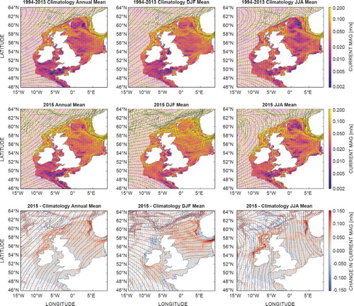
The individual annual (and winter/summer) means for each year within the baseline period (1994–2013) as a distribution are considered, and to where 2015 fits within this distribution. This is more powerful than simply looking at the mean of this distribution (i.e. the climatology) as it shows how typical, or unusual, 2015 is relative to the recent past. The 2014/2015 winter was particularly windy, with most of the northern shelf region being windier than any other time within the baseline period. In the summer, there are southwest/northeast bands of wind stronger and weaker than average wind. The annual mean wind strengths follow the winter, being stronger than most years from the baseline.

When comparing the surface current magnitudes to those from the baseline distribution there is much more spatial heterogeneity (Figure 40). The 2015 surface current magnitudes (particularly for the winter and annual means) tend to be stronger than most years within the baseline period, and this is consistent with being stronger than the baseline mean. It is interesting that most of the 2015 winter surface current magnitude strengths from the North Sea were generally greater than those from the baseline period. In the summer most of the 2015 North Sea current magnitudes are stronger than in the baseline although not along the British east coast, or in regions of the NCC and northern North Sea. The 2015 summer Celtic Sea and western English Channel current magnitudes tend to be weaker than most years in the baseline distribution. In the annual mean, most current magnitudes tend to be stronger than most years from the baseline, except in the Celtic Sea and western English Channel.

Figure 40. The climatology represents the mean of the years between 1994 and 2013; however these individual years can be expressed as a distribution. Here we ask where the 2015 wind and surface current magnitude fit within the distribution of values from 1994 to 2013, for the annual mean (ANN), winter (DJF, for 2014/2015) and summer (JJA) (left to right), for the magnitude of the 10 m wind and surface currents (upper row and lower row, respectively). The values off the shelf are greyed out. To highlight the extreme values, the values from the centre of the distribution (within 20th to 80th percentile) are lightly greyed out.

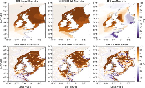
The NWS surface currents in 2015 were much stronger than in most years within the 1994–2013 baseline period. The 2014/2015 winter had anomalously strong current magnitudes over most of the North Sea and Celtic Sea, while the 2015 summer had anomalously strong currents west and north of Ireland and Scotland, but weaker currents in the Celtic Sea. These combined in the annual mean to give anomalously strong current magnitudes in the North Sea, western English Channel and west and north of Ireland and Scotland. In the annual mean, the current magnitudes in the Celtic Sea were much closer to, or below, the median of the baseline period.

3.3. North Atlantic – Arctic exchanges

Leading author: Vidar S. Lien

Contributing author: Roshin P. Raj

The northward flow of relatively warm and saline Atlantic Water through the eastern Nordic Seas and into the Arctic, balanced by an outflow of cold Arctic water masses through the western Nordic Seas, governs the exchanges between the North Atlantic and the Arctic as well as the distribution of oceanic heat within the Arctic (e.g. Mauritzen et al. 2011; Rudels 2012). However, the pathway of the Atlantic Water determines the fate of its heat content: the Atlantic Water entering the Arctic through the Fram Strait retains a large part of its heat as it flows cyclonically along the Arctic Ocean shelf slope (e.g. Polyakov et al. 2005), whereas the Atlantic Water that enters the Barents Sea loses most of its heat before it enters the Arctic Ocean through the St. Anna Trough (e.g. Lien & Trofimov 2013). In addition to the transport of heat, the Atlantic Water also transports nutrients and zooplankton (e.g. Sundby 2000), and it carries large amounts of ichthyoplankton of commercially important species, such as Arcto-Norwegian cod (Gadus morhua) and Norwegian spring-spawning herring (Clupea harengus) along the Norwegian coast. The Atlantic Water flow thus plays an integral part in defining both the physical and biological borders between the boreal and arctic realm. Variability of the Atlantic Water flow to the Barents Sea has been found to move the position of the ice edge (Onarheim et al. 2015) as well as the habitats of the various species in the Barents Sea ecosystem (Fossheim et al. 2015).

The Atlantic Water flow towards the Arctic has been monitored regularly by direct current measurements for a couple of decades in key sections (see Figure 32 for sections locations): the FSC (since 1994) (Berx et al. 2013); the Faroe North section (e.g. Østerhus et al. 2005); the Svinøy Northwest section (since 1995) (Orvik et al. 2001); The Barents Sea Opening (since 1997)(Ingvaldsen et al. 2002); and the Fram Strait (since 1997) (Schauer et al. 2004). In addition, these sections are monitored through hydrographic sections with the coverage frequencies varying from one to several per year.

The flow of Atlantic Water through the FSC amounts to 2.7 Sv (Berx et al. 2013). The corresponding model-based estimate is 2.0 Sv for the period 1993–2015. The model-derived Atlantic Water inflow, based on the CMEMS regional model (see Section 1.7, endnote 15), was at the lowest during 2014 and 2015 in the whole 1993–2015 time series (Figure 41), especially during the summer when the monthly anomalies were between 2 and 3 standard deviations below the 1993–2015 average. Moreover, the model indicates occasional reversals of the Atlantic Water flow. These volume transport anomalies are also reflected in similar, negative heat transport anomalies (not shown). Such strong anomalies indicate a fundamental, temporal change in the underlying forcing mechanisms, with the consequences expected to spread downstream into the Nordic Seas in the coming years.

Downstream in the Barents Sea Opening, the model indicates a long-term average Atlantic Water flow of 2.2 Sv, as compared with the long-term estimate from observations of 1.8 Sv (Smedsrud et al. 2013). During 2015, the inflow to the Barents Sea was above the seasonal average in March, which represents the time of the year with the highest inflow (Ingvaldsen et al. 2004), and closer to the long-term average in spring, which represents the most important period for the advection of zooplankon and ichthyoplankton. Later, during summer, the inflow was lower than average preceding a slight upwards turn in late autumn and winter. On average, the 2015 Atlantic Water inflow was close to the long-term average both in terms of volume and heat. In the Fram Strait, the model results indicate similar conditions to recent years, but less northward flow of Atlantic Water compared with the years 2005–2010, as the model indicates a shift in the flow regime of Atlantic Water in 2005, with a distinct increase as compared with previous years. This increase in Atlantic Water advection is likely, at least in part, attributable to increased temperatures during that period (e.g. Walczowski et al. 2012), and hence a larger fraction of Atlantic Water (T > 2°C). Changes in the heat transport to the Arctic have a multitude of impacts on the Eurasian Arctic, ranging from hydrography (e.g. Polyakov et al. 2012) to sea ice conditions (e.g. Ivanov et al. 2016) and distribution of species (e.g. Fossheim et al. 2015), as well as the net carbon uptake at high latitudes (e.g. Smedsrud et al. 2013).

3.4. Baltic Sea

Leading authors: Urmas Raudsepp, Lars Axell

Contributing authors: Elin Almroth-Rosell, Lena Viktorsson

The Baltic Sea is a huge brackish water basin in Northern Europe where precipitation exceeds evaporation. This implies that fresher water lies on top of water with higher salinity. As the Baltic Sea is connected to the North Sea only through very narrow and shallow channels in the Danish Straits, inflows of high-saline water into the Baltic occur only intermittently. Major Baltic Inflows (MBIs) bring large volumes of saline and oxygen-rich water into the bottom layers of the deep basins of the central Baltic. These MBIs occur seldom, sometimes many years apart (e.g. Matthäus & Franck 1992; Schimanke et al. 2014). The MBIs are forced by a characteristic meteorological sequence (Lass & Matthäus 1996; Schinke & Matthäus 1998). During the first phase, sustained easterly winds force an outflow from the Baltic and the sinking/falling of mean sea level. The second phase, i.e. inflow to the Baltic, starts with westerly winds and lasts until wind speed decreases and changes direction. Absence of MBIs causes weakening of the salinity stratification and worsening of oxygen conditions in the deep basins of the Baltic Sea. The MBIs turn anoxic conditions to oxic conditions in the bottom layers of the deep Baltic basins, which has a crucial effect on nutrient conditions (Nausch et al. 2003) and impacts the whole ecosystem from phytoplankton production up to the reproduction of Baltic cod (Plikshs et al. 2015).

During 2015, the most important change in the Baltic circulation was associated with the MBI, which had already started in December 2014. The 2014/2015 MBI was the third largest MBI recorded since 1880 and was double the strength of the previous 2003 event (Mohrholz et al. 2015). The development and dynamics of the 2014/2015 MBI in the south-western Baltic Sea are fully described by Mohrholz et al. (2015) and Gräwe et al. (2015). The estimated volume and salt transport were 281 × 10⁹m³ and 3.84 Gt (Gräwe et al. 2015), and 312 × 10⁹ m³ and 3.98 Gt (Mohrholz et al. 2015). In comparison, the total volume and salt content of the water layer below 150 m depth, i.e. the anoxic layers, were estimated at 285 km³ and 2.8 Gt, respectively.

The regional CMEMS forecast product²⁰ adequately reproduced the MBI in December 2014 compared to the measurements at the Marine Environment Observation Network (MARNET) station in the Arkona Basin (Figure 42). The first signal of increasing salinity on 12 December was not caught by the model as the depth of the model grid point is less than the actual depth in the area. The increase in salinity started on 16 December, which is consistent with the measurements. In general, the salinity in the model remained slightly lower than observed. The snapshots of bottom salinity (Figure 43(a)) and salinity transect from Oresund to the Bornholm Basin (Figure 43(b)) on 26 December show that inflow water has filled the Bornholm Basin. The period from 26 December onwards is considered as the post-inflow period (Mohrholz et al. 2015).

Figure 41. Volume transport time series of the Atlantic Water flow towards the Arctic. (a) Net volume transport through the Fram Strait (T > 2 °C). Positive values towards the north. Black line shows monthly averages and grey-shaded area denotes associated standard deviation. (b) Similar to (a), but showing for the Barents Sea Opening (N70° 15′ – N74° 15′; T > 3°C). Positive values towards the east (into the Barents Sea). Red line shows observations (N71° 30′ – N73 30′; T > 3°C). c) Similar to (a), but showing for the FSC (T > 5 °C). Positive values towards the north. For section positions, please see Figure 32. The model data are based on the CMEMS regional re-analysis product (see Section 1.7, endnote 14) for the years prior to 2015 and the CMEMS forecast product for 2015 (see Section 1.7, endnote 15). The reanalysis has been evaluated against observations in terms of ocean transports (Lien et al. 2016). The operational product is evaluated internally against observations on a weekly basis.

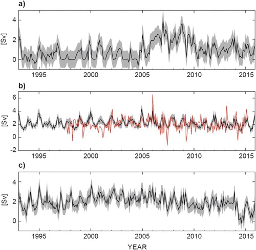
Figure 42. Salinity at the MARNET station in the Arkona Basin from observations (a) and reproduced by the CMEMS forecast product (see text for details) (b).

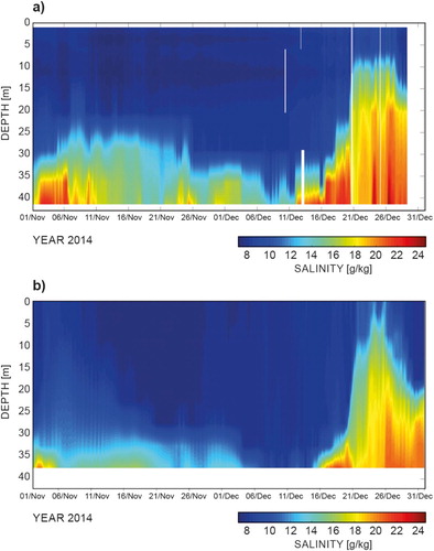
Figure 43. Bottom salinity (a) and salinity along the transect from Kattegat to the Bornholm Basin (b) from the CMEMS forecast product (see text for details) on 26 December 2014.

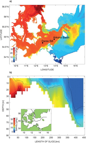
The MBI in December 2014 was followed by the next inflow in January 2015 as shown by the Hiromb Boos Model (HBM). The water salinity that reached the Arkona Basin exceeded 22 g/kg as shown by measurements (Figure 44(a)). Note that the MBI in December 2014 was not identified in the measurements. The salinity of 21 g/kg was measured on 10 November 2014 and corresponds to the increase in salinity at the beginning of November 2014 also seen at the MARNET station in the Arkona Basin (Figure 42(a)). The next measurement with salinity of 15 g/kg was on 11 December 2014, which corresponds to the precursor period of the MBI in December 2014 (Mohrholz et al. 2015).

Figure 44. Measured salinity at station BY1 in the Arkona Basin (a) and at station BY15 in the Gotland Basin (b). Dots show the actual measurements. Data originate from the SHARK database (http://www.smhi.se/klimatdata/oceanografi/havsmiljodata, discussions are under the way to include this database into the CMEMS catalogue in the future).

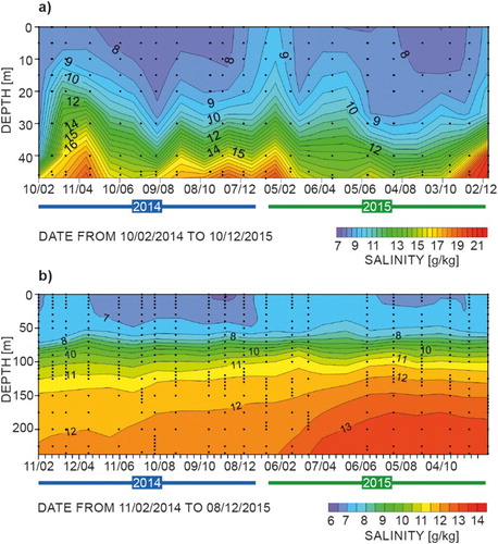
The MBI of December 2014 reached the Gotland Basin in March 2015 (Figure 44(b)). There, the impact of the MBI on ecological conditions in the deep layer is most crucial. MBIs bring oxygen-rich water to the Baltic and the anoxic water in the Gotland Basin is replaced with oxic water. Mohrholz et al. (2015) suggest that the total amount of oxygen transported into the Baltic is three times greater than the oxygen equivalent of hydrogen sulphide found in the Gotland Basin in November 2014 (Schmidt 2014). At first, the nutrient conditions in the Gotland Basin react to the inflow – ammonium is oxidised and phosphate is fixed in the sediments. A decrease in phosphate concentration occurred in the Gotland Basin in 2015 (not shown). Water with salinity in excess of 12.5 g/kg fills the approximately 100 m thick bottom layer (depth range between 150 and 250 m) in the Gotland Basin (Figure 44(b)). High bottom salinity of about 13.5 g/kg is observed until the end of 2015 at least. It should be further noted that there was an increase in salinity in the Arkona Basin in November–December 2015 (Figure 44(a)), which may indicate further replenishment of the Baltic Sea deep basins with oxygen-rich water.

3.5. Iberian-Biscay-Irish Sea

Leading authors: M.G. Sotillo, B. Levier, A. Pascual

Contributing author: Antonio Gónzalez Ramos

The IBI area (see Figure 45) is a complex dynamic region with a remarkable variety of ocean physical processes and scales involved (Sotillo et al. 2015). Among other dynamic features, the IBI region presents a strong summer seasonal coastal upwelling conditions along the western Iberian and African continental shelves. In this first OSR, the IBI regional contribution focused on these IBI coastal upwelling processes due to the importance of this regional feature on the marine environment, carbon cycles and fisheries, and the noticeable social impacts linked to its climate variability. Coastal upwelling processes occur along the IBI coastlines as the result of deflection of the oceanic water away from the shore. Such deflection is produced by Ekman transport induced by persistent north trade winds blowing parallel to the coast line. When this transported water is forced, the mass balance is maintained by pumping of ascending intermediate water (Sverdrup 1938). This water is typically denser, cooler and richer in nutrients. Therefore, upwelled water can distinctively be identified by seasonally variable low SST and nutrient-rich water in coastal areas, compared to the averaged values at the same latitude. These specific properties of surface water on upwelling areas induce relevant impacts on coastal climate and marine biology (Miranda et al. 2012). The high primary productivity of coastal upwelling systems sustains large fisheries, meaning these areas are of great interest from an economic point of view where around 20% of the global fish production is concentrated on upwelling areas, which accounts for approximately only 3% of total ocean surface (Ryther 1969; Cushing 1971; Pauly & Christensen 1995; Fréon et al. 2009). The IBI contains two Eastern Boundary Upwelling Ecosystems (EBUEs). Both EBUEs are well-documented and hosted under the same system known as the Canary Current Upwelling System. The NW African continental shelf (NWA) presents three adjacent upwelling regions that extend from Morocco (34°N) to Southern Senegal (11°N). The West Iberian coastal shelf also has a homogeneous seasonal upwelling system (Fraga 1981; Botas et al. 1990; Borja et al. 1996, 2008; Bode et al. 2002; Alvarez et al. 2010) (Figure 46).

Figure 45. Schematic description of main IBI oceanographic features (Figure from Sotillo et al. 2015).

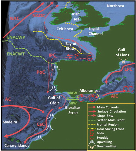
Figure 46. (a) August SST climatology derived from the IBI Reanalysis product (reference period: 2002–2014). (b) Surface Zonal Velocity (positive values not shaded): August climatology derived from IBI Reanalysis (reference period: 2002–2014) (bc) and (c) monthly field for August 2015 from the IBI operational near-real-time Forecast Service (cd). See text for more details on data use.

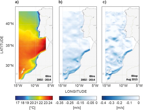
A classic way of quantifying upwelling intensity is by computing the Coriolis forces that induce the cross-shore Ekman transport. The wind-derived Coastal Upwelling Index (CUI) can be interpreted as the water flux theoretically transported offshore by the wind stress from the coast assuming an infinite ocean (Ekman 1905). Consequently, this CUI does not consider the bathymetry of the continental shelf. The surface cooling, from upwelled water reaching the sea surface, is also a potential proxy of the upwelling intensity. Therefore, CUIs based on comparisons between coastal and open-ocean SST at each latitude are widely applied to data provided by multisource data sets (remote sensing and models, Alvarez et al. 2010; Benazzouz, Mordanea et al. 2014; Cropper et al. 2014).

The IBI Monitoring and Forecast Centre (IBI-MFC) produces near-real-time and reanalysis products widely validated in literature (Maraldi et al. 2013; Sotillo et al. 2014; Aznar et al. 2016; Lorente et al. 2016). Both products, hereafter named IBIop²¹ and IBIre,²² respectively, were used to monitor the intensity of the offshore transport related to the upwelling process. As can be seen in Figure 46(a), both upwelling regions, African and Iberian, are clearly identified through their relative lower SST signals according to the CMEMS IBI model reanalysis data. Figure 46(c) illustrates the surface offshore transport, showing its maximum intensity along the African coasts (observed in the means of the climatological zonal velocity derived from The IBI reanalysis data for August). The use of the zonal velocity component as an approximation of the offshore movements may result in some underrepresentation of these water movements in some coastal spots, particularly those where the coastline is not aligned in the meridional direction. In order to allow some comparison between the last year available (2015) and the reference reanalysis period considered (2002–2014), Figure 46(c) shows the IBI surface zonal component current averaged for August 2015. Since IBI reanalysis was only run until 2014, the monthly zonal velocity field was derived from the CMEMS IBI-MFC near-real-time model system.

In order to monitor coastal upwelling conditions in the IBI area, two different upwelling indexes were computed. The first index, the CUI_EK, is based on the estimation of Ekman transport perpendicular to the shoreline. It is derived from the wind stress forcing (Bakun 1973). The surface wind data used to compute the CUI_EK are those used as atmospheric forcing of the CMEMS IBI reanalysis (ERA-Interim). A second upwelling index based on SST (CUI_SST) was also derived from each latitudinal point computing the thermal differences between the shelf and the open ocean. The CUI_SST computed at each latitude was defined as the temperature difference between the maximum and minimum temperatures in a range of distance from the coast up to 3.5° westward.

The CUI_EK and CUI_SST indexes were calculated along the NWA and the Iberian Peninsula (IP) coasts. Figure 47 displays the time series of the CUI_EK upwelling index at 30°N and 42°N. The higher index record represents the most intense upwelling conditions in each location. Strong seasonal variability is found in both cases; however in the NWA case (Figure 47(b)) the CUI_EK index values were much higher than in the IP western upwelling (Figure 47(a)). The African case, with positive index values almost all year round, indicated an almost constant upwelling in the NWA shelf, whereas in the Iberian case it was mainly observed in summer (very low and even negative index values very frequently during winter). The differences were related to the fact that the Iberian and African upwelling regions differed as to type of winds responsible for the transports: The IP upwelling winds were produced by the influence of the Azores High. These anti-cyclonic conditions were far from homogeneous, leading to remarkable seasonality of the upwelling process. Therefore coastal upwelling events occurred in the IP coast mainly during the spring-summer months (consistent with the literature; Alvarez et al. 2008, 2010). On the contrary, the upwelling conditions on the African coast were influenced by the northeast trade winds, as part of the lower pressure levels of the Hadley circulation cell. This atmospheric pattern was sustained all year long, and the associated wind regime on the African coast produced upwelling conditions from quasi-permanent to permanent (Cropper et al. 2014).

Figure 47. IBI CUIs: (a) and (b) Time series of CUIEK at 42°N (Western IP coast) and 30°N (NWA coast), respectively. CUIEK Index derived from estimation of Ekman transport perpendicular to shoreline of atmospheric forcing of the CMEMS IBI reanalysis. (c) CUISST, zonal Hovmöller diagram. CUISST Index derived from the CMEMS IBI reanalysis data for the 2002–2014 period and from the CMEMS IBI Forecast & Analysis service for the year 2015 (see text for more details on data use). The vertical black line limits the use of both datasets. White horizontal dashed lines denote the latitudes 42°N and 30°N, where CUIEK time series are shown in panels (a) and (b).

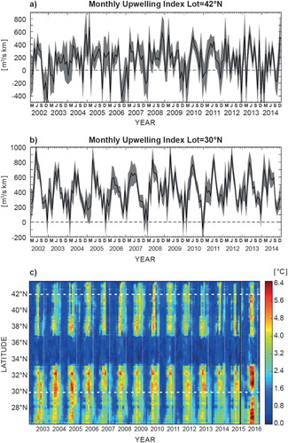
Additionally, a CUI_SST index, based on oceanographic data (SST fields), was computed along the IBI coasts using both the CMEMS IBI reanalysis (reference period: 2002–2014) and the near-real-time operational ocean forecast system (latest year: 2015). The results from both IBI products are shown together in Figure 47(c). It is worth mentioning that both products come from different model solutions and therefore are not comparable. However, there are some consistencies between them where they present similar seasonality in 2015 compared to the period 2002–2014.Further information on the consistency between the IBIop and IBIre products can be found in Aznar et al. (2016). Examining the CUI_SST values along latitude and time shows a significantly different upwelling intensity in NWA and IP. During the complete time record the index values in NWA usually presented thermal differences (> 4°C) while on the IP coast, such thermal gradients occurred during specific summer seasons. Attending to the CUI_SST temporal evolution, the NWA coast showed a quite constant variability of the periodicity and the intensity of the upwelling. On the contrary, in the IP region (2004–2009 years), the results showed an intensification of the coastal thermal gradients during the summer upwelling season (higher CIU_SST maxima) and aside from the years 2002–2003 and 2010–2014 the CUI_SST presented lower maxima. The weaker signal found in the IP region throughout the years 2012–2014 was also identified by both indexes (the CUI_SST and the CUI_EK at 42°N) affecting most of the Iberian coastal areas, but not the NWA region. The results obtained by the CUI_EK and CUI_SST indexes showed the clear existence of a lag (1–2 months) between the annual distribution of CUI_Ek (Figure 48(a)) and the CUI_SST (Figure 48(b)). This lag has also been observed in previous studies (Fiuza et al. 1982; Nykjaer & Van Camp 1994; Castro et al. 2008; Alvarez et al. 2010; Cropper et al. 2014) and it may seem quite long compared to the rapid response (time scale of a few days) of the coastal ocean to changes in local wind forcing. However, it is explained due to the dynamic connection between adjacent areas induced by the along shore momentum advection. Consequently, the entire upwelling region marches in unison, introducing a seasonal memory to the system in accordance with the atmospheric-forcing annual cycle (Benazzouz, Pelegrí et al. 2014).

Figure 48. Averaged monthly CUIek (a) and CUISST (b) indexes, contoured by latitude and month. Reference period: 2002–2014 (the CMEMS IBI reanalysis time coverage). Grey horizontal dashed lines denote the latitudes 42°N and 30°N, where CUIEK time series are shown.

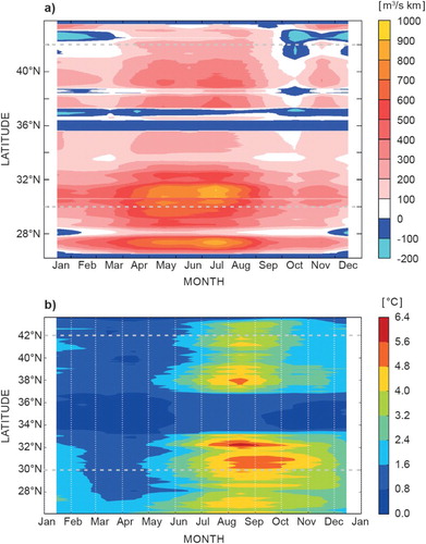
The effect of the coastline orientation and bathymetry also affected both indexes, appearing as a significant reduction in the CUIs signals at 28°–30°N, where the existence of the Canary Islands Archipelago induces a net reduction of the upwelling indexes and the inhibition in the interannual variability.

Chapter 4: Specific events

The ocean plays a pivotal role in the Earth’s physical, geochemical and biological systems and as such affects us all in pervasive and profound ways. This is particularly the case for specific unusual and severe events taking place in the marine environment that can have large – even worldwide – impacts on society. Through CMEMS, marine high-quality core data are available providing the opportunity for more and better-coordinated efforts in the observing of and understanding of such events that are taking place around the globe. This allows the challenge of delivering useful ocean information for societal benefits to be addressed. In this chapter, four phenomena are focused upon that have appeared to be unusual during the year 2015. Occurrence and intensity of these events are discussed, with regard to past events. The 2015 El Niño event is chosen first. This worldwide impact phenomenon has been greatly discussed, and it is considered important to provide its description based on the CMEMS integrated monitoring approach. A focus on the North Atlantic cold event that may have an impact on the regional climate changes over Europe is also provided. Both phenomena are discussed relative to the past, based on monitoring over the two last decades from CMEMS products. Two severe phenomena are also highlighted that may potentially result in severe consequences to the European coasts and in European waters. These are harmful algae blooms (HABs) in the Baltic Sea, and storm surges and extreme sea levels at the European coasts. The objective here is to offer an overview of occurrences and extreme values in 2015 relative to previous years. The monitoring of these events should be regularly highlighted, and will be extended to other potentially damaging phenomena in future reports.

4.1. The 2015 El Niño event

Leading authors: Marie Drévillon, Magdalena Balmaseda and Florent Gasparin

Contributing authors: Karina von Schuckmann, Eric Greiner

The most striking event of 2015 in the global ocean was the occurrence of a very strong El Niño in the Tropical Pacific (McPhaden 2015; Schiermeier 2015). In the ocean, El Niño is first characterised by a strong warming of surface and subsurface waters from the central Pacific to the coasts of Peru and Ecuador (see for instance the review by Wang & Picaut 2004). This warming is one of the main features of the 2015 annual mean SST anomaly (see Section 1.1). The 2015/2016 El Niño also displays a very strong signature in all EOVs (Chapter 1). The surface warming is only one of the manifestations of an ocean/atmosphere interaction that moves huge amounts of energy across the whole tropical belt, disrupts Tropical Pacific oceanic winds and currents (see Section 1.6), induces regional changes in sea level (Section 1.4) and impacts the atmospheric general circulation at the global scale. Impacts include: regionally intense precipitations, increasing the risk of flood, or exceptional droughts, and increasing the risk of wildfires. For instance, severe droughts occurred in Australia and Indonesia in 2015 related to this El Niño event. Last, but not least, warm El Niño Southern Oscillation (ENSO) events significantly slow the primary production at the Tropical Pacific basin scale, related to the cut-off of nutrient inputs from coastal and equatorial upwelling (Thomas et al. 2012, see Section 1.5). ENSO has been extensively studied and monitored thanks to the Tropical Atmosphere Ocean (TAO) Triangle Trans-Ocean Buoy Network (TRITON) (TAO/TRITON) (McPhaden et al. 1998), which gives the necessary subsurface information complementing satellite SST and SLA observations (the latter being also a proxy for heat content). Since 2005, the ARGO profiles give a precious complement to the TAO buoy records, which unfortunately have suffered from degradation over the past few years. The ocean 3D analyses or reanalyses – assimilating all these observations into numerical models – are not only providing ocean initial conditions for coupled ocean–atmosphere ENSO forecasts, but are also additional tools to study ENSO processes and provide unique hindsight of past events (see for instance McPhaden et al. 2015). An overview of how the 2015 El Niño event is captured by global ocean reanalyses such as the CMEMS global reanalysis product GLORYS (GLobal Ocean ReanalYsis and Simulation) (see Section 1.6, endnote 13), and C3S ORAS4 (Ocean Reanalysis System 4 as in Balmaseda, Mogensen, et al. 2013) is provided here. The latter has coarser horizontal resolution of 1° but with a 0.3° refinement at the equator, and spans a longer time period (1958 to present). The robustness of the following analysis is ensured by the independent validation of GLORYS and ORAS4 and by the consistency that can be observed in between these different monitoring systems’ results in the Tropical Pacific (Balmaseda et al. 2015).

Figure 49(a) shows the remarkable strength of the 2015/2016 phenomenon, which is comparable to the 1997/1998 El Niño in terms of surface temperature anomalies, with more than 2.5°C average anomaly at the surface in the nino3.4 box at the peak of the event in December 2015. The monthly SST anomalies reached 6°C at the surface locally (not shown). The 2015 sea surface salinity (SSS) is marked by a large freshwater anomaly whose extensive spatial scale and large amplitude have not previously been captured over the last two decades. While positive SSS anomalies are found in the far Western Pacific, large fresh anomalies extend over the Central-Eastern Pacific at the sea surface (Figure 49(b)), but also in the subsurface (see also Section 1.3). This large freshwater anomaly results from increased precipitation, related to the eastward displacement of the main atmospheric convection zone over large SST and heat content anomalies (Figure 49(b)), and from zonal advection changes, as can be induced by the surface currents (Section 1.6, Figure 19(b)). The 2015 characteristics combine both Central and Eastern Pacific El Niños typical patterns (Capotondi et al. 2015), including typical salinity-related patterns (Gasparin & Roemmich 2016). Using oceanic observations and atmospheric reanalyses, Gasparin and Roemmich (2016) concluded that the 2015 freshwater anomaly causes a positive steric height anomaly in the western Pacific, and significantly increases eastward surface acceleration at the SSS front due to the zonal pressure gradient.

Figure 49 (a): Monthly SST average anomaly (°C, black line and colour shading) in the nino3.4 box (as shown by the white rectangle in b) from the Mercator Ocean monitoring system, with respect to the GLORYS (see Section 1.6, endnote 13) 1993–2014 climatology. (b): December 2015 average anomaly of heat content in the 0–300 m layer (GJ/m²) from the Mercator Ocean monitoring system with respect to GLORYS (1993–2014) December climatology. (c): Annual 2015 average of surface salinity anomaly SSS (psu) in the Tropical Pacific from the Mercator Ocean monitoring system with respect to GLORYS (1993–2014) climatology.

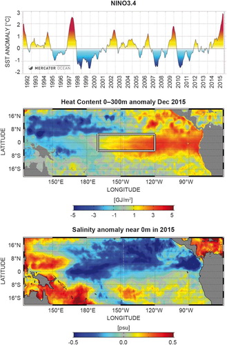
The El Niño warming affects the subsurface layers of the ocean, and has a strong imprint in upper OHC anomalies (Figure 49(c), see also Section 2.1): a huge amount of heat is moved from the west to the east of the basin. Part of it is vented into the atmosphere (by affecting the patterns of organised atmospheric convection and by fueling strong hurricane activity), and part of it continues recirculating adiabatically around the Pacific basin. The patterns of the upper OHC anomaly are well matched by sea level.

The time evolution and onset of the 2015/2016 El Niño can be seen in Figure 50(a). Strong westerly wind bursts (WWBs) during the 2015 winter triggered a series of downwelling Kelvin waves (Figure 50(b)), which propagated east and reached the eastern part of the basin in April 2015. The resulting flattened thermocline over the Equatorial Pacific (Figure 50(b)) and reduced upwelling were responsible for the development of a large SST anomaly in the eastern part of the basin, which strengthened and propagated westward. The WWBs also contributed to push eastwards the edge of the warm pool, as indicated by the slowly eastward propagating SST anomalies around the dateline. The SST anomaly in the Central Pacific reached its peak at the end of 2015 (Figure 50(c)). As can be seen in Figure 50(a), WWBs also took place at the beginning of 2014, which also triggered strong Kelvin waves, caused some warming in the east of the basin and displaced the warm pool. But these perturbations were insufficient to trigger El Niño. Instead, an easterly wind burst (EWB) took place at the beginning of July that terminated the incipient warming. Levine and McPhaden (2016) discuss how this EWB was instrumental in enhancing equatorial warm water volume, the EWB setting the scene for the occurrence of the strong 2015/2016 El Niño event one and a half years later.

Figure 50. Longitude–time diagrams (October 2013 to October 2015) from the ocean reanalysis system ORAS4 (Balmaseda, Mogensen, et al. 2013) It should be noted that an updated version of this reanalysis will be part of CMEMS in the near future. (a) zonal wind stress at the Equator (m/s), (b) depth of the 20°C isotherm at the Equator and (c) SST. The anomalies are with respect to the 1981–2009 climatology.

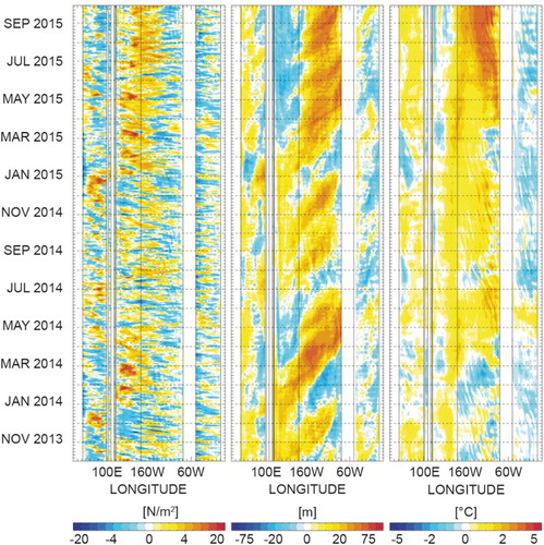
4.2. The recent North Atlantic cold event

Leading authors: Fabrice Hernandez, Karina von Schuckmann, Clotilde Dubois

Contributing authors: Charles Desportes, Joaquin Tintoré, Melanie Juza, Stéphanie Guinehut and Jerome Gourrion

Although the global Earth’s 2015 surface temperatures were the warmest since modern record keeping began in 1880 (NASA 2016), a particularly strong cold signature was observed in the North Atlantic Ocean. Using the global CMEMS ocean reanalysis GLORYS (see Section 1.6, endnote 13) in order to analyse dynamically consistent patterns, this signature appears located poleward of the North Atlantic Current (NAC) system up to the northern fronts of the subpolar gyre, approximately in a domain limited from 40°W to 15°W, and 48°N to 60°N (Figures 51 and 52). Anomalous cold SSTs have also been recorded since the 2013 boreal winter in this region (e.g. Josey et al. 2015), where it is observed that temperature anomalies exhibit the largest maxima during the second half of 2015, with values larger than 3°C near the surface. This cold-water anomaly signature extends at depth down to 1200 m. From the surface down to 500 m, it exceeds 3°C at 48.7°N/27.5°W in November 2015 (Figure 52). In comparison, the seasonal cycle amplitude never exceeds 0.5°C below 200 m in this above-mentioned domain. The whole anomaly extends slightly towards the north-east during 2015, associated to a constant deepening around 55°N, between 40° and 20°W that reaches more than 800 m deep. Associated with this temperature anomaly, the model salinity field presents a similar pattern, at the same time and within the same area, with anomalous freshening far beyond the typical amplitude of the seasonal cycle (Figure 52). Fresher waters larger than 0.5 PSU are seen to follow the maximum of the temperature anomalies. At depth, a deepening of this salinity-negative pattern also appears, although extending less deep, with anomalous signature larger than 0.2 psu limited to the first 700 m (Figure 52). Both temperature and salinity anomalies are also recorded through the global analysis performed at Sections 1.2 and 1.3, based on a different CMEMS global product.

Figure 51. Annual mean regional OHC (0–700 m) anomaly for 2015. Based on monthly averages of the CMEMS ¼° global daily reanalysis GLORYS (see Section 1.6, endnote 13). Anomalies are relative to the climatology over 1993–2014 from the reanalysis. Units are in gigaJ/m². The yellow dot corresponds to the location of the virtual mooring presented in Figure 52.

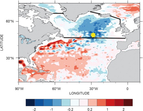
Figure 52. Left panel: Time series diagram of a virtual mooring from 0 to 2000m depth at 48.7°N/27.5°W (see Figure 51) over 2012–2015 of temperature (shaded, in °C) and salinity anomalies (thick contours, every 0.1 PSU, for negative anomalies). The stamped map in the bottom left corner of the diagram gives the position (red dot) of this virtual mooring plot. Monthly averages of the CMEMS ¼° global daily CMEMS reanalysis product GLORYS (see Section 1.6, endnote 13) are used. Anomalies are relative to the monthly climatology over 1993–2014 from the reanalysis. Right panel: For each depth corresponding to this virtual mooring time series, the temperature anomaly minimum (black) and maximum (red) are plotted, together with the absolute amplitude of the seasonal cycle (orange), as derived from the reanalysis monthly climatology. Depth of the min/max values are indicated.

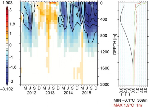
Besides its global uniqueness in intensity, this cold pattern is located in an ocean area of particular importance (Figure 51). Changes in this area are driven by several processes: (1) the physical interactions at the atmosphere–ocean interface controlling heat and momentum transfer; (2) the internal ocean dynamic processes such as the AMOC controlling the global ocean climate at decadal and longer time scales; (3) the wind-driven circulation changes of the major ocean gyre systems; and (4) the formation of new water masses connecting the two through its exchange mechanisms between the surface and deep ocean and ventilating and renewing water layers of the interior ocean (see Section 2.3). Moreover, this area can be affected by freshwater inflow from ice melting processes in the Arctic, which in turn induce changes in the North Atlantic density field. The interplay of different physical processes in this area is very likely modulating climate variability, in particular over the European continent and North America (Marshall et al. 2001).

So how has this pattern emerged? This is still a matter of current research and discussion. Air–sea interaction might be one of the main causes. This is supported by anomalous recorded SST and near-surface winds in the area that control the rates of heat and momentum transfer between ocean and atmosphere. Latent heat fluxes forcing the CMEMS ocean reanalysis exhibit anomalous loss during the successive winters of 2013/14 and 2014/15. During these winters, the North Atlantic mid- and high-latitude air–sea heat exchange was dominated by anomalously strong north-westerly winds, bringing exceptionally cold and dry air across the Northeast Atlantic (Grist et al. 2016). In particular, recent studies have identified that this cold pattern is part of interannual to decadal variability through its connection to climate modes such as the EAP and the NAO (Robson et al. 2012; Yeager et al. 2012; Josey et al. 2015), affecting also deeper layers of the North Atlantic (Häkkinen et al. 2015).

In particular, these severe winter heat losses were remarkable in size in the Labrador Sea and across the mid- and high-latitude North Atlantic. They left a major imprint on ocean properties both at the surface and at depth. The OHC (Section 2.1) of the sub-polar gyre region has decreased during the last decade (Figure 53, Häkkinen et al. 2015). This change in local heat storage can in turn affect the winter’s air–sea exchange on ocean and atmospheric transport pathways, as well as regional sea level patterns through thermosteric effects (see Section 1.4). Moreover, the cooling to depth (Figures 52 and 53) on the poleward flank of the NAC has led to increasing zonal geostrophic flow associated with the NAC (Grist et al. 2016).

Figure 53. Area of mean OHC (0–700 m) anomaly in J/m² averaged between 45°N and 65°N (see limits in Figure 51) in the Atlantic Ocean over the last two decades. The annual mean values obtained from the in situ observing system (red curve, see Section 2.1, endnote 17) are superimposed on monthly mean values using the CMEMS ¼° model products used in Figure 51 (see also Section 1.6, endnote 13). Uncertainty estimates on the observed OHC changes are detailed in von Schuckmann et al. (2009).

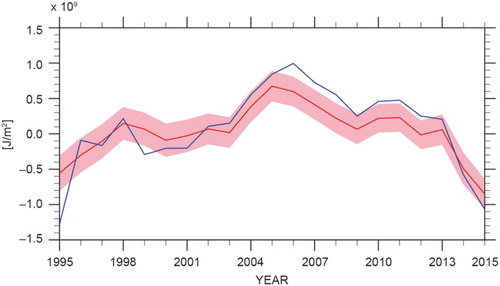
It has been proposed that one of the most important links to the North Atlantic cold event was related to most intense formation of deep water (Labrador Sea Water, LSW) of the early twenty-first century (Kieke & Yashayaev 2015). Labrador Sea wintertime mixed-layer depths in 2013/14 exceeded 1700m, delineating a reservoir filled with a newly ventilated (hence rich in CO₂ and other dissolved gases), cold and fairly fresh LSW. Modelled mixed layers are also particularly deep during the winter 2015 all along the 45°–60°N latitude band, from to 55° to 10°W, in particular at the boundaries of the Labrador Sea, where a mixed layer deeper than 1800m appears in March 2015 at 50°W/58°N. Such modelled deep mixed layer events, both in the Irminger and Labrador Seas, only appear in the reanalysis records in the early 1990s (Figure 53). Moreover, independent analyses indicate that freshwater fluxes from Greenland have also contributed to changes in LSW (Yang et al. 2016), and are linked to AMOC strength (Brunnabend et al. 2015; Yeager et al. 2015; Yang et al. 2016).

However, the question of whether the Atlantic cold event is linked to Atlantic Multi-decadal variability, as well as to the AMOC system, is at the periphery of current climate research. Many studies are now predicting a cooling of the North Atlantic (Hermanson et al. 2014; Klöwer et al. 2014; Robson et al. 2014) and the key questions are if, and when, the North Atlantic will enter a cold phase. As discussed above, simultaneous changes in atmospheric circulation contributed to this cooling pattern at seasonal to interannual time scales, but it is also suggested that they cannot fully explain the cooling, suggesting that ocean circulation changes at decadal time scales are an important forcing factor (Smeed et al. 2014; Robson et al. 2014; Rahmstorf et al. 2015; Yeager et al. 2015).

4.3. Harmful algae blooms in the Baltic Sea in 2015

Leading authors: Bengt Karlson, Lena Viktorsson

Harmful algal blooms have a global distribution and can have impacts on marine ecosystems, fisheries, aquaculture and tourism. There are at least four main types of harmful algal blooms, (1) blooms of algae-producing biotoxins that may accumulate in shellfish such as mussels; (2) blooms of fish-killing algae causing problems for fisheries and aquaculture; (3) blooms of algae that are a nuisance due to their accumulation on beaches etc.; and (4) ecosystem-disruptive blooms, e.g. the bloom of Prymnesium polylepis (syn. Chrysochromulina polylepis) in Scandinavia in 1988. In addition, blooms of benthic microalgae-producing toxins that are found in aerosols from ocean spray may be a problem for human health. The frequency and distribution of harmful algal blooms may be increasing (Hallegraeff 1993) and climate change will affect these blooms (Wells et al. 2015). High-biomass blooms may also lead to anoxia in deep water in cases where grazers do not limit biomass build-up. Here, blooms of diazotrophic (nitrogen fixing) cyanobacteria in the Baltic Sea are focused upon. These cyanobacteria blooms have a high biomass and may be detected using automated methods.

Accumulations of cyanobacteria in surface waters are common in the Baltic Sea during July and August and are visible on satellite images. These blooms mainly include Nodularia spumigena, Aphanizomenon sp. and Dolichospermum spp. and are considered a major environmental problem in the Baltic Sea. N. spumigena produces the hepatotoxin nodularin. Large surface accumulations at sea and on beaches cause a loss of recreational value and also add considerable amounts of biologically available nitrogen to the system through nitrogen fixation. Due to increased eutrophication of the Baltic Sea there have also been concerns that this could lead to an increased frequency in cyanobacteria blooms also increasing deep water anoxia (Vahtera et al. 2007). To be able to monitor the development of cyanobacteria blooms and detect changes in frequency and coverage of the blooms, a combination of satellite observations and plankton sampling using research vessels and Ferrybox water sampling is used (Karlson et al. 2016). In addition, fluorescence from phycocyanin, a proxy for cyanobacterial biomass, is measured using oceanographic buoys and Ferrybox systems (Seppälä et al. 2007). Ferrybox data from the CMEMS regional near-real-time product²³ in 2015 collected using the merchant vessel TransPaper on the route Lübeck-Kemi-Oulu-Lübeck are presented in Figure 54. So far, a full evaluation of such a data set has not been performed for the Baltic Sea. Satellite data on ocean colour have been used to analyse both the frequency and coverage of the summer cyanobacterial blooms (e.g. Öberg 2015). By using a multi-decadal time series of satellite data from multiple sensors Kahru and Elmgren (2014) showed that there was a significantly higher areal fraction of cyanobacteria during 1997–2013 compared to the earlier period 1979–1996.

Figure 54. A Ferrybox system on the merchant vessel TransPaper was used to collect data continuously on the route Lübeck-Oulu-Kemi-Lübeck every week. Data were collected every 20 s. Results from June to September are presented. (A) Temperature, (B) Salinity, (C) Chlorophyll fluorescence, a proxy for total phytoplankton biomass and (D) Fluorescence from phycocyanin, a proxy for the biomass of phycocyanin-containg cyanobacteria. The map indicates the route of the ship in 2015. Red lines show the area from which data are presented.

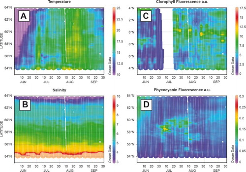
In most years, satellite observations of the blooms are made in July, while the cyanobacterial bloom in 2015 was mainly observed in August using satellite data. Ferrybox data on phycocyanin fluorescence indicate that there were large amounts of cyanobacteria in July and August. Thus satellite data may underestimate the coverage of the bloom. To monitor the extent of cyanobacterial blooms the Swedish Meteorological and Hydrological Institute (SMHI) uses a combination of in situ data and satellite data. To monitor cyanobacterial blooms a map that shows the number of days with observation of blooms (see Figure 55, Öberg 2015) is produced each year. These data show that 2015 is not a year with a strikingly high number of blooming days, but that blooming days were recorded from the Southern Bothnian Sea to the Bornholm, affecting most of the Baltic Sea basins. After Envisat became inoperative in April 2012, the SMHI used Aqua-MODIS satellite data on a daily basis during the summer months from June to August. In 2016, data from the NASA satellite Suomi-NPP have been added. Ocean colour data from the OLCI-sensor on ESA-Sentinel 3a will be added as soon as they are available operationally. The satellite was successfully launched in February 2016 and Sentinel 3b should follow 18 months later. The two Sentinels will provide two overflights per day which should make cloud cover less of a problem than at present.

Figure 55. Number of days of satellite observations of cyanobacteria surface accumulations in June–August 2010–2015. The observations are based on a combination of Aqua-MODIS (NASA, https://modis.gsfc.nasa.gov/) (2010–2015) and EnviSAT-MERIS (2010–2011, https://earth.esa.int), figure from Öberg (2015).

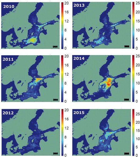
High-biomass blooms of cyanobacteria may be detected using ocean colour data from satellites during cloud-free conditions. CMEMS currently offers a chlorophyll-a and an SST algorithm for satellite data, but does not offer ocean colour data for the Baltic Sea at present. The data presented are from the SMHI-operated Baltic Algae Watch System and from a Ferrybox JERICO-NEXT project. The satellite data on cyanobacteria blooms are sensitive both to cloud cover and to wind conditions. Wind-induced turbulence causes surface accumulations of cyanobacteria which are mixed down in the water column. Ferrybox systems are useful for measuring optical properties of phytoplankton, in this case the fluorescence of the pigment phycocyanin. This is a very useful complement to the satellite measurement, both as a means to provide therminology for improving the ocean colour algorithm and to get more detailed knowledge on what type of plankton is in the water. Ferrybox systems are also used for automated collection of water samples that are analysed in the microscope or using imaging flow cytometry. This makes it possible to identify harmful species and to investigate plankton biodiversity.

4.4. Extreme sea level events

Leading authors: Begoña Pérez Gómez, Enrique Álvarez Fanjul, Jun She

Contributing authors: Irene Pérez González, Fernando Manzano Muñoz

The scientific community agrees on the rise of global mean sea level during the last century (Church & white 2011; Church et al. 2013; Hay et al. 2015). This sea level rise, possibly accelerated in the last few decades (Holgate & Woodworth 2004; Church et al. 2006; Araújo & Pugh 2008; Jevrejeva et al. 2008; Merrifield et al. 2009), may lead to greater impacts of storms on the coast through coastal flooding and/or damage to coastal infrastructure. Storm surges are generated by severe windstorms and their magnitude is larger for those basins with shallower waters such as the North Sea (Pugh 2004). Many studies have been published about long-term changes in storm surges and their geographic patterns worldwide, based on both tide gauge data and numerical models (Woodworth & Blackman 2002, 2004; Vilibić & Šepić 2010; Merrifield et al. 2013; Talke et al. 2014; Weisse et al. 2014; Cid et al. 2015; Wahl & Chambers 2015; Marcos et al. 2011, 2015 etc). The trends in storm surge are less clear than the ones in mean sea level, however. For example, according to Vilibić and Šepić (2010), the storminess and extremes trends are generally positive over Northern Europe and negative over Central and Southern Europe. There is no significant trend either in the storminess in the North Atlantic according to Dangendorf et al. (2014). Marcos et al. (2011) found a decrease in the projected number of positive storm surges and an increase in the number of negative surges in the Mediterranean throughout the twenty-first century. In the North Sea, the storminess was high at the end of the nineteenth century and subsequently declined until about 1960, followed by a strong upward trend until the mid-1990s. Since then, up until now, a return to average conditions is evident although in 2015 up to nine of these extreme storms were identified in this basin. In this section we analyze the variability of the surge component of the tide gauge data (tide extracted) available in CMEMS in situ data portals (see endnotes 24–26 for more details), for the period 1993–2015. The objective is to put 2015 storm surges in context and to explore possible trends on this surge component during the study period, while pointing out to the adequacy of sea level data available in CMEMS for this type of studies.

A first review of the sea level time series available in CMEMS showed diverse data sampling, with only about 18% of the stations providing data spanning from 1993 to 2015 and very few time series from the Mediterranean basin. For simplification, in this first report only those stations with validated hourly sampling data have been used. This has reduced significantly the number of stations (79). This number will increase in future reports when adequate standard data processing is applied to all the time series. This simplification, unfortunately, may bias the results when basin-wide results are presented, as now there is a lack in information from many tide gauges in the most important storm surge regions (e.g. the Netherlands, Germany or France). For the 79 stations available (displayed in Figures 56–58) tidal constants, tide prediction and surge component (hourly sea level – hourly tide) were computed. The latter, analysed and presented here, represents mainly atmospherically forced components of sea level (atmospheric pressure and wind), providing information on storm surge events and storm variability. The final impact of these at the coast (total sea level) is not addressed here and depends locally on the final combination of the local tide and this surge component (as well as other higher-frequency phenomena such as ‘seiches’ or meteotsunamis with periods of several minutes, not present in filtered hourly data).

Figure 56. (a) 99th percentile annual level of hourly surge data for each tide gauge in the IBI region; large circles: 99th percentile for 2015 mean value at each station for the period 1993–2014, inner smaller diamonds: mean value at each station for the period 1993–2014. (b) evolution of the 99th (top) and first (bottom) annual percentile levels of hourly surge data averaged for all the stations in the IBI region: black lines: averaged value and standard deviation for each year; magenta lines: maximum and minimum values in the whole region for each year. See endnote 24 for more details on data use.

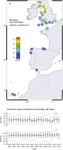
Figure 57. (a) 99th percentile annual levels of hourly surge data, for each tide gauge in the NWS region: large circles: 99th percentile for 2015, inner smaller diamonds: 99th percentile for 2015. (b) evolution of the 99th (top) and 1st (bottom) annual percentile levels of hourly surge data averaged for all the stations in the NWS region: black lines: averaged value and standard deviation for each year; magenta lines: maximum and minimum values in the whole region for each year. See endnote 25 for more details on data use.

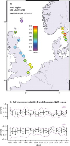
Figure 58. (a) 99th percentile annual levels of hourly surge data for each tide gauge in the BAL region: large circles: 99th percentile levels for 2015, inner smaller diamond: mean value at each station for the period 1993–2014. (b) evolution of the 99th (top) and 1st (bottom) annual percentiles of hourly surge data averaged for all the stations in the BAL region: black lines: averaged value and standard deviation for each year; magenta lines: maximum and minimum values in the whole region for each year. See endnote 26 for more details on data use.

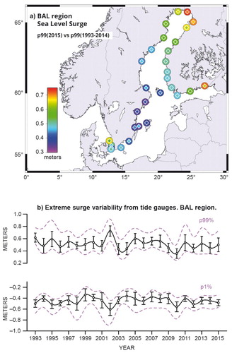
The percentile time series analysis approach of Woodworth and Blackman (2004) is followed for assessment of the extremes variability of the surge component during the study period. This method determines changes in the frequency distribution of measured sea levels. Different percentiles were computed annually for each station, for those years with data completeness over 70%. The 99th and the 1st percentiles will represent approximately the levels of the 1% highest and lowest hourly levels, respectively, for each year (top and bottom parts of the distribution of hourly levels). The 99th percentile of year 2015 is displayed along with the 1993–2014 mean value for each station in the following regions: Iberian-Biscay-Ireland coast (IBI), North Sea (NWS) and Baltic Sea (BAL) (Figure 56–58, maps on the upper panels). The 99th percentile (higher extremes) and the 1st percentile (lower extremes) were spatially averaged regionally and the temporal evolution displayed on the bottom panels of the same figures. As the annual mean sea level and the tide have been subtracted, the long-term mean sea level trend effect is not present in this analysis.

According to the hourly data available in CMEMS for this period it can be seen that the range of variability of the surge component, spatially averaged, goes from around −0.9 m to 1.0 m in the three regions of study. In addition, the averaged surge component of sea level in 2015 was not generally larger than the values from previous years.

The IBI region is the one with the largest spatial variability due to the stations located at lower latitudes, where storms are less frequent, but also where the amplification effect of shallow waters is smaller (Iberian Peninsula and, mainly, the Canary Islands). Here, along the European Atlantic coast, the 99th percentile surge in 2015 (p99–2015) ranged from about 0.2 m at the Canary Islands to 0.85 m in the Bristol Channel and the Irish Sea (Heysham, UK). In comparison to the period 1993–2014, however, most of the stations did not present larger extremes in 2015; the p99–2015 was only clearly larger (notice the different colours between the inner diamond and the external circle) at the northern part of the Irish Sea, in the UK. In the NWS region, the p99–2015 ranged from 0.50 m to 0.75 m (maximum value in Stenungsund, Sweden). The lowest value was clearly less negative than in the IBI region, as expected for these higher latitudes and the shallower depths (wide continental shelf) of the North Sea. Nevertheless, in 2015 the larger positive surge values appeared on the Western Atlantic coast of the UK (displayed in the IBI map), as mentioned above. The map in Figure 57 shows that the extremes were larger in 2015 for the Scottish stations and along the Western coast of Sweden. In the Baltic, the p99–2015 ranged from 0.35 m to 0.75 m, with the largest values found in the northern part of the Gulf of Bothnia and in the Gulf of Finland. Interestingly, the values were larger at the eastern stations (Finland coast) than at the western stations (Sweden coast). The extremes in 2015 did not change or were even smaller, however, in the whole BAL region.

From the spatially averaged time series in Figures 56–58, the largest interannual variability of these extremes appeared in the Baltic Sea while, as already mentioned, the IBI region presented the largest spatial variability (magenta curves in the Fig.). Another interesting feature is that the surge component of sea level in 2015 was not generally larger than the values recorded in previous years. A significant trend in the evolution of these percentiles over the last two decades is not present either, which is coherent with recent publications (e.g. Dangendorf et al. 2014 and others). In spite of this general conclusion for the region, it is important to bear in mind that the contribution of the long-term mean sea level evolution and even of the nodal tide might lead to largest (or lowest) total sea levels in practice; these total sea level extremes would nevertheless not be caused by enhanced meteorological forcing, according to this study, which will be supplemented when more stations become available. This seems in contradiction to the statement in the introduction about the increased number of severe storms in Europe for the last few years; this should be confirmed with a study of the frequency of extreme events from the tide gauge records, not included here (as for example in Cid et al. 2015; Marcos et al. 2015). The frequent storms occurring in 2015 caused inflow events to the Baltic Sea and several large local storm surges. For example, six storms hit Denmark in 2015, including one hurricane-like storm named Gorm with a maximum wind speed of 45.9 m/s. All these storms came from the west. In the past 100 years, only 1921 had more storms (7) than 2015 in this country. The link between this increased frequency and climate change (e.g. a southward shift of the storm track) is not clear. The storms also caused surges on the west coast as well as in the fjords (e.g. Limfjorden) in Denmark.

Concerning the adequacy of sea level time series available in CMEMS, it has become evident that there is a need for establishing homogeneous requirements on data sampling within CMEMS in order to avoid the diverse sampling intervals along the same time series. This is important because different physical processes can be adequately resolved with these different sampling strategies. On the other hand, it was found that only about 18% of the stations had data spanning 1993–2015 and that many existing stations were not yet available in the service. All these issues will be discussed in detail in future.

Chapter 5. Synthesis

Principal findings of this first CMEMS OSR 2016 can be categorised in two main synthesis messages. The first one is related to decadal scale changes during the period 1993–2015. It relies on evaluations presented in Chapters 1 and 2. These results can be summarised as follows (see also Figure 59):

• A decadal scale sea level rise is clearly observed at global scale, in the Mediterranean Sea, the North-West Shelf, the IBI Seas and in the Black Sea. Decadal scale sea level rise for the latter two regions is of comparable size as global scale changes, whereas the other two regions show slightly lower sea level rise compared to the global values (Section 1.4).

• Ocean thermal expansion (volume changes) accounts for about 30% of the decadal sea level rise at global scale and between 30 and 50% for the Mediterranean Sea, in the North-West Shelf, and in the IBI area (Section 1.4).

• An OHC increase is observed at global scale and in the Mediterranean Sea, the North-West Shelf and the IBI area. The ocean heat increase is somewhat higher than the global one in these three European regions (Section 2.1).

• An increase in SST is observed at global scale. At regional scale in the Mediterranean Sea and in the Black Sea, the SST increase is significantly higher (Section 1.1).

• A significant decrease in Arctic sea ice extent occurs at decadal scale (a decline up to 15.8% per decade during summer), whereas a significant increase in Antarctic sea ice extent is reported (Section 1.7).

  Figure 59. Overview on decadal scale changes during the period 1993–2015 as obtained from the first CMEMS OSR 2016. The flash icons indicate increasing or decreasing decadal trends for the different physical parameters, which have been evaluated for the global ocean (GLOB), and for specific regions whenever possible such as the Mediterranean Sea (MED), the IBI Sea, the North-West-Shelf (NWS) and Black Sea (BS), see Figure 1. Information on uncertainty estimates can be found in the corresponding sections.

  

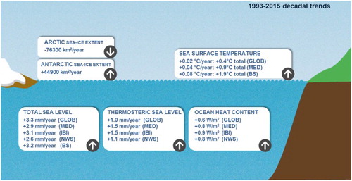
The second key synthetic information is related to the monitoring of anomalous changes during the year 2015, referenced to a baseline climatology over the period 1993–2014, in particular (see also Figure 60):

• Exceptionally strong sea surface temperatures occurred in the entire Northern hemisphere (Section 1.1).

• One of the lowest Arctic summer sea ice extent ever measured over the past 20 years was reported (Section 1.7).

• The strongest El Niño since the 90s took place in the Tropical Pacific with strong SST and sea level anomalies, lower zonal currents and reduced Chlorophyll-a concentrations in the eastern part, and opposite conditions in the northwestern Tropical Pacific (Section 1.4, 1.5 and 4.1).

• An exceptional event of high temperatures was observed in the eastern subtropical Pacific (Sections 1.1 and 1.2).

• An exceptional event of low temperatures was observed in the subpolar North Atlantic (Sections 1.1, 1.2 and 4.2).

• Inflow of Atlantic Water into the Arctic was lower compared to its climatological mean (Section 3.3).

• In the Mediterranean Sea, basin-wide lower sea level prevailed, general gyre circulation regimes were stronger and exceptionally high temperatures and salinities dominated the eastern basin (Section 1.1, 1.2, 1.3, 1.4 and 3.1)

• In the North-West Shelf area, higher surface currents and strong frequency of extreme storms and sea level events were reported (Section 3.2).

• In the Baltic Sea, basin-wide higher sea level, strong frequency of extreme events like storms and sea level events, deep hypoxia conditions and HABs occurred. One of the largest Major Baltic Inflow events since the 90s brought large volumes of saline and oxygen-rich water into the bottom layers of the deep basins of the central Baltic (Sections 1.4, 3.4, 4.3 and 4.4).

  Figure 60. Schematic overview on characteristic feature in 2015 of the global ocean and the European Seas. The period 1993–2014 is used as a reference. See text for more details.

  

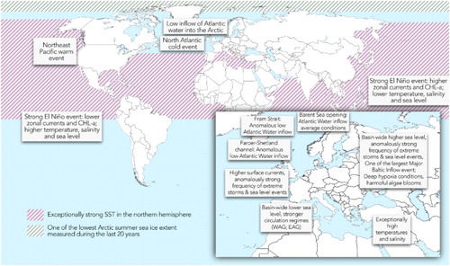
As discussed in more detail in the introduction, this report is only a first – but important – step towards a more comprehensive and systematic reporting of the state of the marine environment. Firstly, the report greatly improved the scientific exploitation of CMEMS comprehensive marine environmental data products. Exchanges between CMEMS experts and the research community were strengthened and new collaborations and links between individual European researchers, institutions, programs and projects have been established. Secondly, this activity will pave the way to strengthen the links between other Copernicus services and, in particular, the Copernicus Climate Change Service. Thirdly, a more concrete dialogue can be opened with the user community in order to improve the response to their needs for future ocean state and change reporting. Finally, this first CMEMS OSR builds the fundamental basis for CMEMS Ocean Monitoring Indicators aiming at a regular monitoring of the ocean state, variability and change at global and European scales.

Acknowledgement

The Ocean State Report (OSR) was prepared as part of the Copernicus Marine Environment Monitoring Service (CMEMS) activities. CMEMS is implemented by Mercator Ocean through a Delegation Agreement with the European Union. All teams that contribute to CMEMS are acknowledged for their support to this CMEMS OSR.

Disclosure statement

No potential conflict of interest was reported by the authors.

Notes

1 Four TACs (In-situ, sea level, Ocean Colour and Ocean& Sea Ice) and six MFCs (Global, Arctic, North-West Shelf, IBI area, Mediterranean Sea and Black Sea).

2 NCEO-CCI EXP1.2 product, http://gws-access.ceda.ac.uk/public2/nceo_uor/sst/L3S/EXP1.2/.

3 SST_MED_SST_L4_REP_OBSERVATIONS_010_021 (PUM: http://marine.copernicus.eu/documents/PUM/CMEMS-OSI-PUM-010-021-022.pdf; QUID: http://marine.copernicus.eu/documents/QUID/CMEMS-OSI-QUID-010-021-022.pdf) and SST_BS_SST_L4_REP_OBSERVATIONS_010_022 (PUM: http://marine.copernicus.eu/documents/PUM/CMEMS-OSI-PUM-010-021-022.pdf; QUID: http://marine.copernicus.eu/documents/QUID/CMEMS-OSI-QUID-010-021-022.pdf).

4 SST_MED_SST_L4_NRT_OBSERVATIONS_010_004 (PUM: http://marine.copernicus.eu/documents/PUM/CMEMS-OSI-PUM-010-004-006-012-013.pdf; QUID: http://marine.copernicus.eu/documents/QUID/CMEMS-OSI-QUID-010-004-006-012-013.pdf) and SST_BS_SST_L4_NRT_OBSERVATIONS_010_006 (PUM: http://marine.copernicus.eu/documents/PUM/CMEMS-OSI-PUM-010-004-006-012-013.pdf; QUID: http://marine.copernicus.eu/documents/QUID/CMEMS-OSI-QUID-010-004-006-012-013.pdf).

5 SST_GLO_SST_L4_NRT_OBSERVATIONS_010_001 (PUM: http://marine.copernicus.eu/documents/PUM/CMEMS-OSI-PUM-010-001.pdf; QUID: http://marine.copernicus.eu/documents/QUID/CMEMS-OSI-QUID-010-001.pdf).

6 SST_GLO_SST_L4_REP_OBSERVATIONS_010_011 (PUM: http://marine.copernicus.eu/documents/QUID/CMEMS-OSI-QUID-010-011.pdf; QUID: http://marine.copernicus.eu/documents/PUM/CMEMS-OSI-PUM-010-011.pdf).

7 GLOBAL_REP_PHYS_001_013 (PUM: http://marine.copernicus.eu/documents/PUM/CMEMS-GLO-PUM-001-013.pdf; QUID: http://marine.copernicus.eu/documents/QUID/CMEMS-GLO-QUID-001-013.pdf).

8 MEDSEA_REANALYSIS_PHYS_006_004 and analysis (PUM: http://marine.copernicus.eu/documents/PUM/CMEMS-MED-PUM-006-004.pdf; QUID: http://marine.copernicus.eu/documents/QUID/CMEMS-MED-QUID-006-004.pdf).

9 MEDSEA_ANALYSIS_FORECAST_PHYS_006_001 (PUM: http://marine.copernicus.eu/documents/PUM/CMEMS-MED-PUM-006-001.pdf: QUID: http://marine.copernicus.eu/documents/QUID/CMEMS-MED-QUID-006-001.pdf).

10 INSITU_MED_TS_REP_OBSERVATIONS_013_041 (PUM: http://marine.copernicus.eu/documents/PUM/CMEMS-INS-PUM-013.pdf; QUID: http://marine.copernicus.eu/documents/QUID/CMEMS-INS-QUID-013-041.pdf).

11 OCEANCOLOUR_GLO_CHL_L3_REP_OBSERVATIONS_009_065 (PUM: http://marine.copernicus.eu/documents/PUM/CMEMS-OC-PUM-009-ALL.pdf; QUID: http://marine.copernicus.eu/documents/QUID/CMEMS-OC-QUID-009-064-065-093.pdf).

12 INSITU_GLO_UV_L2_REP_OBSERVATIONS_013_044 (PUM: http://marine.copernicus.eu/documents/PUM/CMEMS-INS-PUM-013-044.pdf; QUID: http://marine.copernicus.eu/documents/QUID/CMEMS-INS-QUID-013-044.pdf).

13 GLOBAL_REANALYSIS_PHYS_001_025 (PUM: http://marine.copernicus.eu/documents/PUM/CMEMS-GLO-PUM-001-025-011-017.pdf; QUID: http://marine.copernicus.eu/documents/QUID/CMEMS-GLO-QUID-001-025-011-017.pdf.

14 ARCTIC_REANALYSIS_PHYS_002_003 (PUM: http://marine.copernicus.eu/documents/PUM/CMEMS-ARC-PUM-002-ALL.pdf; QUID: http://marine.copernicus.eu/documents/QUID/CMEMS-ARC-QUID-002-003.pdf).

15 ARCTIC_ANALYSIS_FORECAST_PHYS_002_001_a (PUM: http://marine.copernicus.eu/documents/PUM/CMEMS-ARC-PUM-002-ALL.pdf; QUID: http://marine.copernicus.eu/documents/QUID/CMEMS-ARC-QUID-002-001a.pdf).

16 SEAICE_GLO_SEAICE_L4_REP_OBSERVATIONS_011_009 (PUM: http://marine.copernicus.eu/documents/PUM/CMEMS-OSI-PUM-011-009.pdf; QUID: http://marine.copernicus.eu/documents/QUID/CMEMS-OSI-QUID-011-001to007-009to012.pdf) SEAICE_ARC_SEAICE_L3_REP_OBSERVATIONS_011_010.

17 For the period 1993-2014, the CMEMS product NSITU_GLO_TS_REP_OBSERVATIONS_013_001_b (PUM: http://marine.copernicus.eu/documents/PUM/CMEMS-INS-PUM-013-001-b.pdf; QUID: http://marine.copernicus.eu/documents/QUID/CMEMS-INS-QUID-013-001b.pdf). has been used and the time series is extended using the CMEMS near-real-time product INSITU_GLO_NRT_OBSERVATIONS_013_030 (PUM: http://marine.copernicus.eu/documents/PUM/CMEMS-INS-PUM-013.pdf; QUID: http://marine.copernicus.eu/documents/QUID/CMEMS-INS-QUID-013-030-036.pdf).

18 NORTHWESTSHELF_ANALYSIS_FORECAST_PHYS_004_001_b (PUM: http://marine.copernicus.eu/documents/PUM/CMEMS-NWS-PUM-004-001.pdf; QUID: http://marine.copernicus.eu/documents/QUID/CMEMS-NWS-QUID-004-001-002.pdf).

19 NORTHWESTSHELF_REANALYSIS_PHYS_004_009 (PUM: http://marine.copernicus.eu/documents/PUM/CMEMS-NWS-PUM-004-009-011.pdf; QUID: http://marine.copernicus.eu/documents/QUID/CMEMS-NWS-QUID-004-009-011.pdf).

20 BALTICSEA_ANALYSIS_FORECAST_PHYS_003_006 (PUM: http://marine.copernicus.eu/documents/PUM/CMEMS-BAL-PUM-003-006.pdf; QUID: http://marine.copernicus.eu/documents/QUID/CMEMS-BAL-QUID-003-006.pdf).

21 IBI_ANALYSIS_FORECAST_PHYS_005_001_b (PUM: http://marine.copernicus.eu/documents/PUM/CMEMS-IBI-PUM-005-001.pdf; QUID: http://marine.copernicus.eu/documents/QUID/CMEMS-IBI-QUID-005-001.pdf).

22 IBI_REANALYSIS_PHYS_005_002 (PUM: http://marine.copernicus.eu/documents/PUM/CMEMS-IBI-PUM-005-002.pdf; QUID: http://marine.copernicus.eu/documents/QUID/CMEMS-IBI-QUID-005-002.pdf)

23 INSITU_BAL_NRT_OBSERVATIONS_013_032 (PUM: http://marine.copernicus.eu/documents/PUM/CMEMS-INS-PUM-013.pdf; QUID: http://marine.copernicus.eu/documents/QUID/CMEMS-INS-QUID-013-030-036.pdf).

24 INSITU_IBI_TS_REP_OBSERVATIONS_013_040 (PUM: http://marine.copernicus.eu/documents/PUM/CMEMS-INS-PUM-013.pdf; QUID: http://marine.copernicus.eu/documents/QUID/CMEMS-INS-QUID-013-040.pdf).

25 INSITU_NWS_TS_REP_OBSERVATIONS_013_043 (PUM: http://marine.copernicus.eu/documents/PUM/CMEMS-INS-PUM-013.pdf; QUID: http://marine.copernicus.eu/documents/QUID/CMEMS-INS-QUID-013-043.pdf).

26 INSITU_BAL_TS_REP_OBSERVATIONS_013_038 (PUM: http://marine.copernicus.eu/documents/PUM/CMEMS-INS-PUM-013.pdf; http://marine.copernicus.eu/documents/QUID/CMEMS-INS-QUID-013-038.pdf).

References

- Introductions
- Blunden J. Arndt DS. editors. 2016. State of the climate in 2015. Bull Amer Meteorol Soc. 97:S1–S275. doi: 10.1175/2016BAMSStateoftheClimate.1
- Bojinski S, Verstraete M, Peterson TC, Richter C, Simmons A, Zemp M. 2014. The concept of essential climate variables in support of climate research, applications, and policy. Bull Amer Meteorol Soc. 95:1431–1443. doi: 10.1175/BAMS-D-13-00047.1
- CMEMS. 2014. Technical annex to the delegation agreement with Mercator Ocean for the implementation of the Copernicus Marine Environment Monitoring Service (CMEMS). Available from: http://www.copernicus.eu/sites/default/files/library/CMEM_TechnicalAnnex_PUBLIC.docx.pdf.
- CMEMS. 2016. High level service evolution strategy, a document prepared by Mercator Ocean with the support of the CMEMS STAC.
- GCOS. 2010. Implementation plan for the global observing system for climate in support of the UNFCCC (2010 update). GCOS Rep. 138:186. Available from: www.wmo.int/pages/prog/gcos/Publications/gcos-138.pdf.
- Hansen J, Sato M, Kharecha P, von Schuckmann K. 2011. Earth’s energy imbalance and implications. Atmos Chem Phys. 11:13421–13449. doi:10.5194/acp-11-13421-2011.
- Hernandez F, Blockley E, Brassington GB, Davidson F, Divakaran P, Drévillon M, Ishizaki S, Garcia-Sotillo M, Hogan PJ, Lagemaa P, et al. 2015. Recent progress in performance evaluations and near real-time assessment of operational ocean products. J Oper Oceanogr. 8:s221–s238. doi:10.1080/1755876X.2015.1050282.
- IFSOO. 2012. A framework for ocean observing. By the task team for an integrated framework for sustained ocean observing, UNESCO 2012, IOC/INF-1284. doi:10.5270/OceanObs09-FOO.
- IPCC. 2013. Paper presented at the 5th assessment report, the physical science basis. Contribution of Working Group I to the Fifth Assessment Report of the Intergouvernmental Panel on Climate Change.
- IPCC. 2014. Summary for policymakers. In: Field CB, Barros VR, Dokken DJ, Mach KJ, Mastrandrea MD, Bilir TE, Chatterjee M, Ebi KL, Estrada YO, Genova RC, et al., editors. Climate change 2014: impacts, adaptation, and vulnerability. Part A: global and sectoral aspects. Contribution of Working Group II to the Fifth Assessment Report of the Intergovernmental Panel on Climate Change. Cambridge (UK): Cambridge University Press; p. 1–32.
- Le Quéré C, Moriarty R, Andrew RM, Canadell JG, Sitch S, Korsbakken JI, Friedlingstein P, Peters GP, Andres RJ, Boden TA, et al. 2015. Global carbon budget 2015. Earth Syst Sci Data. 7:349–396. doi:10.5194/essd-7-349-2015.
- Levitus S, Antonov J, Boyer T. 2005. Warming of the world ocean, 1955–2003. Geophys Res Lett. 32:L02604. doi:10.1029/2004GL021592.
- CHAPTER 1
- Section 1.1
- Buongiorno Nardelli B, Colella S, Santoleri R, Guarracino M, Kholod A. 2010. A re-analysis of Black Sea surface temperature. J Marine Syst. 79:50–64. doi:10.1016/j.marsys.2009.07.001.
- Chelton DB, Wentz FJ. 2005. Global microwave satellite observations of sea surface temperature for numerical weather prediction and climate research. Bull Amer Meteor Soc. 86:1097–1115. doi: 10.1175/BAMS-86-8-1097
- Feudale L, Shukla J. 2007. Role of Mediterranean SST in enhancing the European heat wave of summer 2003. Geophys Res Lett. 34: L03811. doi:10.1029/2006GL027991.
- Jung T, Ferranti L, Tompkins AM. 2006. Response to the Summer of 2003 Mediterranean SST Anomalies over Europe and Africa. J Clim. 19:5439–5454. doi:10.1175/JCLI3916.1.
- Jungclaus, JH, Haak H, Esch M, Roeckner E, and Marotzke J. 2006. Will Greenland melting halt the thermohaline circulation? Geophys. Res. Lett., 33, L17708, doi:10.1029/2006GL026815.
- Kendall MG. 1975. Multivariate analysis. London: Charles Griffin & Co; p. 210, 43.
- Mann HB. 1945. Nonparametric tests against trend. Econometrica. 13:245–259. p. 42. doi: 10.2307/1907187
- Marsouin A, Le Borgne P, Legendre G, Péré S, Roquet H. 2016. Six years of OSI-SAF METOP-A AVHRR sea surface temperature. Remote Sens Environ. 159:288–306. doi:10.1016/j.rse.2014.12.018.
- Marullo S, Santoleri R, Ciani D, Le Borgne P, Péré S, Pinardi N, Tonani M, Nardone G. 2014. Combining model and geostationary satellite data to reconstruct hourly SST field over the Mediterranean Sea. Remote Sens Environ. 146:11–23. doi:10.1016/j.rse.2013.11.001.
- Merchant CJ, Embury O, Roberts-Jones J, Fiedler E, Bulgin CE, Corlett GK, Good S, McLaren A, Rayner N, Morak-Bozzo S, Donlon C. 2014. Sea surface temperature datasets for climate applications from Phase 1 of the European Space Agency Climate Change Initiative (SST CCI). Geoscience Data Journal. 1:179–191. doi:10.1002/gdj3.20.
- Newman M, Compo GP, Alexander MA. 2003. ENSO-forced variability of the pacific decadal oscillation. J Clim. 16:3853–3857. doi:10.1175/1520-0442(2003)016<3853:EVOTPD>2.0.CO;2.
- Pisano A, Buongiorno Nardellia B, Tronconia C, Santoleria R. 2016. The new Mediterranean optimally interpolated pathfinder AVHRR SST Dataset (1982–2012). Remote Sensing of Environment. 176. 107–116. doi=10.1016/j.rse.2016.01.019. doi: 10.1016/j.rse.2016.01.019
- Roberts-Jones J, Fiedler EK, Martin M. 2011. Description and assessment of the OSTIA reanalysis. UK: Met Office, Forecasting Research Technical Report 561. Available from: http://www.metoffice.gov.uk/media/pdf/h/e/FRTR561.pdf.
- Sen PK. 1968. Estimates of the regression coefficient based on Kendall’s tau. J Am Statist Assoc. 63:1379–1389. doi: 10.1080/01621459.1968.10480934
- Shapiro GI, Aleynik DL, Mee LD. 2010. Long term trends in the sea surface temperature of the Black Sea. Ocean Sci. 6:491–501. doi:10.5194/os-6-491-2010.
- Stocker TF, Qin D, Plattner G-K, Alexander LV, Allen SK, Bindoff NL, Bréon F-M, Church JA, Cubasch U, Emori S, et al. 2013. Technical summary. In: Stocker TF, Qin D, Plattner G-K, Tignor M, Allen SK, Boschung J, Nauels A, Xia Y, Bex V, Midgley PM, editors. Climate Change 2013: the physical science basis. Contribution of Working Group I to the Fifth Assessment Report of the Intergovernmental Panel on Climate Change. Cambridge (UK): Cambridge University Press; p. 33–115. doi:10.1017/CBO9781107415324.005.
- Section 1.2:
- Bond NA, Cronin MF, Freeland H. 2015. The blob: an extreme warm anomaly in the Northeast Pacific [in “State of the climate in 2014”]. Bull Am Meteorol Soc. 96:S62–S63.
- Forget G, Wunsch C. 2007. Estimated global hydrographic variability. J Phys Oceanogr. 37:1997–2008. doi:10.1175/JPO3072.1.
- Grist JP, Josey SA, Jacobs ZL, Marsh R, Sinha B, Van Sebille E. 2016. Extreme air–sea interaction over the North Atlantic subpolar gyre during the winter of 2013–2014 and its sub surface legacy. Clim Dynam. doi:10.1007/s00382-015-2819-3.
- Guinehut S, Dhomps A-L, Larnicol G, Le Traon P-Y. 2012. High resolution 3-D temperature and salinity fields derived from in situ and satellite observations. Ocean Sci. 8:845–857. doi:10.5194/os-8-845-2012.
- Menna M, Poulain P-M, Zodiatis G, Gertman I. 2012. On the surface circulation of the Levantine sub-basin derived from Lagrangian drifters and satellite altimetry data. Deep Sea Res Part 1 Oceanogr Res Pap. 65:46–58. doi: 10.1016/j.dsr.2012.02.008
- Riser SC, Freeland HJ, Roemmich D, Wijffels S, Triosi A, Belbéoch M, Gilbert D, Xu J, Pouliquen S, Thresher A, et al. 2016. Fifteen years of ocean observations with the global Argo array. Nat Clim Chang. 6:145–153. doi:10.1038/nclimate2872.
- Roemmich D, Church J, Gilson J, Monselesan D, Sutton P, Wijffels S. 2015. Unabated planetary warming and its ocean structure since 2006. Nat Clim Chang. 5:240–245. doi:10.1038/NCLIMATE2513.
- Roemmich D, Gilson J. 2011. The global ocean imprint of ENSO. Geophys Res Lett. 38:L13606. doi:10.1029/2011GL047992.
- Talley LD. 2008. Freshwater transport estimates and the global overturning circulation: shallow, deep and throughflow components. Prog Oceanogr. 78:257–303. doi:10.1016/j.pocean.2008.05.001.
- Wijffels S, Roemmich D, Monselesan D, Church J, Gilson J. 2016. Ocean temperatures chronicle the ongoing warming of Earth. Nat Clim Change. 6:116–118. doi:10.1038/nclimate2924.
- Section 1.3:
- Boyer TP, Levitus S, Antonov JI, Locarnini RA, Garcia HE. 2005. Linear trends in salinity for the world ocean, 1955–1998. Geophys Res Lett. 32:L01604. doi:10.1029/2004GL021791.
- Cravatte S, Delcroix T, Zhang D, McPhaden M, Leloup J. 2009. Observed freshening and warming of the western Pacific Warm Pool. Clim Dyn. 33:565–589. doi:10.1007/s00382-009-0526-7.
- Curry R, Dickson B, Yashayaev I. 2003. A change in the freshwater balance of the Atlantic Ocean over the past four decades. Nature. 426:826–829. doi:10.1038nature02206.
- Durack PJ. 2015. Ocean salinity and the global water cycle. Oceanography. 28:20–31. doi:10.5670/oceanog.2015.03.
- Durack PJ, Lee T, Vinogradova NT, Stammer D. 2016. Keeping the lights on for global ocean salinity observation. Nat Clim Chang. 6:228–231. doi:10.1038/nclimate2946.
- Durack PJ, Wijffels SE. 2010. Fifty-year trends in global ocean salinities and their relationship to broad-scale warming. J Clim. 23:4342–4362. doi:10.1175/2010JCLI3377.1.
- Durack PJ, Wijffels SE, Gleckler PJ. 2014. Long-term sea-level change revisited: the role of salinity. Environ Res Lett. 9:114017. doi:10.1088/1748-9326/9/11/114017.
- Fasullo JT, Boening C, Landerer FW, Nerem RS. 2013. Australia’s unique influence on global sea-level in 2010–2011. Geophys Res Lett. 40:4368–4373. doi:10.1002/grl.50834.
- Good SA, Martin MJ, Rayner NA. 2014. EN4: quality controlled ocean temperature and salinity profiles and monthly objective analyses with uncertainty estimates. J Geophys Res. 118:6704–6716. doi:10.1002/2013JC009067.
- Hosoda S, Suga T, Shikama N, Mizuno K. 2009. Global surface layer salinity change detected by Argo and its implication for hydrological cycle intensification. J Oceanogr. 65:579–586. doi:10.1007/s10872-009-0049-1.
- Josey SA, Gulev S, Yu L. 2013. Exchanges through the ocean surface. In: Siedler G, Griffies SM, Gould J, Church JA, editors. Ocean circulation and climate: a 21st century perspective. International Geophysics, Vol. 103. Oxford (UK): Academic Press, Elsevier; p. 115–140. doi:10.1016/B978-0-12-391851-2.00005-2.
- Menna M, Poulain P-M. 2010. Mediterranean intermediate circulation estimated from Argo data in 2003–2010. Ocean Sci. 6:331–343. doi: 10.5194/os-6-331-2010
- Notarstefano G, Poulain P-M. 2009. Thermohaline variability in the Mediterranean and Black Seas as observed by Argo floats in 2000–2009. Technical Report OGS 2009/121 OGA 26 SIRE, 1–77.
- Pinardi N, Zavatarelli M, Adani M, Coppini G, Fratianni C, Oddo P, Simoncelli S, Tonani M, Lyubartsev V, Dobricic S, Bonaduce A. 2015. Mediterranean Sea large-scale low-frequency ocean variability and water mass formation rates from 1987 to 2007: a retrospective analysis. Prog Oceanogr. 132:318–332. doi:10.1016/j.pocean.2013.11.003.
- Tchilibou M, Delcroix T, Alory G, Arnault S, Reverdin G. 2015. Variations of the tropical Atlantic and Pacific SSS minimum zones and their relations to the ITCZ and SPCZ rain bands (1979–2009). J Geophys Res Oceans. 120:5090–5100. doi:10.1002/2015JC010836.
- Terray L, Corre L, Cravatte S, Delcroix T, Reverdin G, Ribes A. 2012. Near-surface salinity as nature’s rain gauge to detect human influence on the tropical water cycle. J Clim. 25:958–977. doi:10.1175/JCLI-D-10-05025.1.
- Trenberth KE, Smith L, Qian T, Dai A, Fasullo J. 2007. Estimates of the global water budget and its annual cycle using observational and model data. J Hydrometeorolog. 8:758–769. doi:10.1175/JHM600.1.
- von Schuckmann K, Gaillard F, Le Traon PY. 2009. Global hydrographic variability patterns during 2003–2008. J Geophys Res. 114:C09007. doi:10.1029/2008JC005237.
- Wüst G. 1936. Oberflächensalzgehalt, Verdunstung und Niederschlag auf dem Weltmeere. Länderkundliche Forschung, Festschrift Norbert Krebs. 347–359.
- Yu L, Adler RF, Huffman GJ, Jin X, Kato S, Loeb NG, Stackhouse PW, Weller RA, Wilber AC. 2015. Ocean surface heat, freshwater, and momentum fluxes [in “State of the climate in 2015”]. Bull Am Meteorol Soc. 97:S74–S77.
- Zu Z, Poulain P-M, Notarstefano G. 2014. Changes in hydrological properties of the Mediterranean Sea over the last 40 years with focus on the Levantine Intermediate Water and the Atlantic Water. Report of the istituto nazionale di Oceanografia e di Geofisica Sperimentale (Italy). 2014/74 Sez. OCE 26 MAOS. p. 37.
- Section 1.4:
- Ablain M, Cazenave A, Larnicol G, Balmaseda M, Cipollini P, Faugère Y, Fernandes MJ, Henry O, Johannessen JA, Knudsen P, et al. 2015. Improved sea level record over the satellite altimetry era (1993–2010) from the Climate Change Initiative project. Ocean Sci. 11:67–82. doi:10.5194/os-11-67-2015.
- Ablain M, Legeais J-F, Prandi P, Marcos M, Fenoglio-Marc L, Dieng HB, Benveniste J, Cazenave A. 2016. Altimetry-based sea-level at global and regional scales. Surv Geophys. doi:10.1007/s10712-016-9389-8.
- Boening C, Willis JK, Landerer FW, Nerem RS, Fasullo J. 2012. The 2011 La Niña: so strong, the oceans fell. Geophys Res Lett. 39:L19602. doi:10.1029/2012GL053055.
- Bonaduce A, Pinardi N, Oddo P, Spada G, Larnicol G. 2016. Sea-level variability in the Mediterranean sea from altimetry and tide gauges. Clim Dyn. February: 1–16. doi:10.1007/s00382-016-3001-2.
- Capotondi A, Wittenberg AT, Newman M, Di Lorenzo E, Yu J-Y, Braconnot P, Cole J, Dewitte B, Giese B, Guilyardi E, et al. 2015. Understanding enso diversity. Bull Am Meteorol Soc. 96:921–938. doi:10.1175/BAMS-D-13-00117.I.
- Cazenave A, Dieng H-B, Meyssignac B, von Schuckmann K, Decharme B, Berthier E. 2014. The rate of sea-level rise. Nat Geosci. doi:10.1038/NCLIMATE2159.
- Cazenave A, Remy F. 2011. Sea level and climate: measurements and causes of changes. WIREs Clim Change. 2:647–662. doi:10.1002/wcc.139.
- Demirov E, Pinardi N. 2002. Simulation of the Mediterranean sea circulation from 1979 to 1993: Part I. The interannual variability. J Marine Syst. 33–34:23–50. doi:10.1016/S0924-7963(02)00051-9.
- Dieng HB, Henry O, von Schuckmann K, Meyssignac B, Cazenave A, Palanisamy H, Lemoine J-M. 2014. Effect of La Nina on the global mean sea-level and north Pacific ocean mass over 2005–2011. J Geod Sci. 4:19–27. doi:10.2478/jogs-2014-0003.
- Dieng HB, Palanisamy H, Cazenave A, Meyssignac B, von Schuckmann K. 2015. The sea-level budget since 2003: inference on the deep ocean heat content. Sur Geophys. 36:209–229. doi:10.1007/s10712-015-9314-6.
- Douglas BC. 1997. Global sea rise: a redetermination. Sur Geophys. 18:279–92. doi:10.1023/A:1006544227856.
- Forget G, Ponte RM. 2015. The partition of regional sea level variability. Prog Oceanogr. 137:173–195. doi: 10.1016/j.pocean.2015.06.002
- Fukumori I, Menemenlis D, Lee T. 2007. A Near-uniform basin-wide sea-level fluctuation of the Mediterranean Sea. J Phys Ocean. 37:338–358. doi: 10.1175/JPO3016.1
- Fukumori I, Wang O. 2013. Origins of heat and freshwater anomalies underlying regional decadal sea-level trends. Geophys Res Lett. 40:563–567. doi: 10.1002/grl.50164
- Han W, Meehl GA, Rajagopalan B, Fasullo JT, Hu A, Lin J, Large WG, Wang J-W, Quan, X-W, Trenary LL, et al. 2010. Patterns of Indian Ocean sea-level change in a warming climate. Nat Geosci. 3:546–550. doi: 10.1038/ngeo901
- Jevrejeva S, Moore JC, Grinsted A, Woodworth PL. 2008. Recent global sea level acceleration started over 200 years ago?. Geophys Res Lett. 35:L08715. doi:10.1029/2008GL033611.
- Legeais J-F, Prandi P, Guinehut S. 2016. Analyses of altimetry errors using Argo and GRACE data. Ocean Sci. 12:647–662. doi:10.5194/os-12-647-2016.
- Levitus S, Antonov JI, Boyer TP, Baranova OK, Garcia HE, Locarnini RA, Mishonov AV, Reagan JR, Seidov D, Yarosh ES, Zweng MM. 2012. World ocean heat content and thermosteric sea-level change (0–2000m), 1955–2010. Geophys Res Lett. 39:L10603. doi:10.1029/2012GL051106.
- Llovel W, Willis JK, Landerer FW, Fukumori I. 2014. Deep-ocean contribution to sea level and energy budget not detectable over the past decade. Nat Clim Change. 4:1031–1035. doi:10.1038/NCLIMATE2387.
- Lombard A, Garric G, Penduff T. 2009. Regional patterns of observed sea level change: insights from a 1/4° global ocean/sea-ice hindcast. Ocean Dynam. 59:433–449. doi: 10.1007/s10236-008-0161-6
- McGregor S, Gupta AS, England MH. 2012. Constraining wind stress products with sea surface height observations and implications for Pacific Ocean sea-level trend attribution. J Clim. 25:8164–8176. doi: 10.1175/JCLI-D-12-00105.1
- Merrifield MA, Merrifield ST, Mitchum GT. 2009. An anomalous recent acceleration of global sea-level rise. J Clim. 22:5772–5781. doi: 10.1175/2009JCLI2985.1
- Merrifield MA, Thompson PR, Lander M. 2012. Multidecadal sea level anomalies and trends in the western tropical Pacific. Geophys Res Lett. 39, L13602. doi:10.1029/2012GL052032.
- Mohrholz V, Naumann MM, Nausch G, Krüger S, Gräwe U. 2015. Fresh oxygen for the Baltic Sea—an exceptional saline inflow after a decade of stagnation. J Mar Syst. 148:152–166. doi: 10.1016/j.jmarsys.2015.03.005
- Nerem RS, Chambers DP, Choe C, Mitchum GT. 2010. Estimating mean sea-level change from the TOPEX and Jason altimeter missions. Mar Geod. 33:435–446. doi: 10.1080/01490419.2010.491031
- Palanisamy H, Cazenave A, Delcroix T, Meyssignac B. 2014. Spatial trend patterns in Pacific Ocean sea-level during the altimetry era: the contribution of thermocline depth change and internal climate variability. Ocean Dynam. doi:10.1007/s10236-014-0805-7.
- Pinardi N, Masetti E. 2000. Variability of the large scale general circulation of the Mediterranean Sea from observations and modelling: a review. Palaeogeogr Palaeocl. 158:153–173. ISSN 0031-0182. doi:10.1016/S0031-0182(00)00048-1.
- Pinardi N, Zavatarelli M, Adani M, Coppini G, Fratianni C, Oddo P, Simoncelli S, Tonani M, Lyubartsev V, Dobricic S, Bonaduce A. 2015. Mediterranean sea large-scale low-frequency ocean variability and water mass formation rates from 1987 to 2007: a retrospective analysis. Prog Oceanogr. 132:318–32. doi:10.1016/j.pocean.2013.11.003.
- Prandi P, Ablain M, Zawadzki L, Meyssignac B. 2016. How reliable are local sea-level trends? In prep.
- Pujol M-I, Faugère Y, Taburet G, Dupuy S, Pelloquin C, Ablain M, Picot N. 2016. DUACS DT 2014: the new multimission altimeter dataset reprocessed over 20 years. Ocean Sci Discuss. in review. doi:10.5194/os-2015-110.
- Rietbroek R, Brunnabend SE, Kusche J, Schröter J, Dahle, C. 2016. Revisiting the contemporary sea-level budget on global and regional scales. Proc Natl A Sci. 113:1504–1509. doi: 10.1073/pnas.1519132113
- von Schuckmann K, Palmer MD, Trenberth KE, Cazenave A, Chambers D, Champollion N, Hansen J, Josey SA, Loeb N, Mathieu P-P, et al. 2016. An imperative to monitor Earth’s energy imbalance. Nat Clim Change. 6:138–144. doi: 10.1038/nclimate2876
- Schiermeir Q. 2015. Hunting the Gozilla El Nino. Nature. 526:490–491. doi:10.1038/526490a.
- Stammer D, Cazenave A, Ponte RM, Tamisiea ME. 2013. Causes for contemporary regional sea-level changes. Annu Rev Mar Sci. 5:21–46. doi:10.1146/annurev-marine-121211-172406.
- Tamisiea M. 2011. Ongoing glacial isostatic contributions to observations of sea level change. Geophy J Int. 186:1036–1044. doi:10.1111/j.1365-246X.2011.05116.
- Woppelmann G, Letetrel C, Santamaria A, Bouin MN, Collilieux X, Altamimi Z, Williams SDP, Miguez BM. 2009. Rates of sea-level change over the past century in a geocentric reference frame. Geophys Res Lett. 36. doi: 10.1029/2009gl038720.
- Wunsch C, Ponte RM, Heimbach P. 2007. Decadal trends in sea-level patterns: 1993–2004. J Clim. 20:5889–5911. doi: 10.1175/2007JCLI1840.1
- Section 1.5:
- Behrenfeld MJ, O’Malley RT, Siegel DA, McClain CR, Sarmiento JL, Feldman GC, Milligan AJ, Falkowski PG, Letelier RM, Boss ES. 2006. Climate-driven trends in contemporary ocean productivity. Nature. 444:752–755. doi:10.1038/nature05317.
- Brewin RJW, Hirata T, Hardman-Mountford NJ, Lavender S, Sathyendranath S, Barlow R. 2012. The influence of the Indian Ocean dipole on interannual variations in phytoplankton size structure as revealed by Earth Observation. Deep Sea Res II. 77-80:117–127. doi:10.1016/j.dsr2.2012.04.009.
- Campbell JW. (1995). The lognormal distribution as a model for bio-optical variability in the sea. J Geophys Res. 100:13237–13254. doi: 10.1029/95JC00458
- Cota GF, Wang J, Comiso JC. 2004. Transformation of global satellite chlorophyll retrievals with a regionally tuned algorithm. Remote Sens Environ. 90:373–377. doi: 10.1016/j.rse.2004.01.005
- Doney SC. 2006. Oceanography: plankton in a warmer world. Nature. 444:695–696. doi: 10.1038/444695a
- GCOS. 2011. Systematic observation requirements from satellite-based data products for climate Technical report, World Meteorological Organisation (WMO), 7 bis, avenue de la Paix, CH-1211 Geneva 2, Switzerland.
- IOCCG. 2014. Phytoplankton functional types from space. In: Sathyendranath S, editor. Reports of the International Ocean-Colour Coordinating Group, No. 15. Dartmouth (Canada): IOCCG. p. 1–154.
- Longhurst A, Sathyendranath S, Platt T, Caverhill C. 1995. An estimate of global primary production in the ocean from satellite radiometer data. J Plankton Res. 17:1245–1271. doi: 10.1093/plankt/17.6.1245
- Nair A, Sathyendranath S, Platt T, Morales J, Stuart V, Forget M-H, Devred E, Bouman H. 2008. Remote sensing of phytoplankton functional types. Remote Sens Environ. 112:3366–3375. doi: 10.1016/j.rse.2008.01.021
- O’Reilly JE, Maritorena S, Siegel D, O’Brien MC. 2000. Ocean color chlorophyll a algorithms for SeaWiFs, OC2, and OC4: Technical report. In: Toole D, Mitchell BG, Kahru M, Chavez FP, Strutton P, Cota G, Hooker SB, McClain CR, Carder KL, Muller-Karger F, et al., editors. SeaWiFS postlaunch calibration and validation analyses, Part 3. SeaWiFS Postlaunch Technical Report Series, Vol. 11. Greenbelt (MD): NASA, Goddard Space Flight Center; p. 9–23.
- Pitarch J, Volpe G, Colella S, Krasemann H, Santoleri R. 2016. Remote sensing of chlorophyll in the Baltic Sea at basin scale from 1997 to 2012 using merged multi-sensor data. Ocean Sci. 12:379–389. doi:10.5194/os-12-379-2016.
- Racault M-F, Le Quéré C, Buitenhuis E, Sathyendranath S, Platt T. 2012. Phytoplankton phenology in the global ocean. Ecol Indic. 14:152–163. doi:10.1016/j.ecolind.2011.07.010.
- Radenac MH, Léger F, Singh A, Delcroix T. 2012. Sea surface chlorophyll signature in the tropical Pacific during eastern and central Pacific ENSO events. J Geophys Res. 117. doi:10.1029/2011JC007841.
- Raitsos DE, Yi X, Platt T, Racault M-F, Brewin RJW, Pradhan Y, Papadopoulos VP, Sathyendranath S, Hoteit I. 2015. Monsoon oscillations regulate fertility of the Red Sea. Geophys Res Lett. 42:855–862. doi:10.1002/2014GL062882.
- Sabine CL, Feely RA, Gruber N, Key RM, Lee K, Bullister JL, Wanninkhof R, Wong C, Wallace DW, Tilbrook B, Millero FJ. 2004. The oceanic sink for anthropogenic CO2. Science. 305:367–371. doi: 10.1126/science.1097403
- Valente A, Sathyendranath S, Brotas V, Groom S, Grant M, Taberner M, Antoine D, Arnone R, Balch WM, Barker K. et al. 2016. A compilation of global bio-optical in-situ data for ocean-colour satellite applications. Earth Syst Sci Data Discuss. in press. doi:10.5194/essd-2015-37.
- Volpe G, Santoleri R, Vellucci V, d’Alcalà MR, Marullo S, d’Ortenzio F. 2007. The colour of the Mediterranean Sea: global versus regional bio-optical algorithms evaluation and implication for satellite chlorophyll estimates. Remote Sens Environ 107:625–638. doi: 10.1016/j.rse.2006.10.017
- Section 1.6:
- Delcroix T, Dewitte B, DuPenhoat Y, Masia F, Picaut J. 2000. Equatorial waves and warm pool displacements during the 1992–1998 El Nino Southern Oscillation events: observation and modeling. J Geophys Res. 105:26045–26062. doi:10.1029/2000JC900113.
- Frankignoul C, de Coëtlogon G, Joyce TM, Dong S. 2001. Gulf Stream variability and ocean–atmosphere interactions. J Phys Oceanogr. 31:3516–3529. doi: 10.1175/1520-0485(2002)031<3516:GSVAOA>2.0.CO;2
- Godfrey JS, Johnson GC, McPhaden MJ, Reverdin G, Wijffels SE. 2001. Chap. 3 The tropical ocean circulation. In Ocean Circulation and Climate. Int Geophys. 77:215–246. doi: 10.1016/S0074-6142(01)80121-2
- Lellouche J-M, Le Galloudec O, Drevillon M, Regnier C, Greiner E, Garric G, Ferry N, Desportes C, Testut C-E, Bricaud C, et al. 2013. Evaluation of global monitoring and forecasting systems at Mercator Ocean. Ocean Sci. 9:57–81. doi:10.5194/os-9-57-2013.
- McPhaden MJ, Busalacchi AJ, Cheney R, Donguy JR, Gage KS, Halpern D, Ming JI, Julian P, Meyers G, Mitchum GT, et al. 1998. The tropical ocean-global atmosphere observing system: A decade of progress. J Geophys Res. 103:14169–14240. doi:10.1029/97JC02906.
- McPhaden MJ. 2015. Playing hide and seek with El Niño. Nat Clim Change. 5:791–795. doi:10.1038/nclimate2775.
- Meinen CS, McPhaden MJ. 2001. Interannual variability in warm water volume transports in the equatorial pacific during 1993–99. J Phys Oceanogr. 31:1324–1345. doi:10.1175/1520-0485(2001).
- Overland J, Rodionov S, Minobe S, Bond N. 2008. North pacific regimes shifts: definitions, issues and recent transitions. Prog Oceanogr. 77:92–102. doi:10.1016/j.pocean.2008.03.016.
- Penduff T, Juza M, Barnier B, Zika J, Dewar WK, Treguier A-M, Molines J-M, Audiffren N. 2011. Sea-level expression of intrinsic and forced ocean variabilities at interannual time scales. J Clim. 24:5652–5670. doi:10.1175/JCLI-D-11-00077.1.
- Reverdin G, Frankignoul C, Kestenare E, McPhaden MJ. 1994. Seasonal variability in the surface currents of the equatorial Pacific. J Geophys Res. 99(C10):20,323–20,344. doi:10.1029/94JC01477.
- Sérazin G, Penduff T, Grégorio S, Barnier B, Molines JM, Terray L. 2015. Intrinsic variability of sea-level from global ocean simulations: spatiotemporal scales. J Clim. 28:4279–4292. doi:10.1175/JCLI-D-14-00554.1.
- Tagushi B, Xie S-P, Schneider N, Nonaka M, Sasaki H, Sasai Y. 2007. Decadal variability of the Kuroshio extension: observations and an Eddy Resolving model Hindcast. J Clim. 20:2357–2377. doi:10.1175/JCLI4142.1.
- Section 1.7:
- Gao Y, Sun J, Li F, He S, Sandven S, Yan Q, Zhang Z, Lohmann K, Keenlyside N, Furevik T, Suo L. 2014. Arctic sea ice and Eurasian climate: a review. Adv Atmos Sci. 32:92–114. doi:10.1007/s00376-014-0009-6.
- Giles KA, Laxon SW, Ridout AL, Wingham DJ, Bacon S. 2012. Western Arctic Ocean freshwater storage increased by wind-driven spin-up of the Beaufort Gyre. Nat Geosci. 5:194–197. doi:10.1038/ngeo1379.
- Kwok R, Rothrock DA. 2009. Decline in Arctic sea ice thickness from submarine and ICESat records: 1958–2008. Geophys Res Lett. 36:1–5. doi:10.1029/2009GL039035.
- Laxon SW, Giles KA, Ridout AL, Wingham DJ, Willatt R, Cullen R, Kwok R, Schweiger A, Zhang J, Haas C, et al. 2013. CryoSat-2 estimates of Arctic sea ice thickness and volume. Geophys Res Lett. 40:732–737. doi:10.1002/grl.50193.
- Meier WN, Hovelsrud GK, van Oort BE, Key JR, Kovacs KM, Michel C, Haas C, Granskog MA, Gerland S, Perovich DK, et al. 2014. Arctic sea ice in transformation: a review of recent observed changes and impacts on biology and human activity. Rev Geophys. 1–33. doi:10.1002/2013RG000431.
- Parkinson CL, Cavalieri DJ. 2012. Antarctic sea ice variability and trends, 1979–2010. Cryosph. 6:871–880. doi:10.5194/tc-6-871-2012.
- Parkinson CL, Comiso JC. 2013. On the 2012 record low Arctic sea ice cover: combined impact of preconditioning and an August storm. Geophys Res Lett. 40:1356–1361. doi:10.1002/grl.50349.
- Rabe B, Karcher M, Kauker F, Schauer U, Toole JM, Krishfield RA, Pisarev S, Kikuchi T, Su J. 2014. Arctic Ocean basin liquid freshwater storage trend 1992–2012. Geophys Res Lett. 41:961–968. doi:10.1002/2013GL058121.
- Stroeve JC, Serreze MC, Fetterer F, Arbetter T, Meier W, Maslanik J, Knowles K. 2005. Tracking the Arctic’s shrinking ice cover: another extreme September minimum in 2004. Geophys Res Lett. 32:1–4. doi:10.1029/2004GL021810.
- Wassmann P, Reigstad M. 2011. Future Arctic Ocean seasonal ice zones and implications for pelagic-benthic coupling. Oceanography. 24:220–231. doi:10.5670/oceanog.2011.74.
- Zygmuntowska M, Rampal P, Ivanova N, Smedsrud LH. 2014. Uncertainties in Arctic sea ice thickness and volume: new estimates and implications for trends. Cryosphere. 8:705–720. doi:10.5194/tc-8-705-2014.
- CHAPTER 2
- Section 2.1:
- Abraham JP, Baringer M, Bindoff NL, Boyer T, Cheng LJ, Church JA, Conroy JL, Domingues CM, Fasullo JT, Gilson J, et al. 2013. A review of global ocean temperature observations: implications for ocean heat content estimates and climate change. Rev Geophys. 51:450–483. doi:10.1002/rog.20022.
- Allan RP, Liu C, Loeb NG, Palmer MD, Roberts M, Smith D, Vidale P-L. 2014. Changes in global net radiative imbalance 1985–2012. Geophys Res Lett. 41: 5588–5597. doi:10.1002/2014GL060962.
- Balmaseda MA, Mogensen K, Weaver AT. 2013. Evaluation of the ECMWF ocean reanalysis system ORAS4. QJR Meteorol Soc. 139:1132–1161. doi:10.1002/qj.2063.
- Balmaseda MA, Trenberth KE, Källén, E. 2013. Distinctive climate signals in reanalysis of global ocean heat content. Geophys Res Lett. 40:1754–1759. doi:10.1002/grl.50382.
- Boyer TT, Domingues CM, Good SA, Johnson GC, Lyman JM, Ishii M, Gouretski V, Willis JK, Antonov J, Wijffels S, et al. 2016. Sensitivity of global upper ocean heat content estimates to mapping methods, XBT bias corrections, and baseline climatologies. J Clim. 29:4817–4842. doi:10.1175/JCLI-D-15-0801.1.
- Church JA, White NJ, Konikow LF, Domingues CM, Cogley JG, Rignot E, Gregory JM, van den Broeke MR, Monaghan AJ, Velicogna I. 2011. Revisiting the earth’s sealevel and energy budgets from 1961 to 2008. Geophys Res Lett. 38:L18601. doi:10.1029/2011GL048794. And Correction: Church JA, White NJ, Konikow LF, Domingues CM, Cogley JG, Rignot E, Gregory JM. 2013. Correction to revisiting the earth’s sea-level and energy budgets for 1961 to 2008. Geophysical Research Letters. doi:10.1002/grl.50752.
- L’Ecuyer TS, Beaudoing H, Rodell M, Olson W, Lin B, Kato S, Clayson CA, Wood E, Sheffield J, Adler R, et al. 2015. The Observed State of the Energy Budget in the Early 21st Century. J Clim. 28:8319–8346. doi:10.1175/JCLI-D-14-00556.1.
- Loeb GN, Lyman JM, Johnson GC, Allan RP, Doelling DR, Wong T, Soden BJ, Stephens GL. 2012. Observed changes in top-of-the-atmosphere radiation and upper-ocean heating consistent within uncertainty. Nat Geosci. doi:10.1038/NGEO1375.
- Mayer M, Haimberger L, Balmaseda MA. 2014. On the energy exchange between tropical ocean basins related to ENSO*. J Clim. 27:6393–6403. doi: 10.1175/JCLI-D-14-00123.1
- Palmer MD, McNeall DJ. 2014. Internal variability of Earth’s energy budget simulated by CMIP5 climate models. Env Res Lett. doi:10.1088/1748-9326/9/3/034016.
- Purkey SG, Johnson GC. 2010. Warming of global abyssal and deep southern ocean between the 1990s and 2000s: contributions to global heat and sea level rise budgets. J. Clim. 23:6336–6351. doi:10.1175/2010JCLI3682.1.
- Roemmich D, Church J, Gilson J, Monselesan D, Sutton P, Wijffels S. 2015. Unabated planetary warming and its ocean structure since 2006. Nat Clim Chang. 5:240–245. doi: 10.1038/nclimate2513
- Roemmich D, Gilson J. 2011. The global ocean imprint of ENSO. Geophys Res Lett. 38:L13606. doi:10.1029/2011GL047992 and doi:10.1038/NCLIMATE2513.
- Stephens GL, Li J-L, Wild M, Clayson CA, Loeb N, Kato S, L’Ecuyer T, Stackhouse Jr PW, Lebsock M, Andrews T. 2012. An update on the Earth’s energy balance in light of new surface energy flux estimates. Nat Geosci. 5:691–696. doi: 10.1038/ngeo1580
- Trenberth K, Fasullo J, von Schuckmann K, Cheng L. 2016. Insights into Earth’s energy imbalance from multiple sources. J Clim. 29:7495–7505. doi:10.1175/JCLI-D-16-0339.1.
- Trenberth KE. 2009. An imperative for adapting to climate change: tracking Earth’s global energy. Curr Opin Env Sust. 1:19–27. doi: 10.1016/j.cosust.2009.06.001
- Trenberth KE, Fasullo JT. 2010. Tracking Earth’s energy. Science. 328:316–317. doi: 10.1126/science.1187272
- Trenberth KE, Fasullo JT, Balmaseda MA. 2014. Earth’s energy imbalance. J Clim. 27:3129–3144. doi:10.1175/JCLI-D-13-00294.
- von Schuckmann K, Le Traon PY. 2011. How well can we derive global ocean indicators from Argo data?. Ocean Sci. 7:783–791. doi:10.5194/os-7-783-2011.
- Section 2.2:
- Cunningham SA, Alderson SG, King BA, Brandon MA. 2003. Transport and variability of the Antarctic circumpolar current in Drake passage. J Geophys Res. 108:8084. doi:10.1029/2001JC001147.
- Ganachaud A. 2003. Large-scale mass transports, water mass formation, and diffusivities estimated from world ocean circulation experiment (WOCE) hydrographic data. J Geophys Res. 108:3213. doi:10.1029/2002JC001565.
- Gordon AL, Susanto RD, Ffield A, Huber BA, Pranowo W, Wirasantosa S. 2008. Makassar Strait throughflow, 2004 to 2006. Geophys Res Lett. 35:L24605. doi:10.1029/2008GL036372.
- Lumpkin R, Speer K. 2007. Global ocean meridional overturning. J Phys Oceanogr. 37:2550–2562. doi:10.1175/JPO3130.1.
- McCarthy GD, Smeed DA, Johns WE, Frajka-Williams E, Moat BI, Rayner D, Baringerd MO, Meinen CS, Collins J, Bryden HL. 2015. Measuring the Atlantic meridional overturning circulation at 26°N. Prog Oceanogr. 130:91–111. doi: 10.1016/j.pocean.2014.10.006
- Provost C, Renault A, Barre N, Senn echael N, Garçon V, Sudre J, Huhn O. 2011. Two repeat crossings of Drake passage in austral summer 2006: short-term variations and evidence for considerable ventilation of intermediate and deep waters. Deep Sea Res Pt II. 58:2555–2571. 2555–2572. doi: 10.1016/j.dsr2.2011.06.009
- Stammer D, Ueyoshi K, Köhl A, Large WB, Josey S, Wunsch C. 2004. Estimating air–sea fluxes of heat, freshwater and momentum through global ocean data assimilation. J Geophys Res. 109:C05023. doi:10.1029/2003JC002082.
- Swart S, Speich S, Ansorge IJ, Goni GJ, Gladyshev S, Lutjeharms JR. 2008. Transport and variability of the Antarctic circumpolar current South of Africa. J Geophys Res. 113:C09014–C09016. doi:10.1029/2007JC004223.
- Talley LD, Reid JL, Robbins PE. 2003. Data-based meridional overturning streamfunctions for the global ocean. J Clim. 16:3213–3226. doi: 10.1175/1520-0442(2003)016<3213:DMOSFT>2.0.CO;2
- Valdivieso M, Haines K, Zuo H, Lea D. 2014. Freshwater and heat transports from global ocean synthesis. J Geophys Res Oceans. 119:394–409. doi:10.1002/2013JC009357.
- Vranes K, Gordon AL. 2005. Comparison of Indonesian throughflow transport observations, Makassar Strait to eastern Indian Ocean. Geophys Res Lett. 32:L10606. doi:10.1029/2004GL022158.
- Section 2.3:
- van Aken HM, de Jong FM, Yashayaev I. 2011. Decadal and multi-decadal variability of Labrador Sea Water in the north-western North Atlantic Ocean derived from tracer distributions: heat budget, ventilation, and advection. Deep-Sea Res Pt I. 58:505–523. doi: 10.1016/j.dsr.2011.02.008
- Borenäs KM, Lundberg PA. 2004. The Faroe-Bank channel deep-water overflow. Deep-Sea Res II. 51:335–350. doi: 10.1016/j.dsr2.2003.05.002
- Brunnabend SE, Schröter J, Rietbroek R, Kusche J. 2015. Regional sea-level change in response to ice mass loss in Greenland, the West Antarctic and Alaska. J Geophys Res Oceans. 120:7316–7328. doi: 10.1002/2015JC011244
- Clarke RA, Swift JH, Reid JL, Koltermann KP. 1990. The formation of Greenland sea deep-water – double diffusion or deep convection. Deep-Sea Res Pt A. 37:1385–1424. doi: 10.1016/0198-0149(90)90135-I
- Duchez A, Frajka-Williams E, Josey S, Evans D, Grist J, Marsh R, McCarthy G, Sinha B, Berry D, Hirschi J. 2016. Drivers of exceptionally cold North Atlantic Ocean temperatures and their link to the 2015 European heat wave. Environ Res Lett. 11:074004. doi:10.1088/1748-9326/11/7/074004.
- Fichefet T, Poncin C, Goosse H, Huybrechts P, Janssens I, Le Treut H. 2003. Implications of changes in freshwater flux from the Greenland ice sheet for the climate of the 21st century. Geophys Res Lett. 30. doi:10.1029/2003GL017826.
- Gladyshev SV, Gladyshev VS, Gulev SK, Sokov AV. 2016. Anomalously deep converction in the Irminger Sea during the winter of 2014–2015. Dok Earth Sci. 469:766–770. doi: 10.1134/S1028334X16070229
- Häkkinen S, Rhines PB, Worthen DL. 2015. Heat content variability in the North Atlantic Ocean in ocean reanalyses. Geophys Res Lett. 42:2901–2909. doi:10.1002/2015GL063299.
- Hansen B, Østerhus S. 2000. North Atlantic – Nordic Seas exchanges. Progess in Oceanogr. 45:109–208. doi: 10.1016/S0079-6611(99)00052-X
- Hermanson L, Eade R, Robinson NH, Dunstone NJ, Andrews MB, Knight JR, Scaife AA, Smith DM. 2014. Forecast cooling of the Atlantic subpolar gyre and associated impacts. Geophys Res Lett. 41:5167–5174. doi:10.1002/2014GL060420.
- Hu AX, Meehl GA, Han WQ, Yin JJ. 2011. Effect of the potential melting of the Greenland Ice Sheet on the Meridional Overturning Circulation and global climate in the future. Deep Sea Res II. 58:1914–1926. doi: 10.1016/j.dsr2.2010.10.069
- Jackson LC, Kahana R, Graham T, Ringer MA, Woollings T, Mecking JV, Wood RA. 2015. Global and European climate impacts of a slowdown of the AMOC in a high resolution GCM. Clim Dynam. 45:3299–3316. doi:10.1007/s00382-015-2540-2.
- Jackson LC, Peterson AK, Roberts CD, Wood RA. 2016. Recent slowing of Atlantic overturning circulation as a recovery from earlier strengthening. Nat Geosci. 1752–0894. doi:10.1038/ngeo2715.
- Jochumsen K, Quadfasel D, Valdimarsson H, Jónsson S. 2012. Variability of the Denmark Strait overflow: moored time series from 1996–2011, J Geophys Res. 117:C12003. doi: 10.1029/2012JC008244
- de Jong FM, van Aken HM, Våge K, Pickart RS. 2012. Convective mixing in the Irminger Sea: 2002–2010. Deep Sea Res Pt I. 63:36–51. doi: 10.1016/j.dsr.2012.01.003
- Josey SA, Grist J, Kieke D, Yashayaev I, Yu L. 2015. Extraordinary ocean cooling and new dense water formation in the North Atlantic (Sidebar 3.2), in: the state of the climate in 2014. Bull Amer Meteor Soc. 96:66–67. doi: 10.1175/BAMS-D-15-00129.1
- Jungclaus JH, Haak H, Esch M, Roeckner E, and Marotzke J. 2006. Will Greenland melting halt the thermohaline circulation? Geophys Res Lett. 33:L17708. doi: 10.1029/2006GL026815
- Karspeck AR, Stammer D, Köhl A, Danabasoglu G, Balmaseda M, Smith DM, Fujii Y, Zhang S, Giese B, Tsujino H, Rosati A. 2015. Comparison of the Atlantic meridional overturning circulation between 1960 and 2007 in six ocean reanalysis products. Clim Dyn. doi:10.1007/s00382-015-2787-7.
- Martin S, Cavalieri DJ. 1989. Contributions of the Siberian shelf polynyas to the Arctic Ocean Intermediate and Deep Water. J Geophys Res. 94:12725–12738. doi: 10.1029/JC094iC09p12725
- McCarthy GD, Haigh ID, Hirschi JJ-M, Grist JP, Smeed DA. 2015. Ocean impact on decadal Atlantic climate variability revealed by sea-level observations. Nature. 521:508–510. doi:10.1038/nature14491.
- Midttun L. 1985. Formation of dense bottom water in the Barents Sea. Deep-Sea Res Pt A. 32:1233–1241. doi: 10.1016/0198-0149(85)90006-8
- Rahmstorf S, Box J, Feulner G, Mann M, Robinson A, Rutherford S, Schaffernicht E. 2015. Exceptional twentieth-century slowdown in Atlantic Ocean overturning circulation. Nat Clim Change. 5/475-480. ISSN 1758-678X. doi:10.1038/nclimate2554.
- Ridley JK, Huybrechts P, Gregory JM, Lowe JA. 2005. Elimination of the Greenland ice sheet in a high CO2 climate. J Clim. 18:3409–3427. doi: 10.1175/JCLI3482.1
- Robson J, Sutton R, Lohmann K, Smith D, Palmer MD. 2012. Causes of the rapid warming of the North Atlantic Ocean in the Mid-1990s. J Clim. 25:4116–4134. doi:10.1175/JCLI-D-11-00443.1.
- Robson J, Hodson D, Hawkins E, Sutton R. 2014. Atlantic overturning in decline? Nat Geosci 7:2–3. ISSN 1752-0894. doi:10.1038/ngeo2050.
- Skogseth R, Smedsrud LH, Nilsen F, Fer I. 2008. Observations of hydrography and downflow of brine-enriched shelf water in the Storfjorden polynya, Svalbard. J Geophys Res. 113:C08049. doi:10.1029/2007JC004452.
- Smeed D, McCarthy G, Rayner D, Moat BI, Johns WE, Baringer MO, Meinen CS. 2016. Atlantic meridional overturning circulation observed by the RAPID-MOCHA-WBTS (RAPID-Meridional overturning circulation and heatflux array-western boundary time series) array at 26N from 2004 to 2015. (UK): British Oceanographic Data Centre - Natural Environment Research Council. doi:10.5285/35784047-9b82-2160-e053-6c86abc0c91b.
- Smeed DA, McCarthy GD, Cunningham SA, Frajka-Williams E, Rayner D, Johns WE, Meinen CS, Baringer MO, Moat BI, Duchez A, Bryden HL. 2014. Observed decline of the Atlantic meridional overturning circulation 2004–2012. Ocean Sci. 10:29–38. doi:10.5194/os-10-29-2014.
- Våge K, Pickart RS, Sarafanov A, Knutsen Ø, Mercier H, Lehrminier P, van Aken HM, Meincke J, Quadfasel D, Bacon S. 2011. The Irminger Gyre: circulation, convection, and interannual variability. Deep Sea Res Pt I. 58:590–614. doi: 10.1016/j.dsr.2011.03.001
- Våge K, Pickart RS, Thierry V, Reverdin G, Lee C, Petrie B, Agnew TA, Wong A, Ribergaard MH. 2009. Surprising return of deep convection to the subpolar North Atlantic Ocean in winter 2007–2008. Nat Geosci. 2:67–72. doi: 10.1038/ngeo382
- Yang Q, Dixon TH, Myers PG, Bonin J, Chambers D, van den Broeke MR. 2016. Recent increases in Arctic freshwater flux affects Labrador Sea convection and Atlantic overturning circulation. Nat Commun. 7:10525. doi:10.1038/ncomms10525.
- Yeager S, Karspeck A, Danabasoglu G, Tribbia J, Teng H. 2012. A decadal prediction case study: late 20th century North Atlantic ocean heat content. J Clim. 25:5173–5189. doi:10.1175/JCLI-D-11-00595.1.
- Section 2.4:
- Arbic BK, Flierl GR. 2004. Baroclinically unstable geostrophic turbulence in the limits of strong and weak bottom Ekman friction: application to midocean eddies. J Phys Oceanogr. 34:2257–2273. doi:10.1175/1520-0485(2004)034<2257:BUGTIT>2.0.CO;2.
- Chelton DB, Schlax MG, Samelson RM. 2011. Global observations of nonlinear mesoscale eddies. Prog Oceanogr. 91:167–216. doi: 10.1016/j.pocean.2011.01.002
- Ducet N, Le Traon PY, Reverdin G. 2000. Global high resolution mapping of ocean circulation from the combination of TOPEX/POSEIDON and ERS-1/2. J Geophys Res. 105:19477–19498. doi: 10.1029/2000JC900063
- Dufour CO, Griffes SM, de Souza GF, Frenger I, Morrison AK, Palter JB, Sarmiento JL, Galbraith ED, Dunne JP, Anderson WG, Slater RD. 2015. Role of mesoscale eddies in cross-frontal transport of heat and biogeochemical tracers in the Southern Ocean. J Phys Oceanogr. 45:3057–3081. doi:10.1175/JPO-D-14-0240.1.
- Duhaut TH, Straub DN. 2006. Wind stress dependence on ocean surface velocity: implications for mechanical energy input to ocean cieculation. J Phys Oceanogr. 36:202–211. doi:10.1175/JPO2842.1.
- Gaube P, McGillicuddy DJ, Chelton DB, Behrenfeld MJ, Strutton PG. 2014. Regional variations in the influence of mesoscale eddies on near-surface chlorophyll. J Geophys Res. 119:8195–8220. doi:10.1002/2014JC010111.
- Gill AE, Green JSA, Simmons AJ. 1974. Energy partition in the large-scale ocean circulation and the production of mid-ocean eddies. Deep Sea Res. 21:499–528.
- Gille ST, Yale MM, Sandwell DT. 2000. Global correlation of Mesoscale Ocean variability with seafloor roughness from satellite altimetry. Geophys Res Lett. 27:1251–1254. doi: 10.1029/1999GL007003
- Godø OR, Samuelsen A, Macaulay GJ, Patel R, Hjøllo SS, Horne J, Kaartvedt S, Johannessen JA. 2012. Mesoscale eddies are oases for higher trophic Marine life. PLoS ONE. 7:e30161. doi:10.1371/journal.pone.0030161.
- Gorsky G, Prieur L, Taupier-Letage I, Stemmann L, Picheral M. 2002. Large particulate matter in the Western Mediterranean I. LPM distribution related to mesoscale hydrodynamics. J Marine Syst. 33:289–311. doi: 10.1016/S0924-7963(02)00063-5
- Heburn GW, La Violette P. 1990. Variations in the structure of the anticyclonic gyres found in the Alboran Sea. J Geophys Res. 95:1599–1613. doi: 10.1029/JC095iC02p01599
- Holland WR. 1978. The role of mesoscale eddies in the general circulation of the ocean – numerical experiments using a wind-driven quasi-geostrophic model. J Phys Oceanogr. 8:363–392. doi: 10.1175/1520-0485(1978)008<0363:TROMEI>2.0.CO;2
- Kang D, Curchitser EN, Rosati A. 2016. Seasonal variability of the gulf stream kinetic energy. J Phys Oceanogr. 46:1189–1207. doi: 10.1175/JPO-D-15-0235.1
- Klein P, Hua BL, Lapeyre G, Capet X, Le Gentil S, Sasaki H. 2008. Upper ocean turbulence from high-resolution 3D simulations. J Phys Oceanogr. 38:1748–1763. doi: 10.1175/2007JPO3773.1
- Klein B, Roether W, Manca BB, Bregant D, Beitzel V, Kovacevic V, Luchette A. 1999. The large deep water transient in the eastern Mediterranean. Deep Sea Res Pt I. 46:371–414. doi: 10.1016/S0967-0637(98)00075-2
- Klein P, Lapeyre G. 2009. The oceanic vertical pump induced by mesoscale and submesoscale turbulence. Annu Rev Mar Sci. 1:351–375. doi: 10.1146/annurev.marine.010908.163704
- Larnicol G, Ayoub N, Le Traon P-Y. 2002. Major changes in Mediterranean Sea level variability from 7 years of TOPEX/Poseidon and ERS-1/2 data. J Marine Syst. 33:63–89 doi: 10.1016/S0924-7963(02)00053-2
- Lee M-M, Marshall DP, Williams RG. 1997. On the Eddy transfer of tracers: advective or diffusive? J Mar Res. 55: 483–505. doi: 10.1357/0022240973224346
- Malanotte-Rizzoli P, Manca BB, Ribera d’Alcalà M, Theocharis A, Brenner S, Budillon G, Ozsoy E. 1999. The eastern Mediterranean in the 80s and in the 90s: the big transition in the intermediate and deep circulations. Dyn Atmos Oceans. 29:365–395. doi:10.1016/S0377-0265(99)00011-1.
- Melet A, Hallberg R, Adcroft A, Nikurashin M, Legg S. 2015. Energy flux into internal lee waves: sensitivity to future climate changes using linear theory and a climate model. J Clim. 28:2365–2384. doi: 10.1175/JCLI-D-14-00432.1
- Millot C. 1985. Some features of the Algerian current. J Geophys Res. 90:7169–7176. doi: 10.1029/JC090iC04p07169
- Molcard A, Pinardi N, Iskandarani M, Haidvogel DB. 2002. Wind driven general circulation of the Mediterranean Sea simulated with a spectral element ocean model. Dyn Atmos Ocean. 35:97–130. doi: 10.1016/S0377-0265(01)00080-X
- Morrow RA, Coleman R, Church JA, Chelton DB. 1994. Surface eddy momentum flux and velocity variances in the Southern Ocean from Geosat altimetry. J Phys Oceanogr. 24:2050–2071. doi: 10.1175/1520-0485(1994)024<2050:SEMFAV>2.0.CO;2
- Nikurashin M, Ferrari R. 2010. Radiation and dissipation of internal waves generated by geostrophic flows impinging on small-scale topography: application to the Southern Ocean. J Phys Oceanogr. 40:2025–2042. doi: 10.1175/2010JPO4315.1
- Pascual A, Faugère Y, Larnicol G, Le Traon P-Y. 2006. Improved description of the ocean mesoscale variability by combining four satellite altimeters. Geophys Res Lett. 33:L02611. doi:10.1029/2005GL024633.
- Pujol M-I, Larnicol G. 2005. Mediterranean Sea eddy kinetic energy variability from 11 years of altimetric data. J Mar Syst. 58:121–142. doi: 10.1016/j.jmarsys.2005.07.005
- Qiu B, Chen S. 2010. Eddy-mean flow interaction in the decadally modulating Kuroshio Extension system. Deep-Sea Res II. 57:1098–1110. doi: 10.1016/j.dsr2.2008.11.036
- Robinson AR, Golnarachi M, Leslie WG, Artegiani A, Hecht A, Lazzoni E, Michelato A, Sansone E, Theocharis A, Unluata U. 1991. The eastern Mediterranean general circulation: features, structure and variability. Dyn Atmos Ocean. 15:215–240. doi: 10.1016/0377-0265(91)90021-7
- Robinson AR, Sellschopp J, Warn-Varnas A, Leslie WG, Lozano CJ, Haley Jr PJ, Anderson LA, Lermusiaux PFJ. 1999. The Atlantic Ionian Stream. J Mar Sys. 20:129–156. doi: 10.1016/S0924-7963(98)00079-7
- Rupolo V, Marullo S, Iudicone D. 2003. Eastern Mediterranean transient studied with lagrangian diagnostics applied to a Mediterranean OGCM forced by satellite SST and ECMWF wind stress for the year 1988–1993. J Geophys Res. 108. doi:10.1029/2002JC001403.
- Sasaki H, Klein P, Qiu B, Sasai Y. 2014. Impact of oceanic-scale interactions on the seasonal modulation of ocean dynamics by the atmosphere. Nat Commun. 5, article number: 5636. doi:10.1038/ncomms6636.
- Stammer D, Wunsch C. 1999. Temporal changes in eddy energy of the ocean. Deep Sea Res. 46:77–108. doi: 10.1016/S0967-0645(98)00106-4
- Stone PH. 1966. On non-geostrophic baroclinic stability. J Atmos Sci. 23:390–400. doi:10.1175/1520-0469(1966)023<0390:ONGBS>2.0.CO;2.
- Testor P, Gascard JC. 2005. Large scale flow separation and mesoscale eddy formation in the Algerian basin. Prog Oceanogr. 66:211–230. doi: 10.1016/j.pocean.2004.07.018
- Tintoré J, Gomis D, Alonso S, Parrilla, G. 1991. Mesoscale dynamics and vertical motion in the Alboran Sea. J Phys Oceanogr. 21:811–823. doi: 10.1175/1520-0485(1991)021<0811:MDAVMI>2.0.CO;2
- Vargas-Yanez M, Plaza F, Garcia-Lafuente J, Sarhan T, Vargas JM, Velez-Belchi P. 2002. About the seasonal variability of the Alboran Sea circulation. J Mar Syst. 35:229–248. doi: 10.1016/S0924-7963(02)00128-8
- CHAPTER 3:
- Section 3.1
- Adani M, Dobricic S, Pinardi N. 2011. Quality assessment of a 1985–2007 Mediterranean Sea reanalysis. J Atmos Ocean Tech. 28:569–589. doi:10.1175/2010JTECHO798.1.
- Cotroneo Y, Aulicino G, Ruiz S, Pascual A, Budillon G, Fusco G, Tintoré J. 2016. Glider and satellite high resolution monitoring of a mesoscale eddy in the Algerian basin: effects on the mixed layer depth and biogeochemistry. J Marine Syst. 162:73–88. doi:10.1016/j.jmarsys.2015.12.004.
- Heslop E, Ruiz S, Allen J, López-Juado JL, Renault L, Tintoré J. 2012. Autonomous underwater gliders monitoring variability at “choke points” in our ocean system: a case study in the Western Mediterranean Sea. Geophys Res Lett. 39. doi:10.1029/2012GL053717.
- Horton C, Clifford M, Schmitz J, Kantha LH. 1997. A real-time oceanographic nowcast/forecast system for the Mediterranean Sea. J Geophys Res. 102:25123–25156. doi: 10.1029/97JC00533
- Juza M, Escudier R, Pascual A, Pujol MI, Taburet G, Troupin C, Mourre B, Tintoré J. 2016. Impacts of reprocessed altimetry on the surface circulation and variability of the Western Alboran Gyre. Adv Space Res. 58:277–288. ISSN 0273-1177. doi:10.1016/j.asr.2016.05.026.
- Maksymczuk J, Hernandez F, Sellar A, Baetens K, Drevillon M, Mahdon R, Levier B, Regnier C, Ryan A. 2016. Product quality achievements within myocean. Mercator Ocean J. 54. Special Issue on Main Outcomes of the MyOcean2 and MyOcean Follow-on projects. Available from: https://www.mercator-ocean.fr/wp-content/uploads/2016/03/JournalMO-54.pdf.
- Manca BB, Ibello V, Pacciaroni M, Scarazzato P, Giorgetti A. 2006. Ventilation of deep waters in the Adriatic and Ionian Seas following changes in thermohaline circulation of the Eastern Mediterranean. Clim Res. 31:239–256. doi: 10.3354/cr031239
- Meccia VL, Simoncelli S, Sparnocchia, S. 2016. Decadal variability of the Turner Angle in the Mediterranean Sea and its implications for double diffusion. Deep Sea Res Pt I. 114:64–77. doi:10.1016/j.dsr.2016.04.001.
- Mihanovic H, Vilibic I, Carniel S, Tudor M, Russo A, Bergamasco A, Bubic N, Ljubesic Z, Vilicic D, Boldrin A, et al. 2013. Exceptional dense water formation on the Adriatic shelf in the winter of 2012. Ocean Sci. 9:561–572. doi: 10.5194/os-9-561-2013
- Onken R, Yüce, H. 2000. Winter circulation and convection in the Antalya basin (Eastern Mediterranean). J Phys Oceanogr. 30:1099–1110. doi: 10.1175/1520-0485(2000)030<1099:WCACIT>2.0.CO;2
- Roether W, Manca BB, Klein B, Bregant D, Georgopoulos D, Beitzel V, Kovačević V, Luchetta, A. 1996. Recent changes in eastern Mediterranean deep waters. Science. 271:333–335. doi: 10.1126/science.271.5247.333
- Simoncelli S, Masina S, Axell L, Liu Y, Salon S, Cossarini G, Bertino L, Xie J, Samuelsen A, Levier B, et al. 2016. MyOcean regional reanalyses: overview of reanalyses systems and main results. Mercator Ocean J. 54. Special Issue on Main Outcomes of the MyOcean2 and MyOcean Follow-on projects. Available from: https://www.mercator-ocean.fr/wp-content/uploads/2016/03/JournalMO-54.pdf.
- Velaoras D, Krokos G, Nittis K, Theocharis A. 2014. Dense intermediate water outflow from the Cretan Sea: a salinity driven, recurrent phenomenon, connected to thermohaline circulation changes. J Geophys Res. 119:4797–4820. doi: 10.1002/2014JC009937
- Section 3.2:
- Egbert G, Ray RD. 2001. Estimates of M2 tidal energy dissipation from TOPEX/Poseidon altimeter data. J Geophys Res. 106:22475–22502. doi:10.1029/2000JC000699.
- Hill AE, Brown J, Fernand L, Holt J, Horsburgh KJ, Proctor R, Raine R, Turrell WR. 2008. Thermohaline circulation of shallow tidal seas. Geophys Res Lett. 35:L11605. doi:10.1029/2008gl033459.
- Holt J, Proctor, R. 2008. The seasonal circulation and volume transport on the northwest European continental shelf: a fine-resolution model study. J Geophys Res. 113:C06021. doi:10.1029/2006jc004034.
- OSPAR. 2000. Quality status report 2000, region II – Greater North Sea. London: OSPAR Commission; p. 136 + xiii.
- Otto L, Zimmerman JTF, Furnes GK, Mork M, Saetre R, Becker, G. 1990. Review of the physical oceanography of the North Sea. Netherlands J Sea Res. 26:161–238. doi: 10.1016/0077-7579(90)90091-T
- Section 3.3:
- Berx B, Hansen B, Østerhus S, Larsen KM, Sherwin T, Jochumsen K. 2013. Combining in-situ measurements and altimetry to estimate volume, heat and salt transport variability through the Færøy-Shetland Channel. Ocean Sci. 9:639–654. doi: 10.5194/os-9-639-2013
- Fossheim M, Primicerio R, Johannesen E, Ingvaldsen RB, Aschan MM, Dolgov AV. 2015. Recent warming leads to a rapid borealization of fish communities in the Arctic. Nat Clim Change. 5:673–677. doi: 10.1038/nclimate2647
- Ingvaldsen R, Asplin L, Loeng H. 2004. The seasonal cycle in the Atlantic transport to the Barents Sea during the years 1997–2001. Cont Shelf Res. 24:1015–1032. doi: 10.1016/j.csr.2004.02.011
- Ingvaldsen R, Loeng H, Asplin L. 2002. Variability in the Atlantic inflow to the Barents Sea based on a one-year time series from moored current meters. Cont Shelf Res. 22:505–519. doi: 10.1016/S0278-4343(01)00070-X
- Ivanov V, Alexeev V, Koldunov NV, Repina I, Sandø AB, Smedsrud LH, Smirnov A. 2016. Arctic Ocean heat impact on regional ice decay: a suggested positive feedback. J Phys Oceanogr. 46:1437–1456. doi: 10.1175/JPO-D-15-0144.1
- Lien VS, Trofimov AG. 2013. Formation of Barents Sea branch water in the north-eastern Barents Sea. Polar Res. 32:18905. doi: 10.3402/polar.v32i0.18905
- Lien VS, Hjøllo SS, Skogen MD, Svendsen E, Wehde H, Bertino L, Counillon F, Chevallier M, Garric G. 2016. An assessment of the added value from data assimilation on modeled Nordic Seas hydrography and ocean transports. Ocean Modell. 99:43–59. doi: 10.1016/j.ocemod.2015.12.010
- Mauritzen C, Hansen E, Andersson M, Berx B, Beszczynzka-Möller A, Burud I, Christensen KH, Debernard J, de Steur L, Dodd P, et al. 2011. Closing the loop – Approaches to monitoring the state of the Arctic Mediterranean during the International Polar Year 2007–2008. Prog Oceanogr. 90:62–89. doi: 10.1016/j.pocean.2011.02.010
- Onarheim IH, Eldevik T, Årthun M, Ingvaldsen RB, Smedsrud LH. 2015. Skillful prediction of Barents Sea ice cover. Geophys Res Lett. 42:5364–5371. doi: 10.1002/2015GL064359
- Orvik KA, Skagseth Ø, Mork M. 2001. Atlantic inflow to the Nordic Seas: current structure and volume fluxes from moored current meters, VM-ADCP and SeaSoar-CTD observations, 1996–1999. Deep-Sea Res Pt I. 48:937–957. doi: 10.1016/S0967-0637(00)00038-8
- Østerhus Ø, Turrell WR, Jónsson S, Hansen B. 2005. Measured volume, heat, and salt fluxes from the Atlantic to the Arctic Mediterranean. Geophys Res Lett. 32:L07603. doi: 10.1029/2004GL022188
- Polyakov I, Beszczynska-Möller A, Carmack E, Dmitrenko I, Fahrbach E, Frolov I, Gerdes R, Hansen E, Holfort J, Ivanov V, et al. 2005. One more step toward a warmer Arctic. Geophys Res Lett. 32:L17605. doi:10.1029/2005GL023740.
- Polyakov IV, Pnyushkov AV, Timokhov LA. 2012. Warming of the intermediate Atlantic water of the Arctic Ocean in the 2000s. J Clim. 25:8362–8370. doi: 10.1175/JCLI-D-12-00266.1
- Rudels B. 2012. Arctic Ocean circulation and variability – advection and external forcing encounter constraints and local processes. Ocean Sci. 8:261–286. doi: 10.5194/os-8-261-2012
- Schauer U, Fahrbach E, Østerhus S, Rohardt G. 2004. Arctic warming through the Fram Strait: oceanic heat transport from 3 years of measurements. J Geophys Res. 109:C06026. doi: 10.1029/2003JC001823
- Smedsrud LH, Esau I, Ingvaldsen RB, Eldevik T, Haugan PM, Li C, Lien VS, Olsen A, Omar AM, Otterå OH, et al. 2013. The role of the Barents Sea in the climate system. Rev Geophys. 51:415–449. doi: 10.1002/rog.20017
- Sundby S. 2000. Recruitment of Atlantic cod stocks in relation to temperature and advectlon of copepod populations. Sarsia. 85:277–298. doi: 10.1080/00364827.2000.10414580
- Walczowski W, Piechura J, Goszczko I, Wieczorek P. 2012. Changes in Atlantic water properties: an important factor in the European Arctic marine climate. ICES J Mar Sys. 69:864–869. doi: 10.1093/icesjms/fss068
- Section 3.4:
- Gräwe U, Naumann M, Mohrholz V, Burchard H. 2015. Anatomizing one of the largest saltwater inflows into the Baltic Sea in December 2014. J Geophys Res Oceans. 120:7676–7697. doi:10.1002/2015JC011269.
- Lass HU, Matthäus W. 1996. On temporal wind variations forcing salt water inflows into the Baltic Sea. Tellus. 48:663–671. doi: 10.1034/j.1600-0870.1996.t01-4-00005.x
- Matthäus W, Franck H. 1992. Characteristics of major Baltic inflows—a statistical analysis. Cont Shelf Res. 12:1375–1400. doi: 10.1016/0278-4343(92)90060-W
- Nausch G, Matthäus W, Feistel R. 2003. Hydrographic and hydrochemical conditions in the Gotland Deep area between 1992 and 2003. Oceanologia. 45:557–569.
- Plikshs M, Hinrichsen H-H, Elferts D, Sics I, Kornilovs G, Köster FW. 2015. Reproduction of Baltic cod, Gadus morhua (Actinopterygii: Gadiformes: Gadidae), in the Gotland Basin: causes of annual variability. Acta Ichthyol Piscat. 45: 247–258. doi: 10.3750/AIP2015.45.3.04
- Schimanke S, Dieterich C, Meier HEM. 2014. An algorithm based on sea-level pressure fluctuations to identify major Baltic inflow events. Tellus A. 66:21. doi:10.3402/tellusa.v66.23452.
- Schinke H, Matthäus W. 1998. On the causes of major Baltic inflows —an analysis of long time series. Cont Shelf Res. 18:67–97. doi: 10.1016/S0278-4343(97)00071-X
- Schmidt M. 2014. Cruise Report of RV “Elisabeth Mann-Borgese” Cruise No. EMB089. p. 17. Available from: http://www.io-warnemuende.de/tl_files/forschung/pdf/cruise-reports/cremb089.pdf.
- Section 3.5:
- Alvarez I, Gomez-Gesteira M, deCastro M, Dias JM. 2008. Spatio-temporal evoltion of upwelling regime along the western coast of the Iberian Península. J Geoph Res. 113:C07020. doi:10.1029/2008JC004744.
- Alvarez I, Gomez-Gesteira M, deCastro M, Lorenzo MN, Crespo AJC, Dias JM. 2010. Comparative analysis of upwelling influence between the western and northern coast of the Iberian Peninsula. Cont Shelf Res. doi:10.1016/j.csr.2010.07.009.
- Aznar R, Sotillo MG, Cailleau S, Lorente P, Levier B, Amo-Baladrón A, Reffray G, Álvarez-Fanjul E. 2016. Strengths and weaknesses of the CMEMS forecasted and reanalyzed solutions for the Iberia–Biscay–Ireland (IBI) waters. J Mar Sys. 159:1–14. doi: 10.1016/j.jmarsys.2016.02.007
- Bakun A. 1973. Coastal upwelling indices, west coast of North America, 1946–71. U.S. Deparment of Commerce, NOAA Tech Rep. NMFS SSRF-671. p. 103.
- Benazzouz A, Mordanea S, Orbib A, Chagdalia M, Hilmib K, Atillahc A, Pelegríd JL, Hervée D. 2014. An improved coastal upwelling index from sea surface temperature using satellite-based approach – the case of the Canary Current upwelling system. Cont Shelf Res. 81:38–54. doi: 10.1016/j.csr.2014.03.012
- Benazzouz A, Pelegrí JL, Demarcq H, Machın F, Mason E, Orbi A, Pena-Izquierdo J, Soumia M. 2014. On the temporal memory of coastal upwelling off NW Africa. J Geophys Res Oceans. 119:6356–6380. doi:10.1002/2013JC009559.
- Bode A, Varela M, Casas B, Gonzalez N. 2002. Intrusions of eastern North Atlantic central waters and phytoplankton in the north and northwestern Iberian shelf during spring. J Mar Sys. 36:197–218. doi: 10.1016/S0924-7963(02)00187-2
- Borja A, Fontan A, Saenz J, Valencia V. 2008. Climate,oceanography and recruitment: the case of the Bay of Biscay anchovy (Engraulis encrasicholus). Fish Oc. 17:477–493. doi: 10.1111/j.1365-2419.2008.00494.x
- Borja A, Uriarte A, Valencia V, Motos L, Uriarte A. 1996. Relationships between anchovy (Engraulisencrasicholus) recruitment and the environment in the Bay of Biscay. Sci Mar. 60:179–192.
- Botas J, Fernandez E, Bode A, Anadon R. 1990. A persistent upwelling off the Central Cantabrian Coast (Bay of Biscay). Estuarine Coast Shelf Sci. 30:185–199. doi: 10.1016/0272-7714(90)90063-W
- Castro M, Gomez-Gesteira M, Lorenzo MN, Alvarez I, Crespo AJC. 2008. Influence of atmospheric modes on coastal upwelling along the western coast of the Iberian Peninsula, 1985 to 2005. Clim Res. 36:169–179. doi:10.3354/cr00742.
- Cropper TE, Hanna E, Bigg GR. 2014. Spatial and temporal seasonal trends in coastal upwelling off Northwest Africa, 1981–2012. Deep-Sea Res I. 86:94–111. doi: 10.1016/j.dsr.2014.01.007
- Cushing DH. 1971. Upwelling and the production of fish. Adv Mar Biol. 9:255–334. doi: 10.1016/S0065-2881(08)60344-2
- Ekman V. 1905. On the influence of the earth’s rotation on the ocean-currents. Arkiv för matematik, astronomi och fysik. 2:1–53.
- Fiuza A, Macedo ME, Guerreiro MR. 1982. Climatological space and time variation of the Portuguese coastal upwelling. Oceanologica Acta 5:31–40.
- Fraga F. 1981. Upwelling off the Galician Coast, Northwest Spain. In: Richardson FA, editor. Coastal Upwelling. Washington (DC): Am Geoph Union; p. 176–182.
- Fréon P, Barange M, Aristegui J. 2009. Eastern boundary upwelling ecosystems: integrative and comparative approaches. Prog Oc. 83:1–14. doi: 10.1016/j.pocean.2009.08.001
- Lorente P, Piedracoba S, Sotillo MG, Aznar R, Amo-Balandron A, Pascual A, Soto-Navarro J, Alvarez-Fanjul E. 2016. Ocean model skill assessment in the NW Mediterranean using multi-sensor data. J of Op Oce. doi:10.1080/1755876X.2016.1215224.
- Maraldi C, Chanut J, Levier B, Ayoub N, De Mey P, Reffray G, Lyard F, Cailleau S, Drévillon M, Alvarez-Fanjul E, et al. 2013. NEMO on the shelf: assessment of the Iberia–Biscay–Ireland configuration. Ocean Sci. 9:1–18. doi: 10.5194/os-9-1-2013
- Miranda PMA, Alves JMR, Serra N. 2012. Climate change and upwelling: response of Iberian upwelling to atmospheric forcing in a regional climate scenario. Clim Dyn. 40:2813–2824. doi: 10.1007/s00382-012-1442-9
- Nykjaer L, Van Camp L. 1994. Seasonal and Interannual variability of coastal upwelling along northwest Africa and Portugal from 1981 to 1991. J Geoph Res. 99:14197–14207. doi: 10.1029/94JC00814
- Pauly D, Christensen V. 1995. Primary production required to sustain global fisheries. Nature. 374:255–257. doi: 10.1038/374255a0
- Ryther JH. 1969. Photosynthesis and fish production in the sea. Science. 166:72–76. doi: 10.1126/science.166.3901.72
- Sotillo MG, Lorente P, Levier B, Drevillon M, Chanut J, Amo Baladrón A. 2014. Quality Information Document for Atlantic— Iberian Biscay Irish — Ocean Physics Analysis and Forecasting Product, Copernicus Marine Environment Monitoring Service. http://marine.copernicus.eu/documents/QUID/CMEMS-IBI-QUID-005-001.pdf.
- Sotillo MG, Cailleau S, Lorente P, Levier B, Aznar R, Reffray G, Amo-Baladrón A, Chanut J, Benkiran M, Alvarez-Fanjul E. 2015. The MyOcean IBI Ocean forecast and reanalysis systems: operational products and roadmap to the future Copernicus Service. J Op Oc. 8:63–79. doi:10.1080/1755876X.2015.1014663.
- Sverdrup HV. 1938. On the process of upwelling. J Mar Res. 1:155–164. doi: 10.1357/002224038806440638
- CHAPTER 4
- Section 4.1:
- Balmaseda MA, Hernandez F, Storto A, Palmer MD, Alves O, Shi L, Smith GC, Toyoda T, Valdivieso M, Barnier B, et al. 2015. The ocean reanalyses intercomparison project (ORA-IP). J Oper Oceanogr. 8. doi:10.1080/1755876X.2015.1022329.
- Gasparin F, Roemmich DH. 2016. The strong freshwater anomaly during the onset of the 2015/2016 El Niño. Geophys Res Lett. 43:6452–6460. doi:10.1002/2016GL069542.
- Levine AFZ, McPhaden MJ. 2016. How the July 2014 easterly wind burst gave the 2015-6 El Niño a Head Start. Geophys Res Let. in press. doi:10.1002/2016GLO69204.
- McPhaden MJ, Timmermann A, Widlansky MJ, Balmaseda MA, Stockdale TN. 2015. The curious case of the El Niño that never happened: a perspective from 40 years of progress in climate research and forecasting. Bull Amer Meteor Soc. 96:1647–1665. doi:10.1175/BAMS-D-14-00089.1.
- Schiermeier Q. 2015. Hunting the Gozilla El Nino. Nature. 526:490–491. doi:10.1038/526490a.
- Thomas AC, Strub PT, Weatherbee RA, James C. 2012. Satellite views of Pacific chlorophyll variability: comparisons to physical variability, local versus nonlocal influences and links to climate indices. Deep-Sea Research II. 77-80:99–116. doi:10.1016/j.dsr2.2012.04.008.
- Wang C, Picaut J. 2004. Understanding ENSO physics - A review. In: Wang C, Xie S-P, Carton JA, editors. Earth’s Climate: the ocean–atmosphere interaction, geophysical monograph series, volume 147. Washington (DC): AGU; p. 21–48.
- Section 4.2:
- Grist JP, Josey SA, Jacobs ZL, Marsh R, Sinha B, Van Sebille E. 2016. Extreme air–sea interaction over the North Atlantic subpolar gyre during the winter of 2013–2014 and its subsurface legacy. Clim Dynam. doi:10.1007/s00382-015-2819-3.
- Kieke D, Yashayaev I. 2015. Studies of Labrador Sea water formation and variability in the subpolar North Atlantic in the light of international partnership and collaboration. Prog Oceanogr. 132:220–232. doi:10.1016/j.pocean.2014.12.010.
- Klöwer M, Latif M, Dinga H, Greatbatch RJ, Parka W. 2014. Atlantic meridional overturning circulation and the prediction of North Atlantic sea surface temperature. Earth Planet Sci Lett. 406:1–6. doi:10.1016/j.epsl.2014.09.001.
- Marshall J, Kushnir Y, Battisti D, Chang P, Czaja A, Dickson R, Hurrel J, McCartney M, Saravanan R, Visbeck M. 2001. North Atlantic climate variability: phenomena, impacts and mechanisms. Int J Climatol. 21:1863–1898. doi:10.1002/joc.693.
- NASA research news. 2016. NASA, NOAA analyses reveal record-shattering global warm temperatures in 2015. Available from: https://www.giss.nasa.gov/research/news/20160120/.
- Rahmstorf S, Box J, Feulner G, Mann M, Robinson A, Rutherford S, Schaffernicht E. 2015. Exceptional twentieth-century slowdown in Atlantic Ocean overturning circulation. Nat Clim Change. 5/475–480. ISSN 1758-678X. doi:10.1038/nclimate2554.
- Smeed DA, McCarthy G, Cunningham SA, Frajka-Williams E, Rayner D, Johns WE, Meinen CS, Baringer MO, Moat BI, Duchez A, Bryden HL. 2014. Observed decline of the Atlantic meridional overturning circulation 2004 to 2012. Ocean Sci. 10:29–38. doi:10.5194/os-10-29-2014.
- Yang Q, Dixon TH, Myers PG, Bonin J, Chambers D, van den Broeke MR, Ribergaard MH, Mortensen J. 2016. Recent increases in Arctic freshwater flux affects Labrador Sea convection and Atlantic overturning circulation. Nat. Commun. 7:10525 doi:10.1038/ncomms10525.
- Yeager S, Karspeck A, Danabasoglu G. 2015. Predicted slowdown in the rate of Atlantic sea ice loss. Geophys Res Lett. 42:10704–10713. doi 10.1002/2015GL065364. doi: 10.1002/2015GL065364
- Section 4.3:
- Hallegraeff GM. 1993. A review of harmful algal blooms and their apparent global increase. Phycologia. 32:79–99. doi: 10.2216/i0031-8884-32-2-79.1
- Kahru M, Elmgren R. 2014. Multidecadal time series of satellite-detected accu-mulations of cyanobacteria in the Baltic Sea. Biogeosciences. 11:3619–3633. doi: 10.5194/bg-11-3619-2014
- Karlson B, Andersson LS, Kaitala S, Kronsell J, Mohlin M, Seppäla J, Willstrand-Wranne A. 2016. A comparison of Ferrybox data vs. monitoring data from research vessels for near surface waters of the Baltic Sea and the Kattegat. J Mar Sys. 162:98–111. http://dx.doi.org/10.1016/j.jmarsys.2016.05.002.
- Öberg J. 2015. Cyanobacterial blooms in the Baltic Sea in 2015. HELCOM Baltic Sea environment fact sheet 2015, Published on 3 March 2016. World Wide Web publication: http://www.helcom.fi/baltic-sea-trends/environment-fact-sheets/eutrophication/cyanobacterial-blooms-in-the-baltic-sea.
- Seppälä J, Ylöstalo P, Kaitala S, Hällfors S, Raateoja M, Maunula P. 2007. Ship-of-opportunity based phycocyanin fluorescence monitoring of the filamentous cyanobacteria bloom dynamics in the Baltic Sea. Est Coast Shelf Sci. 73:489–500. doi: 10.1016/j.ecss.2007.02.015
- Vahtera E, Conley D, Gustaffson B, Kuosa H, Pitkänen H, Savchuk O, Tamminen T, Wasmund N, Viitasalo M, Voss M, Wulff F. 2007. Internal ecosystem feedbacks enhance nitrogen-fixing cyanobacteria blooms and complicate management in the Baltic Sea. Ambio. 36:186–194. doi: 10.1579/0044-7447(2007)36[186:IEFENC]2.0.CO;2
- Wells ML, Trainer VL, Smayda TJ, Karlson BSO, Trick CG, Kudela RM, Ishikawa A, Bernard S, Wulff A, Anderson DM, Cochlan WP. 2015. Harmful algal blooms and climate change: learning from the past and present to forecast the future. Harmful Algae. 49:68–93. doi: 10.1016/j.hal.2015.07.009
- Section 4.4:
- Araújo IB, Pugh DT. 2008. Sea-levels at Newlyn 1915 to 2005: analysis of trends for future flooding risks. J Coastal Res. 4:203–212. doi: 10.2112/06-0785.1
- Church J, et al. 2013. Sea-level change. In: Climate change 2013: the physical science basis. Contribution of Working Group I to the Fifth Assessment Report of the intergovernmental panel on climate change. Cambridge (UK): Cambridge University Press; p. 1137–1216.
- Church JA, White NJ. 2011. Sea-level rise from the late 19th to the early 21st century. Surv Geophys. 32:585–602. doi: 10.1007/s10712-011-9119-1
- Church JA, White NJ, Hunter JR. 2006. Sea-level rise at tropical Pacific and Indian Ocean islands. Global Planet Change. 53:155–168. doi: 10.1016/j.gloplacha.2006.04.001
- Cid A, Menéndez M, Castanedo S, Abascal A, Méndez F, Medina R. 2015. Long-term changes in the frequency, intensity and duration of extreme storm surge events in southern Europe. Clim Dyn. 1–14. doi:10.1007/s00382-015-2659-1.
- Dangendorf S, Müller-Navarra S, Jensen J, Schenk F, Wahl T, Weisse R. 2014. North sea storminess from a novel storm surge record since AD 1843. J Clim. 27:3582–95. doi: 10.1175/JCLI-D-13-00427.1
- Hay CC, Morrow E, Kopp RE, Mitrovica JX. 2015. Probabilistic reanalysis of twentieth-century sea-level rise. Nature. 517:481–484. doi: 10.1038/nature14093
- Holgate SJ, Woodworth PL. 2004. Evidence for enhanced coastal sea-level rise during the 1990s. Geophys Res Lett. 31:L07305. doi:10.1029/2004GL019626.
- Marcos M, Calafat FM, Berihuete A, Dangendorf S. 2015. Long-term variations in global sea level extremes. J Geophys Res. 120:8115–8134. doi: 10.1002/2015JC011173
- Marcos M, Jordà G, Gomis D, Pérez-Gómez B. 2011. Changes in storm surges in Southern Europe from a regional model under climate change scenarios. Global Planet Change. 77:116–128. doi: 10.1016/j.gloplacha.2011.04.002
- Merrifield MA, Genz AS, Kontoes CP, Marra JJ. 2013. Annual maximum water levels from tide gauges: contributing factors and geographic patterns. J Geophys Res Oceans. 118:2535–2546. doi:10.1002/jgrc.20173.
- Pugh DT. 2004. Changing sea-levels. Effects of tides, weather and climate. Southampton: Cambridge University Press. ISBN. 9780521532181.
- Talke SA, Orton P, Jay DA. 2014. Increasing storm tides in New York Harbor, 1844–2013. Geophys Res Lett. 41:3149–3155. doi:10.1002/2014GL059574.
- Vilibić I, Šepić J. 2010. Long-term variability and trends of sea-level storminess and extremes in European Seas. Global Planet Change. 71:1–12. doi: 10.1016/j.gloplacha.2009.12.001
- Wahl T, Chambers DP. 2015. Evidence for multidecadal variability in US extreme sea level records. J Geophys Res Oceans. 120:1527–1544. doi:10.1002/2014JC010443.
- Weisse R, Bellafiore D, Menéndez M, Méndez F, Nicholls RJ, Umgiesser G, Willems P. 2014. Changing extreme sea levels along European coasts. Coastal Eng. 87:4–14. doi: 10.1016/j.coastaleng.2013.10.017
- Woodworth PL, Blackman DL. 2002. Changes in extreme high waters at Liverpool since 1768. Int J Climatol. 22:697–714. doi: 10.1002/joc.761
- Woodworth PL, Blackman DL. 2004. Evidence for systematic changes in extreme high waters since the mid-1970s. J Clim. 17:1190–1197. doi: 10.1175/1520-0442(2004)017<1190:EFSCIE>2.0.CO;2