Monitoring oil spill hotspots, contamination probability modelling and assessment of coastal impacts in the Caspian Sea using SENTINEL-1, LANDSAT-8, RADARSAT, ENVISAT and ERS satellite sensors

ABSTRACT

Oil and gas development in the Caspian region is associated with pollution risks. This research aimed to better understand those risks by (1) using satellite data to characterise the spatial and temporal distribution of anthropogenic and naturally occurring oil slicks in the Azerbaijani portion of the Caspian Sea (2) performing stochastic modelling of the risk that the oil spills pose to water quality and shoreline ecosystems and (3) validating model predictions using satellite images. Over 411 satellite images acquired by SENTINEL-1, LANDSAT-8, RADARSAT, ENVISAT and ERS sensors between 1996 and 2017 were used for the semi-automatic detection and discrimination of oil spills and natural seepage slicks using object-based classification and visual interpretation. Anthropogenic oil pollution, natural seepage slicks and ‘hotspots’ or areas frequently covered by oil slicks were identified. Anthropogenic hotspots were observed at Oil Rocks Settlement, Chilov and Pirallahi Islands, three of the area’s oldest oil platforms, with oil spill rates of up to 1264 m³ per day. The contamination probability of more than 50% was primarily located in the shoreline range of 464–508 km with the existence of high rank environmental and social sensitivities. The highest maximum accumulated emulsion mass (tonnes) was also observed in the shoreline range of 464–508 km with high contamination probability > 50% and with the existence of high rank environmental and social sensitivities. This research demonstrates how remote sensing data can be used to identify oil pollution hotspots and to quantitatively assess the risk to shoreline areas with high environmental value.

1. Introduction

The Caspian Sea, considered the world’s largest lake, is located between Europe and Asia and bordered by the nations of Russia, Azerbaijan, Iran, Turkmenistan and Kazakhstan. Its history of oil exploration dates back to 1870 and both new and old oil infrastructure is present right now. Like other areas of offshore oil extraction, the Caspian Sea has oil slicks originating from offshore oil installation (Espedal and Johannessen 2000), ship accidents and illegal releases (Lu 2003; Lu et al. 1999), and natural seepage. Detecting and mapping these slicks and understanding their spatial and temporal variability serve several purposes. Identifying natural seepage slicks is an important activity in planning offshore petroleum exploration and exploiting reserves (Brekke and Solberg 2005; Akar et al. 2011). Detecting anthropogenic oil spills is essential for emergency response and cleanup. For example, oil slick detection and mapping have been used in response to oil spill incidents in the Gulf of Mexico (Friedman et al. 2002), the South Caspian Sea (Ivanov, Fang, et al. 2004; Ivanov, Vostokov, et al. 2004; Zatyagalova et al. 2007; Ivanov and Zatyagalova, 2008; Ivanov et al. 2012), the Australian Shelf (O’Brein et al. 2005) and the Santa Barbara Channel, California (Leifer et al. 2006), as well as for routine monitoring of oil slicks from maritime traffic (Zodiatis et al. 2012).

Both microwave radar and optical remote sensing are used to monitor marine oil pollution (Jha et al., 2008; Marghany and Hashim 2011; Marghany and Mansor 2015; Xing et al. 2015). The advantages of microwave synthetic aperture radar (SAR) sensors include their wide coverage area and all-weather, day and night imagery acquisition capability (Martinez and Moreno, 1996; Ziemke 1996; Kubat et al. 1998; Del Frate et al. 2000; Topouzelis et al. 2002, 2007; Akar et al. 2011). Slicks have a lower radar backscattering level compared to the surrounding water, making them appear as dark patches (Girard-Ardhuin et al. 2003). However, SAR is not able to estimate oil slick thickness or characterise the oil type. The appearance of oil slicks in SAR images depends on many factors, including the radar polarisation mode, wave height, the amount of oil released, wind speed, oil type, sea surface temperature and currents (Espedal 1998; Kotova et al. 1998; Espedal and Wahl 1999; Gade et al. 2000; Girard-Ardhuin et al. 2003; O’Brein et al. 2005). In comparison to microwave sensors, passive optical sensors can only detect oil spills during daylight hours when clouds, fog or haze do not obscure the satellite’s view (Xing et al. 2015). However, multispectral characteristics of optical images can provide additional information to distinguish slicks produced by algal blooms from actual oil spills, whereas it is a challenge with the radar images to discriminate between oil slicks and look-alikes like algal blooms as they may both appear as dark spots on the radar images (Brekke and Solberg 2005; Zhao et al. 2014).

Natural processes such as low wind, organic film, rain cells, wind front areas, internal waves and upwelling zones can cause the appearance of dark formations in remote sensing images (Mityagina and Lavrova 2016); these are referred to as ‘look-alikes’. Distinguishing actual oil slicks from look-alikes is one of the most complex issues in oil spill detection. It is accomplished by considering the textural, geometric and radiometric properties of the potential oil slick as well as persistence, temporal repetition and contextual information such as wind and current speeds and directions, water depth, location of petroleum and gas infrastructure and vessel traffic (Solberg et al. 1999; Brekke and Solberg 2005; Karantzalos and Argialas 2008; Topouzelis 2008; Akar et al. 2011). The role of overlay analysis using geographical information systems is crucial in the combined visual interpretation of these factors for the discrimination of oil slicks from look-alikes.

In recent years, a number of studies have focused on detecting oil pollution in the Caspian Sea using SAR technologies. Ivanov et al. (2012) and Bayramov et al. (2016) studied oil pollution around Oil Rocks Settlement in the Caspian Sea near Absheron Peninsula using radar satellite images, focusing on identifying oil slicks, assessing pollution and environmental impacts around the Oil Rocks Settlement, exploring the correlation between oil spill area and wind speed and determining the optimal polarisation mode for the detection of oil spills using SAR images. Zatyagalova et al. (2007) used ENVISAT SAR data in combination with bathymetric, geophysical and seismic data to map natural oil slicks in the Caspian Sea and determined that the majority of oil slicks visible on the Caspian Sea surface originate from natural seepage. Mityagina and Lavrova (2016) and Ivanov and Kucheiko (2016) focused on comparing oil pollution between the Caspian Sea and the Black Sea and demonstrated a clear demand for regular operational satellite monitoring of surface pollution and also summarised different pollution types and their spatial distribution patterns in the Caspian Sea and Black Sea. Finally, Li et al. (2010) and Bayramov et al. (2016) used and validated automated oil spill detection based on the SAR images using oil spill trajectory modelling software.

The overarching goal of this research was to characterise the spatial and temporal patterns of oil spill and natural seepage slick occurrence in the Caspian Sea. Specifically, we aimed to:

1. Detect oil slicks in 411 multi-temporal radar and optical satellite images acquired by SENTINEL, LANDSAT, RADARSAT, ENVISAT and ERS sensors between 1996 and 2017.

2. Distinguish between anthropogenic oil spills, natural seepage slicks and look-alikes using semi-automatic discrimination and visual inspection of detected dark spots.

3. Determine which areas of the Caspian Sea suffer from oil spills most frequently using temporal repetition and kernel density-based heatmaps.

4. Estimate daily oil release rates for areas identified as oil spill hotspots and identify the approximate locations of leak sources.

5. Predict contamination probability for different areas of the Caspian Sea using stochastic modelling and estimated daily oil release rates, and compare these predictions of the observed incidence of oil spills from satellite images.

2. Study area

The Caspian Sea is the largest enclosed inland body of water on Earth by area (Figure 1), with a surface area of 371,000 km². Its volume is 78,200 km³ and its maximum depth is 980 m. It is one of the oldest oil-producing areas in the world, with both onshore and offshore oil development (Figure 1). As a remnant of the Tethys Ocean, it became landlocked about 5.5 million years ago due to continental drift and has gone through periods of shrinking and expansion corresponding to warm/dry vs. cool/wet climates. Salinity within the Caspian Sea varies from 1.0 to 13.5 ppt, with the variation attributable to differences in fresh water influx.

Figure 1. Geographic location of the Caspian Sea and oil and gas fields under the exploitation in the Caspian Sea.

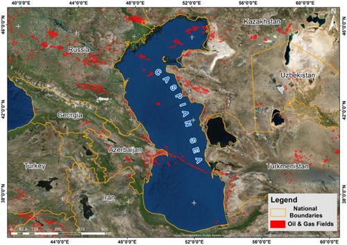
The Caspian Sea has considerable latitudinal extent and stretches across several climate zones: temperate continental climate to the north, temperate and warm on the western shore, subtropical on the southwestern and southern shores, and desert on the eastern shore (Zonn et al. 2010). The average annual air temperature above the Caspian Sea ranges from 10°C in the north to 17°C in the south. Variation in coastal topography drives variation in average annual precipitation over different parts of the Caspian Sea: 300 mm in the north, 300–600 mm in the west, 1600 mm in the southwest, 90 mm in the east and 200 mm over the Absheron Peninsula. The average annual wind speed over the surface of the Caspian Sea is 5.7 m/s. Current speeds are generally about 20–30 mm/s but can reach 100 mm/s near the Absheron Peninsula (Casp Info 2017).

3. Data processing

3.1. Satellite data sources and detection constraints

This research used both passive optical (LANDSAT) and active microwave (SENTINEL, RADARSAT, ENVISAT and ERS) satellite images to detect oil spills and natural seepage slicks. The use of both types of satellite data for this purpose is well established (Bentz and Barros 2005; Zhao et al. 2014).

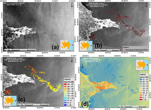
Data from both microwave SAR and passive optical sensors can be affected by environmental conditions. Passive optical sensors can only detect oil spills during daylight hours when clouds, fog or haze do not obscure the satellite’s view. SAR can detect oil slicks through clouds, and works equally well in darkness and daylight. However, SAR data are affected by wind and current speeds, sea temperature, the age of the slick, oil type and slick thickness (Ivanov et al. 2012). It is only possible to detect oil slicks when the wind speed is moderate (∼2.5–12.4 m/s) (Figure 2(a)) (Bayramov et al. 2016; Mityagina and Lavrova 2016). When the wind speed is lower than ∼2.5–3 m/s, the sea surface looks smooth regardless of whether an oil slick is present, and areas of low wind speed can be misinterpreted as oil slicks. It is especially difficult to detect thick oil slicks in low wind conditions. On the other hand, if the wind speed is more than ∼10–12.4 m/s, the sea surface becomes very rough regardless of whether oil is present, and it becomes very difficult to detect oil slicks, especially thin ones (Figure 2(b)). Figure 2(c,d) presents the reduction of the radar backscattering coefficient by an oil spill, which is the fundamental concept in the appearance of oil slicks as dark patches in the SAR images.

Figure 2. (a) Visible and (b) invisible oil slick because of wind speed; (c) radar backscattering of oil slicks and (d) backscattering of entire radar image (SENTINEL-1).

Of 931 archived satellite images acquired between 1996 and 2017, 411 were selected as useful for the detection of oil slicks. These 411 satellite images were acquired from SENTINEL, RADARSAT, ENVISAT, ERS and optical LANDSAT sensors, and were selected based on (1) ∼2.5–12.4 m/s wind speed range on the day the image was acquired and (2) visual inspection of image content for detection of oil spills and natural seepage slicks. Together, the images covered the entire area of the Caspian Sea with variable density (Figure 3, Table 1). This was considered as the main limitation of the research since this constrained the possibilities to perform more accurate and reliable computations of oil spill frequencies for the assessment of oil pollution hotspots and their sources. Due to the variable density of satellite image coverage, contextual information such as the locations of oil and gas platforms, wells, pipelines and vessel traffic was critical for this research to confirm the locations of oil pollution hotspots. Contextual information on oil and gas infrastructure, technology of platforms and wells, and their exploitation period may significantly contribute towards the understanding of man-made pollution sources.

Figure 3. Coverage of radar and optical satellite images in the Caspian Sea.

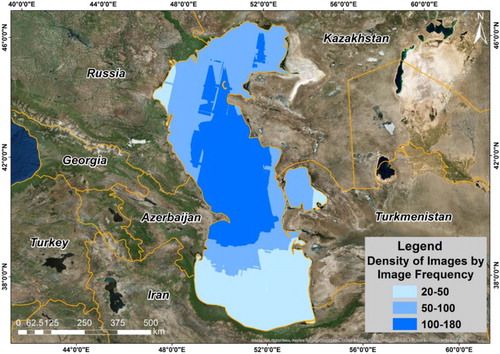
Table 1. Characteristics of satellite sensors and count of used satellite images.

Sensors	Mode	Resolution (m)	Swath width (km)	Band	Wavelength	Operative	Count of used images
SENTINEL-1	IW (Interferometric Wide)	20	250	C	3.75–7.5 cm	2014 – operating	12
RADARSAT-1	SCW (ScanSAR Wide)	100 × 100	450–500	C		1995 – operating	16
RADARSAT-2	SCW (ScanSAR Wide)	100 × 100	450–500	C		2007 – operating	10
ENVISAT	IM (Image Mode)	30 × 30	100	C		2002–2012	255
	WSM (Wide Swath Medium)	150 × 150	400				6
ERS-1	PRI (Precision Image Product)	30 × 30	100	C		1991–2000	20
ERS-2	PRI (Precision Image Product)	30 × 30	100	C		1995–2011	71
LANDSAT-5	TM (Thematic Mapper)	30	185	B1 – Blue, B2 – Green B3 – Red B4 - Near Infrared (NIR) B5 – Shortwave Infrared B6 – Thermal, B7 – Shortwave Infrared	B1 (0.45–0.52 µm) B3 (0.63–0.69 µm) B4 (0.76–0.90 µm) B5 (1.55–1.75 µm) B6 (10.40–12.50 µm) B7 (2.08–2.35 µm)	1984–2013	11
LANDSAT-8	OLI (Operational Land Imager)	30	185	B1 – Ultra Blue (coastal/aerosol) B2 – Blue B3 – Green B4 – Red B5 – Near Infrared B6 – Shortwave Infrared B7 – Shortwave Infrared B8 – Panchromatic B9 – Cirrus B10 – Thermal Infrared B11 – Thermal Infrared	B1 (0.435–0.451 µm) B2 (0.452–0.512 µm) B3 (0.533–0.590 µm) B4 (0.636–0.673 µm) B5 (0.851–0.879 µm) B6 (1.566–1.651 µm) B7 (2.107–2.294 µm) B8 (0.503–0.676 µm) B9 (1.363–1.384 µm) B10 (10.60–11.19 µm) B11 (11.50–12.51 µm)	2013 – operating	10

3.2. Detecting oil slick location and temporal repetition

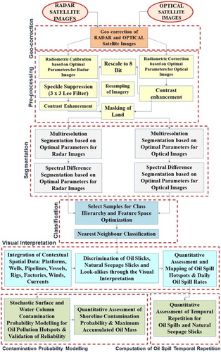
The workflow used for the semi-automatic detection of oil spills and seepage slicks, visual discrimination of oil slicks from look-alikes, computation of oil spill frequencies, approximation of leak sources and contamination probability modelling is presented in Figure 4. Several data-processing methods were used to optimise and standardise the data. Geo-correction of each individual satellite image was performed by geocoding relative to well-established geographic features within the research area. Radiometric calibration of SAR images was performed to restore original backscatter values, which can help reveal oil slicks and compare radar images acquired with different sensors or with the same sensor in different modes. A radiometric correction (Zhao et al. 2014) was applied to optical images to counteract atmospheric effects and simplify oil slick detection. The 3 × 3 Lee filter was used to remove speckles from radar images in order to improve processing and analysis (Sheng and Xia 1996; Arvelyna et al. 2001; Capstick and Harris 2001). This speckle function filters the speckled radar dataset and smooths out the noise while retaining the edges or sharp features in the image (Lee 1981). Contrast enhancement was applied to both radar and optical satellite images to improve the visibility of oil slicks. Finally, to optimise image processing time, all radar and optical images were rescaled to 8 bits and resampled to 50 m and land areas were masked.

Figure 4. Data-processing workflow for oil pollution studies in the Caspian Sea.

Multiresolution and spectral difference segmentation and classification of all 441 images were accomplished with eCognition software from Trimble (Topouzelis et al. 2002). Multiresolution segmentation accounts for spectrum, texture, shape and context to group pixels, partitioning a digital image into relatively homogeneous segments or objects. Spectral difference segmentation uses an algorithm that merges image segments or objects whose spectra differ by less than a given threshold to produce the final objects. Multiresolution and spectral difference segmentations were iteratively run and visually inspected to determine optimal parameters which would delineate major and minor oil slicks. Distinct parameters were used as optimal for segmentation of radar versus optical images (Table 2). The scale parameter controls the amount of spectral variability within objects and, therefore, their resultant size. The shape parameter controls the relative weighting of the object’s shape and its spectral colour. Compactness controls a weighting for representing the compactness of the objects formed during the segmentation. Further on, based on the generated segments, training samples of oil spills visually selected by operator from images, natural seepage slick, look-alike and water were collected for the class hierarchy. The iterative process of classification was run several times for each individual image with the addition of more training samples to improve the quality of classification to the greatest possible extent.

Table 2. Multiresolution and spectral difference segmentation parameters.

Multiresolution segmentation						Spectral difference segmentation
Scale parameter		Shape		Compactness		Maximum spectral difference
Radar	Optical	Radar	Optical	Radar	Optical	Radar	Optical
30	100	0.1	0.1	0.5	0.5	3	30

The segmentation and classification process identified dark spots, which could represent oil spills, natural seepage slicks or look-alikes. These three possibilities were then distinguished based on the characteristics of the dark spot and contextual information. Dark spot characteristics included shape, size/area, contrast, edge type, texture, duration and frequency of recurrence. Contextual information included wind and current speed, water depth, upwelling, eddies, atmospheric conditions (rain, dense fog and aerosols), river inflow, and direction and location of oil and gas pipelines, platforms and vessels.

Geospatial overlay segmentation analysis of the radar and optical satellite images was used to estimate the frequency with which oil spills and natural seepage spills recurred in the Caspian Sea. Clearly, estimates based on the selected 411 images collected over a 20-year period were not adequate to capture all or even most oil slicks occurring during that time. As mentioned before, to compensate for this gap, the role of contextual information relevant to marine petroleum and gas infrastructure was crucial for result validation. In addition, the kernel density method was used to generate an oil concentration heatmap for the Caspian Sea and verify oil spill and natural seepage hotspots identified from segmentation analysis. Areas of frequent oil spills (repetition <20) were identified, and this information, in combination with spatial information about petroleum and gas infrastructure, was used to identify the approximate locations of leak sources. Daily oil spill rates from oil and gas platforms at hotspots were calculated by multiplying computed areas of detected multi-year oil slicks by the thickness of the oil slick, which was estimated based on the sea surface colour from aerial observations in accordance with the Bonn Agreement Oil Appearance Standard (Table 3).

Table 3. Bonn agreement oil appearance codes (Bonn Agreement Aerial Operations Handbook 2009).

Appearance	Quantity (m^3/km^2)	Thickness (µm)	Typical appearance
Sheen (silvery/grey)	0.04–0.3	0.04–0.3
Rainbow	0.3–5	0.3–5
Metallic	5–50	5–50
Discontinuous true oil colour	50–200	50–200
Continuous true oil colour	>200	>200

3.3. Modelling and validation of water and shoreline contamination

The risk of water pollution and shoreline contamination from oil spills was modelled using Oil Spill Contingency and Response (OSCAR), the oil spill modelling software from SINTEF. OSCAR can perform deterministic and stochastic modelling of oil releases from platforms, rigs, vessels, wells, pipelines and other infrastructure and predict consequences for the water surface, water column, shoreline and coastal habitats (Ranjbar et al. 2014). OSCAR accounts for weathering of oil slicks as well as the physical, biological and chemical processes affecting oil at sea. Water and shoreline contamination was modelled for the period of 2006–2009 using spatiotemporal data of winds and currents developed by Imperial College London with a temporal resolution of 3 hours and provided with the OSCAR software package for the Caspian Sea (White and Toumi, 2013a, 2013b; Nicholls and Toumi 2014). Stochastic modelling was used to provide insight into the overall oil contamination probability under a wide range of weather conditions extrapolated from the multi-year dataset of Caspian Sea winds and currents. The oil contamination probability modelling was restricted to the period of 2006–2009 because the hydrodynamic data of winds and currents were only available for this period.

Estimated daily oil release rates (see Section 3.2) were one of the main inputs for contamination probability modelling. After the iterative runs of stochastic modelling, 30 simulations per year, with a 10-day duration for each simulation were selected as optimal in terms of two criteria: the reliability of modelling and processing time. Thirty simulations per year with run length of 10 days were considered optimal; a good balance of robustness of modelling results and processing time. The release temperature for oil spill hotspots was set to 20°C (Bayramov et al. 2016) and the water salinity to 12.5 ppt (Casp Info 2017). Since it is uncertain whether the oil leak sources are located on the top or bottom sides of marine oil and gas infrastructure, oil leaks were modelled on the sea floor. Model predictions were validated by comparing them to oil spills detected from multi-year 1996–2017 satellite images using spatial overlay and regression analysis.

Potential environmental consequences to the shoreline were assessed quantitatively using two metrics: shoreline contamination probability and maximum accumulated emulsion mass (tonnes). Shoreline contamination probability is the predicted likelihood that a particular segment of shoreline will be contaminated under different oil spill modelling scenarios. Maximum accumulated emulsion mass (tonnes) is an important factor for the iterative quantitative assessment of shoreline contamination based on shoreline habitat types and water contamination probability. Shoreline habitat types were mapped using object-based remote sensing analysis incorporating high-resolution multispectral Worldview-2 satellite images and ground-truth samples.

4. Results

4.1. Spatial distribution and repetition of man-made oil spills and natural seepage slicks in the Caspian Sea

Detection of oil slicks and classification into man-made and natural types (Figure 5) and computations of the temporal repetition and the kernel density-based heatmaps (Figures 6 and 7) revealed that man-made oil pollution and natural seepage slicks were spatially separate. The largest man-made oil spill hotspots were located near Oil Rocks Settlement, Pirallahi and Chilov Islands (Figures 6–8(b)). In contrast, natural oil slicks were most prevalent in the southern Caspian Sea (Figures 6 and 7).

Figure 5. Overall distribution of oil spills and natural seepage slicks in the Caspian Sea.

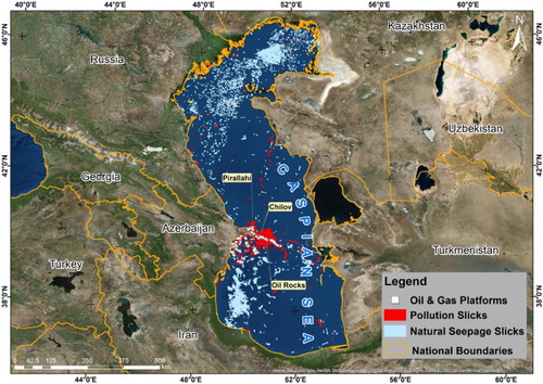
Figure 6. Temporal repetition (frequency) of oil spills and natural seepage slicks in the Caspian Sea.

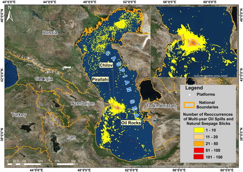
Figure 7. Heatmap of oil spills and natural seepage slicks in the Caspian Sea.

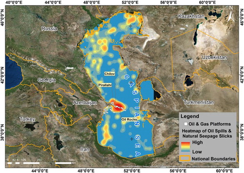
Figure 8. (a) Aerial view of the Oil Rocks Settlement; (b) Pirallahi and Chilov Islands; (c) repetition of oil spills associated with wells of Oil Rocks Settlement, Pirallahi and Chilov Islands and (d) sample aerial view of Bonn agreement oil appearance thickness codes (Bonn Agreement 2011).

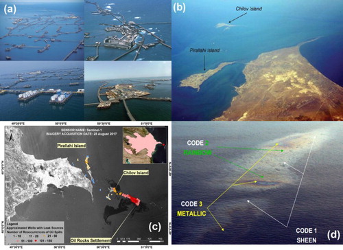
Areas around Oil Rocks Settlement, Pirallahi and Chilov Islands had different degrees of temporal repetition of oil spills (Figures 6 and 7). The largest area (5639 sq. km.) experienced 1–10 detected oil spills, while 993 km² experienced 11–20 oil spills, 775 km² experienced 21–50 oil spills, 208 km² experienced 51–100 oil spills and 36 km² experienced 101–150 oil spills. The highest frequency of oil leak sources was observed at Oil Rocks Settlement (Figure 8(c)).

The daily oil spill rate was calculated by multiplying the average area of detected oil spills around Oil Rocks Settlement, Pirallahi and Chilov Islands during 1996–2017 by its thickness. The estimated oil thickness for Oil Rocks Settlement was estimated from the studies of Ivanov et al. (2012) and Bonn Agreement Aerial Operations Handbook 2009 (Table 3, Figure 8(d)). Oil slicks present in the vicinity of Oil Rocks Settlement, Pirallahi and Chilov Islands had a ‘rainbow’ appearance, corresponding to a thickness of 0.3–5 μm. Thus, using an average oil spill area of 477 km², an oil spill volume range of 143 (477  × 0.3 μm) – 2385 (477 × 5 μm) m³ per day was estimated with a mean daily rate of 1264 m³. Although it is obvious that this is a significant range of oil spill volumes, it was decided to use the average equal to 1264 m³ as a daily oil spill rate since more accurate estimation of oil slick thickness was not possible without the availability of regular aerial observations.

4.2. Oil contamination probability modelling and validation

The probability of contamination around Oil Rocks Settlement, Pirallahi and Chilov Islands was modelled based on the computed approximate daily oil spill rate and four years (2006–2009) of wind and current data from the Caspian Sea developed by Imperial College London with a temporal resolution of 3 hours and provided with the OSCAR software package for the Caspian Sea (White and Toumi, 2013a, 2013b; Nicholls and Toumi 2014). The contamination risk for sea surface water, water column, shoreline and the total risk which combines the results of these three components from 2006 to 2009 was calculated (Figure 9(a–d)). The high-risk area had a distinctive triangular shape whether the surface, water column or total risk was considered (Figure 9(a–d)). This shape resulted from the interaction of numerous natural and anthropogenic factors, including Caspian Sea wind and current patterns, bathymetry and leak sources (Figure 10(a–d)). Wind speeds and directions are major factors which shape the currents in the Caspian Sea. The shape and topography of the seashore and seabed of the Caspian Sea also exert a substantial influence on the currents. It is well known that winds and currents affect the oil slick sizes and shapes. Much of the spatial variations of oil spills in different directions around the Oil Rocks Settlement, Chilov and Pirallahi Islands can be explained by patterns in the speed and direction of Caspian Sea currents (Bayramov et al. 2016).

Figure 9. (a) Water surface: probability of contamination (%); (b) water column: probability of contamination (%); (c) total contamination probability risk (%) and (d) graph of water surface, water column and total contamination probability.

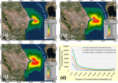
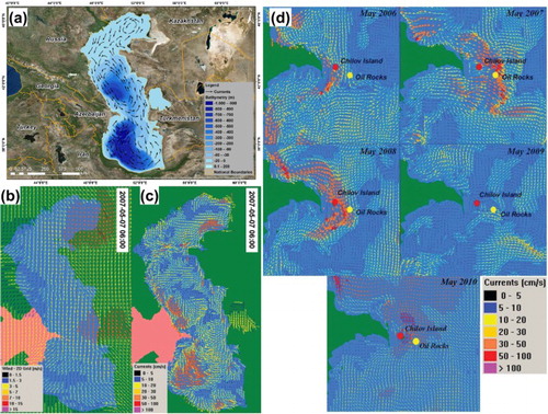
Figure 10. (a) Caspian Sea bathymetry and general circulation of currents; (b) detailed snapshots of Caspian Sea Winds; (c) currents visualised in OSCAR for date and time of 2007-05-07 06:00 and (d) currents around the Oil Rocks Settlement, Chilov and Pirallahi Islands.

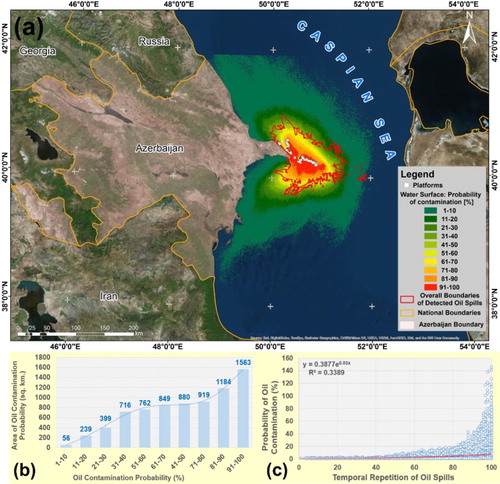
The majority (81% or 6157 km²) of sea surface area within the combined boundary of detected oil spills (7566 km²) had a 50% or greater chance of oil spill contamination (Figure 11(a,b)), indicating good agreement between predictions and data. Additionally, exponential regression analysis revealed a positive correlation between pixel values for contamination probability and calculated oil spill frequency with R² = 0.34 (Figure 11(c)).

Figure 11. (a) Cross-validation of predicted contamination probability with overall boundary of detected oil spills in the Caspian Sea; (b) distribution of predicted contamination probability classes within overall boundary of detected oil spills from satellite images and (c) exponential regression between probability of oil contamination and temporal repetition of detected oil spills from satellite images.

4.3. Quantitative assessment of shoreline contamination probability

The spatial variability in shoreline sensitivity to oil pollution was ranked on a scale from 1 to 10 based on environmental and social indicators, including biodiversity, the presence of protected areas, soil permeability and the presence of remediation activities. Shoreline sensitivity indexes from 1 to 10 were defined based on following three categories: shoreline type, biological and human-use resources (Figure 12(a)).

Figure 12. (a) Land-use classes along the shoreline of the Caspian Sea in Azerbaijan; (b) shoreline contamination probability (%) and (c) maximum accumulated emulsion mass (tonnes).

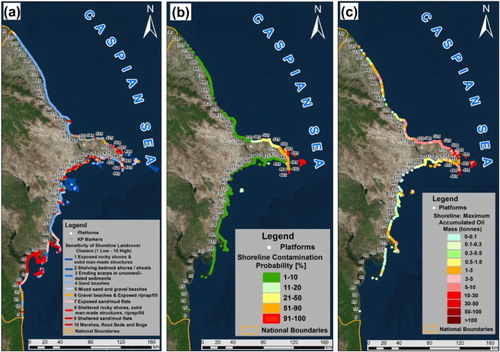
The threat that oil spills pose to Azerbaijan’s shoreline was assessed using two metrics: the probability of shoreline contamination and the predicted maximum accumulated emulsion mass. Shoreline contamination probability is a prediction of the likelihood that a given segment of shoreline will be contaminated under different oil spill modelling scenarios. Maximum accumulated emulsion mass is a key factor for the iterative quantitative assessment of shoreline contamination based on the shoreline habitat types, contamination probability of water and shoreline. Shoreline contamination probability was predicted for the period of 2006–2009 since it is based on the stochastic oil spill modelling results. The spatial resolution of habitat grids was set to 500 m × 500 m in the OSCAR software because it was optimal in terms of reliability, spatial coverage of modelling and processing time. Prediction of contamination probability along the shoreline of the Caspian Sea is presented in Figure 12(a). As it is possible to observe in Figures 12(b) and 13(a), the contamination probability of more than 50% was primarily located in the shoreline range of 464–508 km with the existence of high rank environmental and social sensitivities in this range. The highest probability of contamination was predicted for the 16.5 km length of sand beaches and 8 km length of marshes, reed beds and bogs (Figure 13(b)).

Figure 13. (a) Kilometre range of environmental sensitivities and contamination probability; (b) distance of land-use classes within contamination probability >50%; (c) kilometre range of maximum accumulated emulsion mass (tonnes); (d) distance of predicted maximum accumulated emulsion mass within contamination probability > 50%; (e) validation of shoreline contamination probability with shoreline pollution frequency detected from satellite images.

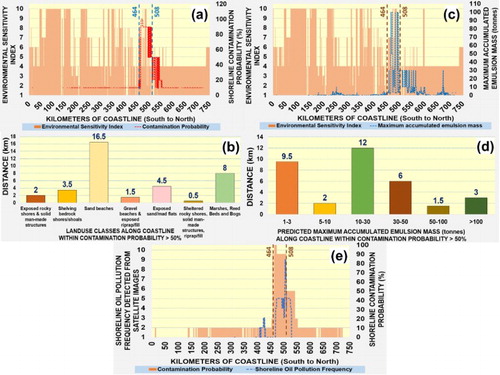
Prediction of potential maximum accumulated emulsion mass (tonnes) along the shoreline of the Caspian Sea is presented in Figure 12(c). The highest maximum accumulated emulsion mass (tonnes) can also be observed in the shoreline range of 464–508 km with high contamination probability >50% and with the existence of high rank environmental and social sensitivities (Figure 13(c)). The prediction of the highest maximum accumulated emulsion mass (tonnes) covered 9.5 and 12 km of shoreline for 1–3 and 10–30 classes of maximum accumulated emulsion mass (tonnes), respectively (Figure 13(d)).

Verification of shoreline contamination predictions based on the frequency of detected oil slicks at the shoreline of the Caspian Sea using satellite images showed that 32 out of 44 km predicted shoreline with contamination probability >50% was affected by oil pollution occurrences (Figure 13(e)).

5. Conclusions

1. The spatial and temporal occurrence of oil spills and natural seepage slicks in the Azerbaijani portion of the Caspian Sea was assessed using 411 SAR and optical satellite images from 1996 to 2017. The anthropogenic oil spills with the largest spatial extent and most frequent occurrence were located around Oil Rocks Settlement, Pirallahi and Chilov Islands, while natural seepage slicks were most prevalent in the southern part of the Caspian Sea. The biggest hotspot of oil spills and leak sources were observed at Oil Rocks Settlement with computed temporal repetition of oil spills equal to 51–100 (208 sq. km), 101–150 (36 sq. km) and oil leak frequencies of wells equal to 51–100 (39), 101–150 (127). The average daily oil spill rate at the Oil Rocks Settlement, Pirallahi and Chilov Islands was estimated to be 1264 m³.

2. A triangular area (7566 km²) characterised by high risk of oil contamination was identified immediately offshore of the Absheron Peninsula, where the Azerbaijani capital, Baku, is located. The size, shape and location of this area result from the interaction of natural and anthropogenic factors, including wind and current speed and direction, bathymetry, and primary leak sources on the sea floor. Eighty-one per cent (6157 of 7566 km²) of the entire study area had a 50% or greater chance of contamination over 2006–2009 periods. Pixel values for the modelled risk of contamination were positively correlated with the observed frequency of oil spills during the study period, supporting the reliability of the modelling approach.

3. The contamination probability more than 50% was primarily located in the shoreline range of 464–508 km with the existence of high rank environmental and social sensitivities in this range. The highest probability of contamination was predicted for the 16.5 km length of sand beaches and 8 km length of marshes, reed beds and bogs. The highest maximum accumulated emulsion mass (tonnes) was also observed in the shoreline range of 464–508 km with high contamination probability >50% and with the existence of high rank environmental and social sensitivities. The predictions covered 9.5 km and 12 km of shoreline for 1–3 and 10–30 classes of maximum accumulated emulsion mass (tonnes), respectively. Verification of shoreline contamination predictions based on the frequency of detected oil slicks at the shoreline of the Caspian Sea using satellite images showed that 32 out of 44 km predicted shoreline with the contamination probability >50% was affected by oil pollution occurrences.

Acknowledgements

We acknowledge European Space Agency (ESA – Project ID: 15837) for providing access to satellite images to implement this research. A Fulbright Scholar fellowship to Dr. Emil Bayramov supported the collaboration between three authors.

Disclosure statement

No potential conflict of interest was reported by the authors.

References

- Akar S, Lutfi Süzen M, Kaymakci N. 2011. Detection and object-based classification of offshore oil slicks using ENVISAT-ASAR images. Environ Monitor Assess. 183:409–423. doi: 10.1007/s10661-011-1929-6
- Arvelyna Y, Oshima M, Kristijono A, Gunawan I. 2001. Auto segmentation of oil slick in Radarsat SAR image data around Rupat Island Malacca Strait. Proceedings of ACRS 2001, 22nd Asian Conference on Remote Sensing; 2001 Nov 5–9. Centre for Remote Imaging, Sensing and Processing (CRISP); Singapore: National University of Singapore.
- Bayramov E, Buchroithner M, Bayramov R. 2016. Multi-temporal assessment of ground cover restoration and soil erosion risks along petroleum & gas pipelines in Azerbaijan using GIS and remote sensing. Environ Earth Sci. 75:256. doi: 10.1007/s12665-015-5044-9
- Bentz CM, Barros JO. 2005. A multi-sensor approach for oil spill and sea surface monitoring, in southeastern Brazil. International Oil Spill Conference Proceedings; p. 703–706.
- Brekke C, Solberg AHS. 2005. Oil spill detection by satellite remote sensing. Remote Sens Environ. 95:1–13. doi: 10.1016/j.rse.2004.11.015
- Bonn Agreement. 2011. BAOAC Photo Atlas (Bonn Agreement Oil Appearance Code). http://www.bonnagreement.org/publications.
- Bonn Agreement Aerial Operations Handbook. 2009. [accessed 2017 Feb. 6]. http://www.bonnagreement.org/publications.
- Capstick D, Harris R. 2001. The effects of speckle reduction on classification on ERS SAR data. Int J Remote Sens. 18:3627–3641. doi: 10.1080/01431160110056506
- Casp Info. 2017. [accessed 2017 Feb. 6]. http://www.caspinfo.net/.
- Del Frate F, Petrocchi A, Lichtenegger J, Calabresi G. 2000. Neural networks for oil spill detection using ERS-SAR data. IEEE Trans Geosci Remote Sens. 5:2282–2287. doi: 10.1109/36.868885
- Espedal HA. 1998. Detection of oil spill and natural film in the marine environment by spaceborne synthetic aperture radar [PhD thesis]. Bergen: Department of Physics University of Bergen and Nansen Environment and Remote Sensing Center.
- Espedal HA, Johannessen OM. 2000. Detection of oil spills near offshore installations using synthetic aperture radar (SAR). Int J Remote Sens. 21:2141–2144. doi: 10.1080/01431160050029468
- Espedal HA, Wahl T. 1999. Satellite SAR oil spill detection using wind history information. Int J Remote Sens. 20:49–65. doi: 10.1080/014311699213596
- Friedman KS, Pitchel WG, Clemente-Colon P, Li X. 2002. GoMEx – an experimental GIS system for the Gulf of Mexico Region using SAR and additional satellite and ancillary data. International Geoscience and Remote Sensing Symposium, IGARSS ‘02. 2002 IEEE International. doi:10.1109/IGARSS.2002.1027177.
- Gade M, Scholz J, von Viebahn C. 2000. On the detectability of marine oil pollution in European marginal waters by means of ERSSAR imagery. Proceedings IGARSS 2000; 2000 Jul 24–28. Honolulu, HI: IEEE.
- Girard-Ardhuin F, Mercier G, Garello R. 2003. Oil slick detection by SAR imagery: Potential and limitation. IEEE/MTS Proceedings of the Marine Technology and Ocean Science Conference OCEANS2003; 2003 Sep 2226; San Diego, CA: IEEE.
- Ivanov AY, Dostovalov MY, Sineva AA. 2012. Characterization of oil pollution around the oil rocks production site in the Caspian Sea using spaceborne polarimetric SAR imagery. Izvestiya Atmos Oceanic Phys. 48:1014–1026. doi: 10.1134/S0001433812090058
- Ivanov AY, Fang M, He M-X, Ermoshkin IS. 2004. An experience of using Radarsat, ERS-1/2 and Envisat SAR images for oil spill mapping in the waters of the Caspian Sea, Yellow Sea and East China Sea. Envisat and ERS Symposium; 2004 Sep 6–10; Salzburg, Austria (ESA SP-572).
- Ivanov AY, Kucheiko AA. 2016. Distribution of oil spills in inland seas based on SAR image analysis: a comparison between the Black Sea and the Caspian Sea. Int J Remote Sens. 37(9): 2101–2114. doi: 10.1080/01431161.2015.1088677
- Ivanov AY, Vostokov SV, Ermoshkin IS. 2004. Mapping oil films on the sea surface using synthetic aperture radar images (the Caspian Sea as an example). Earth Observation Space. 4:82–92. [In Russian.]
- Ivanov AY, Zatyagalova VV. 2008. A GIS approach to mapping oil spills in a marine environment. Int J Remote Sens. 29:6297–6313. doi: 10.1080/01431160802175587
- Jha MN, Levy J, Gao Y. 2008. Advances in remote sensing of oil spill disaster management: state-of-the-Art sensor technology for Oil spill surveillance. Sensors. 8:236–255. doi: 10.3390/s8010236
- Karantzalos K, Argialas D. 2008. Automatic detection and tracking of oil spills in SAR imagery with level set segmentation. Int J Remote Sens. 29:6281–6296. doi: 10.1080/01431160802175488
- Kotova LA, Espedal HA, Johannessen OM. 1998. Oil spill detection using spaceborne SAR; a brief review. Proceedings of 27th ISRSE; Tromsb, Norway.
- Kubat M, Holte RC, Matwın S. 1998. Machine learning for the detection of oil spills in satellite radar images. Machine Learn. 2–3:195–215. doi: 10.1023/A:1007452223027
- Lee JS. 1981. Speckle analysis and smoothing of synthetic aperture radar images. Comput Graphics Image Process. 17:24–32. doi: 10.1016/S0146-664X(81)80005-6
- Leifer I, Luyendyk B, Broderick K. 2006. Tracking an oil slick from multiple natural sources, coal oil point, California. Marine Petroleum Geol. 23:621–630. doi: 10.1016/j.marpetgeo.2006.05.001
- Li X, Pichel W, Cheng Y, Garcia-Pineda O, Liu P, Streett D, Gallegos S. 2010. Oil spill response utilizing SAR imagery in the Gulf of Mexico. Proceedings of SEASAR 2010 Workshop; 2010 Apr 1; Frascati.
- Lu J. 2003. Marine oil spill detection, statistics and mapping with ERS SAR imagery in Southeast Asia. Int J Remote Sens. 24:3013–3032. doi: 10.1080/01431160110076216
- Lu J, Lim H, Liew SC, Bao M, Kwoh LK. 1999. Ocean oil pollution mapping with ERS synthetic aperture radar imagery. Proceedings of IGARSS ‘99; 1999 Jun 28–Jul 02; Hamburg: IEEE.
- Marghany M, Hashim M. 2011. Discrimination between oil spill and look-alike using fractal dimension algorithm from RADARSAT-1 SAR and AIRSAR/POLSAR data. Int J Phys Sci. doi:10.5772/5747747.
- Marghany M, Mansor S. 2015. Genetic algorithm for oil spill automatic detection using synthetic aperture radar. Global NEST J. 17(4):858–869.
- Martinez A, Moreno V. 1996. An oil spill monitoring system based on SAR images. Spill Sci Technol Bull. 3(1/2):65–71. doi: 10.1016/S1353-2561(96)00025-4
- Mityagina M, Lavrova O. 2016. Satellite survey of inner seas: oil pollution in the Black and Caspian Seas. Remote Sens. 8:875. doi: 10.3390/rs8100875
- Nicholls JF, Toumi R. 2014. On the lake effects of the Caspian Sea. Q J R Meteorol Soc. 140(681):1399–1408. doi: 10.1002/qj.2222
- O’Brein GW, Lawrence GM, Williams AK, Glenn K, Barrett AG, Lech M, Edwards DS, Cowley R, Boreham CJ, Summons RE. 2005. Yampi shelf, browse basin, North-West Shelf, Australia: a test-bed for constraining hydrocarbon migration and seepage rates using combinations of 2D and 3D seismic data and multiple, independent remote sensing technologies. Marine Petroleum Geol. 22:517–549. doi: 10.1016/j.marpetgeo.2004.10.027
- Ranjbar P, Shafieefar M, Rezvandoust J. 2014. Modeling of oil spill and response in support of decreasing environmental oil effects case study: blowout from Khark Subsea Pipelines (Persian Gulf). Int J Environ Res. 8(2):289–296.
- Sheng Y, Xia Z. 1996. A comprehensive evaluation of filters for radar speckle suppression. Proceedings of the International Geoscience and Remote Sensing Symposium IGARSS’96; 1996 May 27–31. Lincoln, NE: IEEE.
- Solberg AHS, Storvik G, Solberg R, Volden E. 1999. Automatic detection of oil spills in ERS SAR images. IEEE Trans Geosci Remote Sens. 37:1916–1924. doi: 10.1109/36.774704
- Topouzelis KN. 2008. Oil spill detection by SAR images: dark formation detection, feature extraction and classification algorithms. Sensors. 8:6642–6659. doi: 10.3390/s8106642
- Topouzelis K, Karathanassi V, Pavlakis P, Rokos D. 2002. Oil spill detection: SAR multi-scale segmentation and object features evaluation. In Bostater and Santoleri, editors. 9th International Symposium on Remote Sensing (SPIE, 4880); 2002 Sep 23–27. Creta, Greece; p. 77–87.
- Topouzelis K, Muellenhoff O, Ferraro G, Tarchi D. 2007. Satellite mapping of oil spills in the East Mediterranean Sea. Proceedings of the 10th International Conference on Environmental Science and Technology; 2007 Sep 5–7; Greece: Kos Island.
- White RH, Toumi R. 2013a. River flow and ocean temperatures: The Congo River. J Geophys Res Oceans. 119(4):2501–2517. doi: 10.1002/2014JC009836
- White RH, Toumi R. 2013b. The limitations of bias correcting regional climate model inputs. Geophys Res Lett. 40(12):2907–2912. doi: 10.1002/grl.50612
- Xing Q, Li L, Lou M, Bing L, Zhao Z. 2015. Observation of oil spills through Landsat thermal infrared imagery: a case of deepwater horizon. Aquat Procedia. 3:151. doi: 10.1016/j.aqpro.2015.02.205
- Zatyagalova VV, Ivanov AY, Golubov BN. 2007. Application of Envisat SAR imagery for mapping and estimation of natural oil seeps in the South Caspian Sea. In Lacoste H, Ouwehand L, editors. Proceedings of the Envisat Symposium-2007; 2007 Apr 23–27; Montreux (ESA SP-636), CD-ROM. Noordwijk: ESA Publication Division.
- Zhao J, Temimi M, Ghedira H, Hu C. 2014. Exploring the potential of optical remote sensing for oil spill detection in shallow coastal waters-a case study in the Arabian Gulf. Opt Express. 22:13755–13772. doi: 10.1364/OE.22.013755
- Ziemke T. 1996. Radar image segmentation using recurrent artificial neural networks. Pattern Recogn Lett. 4:319–334. doi: 10.1016/0167-8655(95)00128-X
- Zodiatis G, Lardner R, Solovyov D, Panayidou X, De Dominicis M. 2012. Predictions of oil slicks detected from satellite images using MyOcean forecasting data. Ocean Sci. 8:1105–1115. doi: 10.5194/os-8-1105-2012
- Zonn IS, Kosarev AN, Glantz M, Kostianoy AG. 2010. The Caspian Sea Encyclopaedia. 2010 ed. Berlin: Springer.