A comparison of scatterometer and HF radar wind direction measurements

ABSTRACT

Scatterometer winds are increasingly being used by Meteorological Services to validate and assimilate into their forecast models and reanalyses. In this paper, ASCAT wind directions obtained in coastal regions around Australia are compared with those derived from ground-based HF radar systems. Good agreement is demonstrated at wind speeds greater than 5 m/s. At lower wind speeds, scatterometer winds are not expected to be as accurate and the HF radar is probably measuring swell rather than wind direction. Examples are presented that demonstrate the advantage for regional coastal wind and wave modelling of the higher temporal resolution available with the HF radar which enables tracking of frontal features.

KEYWORDS:

• HF radar
• wind direction
• scatterometer
• ASCAT
• coastal winds
• IMOS
• ACORN

1. Introduction

HF radars for oceanographic applications are normally located on the coast and transmit radio waves out to sea that are scattered from ocean waves generating a received signal which is Doppler shifted by the motion of the waves. The amplitude and Doppler shifts can be analysed to provide measurements of surface currents, waves and winds (Wyatt 2014). These systems are increasingly being used for operational coastal monitoring of surface currents with many systems now being located around the coasts of the USA (Harlan et al. 2010), Japan (Ebuchi et al. 2006), China (Zhao et al. 2011), Australia (Heron and Prytz 2011), Europe (Rubio et al. 2017) and other parts of the world. The wave and wind measurements are not yet seen as operational products although there are many publications that demonstrate these capabilities (Wyatt et al. 2003, 2006, 2011; Lipa and Nyden 2005; Wyatt 2012). Wind direction is obtained from the same part of the signal used to measure surface currents whereas waves and wind speed use much lower amplitude signals and are thus more likely to be influenced by noise or non-wave (e.g. ship) contributions to the signal.

This paper focusses on wind direction measurements obtained using the method described in Wyatt et al. (1997) and implemented in software provided by Seaview Sensing Ltd. Examples are given of data obtained from the Australian Integrated Marine Observing System (IMOS), Coastal Ocean Radar Network (ACORN, Wyatt 2015) WERA HF radars (Gurgel et al. 1999). These data are compared with 12.5 km ASCAT scatterometer winds obtained from the European Organization for the Exploitation of Meteorological Satellites (EUMETSAT). As far as the author is aware this is the first such comparison and one aim of this paper is to show the potential value of HF radar data as another source of information to validate scatterometer algorithms. Of course the paper can also be viewed as a validation of the HF radar measurements using scatterometer winds and this was an original aim. However, as discussed in the next section, there appear to have been more detailed validations of HF radar wind directions with in situ instruments and models than has been the case for scatterometer winds giving more confidence in the HF radar outputs except in low winds when both methods are known to be less accurate.

To date, no one has published a robust wind speed algorithm for use with HF radar data. The Seaview Sensing software provides wind speed using the method of Dexter and Theodorides (1982) which is an inverse wind wave modelling approach, and, as such, only suitable when all the wave energy is locally wind generated. As already mentioned, this measurement uses low amplitude parts of the HF radar signal which can be influenced by noise, imperfections in, or poor calibrations of, the receive antenna system, ship signals, interference, etc. and as a result spatial coverage is much more limited than is the case for wind directions and the information provided is not currently promoted as a robust product.

Wind directions on their own do have some operational value. For example, the Australian Bureau of Meteorology in South Australia, an area which is very susceptible to serious bush fire events, is particularly interested in offshore wind direction data since this has the potential to improve bush fire modelling on land. In addition, they can be used to validate the measurements from other instruments and, in particular in the context of this paper, satellite scatterometry measurements.

The next section presents the data and methods used. This is followed by a presentation of and discussion on the results. Finally concluding remarks are presented.

2. Data and methods

At the time of writing, there are four WERA dual HF radar sites in Australia which will be referred to as follows: CBG (Capricorn Bunker Group at the southern end of the Great Barrier Reef off the Queensland coast), COF (Coffs Harbour, off the northern NSW coast), SAG (South Australian Gulfs, SW of Adelaide in South Australia) and ROT (seas around Rottnest Island off the coast near Perth, WA). These sites and the radar locations can be seen in figures presented in Section 3. The radars at CBG, ROT and SAG operated at frequencies of 8.34, 8.51 and 8.51 MHz respectively with a measurement grid with spacing of 4.5 km whereas the COF radars operated at 13.92 MHz with a grid spacing of 1.5 km.

Wind direction measurements are not made operationally but a few years of archived data at each of these sites have been processed to obtain both wave and wind data. Six consecutive months of data at each site have been used for this study. These are SAG, April to September 2011; CBG and ROT, January to June 2014; COF, November 2013 to April 2014. They were the latest available data sets in each case. Wind directions are obtained from the relative amplitude of the two peaks in the radar power (Doppler) spectrum. These correspond to Bragg scatter from linear ocean waves with half the radio wavelength. At the radio frequencies used, 8.34, 8.51, 13.92 MHz, these waves have frequencies of 0.295, 0.298 and 0.382 Hz respectively and are assumed to be aligned with the local wind except in low seas. The Seaview Sensing measurement (Wyatt et al. 1997) is a maximum likelihood fit of a two parameter directional model of these short waves (the sech model, Donelan et al. 1985), the parameters being direction and directional spreading.

NetCDF files containing ASCAT coastal 12.5 km swath grid wind data (Verhoef et al. 2012), for the selected periods and for the regions covered by the CBG, COF and ROT HF radars, were obtained from EUMETSAT (EO:EUM:DAT:METOP:OSI-104 © EUMETSAT). The available SAG radar data was from 2011 and the corresponding ASCAT data were obtained from the JPL PODAAC since they are not available in NetCDF form at EUMETSAT. The original aim of this work was to use these data to validate the HF radar data but, after reviewing the available and rather sparse literature on scatterometer wind direction validation, this work could also be viewed as a validation of the scatterometer data using the HF radar, in particular because there have been very few such validations in the southern hemisphere where very long fetches could introduce a bias due to swell. Verhoef et al. (2012) validated these winds first against the previous ASCAT 12.5 km product which was more limited in coastal regions and second using a large number of collocated buoys although only one of these was south of S. They presented wind speed and wind component statistics but not wind directions. Wind direction statistics have been presented in Rani et al. (2014), Wu and Chen (2015) and Bentamy et al. (2008). The first two provide standard formulae for determining root mean square (rms) difference which they apply to the wind direction comparisons but they do not make it clear whether they have accounted for directions on either side of although presumably they did. Wu and Chen (2015) find biases of and rms differences of reducing to for wind speeds in the range 5–15 m/s. Rani et al. (2014) found seasonal and regional differences in their statistics with rms differences ranging from 14 to 21. Bentamy et al. (2008) refer to a standard deviation difference and vector correlation without stating how these have been determined. For the buoy comparison, a standard deviation of was found which reduced to for wind speeds from 5 to 10 m/s and for higher wind speeds. It is unclear how to interpret the vector correlations given since they are greater than 1.

For the statistical comparison presented here, the HF radar and scatterometer measurements were required to be no more than half an HF radar range cell width (i.e. 750 m at COF and 2.25 km elsewhere) and 30 minutes apart. Three statistical methods are used: (a) the mean difference, its 95% confidence interval and concentration (Bowers et al. 2000); (b) the circular correlation coefficient (Fisher and Lee 1983; Fisher 1993); (c) the vector correlation and phase difference (Kundu 1976) noting that the phase difference and mean differences should be equal. Note that since only wind direction is available from the HF radar data, it is only direction that is compared and is regarded as a vector with magnitude one where this is needed for the analysis. Maps are presented to show examples of good and bad agreements and support the discussion. Previous validations of HF radar wind directions include comparisons with coastal wind measurements (Wyatt 2012) (biases of 7.4–11.7, rms of 39.2–48 and circular correlations of .58–.68), with Quickscat (Wyatt et al. 2006) (bias of , rms of ) and model winds (Wyatt et al. 2006) (bias of , rms of and circular correlation of 0.89).

3. Results

3.1. Scatter plots and statistics

Figure 1 shows scatter plots of the comparisons at all four sites, the statistics of which are given in Table 1. The plot has been colour coded using the scatterometer wind speeds and it is clear that the biggest differences are when this speed is low. This is consistent with previous studies of ASCAT winds and may also be linked to the HF radar requirement that Bragg waves be wind driven. Table 1 also includes the statistics calculated when a low wind speed threshold of 5 m/s is set confirming the improved agreement at higher wind speeds. Other possible drivers for difference that were examined are location of the HF radar measurement site and directional spreading measured by the HF radar. The former was used because HF radar signals decrease in magnitude at longer distances from the radars introducing more noise into the measurements and they may also be contaminated by sidelobes towards the azimuthal extremes of coverage; the latter because high directional spreading (as will be seen below) seems to indicate the presence of meteorological or oceanographic frontal systems which may not be seen by the scatterometer. However, neither of these seemed to be obviously affecting the outcome of the comparison. Figure 2 presents the data in the form of a histogram and shows that most of the data are in good agreement as is also clear from the statistics.

Figure 1. Scatter plots of scatterometer and HF radar wind directions. The colour coding is scatterometer wind speed in m/s.

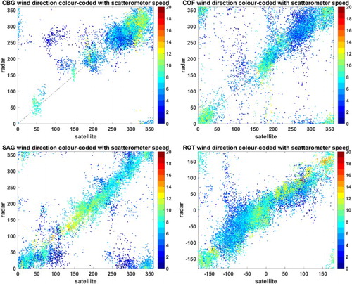
Figure 2. Histograms of scatterometer and HF radar wind directions. The colour coding is percentage of observations in each bin where the maximum on the scale is set at the maximum percentage in any bin. For clarity bins with of the maximum are not shown.

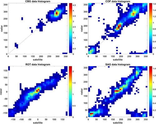
Table 1. Statistics of the comparisons.

Statistic	CBG		COF		ROT		SAG
Number of data pairs	12,889	11,192	9378	7058	20,299	18061	9961	8426
Direction difference	−7.55	−8.13	10.76	8.08	7.02	6.80	3.76	3.33
95% confidence interval	0.51	0.43	0.74	0.68	0.43	0.39	0.69	0.56
concentration	4.30	6.71	3.04	4.37	4.33	5.09	3.21	5.30
Complex correlation	0.87	0.92	0.81	0.88	0.86	0.90	0.83	0.90
phase difference	−7.55	−8.13	10.76	8.08	7.02	6.90	3.76	3.33
circular correlation	0.62	0.68	0.66	0.76	0.74	0.80	0.68	0.79

Note: Figures in bold italics are after 5 m/s wind speed thresholding.

3.2. Spatial comparisons

Figure 3 shows maps of HF radar and scatterometer measurements at a time of higher wind speeds where agreement is generally good. The scatterometer winds are within 30 minutes of the HF radar measurement. The arrows are proportional to wind speed but the scaling is different at each location. Figure 3(a) shows scatterometer winds from ENE over most of the CBG region with a similar pattern seen in the HF radar data although there are small differences in direction in some places. The COF map, Figure 3(b), shows winds from the north in both scatterometer and HF radar data. There are some obvious differences in the south-east where the HF radar directions are backing from northerly to a more north-westerly direction. Although this could be a real feature, confidence in the HF radar wind measurements is more limited at longer ranges where signal-to-noise is near the allowed threshold. Wind directions are well aligned in Figure 3(c) from ROT and mostly in Figure 3(d) from SAG although there are small differences in the southern part of the coverage. Again there may be signal-to-noise limitations in the HF radar data here.

Figure 3. Maps showing HF radar wind direction (black arrows) and directional spreading (colour-coded) with scatterometer winds (red arrows). The map for ROT (c) includes data from both Metop-A and -B. HF radar sites are labelled and marked with . Blue lines are depth contours.

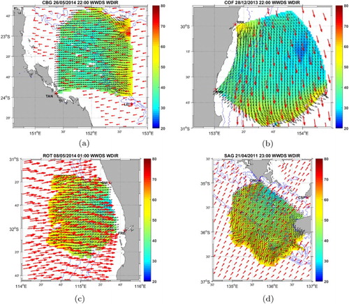
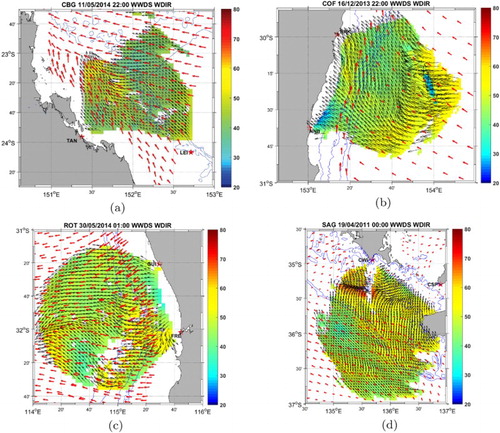
Figure 4 shows examples with more spatial variability in the wind fields. Figure 4(a) shows scatterometer winds from ESE in the northern part of the CBG region with winds from a more southerly direction on most of the shelf. A similar pattern is seen in the HF radar data although there are small differences in direction over most of the region. Figure 4(b) shows winds from the SE veering to a more southerly direction to the north-east of the region. The veering is more marked in the scatterometer data and is associated with much higher wind speeds along the shelf edge. The HF radar data do not show the same veering in the south-west part of the region. The ROT example, Figure 4(c), shows generally offshore winds with some variation in direction in the scatterometer winds but rather more in the HF radar winds so some areas where the differences are quite large, for example in the south-west of the region. In Figure 4(d), offshore winds are from the SE as seen in both measurements. Closer to the coast, the scatterometer is indicating much lower wind speeds and the HF radar wind directions are veering towards the NE. In such low winds, it is possible that the HF radar is actually measuring the direction of swell waves coming onto the shelf.

Figure 4. Maps showing HF radar wind direction (black arrows) and directional spreading (colour-coded) with scatterometer winds (red arrows). The map for ROT (c) includes data from both Metop-A and -B. HF radar sites are labelled and marked with . Blue lines are depth contours.

The temporal and spatial variations in the directional spreading measured by the HF radar have not been mentioned so far. It is not the main focus of this paper and has not yet been studied in great detail. However there is some evidence that, together with the wind direction measurements, spreading can be used to detect meteorological fronts (Heron et al. 2016) and other changing weather conditions. Figure 5 seems to show a region of wind direction convergence and high directional spreading moving across the HF radar coverage region from west to east over a period of 9 hours. The scatterometer data can be seen in Figure 5(g,h) and shows reasonable agreement with the HF radar data to the west of the convergence region where wind speeds are higher. To the east of this region, the two systems measure rather different directions but it should be noted that wind speeds are low here. Archived Australian Bureau of Meterology surface pressure charts have been used to interpret these maps. These measurements were made during a period when the centre of a high pressure region was moving slowly from the coast to the east just to the north of the radar measurements so this is clearly not a meteorological front. In this example, it is likely that the offshore winds are increasing slightly as the high moves offshore, enough to generate wind waves that are detectable by the radar. The measurements further offshore are more likely to be associated with swell from a low pressure system north-west of New Zealand which might explain the differences from the scatterometer directions. Another example is shown in Figure 6. In this case, the meteorological charts show a low with an associated trough centred just to the north of the radar measurement region at 12:00 UTC moving to the south-east by 18:00 with offshore winds ahead of the low and onshore winds behind. Another example with a frontal signature is seen in Figure 7 although in this case the directional spreading is not as high along the front which can be seen running roughly from north to south in the centre of Figure 7(a). Ahead of the front winds are from the north-east with an anti-clockwise rotation associated with high pressure to the east. Behind the front winds are from the north-west or west depending on the exact position of the front. The scatterometer winds seen in the last panel, Figure 7(f), are consistent with the HF radar wind directions. Note that in these examples all available scatterometer data have been included; HF radar data is available with higher temporal resolution. Many other examples of wind (or wave) direction convergence have been seen in the data.

Figure 5. (a–i) Hourly (16:00 UTC 06/12/2013 to 00:00 07/12/2013) maps showing HF radar wind direction (black arrows) and directional spreading (colour-coded) with scatterometer winds (red arrows) during the movement of a high from west to east north of the site in central east Australia. Radar sites are labelled and marked with . Blue lines are depth contours. (j–l) Surface pressure charts at 12:00, 18:00 and 00:00.

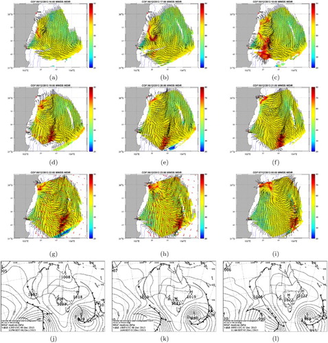
Figure 6. (a–c) Six-hourly maps (12:00 UTC 26/04/2014 to 00:00 27/04/2014) showing HF radar wind direction (black arrows) and directional spreading (colour-coded) before, during and after the passage of a low pressure system moving from north-west to south-east across SW Australia. Radar sites are labelled and marked with . Blue lines are depth contours. (d–f) Surface pressure charts at the corresponding times.

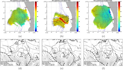
Figure 7. (a–f) Hourly maps (08:00 UTC to 13:00 08/04/2011) showing HF radar wind direction (black arrows) and directional spreading (colour-coded) with scatterometer winds (red arrows) before, during and after the passage of a cold front associated with a low pressure system moving from west to east with high pressure to the east across central South Australia. Radar sites are labelled and marked with . Blue lines are depth contours. (g–h) Surface pressure charts at 06:00 and 12:00.

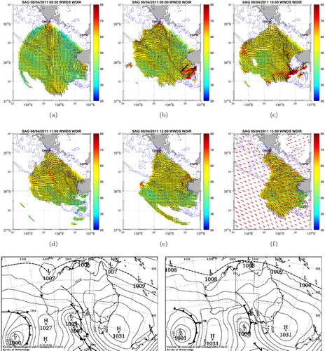
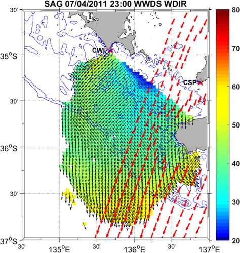
Figure 8 is another example showing the potential value of the HF radar directional spreading measurement. In this case, there are strong unidirectional offshore winds and the figure shows the development of increased directional spreading with fetch.

Figure 8. Map showing HF radar wind direction (black arrows) and directional spreading (colour-coded) with scatterometer winds (red arrows) for a fetch-limited case at SAG. HF radar sites are labelled and marked with . Blue lines are depth contours.

4. Concluding remarks

This paper has shown that scatterometer and HF radar wind directions are generally in good agreement, comparable with previous studies, but with some differences. We have not attempted to identify all the sources of difference although wind speed is clearly a factor. In the case of the radar, a low wind speed means that the measurements are more likely indicating swell rather than wind direction and the scatterometer measurements are known to be less reliable in these conditions. The scatterometer winds are generally more uniform spatially than the radar winds, for example see Figure 8, where the radar winds are aligned with the scatterometer over part of the region but there are differences to the south. These regions of difference are at the outer bounds of the radar coverage so are possibly an indication of poor signal to noise influencing the radar measurements. Or there could be something in the scatterometer processing which encourages spatial consistency. Some measurements together with in situ instruments would help to resolve these questions.

The radar measurements are clearly of higher resolution temporally and spatially albeit with variable overall coverage. The coverage of the particular HF radar measurement regions referred to here by the scatterometer is also variable although with a more reliable but slow repeat cycle. The measurements presented here have shown that significant changes in wind direction can take place over much shorter time periods than the scatterometer is able to provide, so HF radars could provide a very useful data source for local weather, sea state and on shore bush fire forecasting.

Acknowledgments

The Australian Coastal Radar Network, ACORN, is a Facility of the Integrated Marine Observing System, IMOS, supported by the Australian Government through the National Collaborative Research Infrastructure Strategy and the Super Science Initiative. In late 2014, the Facility moved from James Cook University, QLD, to the University of Western Australia. The surface pressure charts were obtained from the Australian Bureau of Meteorology Analysis Chart Archive: reg.bom.gov.au/australia/charts/archive/index.shtml.

Disclosure statement

No potential conflict of interest was reported by the author.

ORCID

Lucy R. Wyatt http://orcid.org/0000-0002-9483-0018

References

- Bentamy A, Croize-Fillon D, Perigaud C. 2008. Characterization of ASCAT measurements based on Buoy and Quikscat wind vector observations. Oceans Sci. 4:265–274. doi: 10.5194/os-4-265-2008
- Bowers JA, Morton ID, Mould GI. 2000. Directional statistics of the wind and waves. Appl Ocean Res. 22:13–30. doi: 10.1016/S0141-1187(99)00025-5
- Dexter PE, Theodorides S. 1982. Surface wind speed extraction from HF sky-wave radar Doppler spectra. Radio Sci. 17:643–652. doi: 10.1029/RS017i003p00643
- Donelan MA, Hamilton J, Hui WH. 1985. Directional spectra of wind-generated waves. Philos Trans R Soc London A. 315:509–562. doi: 10.1098/rsta.1985.0054
- Ebuchi N, Fukamachi Y, Ohshima KI, Shirasawa K, Ishikawa M, Takatsuke T, Daibo T, Wakatsuchi M. 2006. Observation of the Soya warm current using HF ocean radar. J Oceanogr. 62:47–61. doi: 10.1007/s10872-006-0031-0
- Fisher NI. 1993. Statistical analysis of circular data. Cambridge: Cambridge University Press.
- Fisher NI, Lee AJ. 1983. A correlation coefficient for circular data. Biometrika. 70:327–332. doi: 10.1093/biomet/70.2.327
- Gurgel KW, Antonischki G, Essen HH, Schlick T. 1999. Wellen radar (WERA): a new ground-wave HF radar for ocean remote sensing. Coast Eng. 37:219–234. doi: 10.1016/S0378-3839(99)00027-7
- Harlan J, Terrill E, Hazard L, Keen C, Barrick D, Whelan C, Howden S, Kohut J. 2010. The integrated ocean observing system high-frequency radar network: status and local, region and national applications. Mar Technol Soc J. 44:122–132. doi: 10.4031/MTSJ.44.6.6
- Heron M, Gomez R, Dzvonkovskaya A, Helzel T, Thomas N, Wyatt L. 2016. Application of HF radar in hazard management. Int J Antenna Propagation. 2016: Article ID 4725407. doi: 10.1155/2016/4725407
- Heron M, Prytz A. 2011. The data archive for the phased array HF radars in the Australian Coastal Ocean Radar Network. Proceedings of IEEE/OES Oceans 2011, Santander, Spain.
- Kundu PK. 1976. Ekman veering observed near the ocean bottom. J Phys Oceanogr. 6:238–242. doi: 10.1175/1520-0485(1976)006<0238:EVONTO>2.0.CO;2
- Lipa B, Nyden B. 2005. Directional wave information from the SeaSonde. IEEE J Ocean Eng. 30:221–231. doi: 10.1109/JOE.2004.839929
- Rani SI, Das Gupta M, Sharma P, Prasad VS. 2014. Intercomparison of Oceansat-2 and ASCAT winds with in situ buoy observations and short-term numerical forecasts. Atmos-Ocean. 52:92–102. doi: 10.1080/07055900.2013.869191
- Rubio A, Mader J, Corgnati L, Mantovani C, Griffa A, Novellino A, Quentin C, Wyatt L, Shulz-Stellenfleth J, Horstmann J, et al. 2017. HF radar activity in European coastal seas: next steps toward a pan-European HF radar network. Front Mar Sci. 4(8):1–20.
- Verhoef A, Portabella M, Stoffelen A. 2012. High-resolution ASCAT Scatterometer winds near the coast. IEEE Trans Geosci Remote Sens. 50:2481–2487. doi: 10.1109/TGRS.2011.2175001
- Wu Q, Chen G. 2015. Validation and intercomparison of hy-2a/metop-a/oceansat-2 scatterometer wind products. Chinese J Oceanol Limnol. 33:1181–1190. doi: 10.1007/s00343-015-4160-4
- Wyatt L. 2014. High frequency radar applications in coastal monitoring, planning and engineering. Aust J Civil Eng. 12:1–15. doi: 10.7158/C13-023.2014.12.1
- Wyatt L. 2015. The IMOS ocean radar facility, ACORN. In: Liu Y, Kerkering H, Weisberg RH, editors. Coastal ocean observing systems. Amsterdam: Academic Press; p. 143–158.
- Wyatt LR. 2012. Shortwave direction and spreading measured with HF radar. J Atmos Ocean Technol. 29:286–299. doi: 10.1175/JTECH-D-11-00096.1
- Wyatt LR, Green JJ, Gurgel KW, Borge JCN, Reichert K, Hessner K, Günther H, Rosenthal W, Saetra O, Reistad M. 2003. Validation and intercomparisons of wave measurements and models during the EuroROSE experiments. Coast Eng. 48:1–28. doi: 10.1016/S0378-3839(02)00157-6
- Wyatt LR, Green JJ, Middleditch A. 2011. HF radar data quality requirements for wave measurement. Coast Eng. 58:327–336. doi: 10.1016/j.coastaleng.2010.11.005
- Wyatt LR, Green JJ, Middleditch A, Moorhead MD, Howarth J, Holt M, Keogh S. 2006. Operational wave, current and wind measurements with the Pisces HF radar. IEEE J Ocean Eng. 31:819–834. doi: 10.1109/JOE.2006.888378
- Wyatt LR, Ledgard L, Anderson C. 1997. Maximum likelihood estimation of the directional distribution of 0.53 Hz ocean waves. J Atmos Ocean Technol. 14:591–603. doi: 10.1175/1520-0426(1997)014<0591:MLEOTD>2.0.CO;2
- Zhao J, Chen X, Hu W, Chen J, Guo M. 2011. Dynamics of surface currents over Qingdao. J Geophys Res. 16:1–15.