On extracting high-frequency tidal variability from HF radar data in the northwestern Bay of Bengal

ABSTRACT

First results from a systematic harmonic analysis of HF radar (HFR) derived ocean surface current observations in the northwestern Bay of Bengal (BoB) during 2010 is presented. The daily-averaged HFR currents compared reasonably well to composite daily surface currents from multiple satellites with correlation coefficient of 0.90 (0.69) for zonal (meridional) component. A set of sequential daily currents demonstrated sustained northward (southward) alongshore flow during February–April (October–December) with peak magnitude of about 1.8 (1.2) m/s. On tidal scales, harmonic analyses of zonal and meridional components at nearshore and offshore locations indicated that among semi-diurnal tidal components, M2 dominates over S2 and N2; time-scales of which were verified from available coastal tide gauges nearby. Amplitudes of semi-major axis for M2 and K1 tidal ellipses are 7.16 (6.13) and 4.02 (3.30) cm/s in nearshore (offshore) location indicating relatively stronger tidal currents in nearshore location. Finally, significant shallow water constituents S4, MS4 and M3 (M4, 2SM6 and M6) at nearshore (offshore) location are identified, which are due to non-linear interaction of tidal currents with bathymetry. Both semi-diurnal and shallow water tidal currents show dominance along isobaths in offshore region, which turn progressively across-isobath as they move nearshore.

KEYWORDS:

• Bay of Bengal
• HF radar
• coastal circulation
• tidal currents
• shallow water tidal constituents

1. Introduction

Ocean surface currents have been measured since late 2009 with some intermittent gaps using high-frequency (HF) radars (SeaSonde systems, installed and operated by NIOT, Chennai) located at Puri and Gopalpur in the northwestern Bay of Bengal (BoB) (John et al. 2015, Mukhopadhyay et al. 2017). These two radars are part of the Indian Ocean operational HF Radar (HFR) network, a component of Indian Ocean Observing System (IndOOS). Generally, a pair of radars is operated to obtain their individual radial current fields, and then those fields are combined to produce total current vectors in the overlapping region using the methodology of Barrick et al. (1977). Further information regarding the installation, calibration and other technical details of the HFR network along Indian coastline are given in Section 3. Use of such limited-area, high-resolution HFR data will help to understand the complex circulation pattern of the Western Boundary Current (WBC) and its associated mesoscale eddies in the BoB. In fact, it is near the Odisha coast in the northwestern BoB, where the boundary current seasonally reverses, flowing northward as WBC in spring (February–March) and southward as East India Coastal Current (EICC) in autumn (October–November). The structure and strength of these currents and their time-scales of reversibility have been of interest and thus studied from the satellite observations as well as using models (Shetye et al. 1993; Shankar et al. 1996; Babu et al. 2003; Kurien et al. 2010; Sil and Chakraborty 2011; Cheng et al. 2013; Gangopadhyay et al. 2013; Sil et al. 2014; Jana et al. 2015; Dey et al. 2017; Jana et al. 2018).

Over the last two decades, HFR datasets have been extensively used to supplement the understanding of basin-scale and mesoscale circulation in Pacific and Atlantic Oceans. For example, mesoscale surface current features were studied in the Gulf Stream region (Shay et al. 1995), in the Monterey Bay (Paduan and Rosenfield 1996), in the Long Island (Ullman and Codiga 2004), in the Kuroshio region (Ramp et al. 2008), in the Gulf of the Farallones (Gough et al. 2010), for Mid-Atlantic Bight (Roarty et al. 2010), etc. The fine-structure of nearshore tidal and residual circulations are understood by HFR surface current measurements (Prandle 1987; Shay et al. 1995; Ullman and Codiga 2004; Kim et al. 2007). The analysis of three years of the ocean surface current datasets obtained from the HFRs (5 MHz), located at Hachijo and Cape Nojima islands have revealed many unknown features associated with the flow structure of the Kuroshio Current (Ramp et al. 2008). They also showed that the HFR observations allowed to quantify the space and time-scales of the variability of the flow and transition between the different phases. Gough et al. (2010) analysed HFR measured ocean surface currents to discuss the seasonal (relaxation, storm and upwelling) surface circulation pattern, the identification of the tidal components and observed the influence of wind forcing on the circulation pattern in the Gulf of the Farallones, California, United States.

In addition, the HFR-derived high-frequency (hourly data) and high-resolution (6 km) datasets provide us with the opportunity to investigate the mesoscale oceanic processes as well as resolving the tidal constituents along the Indian coast. Murty and Henry (1983) determined the major tidal constituents M2, S2, K1 and O1 in the BoB from the tidal gauges. Sindhu and Unnikrishnan (2013) recently also identified the N2 constituent using tide model and observations. Also, Rose et al. (2015) reported the major tidal constituents at the Gangra location, Hooghly estuary in the BoB from tide gauge dataset. Apart from the astronomically dominating diurnal and the semi-diurnal constituents, in coastal seas additional high frequencies constituents also occur. These are known as shallow water tidal constituents, also called the compound tides. The higher order constituents have been studied in the northwest European shelf region for the first time from the TOPEX/ POSEIDON (TP) altimetry datasets (Andersen 1999). The higher order constituents would be important to resolve flow around complex islands and for studying inundation issues along the coastline. He et al. (2004) used the TP data and a numerical adjoint model to identify the shallow water constituents for the Bohai Sea and the Yellow Sea.

Over the past few decades, the global tidal models have achieved a very high level of sophistication for the oceans, but the marginal seas are not emphasised in these models. Furthermore, the geometry and the bathymetry of the BoB is complex enough to generate high-frequency tidal constituents, in addition to the basic semi-diurnal and diurnal components. Some earlier studies (Murty and Henry 1983; Sindhu and Unnikrishnan 2013) showed that the BoB have reproduced the basic semi-diurnal and diurnal tidal constituents quite well. Also, the northwestern part of the bay is prone to storm surges, which has gained much scientific attention in the recent years because of huge impacts on the coast associated with the surges. Non-linear interaction of the tides and surges plays a major role in the storm surge studies (Sinha et al. 2008, Antony and Unnikrishnan 2013). The characteristics of semi-diurnal tides and their spatial variations have been explored before using sea level datasets; however, analysis of tidally driven currents from observations along the coastal BoB is limited. Here, the opportunity is taken to explore the hourly HFR data to resolve the high-frequency components and the shallow water tides in the northwestern BoB.

A major goal of this study is to analyse the HFR datasets along the Odisha coast to determine the high-frequency tidal constituents (including non-linear shallow water tides) of the ocean surface currents using harmonic analysis. The shallow water constituents are briefly introduced in Section 2. Since no direct observation of high-frequency currents are available in this region, a validation of the HFR data on daily time-scale is presented first by comparing the HFR-derived surface currents against satellite-derived surface currents using an algorithm (Bonjean and Lagerloef 2002). The ocean surface currents are derived from three parameters taken from satellite observations; Sea Surface Wind, Sea Surface Height Anomaly (SSHA) and Sea Surface Temperature (SST). Section 3 presents the data and methodology and Section 4.1 presents the daily scale validation. Once the HFR data are validated for daily time-scale, the higher frequency (less than 24 h time periods) tidal constitutents in the HFR data are compared against those from available tide gauge observations in the nearby locations (Section 4.2). The shallow water constituents as analysed from the HFR data are then presented in Section 4.3. Section 5 highlights the conclusions of this study.

2. Shallow water constituents

The deeper ocean is generally less complicated in terms of tidal analysis allowing for linear dynamical studies of dominating astronomical tides. However, non-linear effects dominate shallow water regions and the continental shelves in terms of the tidal variations (Pugh 1987; Andersen 1999). These non-linear distortions cause compound and overtides to appear within the diurnal, semi-diurnal, quarter-diurnal and even higher constituent bands. Compound and overtides are normally called shallow water tides, as they are caused by the non-linear distortions of the major astronomical tidal constituents (e.g. M2, S2 and K1) in shallow water.

These nonlinearities are introduced usually via the quadratic term present in the bottom friction, mass conservation and spatial advection (Chapter 7, Pugh 1987). These tidal interactions can be expressed conveniently as simple harmonic constituents with angular speed being multiples, sums or differences of the frequencies of the well-known astronomical constituents (e.g. M2 and S2). The spatial advection term generates constituents of double the frequency of the interacting constituent with a residual term (e.g. M4 and Z0 are generated from M2). The friction term is responsible for odd harmonics (e.g. M2 generates M6 and M10) (Table 4.4, Pugh 1987).

3. Materials and methods

This section covers a brief description of the technical details of HFR network along the western BoB, along with the quality control measures adopted (Section 3.1). The details of other datasets used and methodology to carry out the study are then explained (Section 3.2).

3.1. HFR network along Odisha coast

The Indian Coastal Ocean Radar Network (ICORN) follows the inbuilt real-time quality control procedures for the HFR-derived surface currents, based on the quality assurance and quality control (QA/QC) manual (https://cdn.ioos.noaa.gov/media/2017/12/HFR_QARTOD_Manual_05_26_16.pdf). It is adapted from the Integrated Ocean Observing System (IOOS) of National Oceanic and Atmospheric Administration (NOAA) to address the sites specific requirement along the Indian coastline (John et al. 2015). The calibration of these antenna, also known as antenna pattern measurement, is vital for ensuring the accuracy of surface current measurements. Three levels of QC tests are generally applied on the HFR datasets, which includes the Doppler spectra, the radial components and the total vector components of the currents. The Doppler spectra QC tests (Cosoli et al. 2012) include noise floor detection and setting up the threshold value for signal-to-noise ratio (SNR). The parameters for the detection of first-order peaks, detection and removal of burst interference, ionosphere and ship echoes, and other radio frequency interferences are set through inbuilt software. At the radial level, QC is performed on various parameters. This downstream QC is done to focus on specific tests. It includes the consistency of time stamps, site code, site coordinates, antennae pattern type, time zone, radial velocity uncertainty and the threshold values of radial velocity. Failure of QC test on Doppler spectra results does not produce radial velocities. At least two sites are required for mapping the radial ocean surface currents (Barrick et al. 1977). It has to keep a maximum total speed threshold and maximum geometric dilution of precision threshold (Chapman and Graber 1997).

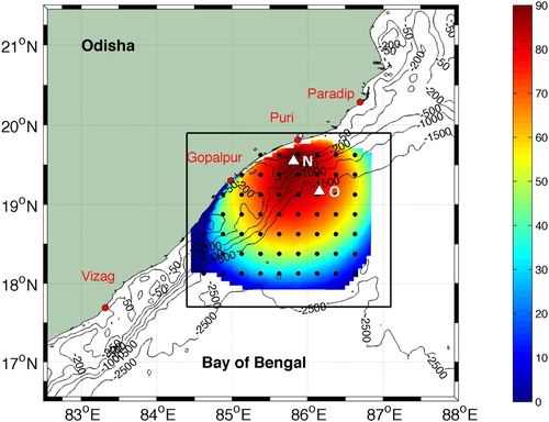
This study has been carried out using the hourly HFR (SeaSonde, 4.4 MHz) surface current data with horizontal resolution of around 6 km over a limited region (17.5–20°N, 84.5–87°E) during 2010 (Figure 1). The bandwidth and wavelength of these HFR are 25 kHz and 68 m, respectively, with maximum coverage of ∼200 km in the open ocean from coastline. The year-long data are used after quality control to validate and to find the ability to capture the broad features of the current system. It is to be noted that there is no HFR data available from May till September in this domain in 2010. Excluding these months, the data coverage in percentage is depicted in Figure 1. The utility of HFR data in capturing the well-established reversal of boundary currents (northward during February–April and southward during October–December) and associated small-scale features are first validated by comparing against altimeter-derived daily current fields in Section 4.1. Since our main objective is to extract high-frequency tidal variability and its spatial distribution, a gap-free hourly time-series is required for at least 29 days with good data coverage. Thus, based on availability from this early observational period of the Indian Operational HFR Network, we have carried out the tidal analysis using a month-long data in January 2010. Certainly, this methodology can be further extended for the other available datasets in recent year in the near future.

Figure 1. The data coverage (shaded) during 2010 in percentage (%). The dots show the grid points of the ADC data. The locations of the comparison points at near shore (N; 85.81 E, 19.55 N)) and offshore (O; 86.19 E, 19.17 N) are indicated by the triangle symbol. Black contours denote the isobaths of −50, −200, −500, −1000, −1500 and −2500 m from ETOPO2. Red dots indicate HFR stations at Puri and Gopalpur in the state of Odisha, India. Also shown are the two coastal stations (Paradip and Vizag), where the tide gauge data were collected.

3.2. Other datasets and methodology

Due to the unavailability of other surface current observations in this domain, a product of surface currents is derived (henceforth, ADC: Algorithm Derived Current) following Bonjean and Lagerloef (2002) for validation of HFR surface currents. The ADC datasets are the combination of three components of surface currents obtained from satellite products, namely (i) the wind-driven (Ekman) component from winds, (ii) the geostrophic component from SSHA and (iii) the surface buoyancy component from SST, all on daily scale. The mathematical formulation of the same is as follows.

Using complex notation, the tidal current U is given by: and , the basic equations are as follows:

ifwhere denotes the pressure, f denotes the Coriolis parameter, is the vertical derivative of pressure and is the temperature, with , and subject to the following boundary conditions: A denotes the eddy viscosity coefficient which describes the process of vertical turbulent mixing is uniform with depth. The vertical shear reaches zero at a constant scaling depth of z = −H. The acceleration due to gravity is m/s² and the characteristic density is  = 1025 kg/m³. The coefficient of thermal expansion  = 3 × 10⁻⁴ K⁻¹. The vector field represents the surface wind stress divided by , whereas and are the zonal and meridional components of .

The detailed mathematical formulation for the above methodology is described in Bonjean and Lagerloef (2002), who used this algorithm for validation of surface currents in the tropical Pacific Ocean. Note that, for this study, the hourly observations of HFR are averaged on daily scale to compare with ADC as presented in Section 4.1 later.

The Advanced Scatterometer (ASCAT) satellite winds at 0.25° ×  0.25° resolution (Bentamy et al. 2012) are used for the ADC computation. SSHA from satellite altimetry at a spatial resolution of 0.25° × 0.25° are produced by Ssalto/Duacs and distributed by Aviso, with support from Cnes, http://www.aviso.altimetry.fr/duacs/. SST datasets are obtained from the Group of High Resolution Sea Surface Temperature (GHRSST) with spatial resolution of 1/12° × 1/12° (source: ftp://podaac.jpl.nasa.gov/allData/). For the validation purpose, all three datasets have been interpolated to a uniform spatial resolution of 0.25° × 0.25° (same grid of AVISO & ASCAT); grid points are shown by black dots in Figure 1. To understand the dominant tidal constituents in this region, tide gauge observations have been used at hourly scale at Paradip and Vizag (Figure 1) which are close to HFR domain.

Since spatial coverage for the HFR data is not homogenous, an offshore location ‘O’ (86.19°E, 19.17°N) have been identified for the validation which is also close to the grid of AVISO & ASCAT (Figure 1). To analyse the tidal variability of the currents from the HFR, the longest continuous time span of a month in 2010 (January) with minimum data-gaps is selected. An additional location close to shore ‘N’ (85.81°E, 19.55°N) is also chosen for the tidal analysis. Both locations (‘O’ and ‘N’) have HFR data availability of more than 90% for the time span of 31 days in January 2010. Choosing offshore and nearshore locations help to compare the tidal characteristics for the corresponding locations. Then, a full tidal harmonic analysis has been implemented for the same time period using T_Tide toolbox (Pawlowicz et al., 2002) in order to separate out the tidal constituents at both locations and for both components independently. The same toolbox is used using the complex variable (u + iv) (Gough et al. 2010; Subeesh et al. 2013) to characterise the tidal ellipses spatially associated with semi-diurnal and shallow water tidal-driven currents.

4. Results

In this section, the variability on daily time-scale is presented first (Section 4.1) and the harmonic analysis which determine the tidal variability is presented next (Section 4.2). A comparison of the daily-averaged current field from operational HFR datasets against ADC is presented in Section 4.1.1. In addition, how the daily-averaged synoptic HFR velocity vectors might be used to describe the circulation patterns in this region is discussed in Section 4.1.2. This is followed by the harmonic analysis of hourly surface currents in Section 4.2. The shallow water constituents and the associated dynamics are separately discussed in Section 4.3.

4.1. Variability on daily scale

A comparison of the daily-averaged HFR current data is carried out against the ADC using various statistical metrics, which is then followed by an example of understanding the seasonal variability in the circulation patterns using the daily-averaged HFR data set selected for different days over different months/seasons.

4.1.1. Comparison of daily-averaged HFR velocity with ADC

The HFR datasets are usually affected by false signals from radio frequency interferences, distortions in the antennae pattern or many other environmental noises (Kohut and Glenn 2003). To evaluate the accuracy of the HFR technology, comparison has been made using the radial component as well as total currents with the in-situ observations like drifters (Ohlmann et al. 2007; Molcard et al. 2009; Shadden et al. 2009), ship-based sensors, Acoustic Doppler Current Profilers (ADCPs) (Chapman et al. 1997; Kaplan et al. 2005; Cosoli et al. 2010) and pointwise current meters (Emery et al. 2004; Paduan et al. 2006). The correlation coefficients and root mean square errors (RMSEs) have been found to be within the range 0.64–0.85 and 0.04–0.06 m/s for the drifters, respectively. For the current meters, the same parameters lay within the ranges 0.39–0.77 and 0.07–0.1 m/s, whereas in case of the ADCPs the ranges are 0.7–0.9 and 0.3–0.19 m/s, respectively. In this context, many validation studies have been performed previously using the in-situ datasets. Unfortunately, such observational datasets in the coastal regions of northwestern Bay are still not available and is a critical need.

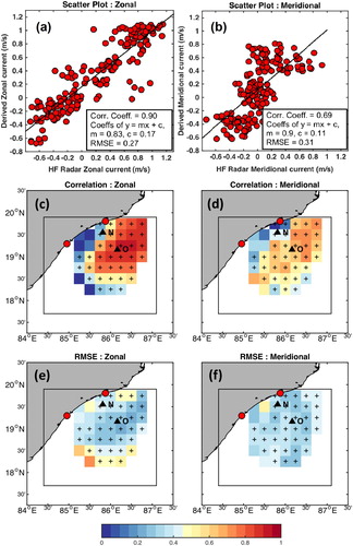
In lieu of adequate direct observations, the satellite-derived composite ADC, as discussed in the methodology section, has been adopted to compare, contrast and validate the daily-averaged HFR-derived surface current. It was earlier used for comparison of the derived products with OSCAR and in-situ datasets in the Pacific Ocean (Johnson et al. 2007) and Indian Ocean (Sikhakolli et al. 2013). In this study, validation has been done at the offshore point O, to avoid the discrepancy of satellite data very near to the coast. The comparison of the ADC and HFR-derived current for 2010 shows reasonable agreement between the two datasets in realising the seasonal variability of the circulation pattern, i.e. the northward propagating WBC during February to April and the southward propagating EICC during October and November (Figure 2). The amplitudes for the daily zonal (u) and meridional (v) components for the whole year are compared separately to obtain the correlations, the root mean square differences and the regression relation (Figure 3). The match between the two daily currents is quite well with strong correlations of 0.90 for the u-component (Figure 3(a)) and 0.69 for the v-component (Figure 3(b)), which satisfy the range as obtained from the previous studies. The respective RMSEs are 0.27 and 0.31 m/s, which are in the range of the RMSEs reported in the earlier studies described above. From the regression analysis, the best linear fit lines show the slopes with values 0.83 and 0.90 with intercepts of 0.17 and 0.11 respectively for the u- and v-components (Figure 3). In addition, the correlation maps (Figure 3(c,d)) and the RMSE maps (Figure 3(e,f)) for both of the components show lower correlations (<0.50) and higher RMSEs (∼0.40 m/s) along the coastline, whereas higher correlations (>0.85) and lower RMSEs (<0.10 m/s) in the offshore region. The ‘+’ signs indicate the points with significance level more than 95%. The significance level is calculated from the t-value obtained from their correlation coefficients and degrees of freedom (Hsin 2016; Yang et al. 2016). The poor results along the coastline are partially due to inadequacy of satellite datasets very near to the coast with significance level below 95%. Note that the correlation and RMSEs are comparatively lesser for the meridional component than those for the zonal components in the offshore regions where the results are more significant.

Figure 2. The current direction and magnitude in m/s (Sticks) for (a) HFR in upper panel and (b) ADC in lower panel at location ‘O’ for the year 2010.

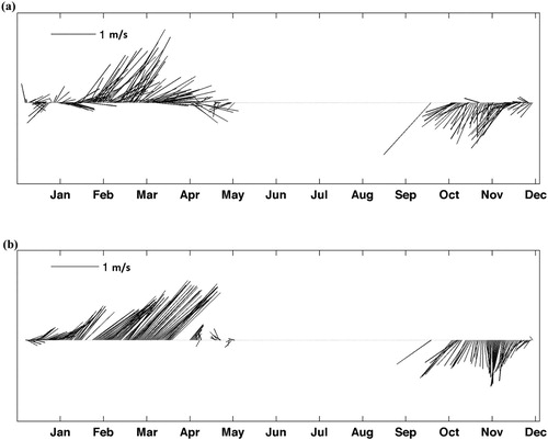
Figure 3. Comparison of daily currents from HFR and ADC (scatter dots) at O location (top), correlation maps (middle) and root mean square error (RMSE) maps (lower) during 2010 for zonal component (left) and meridional component (right). The lines through the regression plots (top panels) indicate the best fit line with value of ‘m’ for its slope and ‘c’ for the intercept. Region-wide Correlation and RMSE (in m/s) (middle and bottom panels) are colour coded to indicate their respective magnitudes. The ‘+’ signs indicate the points with significant level more than 95%.

4.1.2. Circulation variability

Next, an example of how the daily average HFR data can be used to infer circulation variability of the northwestern Bay is presented. Both HFR daily-averaged vectors are used for a selected set of days (20 January, 6 March, 16 April, 19 October, 20 November and 20 December) in 2010, overlaid with SSHA fields in Figure 4. Several circulation features are identified and described in the light of known seasonal circulation of the region.

Figure 4. HF radar-derived daily average fields of surface current in m/s (vector) with SSHA in m (shaded) for different months of 2010. Red dots indicate HFR stations at Puri and Gopalpur in the state of Odisha, India. The red line denotes 200 m isobaths.

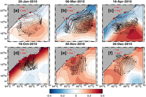
The southward flow is usually observed during the month of January, but in 2010 the surface currents are weak with magnitude of around 0.5 m/s and it is ∼100 km away from the coastline (Figure 4(a)). A small cyclonic eddy off Gopalpur coast was visible for about 15 days (9th–25th January 2010), and propagated along the coast before finally being dispersed. In the meantime, a northward flow on the western side associated with an anticyclonic eddy centred at 85.75°E, 18.50°N with radius of ∼50 km is observed, which is probably forced by the northeasterly winds (Figure 4(a)). The eddy observed along the coastline is due to the bathymetry induced continental shelf waves (Gough et al. 2010). During February–March, the southwesterly winds dominate along the coast with comparatively highly intensified WBC than in January, because the anticyclonic eddy gets intensified and dominates along the Odisha coast (Figure 4(b)). A strong meander follows the coastline along the bathymetry and reveals the presence of a clockwise eddy with positive SSHA, of which some part has been captured (Shetye et al., 1993; Somayajulu et al. 2003). The fully intensified WBC dominates the whole study region during March–April. However, during the end of March and beginning of April, the same meandering pattern continues, but an increase in current magnitude is observed from nearshore (0.5 m/s) to the offshore (1.8 m/s) (Mandal and Sil 2017). During this pre-monsoon period, the southwesterly winds dominate the whole coast, which results in increased upwelling along the coast during March–April (Figure 4(c)) (Note the near-coastal vectors are seaward and intensified). In April 2010, the currents have become slower and it is associated with anticyclonic eddy just above 18°N which is also confirmed by the satellite altimetry (Figure 4(c)). Also a cyclonic eddy is observed along the eastern part of the domain associated with the separation of the WBC along 18°N, a known feature of the springtime meandering (Figure 4(c)) (Gangopadhyay et al. 2013). Unfortunately, lack of datasets from late April to September restricts our study regarding the spring time variability.

During October–November, the northeasterly winds dominate the bay and as a result the reversal WBC (EICC) intensifies (Figure 4(d)). However, a part of the mesoscale cyclonic eddy is captured along the eastern side of the HFR coverage (Figure 4(e)) (Sil and Chakraborty 2011), which propagated southward along the highly intensified EICC during December. Another cyclonic eddy adjacent to the former is observed nearby Gopalpur coast centred at 85.10°E, 18.90°N which evolved on 1st December and persisted till 7th December, got dispersed in the open ocean while moving southwards which may be again due to the interaction with bathymetry and coastal trapped waves (Figure 4(f)) (McCreary et al. 1996). Since the circulation pattern becomes very unstable, a strong meander has developed along the southward flow with the formation of a cyclonic (anticyclonic) eddy in the southeastern (southwestern) part of the data coverage. However, the anticyclonic eddy got dispersed along the coast as the cyclonic eddy (centred at 85.85°E, 18.6°N) dominated the whole region, revealing the passage of an upwelling eddy through the same region (Figure 4(f)). Significant downwelling features are observed all along the coastline which is expected to persist, as the corresponding year is La-Nina year (Dandapat and Chakraborty 2016). A southward flow with the flow speed of about 1.2 m/s is observed along the Odisha coastline (October–December). Note that the HFR currents follow the gradients of the SSHA field well in the slope region (>200 m) indicating dominance of geostrophic regime offshore. However, the complexity of the circulation in the shelf region is apparent in the observed mismatch of the HFR currents with the underlying SSHA field. The possible factors could be a combination of the dominance of Kelvin and Continental shelf waves (Noble et al. 1987; Gough et al. 2010) on the shelf, accentuated by the increased error in the near-coastal altimeter track data.

4.2. Tidal variability on hourly scale

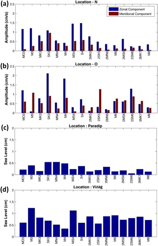
It has been now shown that the HFR currents averaged over daily period was able to match the ADC and that these fields could be used to understand the regional circulation behaviour. As mentioned in Section 1, one of our major goals in this study was to determine the shallow water constituents of the tidal variability from the hourly HFR data. However, since hourly datasets of the surface currents are not available for comparison with HFR-derived surface currents, a detailed harmonic analysis of the HFR currents was first presented to compare and contrast the presence of 28 constituents time-scales against those obtained from independent tide gauge datasets from two nearby coastal stations (Paradip and Vizag). Specifically, the diurnal (K1 and O1) and the semi-diurnal (M2, N2 and S2) constituents with significant amplitudes as observed from HFR currents (Figure 5) are compared against those obtained from tide gauge datasets (Figure 6). This comparison is discussed in Section 4.2.1. Next, the shallow water constituents (SK3, MS4, M4, S4, etc.) with significant amplitudes (from both HFR and tide gauges) are presented in Figure 7 and compared, contrasted and validated in Section 4.2.2.

Figure 5. The bars indicate the magnitude of tidally driven current (in cm/s) from HFR current data for 28 constituents at location (a) ‘N’ and (b) ‘O’ for January 2010, derived by using harmonic analysis for u-component (gray) and v-component (black).

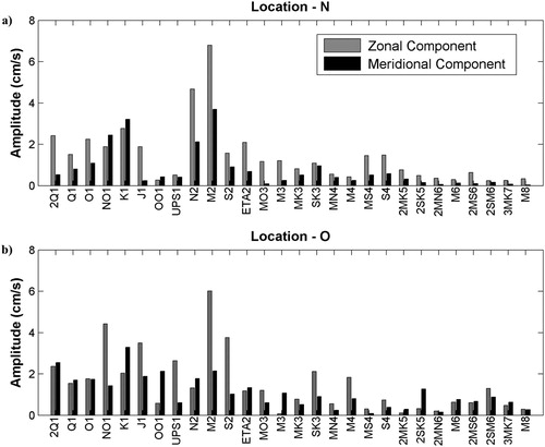
Figure 6. The bars indicate the amplitude of sea level height (in cm) from tide gauge data for 28 constituents at location (a) Paradip and (b) Vizag. Note the correspondence of relative amplitudes of the constituents with those in Figure 5, indicating the validity of HFR data enabling further high-frequency analysis.

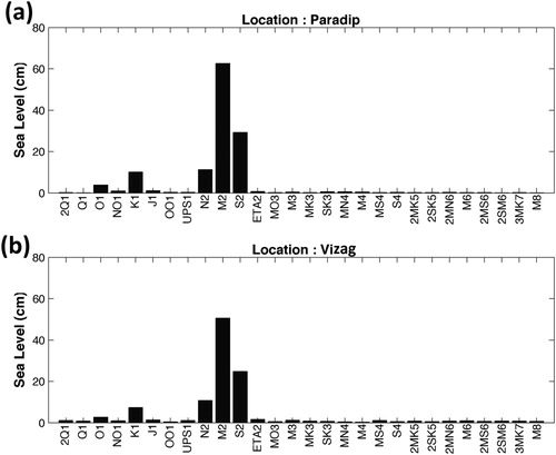
Figure 7. The amplitude of shallow water constituents for tidal-driven current (in cm/s) from HFR data at location (a) ‘N’ and (b) ‘O’; and for sea level (in cm) from tide gauge data at (c) Paradip and (d) Vizag.

4.2.1. Semi-diurnal variability comparison (M2, N2, S2)

The tidal harmonics have been analysed previously in the BoB from tide gauge observations and tidal model (Murty and Henry, 1983; Sindhu and Unnikrishnan 2013). It has been identified that the semi-diurnal signals (M2, S2 and N2) are dominant in the northwestern BoB from the previous studies. The present section represents the harmonic analysis using T_Tide toolbox in different ways. In the first part, the harmonic analysis has been performed with T_Tide toolbox individually for u- and v-components of HFR-derived ocean surface currents at both nearshore and offshore locations. The magnitude of the 28 constituents, based on the time span of the datasets (Foreman 1978a, 1978b; Pawlowicz et al. 2002), for u- and v-components at N and O location are shown in Figure 5. The semi-diurnal and diurnal constituents whose SNRs are greater than 1 are considered as significant and discussed in this section. In the second part, the same T_Tide toolbox is used with complex variable (u + iv) at the above locations to get the ellipse parameters and nature of different tidal constituents (Gough et al. 2010; Subeesh et al. 2013). The results are tabulated in Tables 1 and 2. This is extended to obtain the spatial distribution of tidal ellipses for two major tides M2 and MS4 as discussed later.

Table 1. Ellipse characteristics from harmonic tidal analysis of currents (u + iv) at the location ‘N’ for January 2010.

Tidal Constituents^a	Time period (in h.)	Major axis (cm/s)	Minor axis (cm/s)	Inclination (deg)	Phase (deg)	SNR
M2	12.25	7.16	−2.92	159.74	133.33	3.8
N2	12.40	4.71	−2.03	171.82	296.59	1.9
K1	23.56	4.02	−1.35	50.40	190.13	3.5
NO1	24.50	2.74	−1.42	121.93	183.65	2.0
2Q1	28.00	2.44	−0.38	8.75	326.30	1.2
S4	6.00	1.59	0.02	158.83	12.56	2.9
MS4	6.06	1.51	0.30	163.43	49.15	2.8
M3	8.17	1.23	−0.05	168.40	127.19	1.0
2MK5	4.56	0.83	−0.09	157.83	234.24	1.8
2MS6	4.06	0.64	0.01	170.79	24.43	1.3

Notes: Percent total variance predicted/variance original = 8.1%. Negative minor axis means clockwise circulation.

^aOnly constituents with SNRs are listed.

Table 2. Ellipse characteristics from harmonic tidal analysis of currents (u + iv) at the location ‘O’ for January 2010.

Tidal Constituents^a	Time period (in h.)	Major axis (cm/s)	Minor axis (cm/s)	Inclination (deg)	Phase (deg)	SNR
M2	12.25	6.14	1.78	11.85	168.07	4.8
NO1	24.50	4.64	0.17	17.80	190.84	3.9
J1	23.06	3.95	−0.38	152.12	0.59	2.8
S2	12.00	3.77	−0.99	4.11	289.77	1.3
2Q1	28.00	3.46	−0.26	47.28	87.04	2.8
K1	23.56	3.30	−2.04	92.95	207.57	2.9
O1	25.49	2.47	−0.14	44.62	114.14	1.5
Q1	26.52	2.22	−0.58	48.10	353.62	1.1
M4	6.13	1.97	−0.36	21.84	205.23	2.2
2SM6	4.03	1.56	−0.07	34.27	236.31	2.1
M6	4.08	0.98	0.09	50.60	201.15	1.0

Notes: Percent total variance predicted/variance original = 6.5%. Negative minor axis means clockwise circulation.

^aOnly constituents with SNRs are listed.

The M2 tidal constituent at the nearshore location has the maximum amplitude 6.79 and 4 cm/s for u- and v-components, respectively (Figure 5(a)). The second highest amplitudes are observed for N2 (4.67, 2.11 cm/s) and K1 (2.76, 3.22 cm/s) respectively for u- and v-components. The other common semi-diurnal tidal constituents at the nearshore location are S2, ETA2 and the diurnal constituents are NO1, O1 and Q1 (Figure 5a). The variance for the v-component (14.4%) is higher than that of u-component (6.8%) at the near shore location. The similar analysis for the offshore location also shows the M2 constituent to have a maximum amplitude (6.01 cm/s) for the u-component, whereas K1 (3.29 cm/s) for the v-component. At this offshore location, the other significant semi-diurnal constituents are N2 and S2 and the diurnal components are NO1, O1, Q1 and 2Q1 (Figure 5(b)) for both u- and v-components. These are mainly the derived tidal currents from the major tidal constituents, evolving as a result of interaction between the complex near-shelf bathymetry and other coastal processes (Foreman 1978a, 1978b; Pugh 1987). Tides have been also characterised in terms of form number ratio (F ratio) of tides (Defant 1961), which indicates that the tidal regime is of mixed type but predominantly semi-diurnal (F = 0.6) at both locations.

The tidal ellipses are the best way to represent the variability of the tidally driven currents and thus describing the relationship between u- and v-components (Sundar and Shetye 2005; Subeesh et al. 2013). Their study in the west coast of India reported that the maximum value of the semi-major axis is 8 cm/s on the shelf off Mumbai, whereas it is around 5 cm/s on the shelf off Goa. So, an effort has been made to study the ellipses corresponding to K1 and M2 tidal constituents in this domain of our study. At the nearshore location, the major tidal constituents M2, N2 and K1 tides are mainly clockwise in nature (negative minor axis) with semi-major axis amplitudes of values 7.16, 4.70 and 4.02 cm/s, respectively (Table 1). The other significant diurnal tidal constituents are NO1 and 2Q1 with the value of semi-major axis 2.74 and 2.43 cm/s and with clockwise orientation in nature. M2 is dominant followed by N2 agrees with the previous results (Murty and Henry 1983; Sindhu and Unnikrishnan 2013). Similarly, at the offshore location M2 is dominant with highest semi-major axis of value 6.14 cm/s but with counter-clockwise orientation. The following tidal constituent is NO1 with 4.64 cm/s semi-major axis also has counter-clockwise orientation. At this location, the other major semi-diurnal constituent is S2 and diurnal constituents are K1, O1 and Q1. The tidal properties of all significant constituents are listed in Table 2. A total tidal variance of 8.1% was observed for the nearshore location, whereas 6.5% for the offshore location (Tables 1 and 2).

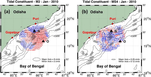
The amplitudes of the M2 tidal ellipses are relatively low and are a combination of clockwise and counter-clockwise orientations (Figure 8(a)). The patterns corresponding to M2 tidal ellipse clearly indicate a switch over of the rotational direction from clockwise along the coastal region to counter-clockwise towards the open sea. This spatial variability indicates a significant presence of the strong semi-diurnal internal tides in this region due to barotropic forcing in the cross-isobaths direction (Jithin et al. 2017). Other possible reasons are stratification and bottom friction (Bravo et al. 2013; Subeesh and Unnikrishnan 2016). The tidal ellipses change their orientations to being perpendicular to the bathymetry at depths shallower than 1500 m. This indicates that the M2-driven currents are perpendicular to the coast and get enhanced by their non-linear interaction with topography. It is to be noted that the M2 tide tends to propagate northwestward towards the head of the bay (Figure 8(a)), which can be well validated with the earlier studies (Murty and Henry 1983; Sindhu and Unnikrishnan 2013, Jithin et al. 2017).

Figure 8. (a) M2 and (b) MS4 tidal ellipses derived from harmonic analysis of HFR current data. The blue (red) ellipses mean clockwise (counter-clockwise) rotation. The black contours indicate the isobaths. Black ellipse is the reference ellipse. Red dots indicate HFR stations at Puri and Gopalpur, Odisha, India.

4.2.2. Shallow water tidal constituents (M4, S4, MS4, etc.)

The shallow water tidal constituents obtained from the tidal analysis are described in the present section for u- and v-components individually and also with complex form (u + iv), at both the nearshore and offshore locations. Only the significant shallow water constituents with SNRs greater than 1 are discussed here.

At the nearshore location, the results reveal that for the u-component, the third diurnal constituents, MO3 (resultant of M2 and O1), the fourth diurnal constituents MS4 (resultant of M2 and S2) and S4 (resultant of S2) are having amplitudes within the range 1–2 cm/s (Figure 7(a)). The tidal constituents 2MK5 and 2MS6 are having amplitudes less than 1 cm/s. For the v-component, the only significant shallow water tidal constituent observed is the third diurnal constituent SK3 (resultant of S2 and K1) with amplitude ∼1 cm/s (Figure 5(b)). At the offshore location, the most dominating and significant ones are SK3, M4 and 2SM6 with amplitudes of about 1–2 cm/s for the u-component. Whereas, for the v-component, the magnitude of shallow water constituents is comparatively less than u-component from this analysis (Figure 7(b)). The above-mentioned shallow water constituents are also observed in the tide gauge observations (Figure 7(c,d)), thus validating the time-scale content in the hourly HFR data and its applicability for further analysis to identify the shallow water constituents. It is to be noted that the amplitudes of shallow water constituents for the two tide gauges are different; possible reasons could be a mix of their different geographical positions, tidal interactions with complex bathymetry and other coastal circulation processes (Foreman 1978a, 1978b; Pugh 1987).

The analysis, combining both components as a complex variable (u + iv), indicates that at the nearshore location, the third diurnal constituents M3 and fourth diurnal MS4 and S4 with semi-major axis amplitudes about 1–2 cm/s (Table 1). Also, 2MK5 and 2MS6 are other shallow water tidal constituents having amplitudes less than 1 cm/s. At the offshore location, the M4, M6 and 2SM6 are significant with amplitudes 1.97, 0.99 and 1.56 cm/s, respectively (Table 2). It is to be noted here that, the tidal analyses of u-component and complex unit show similar results at both the locations. Generally, in a semi-diurnal tidal regime, the amplitudes corresponding to the higher order odd shallow water harmonic constituents are usually very small, which clearly satisfies the results from our analysis (Pugh 1987).

The major axes of tidal ellipses for MS4, which is compound tide of two dominating tidal constituents M2 and S2, indicate that the amplitudes are increasing in the region of steep bathymetry while propagating towards the coast. The orientations of the ellipses reveal that the maximum currents due to tides are oriented parallel to isobaths in the offshore region and perpendicular to the bathymetry (Figure 8(b)) as one nears the coast.

5. Summary and conclusions

This paper presents first results for application of the operational HFR-derived ocean current for identifying shallow water constituents through sequential and systematic validation and the tidal analysis along Odisha coast in the northwestern BoB. The validation was carried out in two distinct steps: (i) first, by comparing daily average HFR current against satellite-derived ADC and (ii) second, by comparing and contrasting time-scales of 28 tidal constituents in the HFR data against independent tide gauge data from two nearby coastal stations. A diagnostic algorithm has been designed following Bonjean and Lagerloef (2002) for estimation of the daily surface currents (ADC) combining wind-driven current, geostrophic current and buoyancy driven current, which are derived from satellite products of wind, SSHA and SST, respectively. Both the HFR-derived ocean surface currents and the ADC are analysed statistically. From the analysis, a higher correlation for the zonal component along with moderate correlation for the meridional component has been observed with less RMSE which are in the range of HFR validation in the other coastal region. The northward current during spring and its reversal in the autumn are well captured from the current pattern and it also quantified the magnitude of the current. The higher correlation and ability to identify the broad scale features gave us the confidence for higher analysis, namely spectral analysis and higher harmonic analysis.

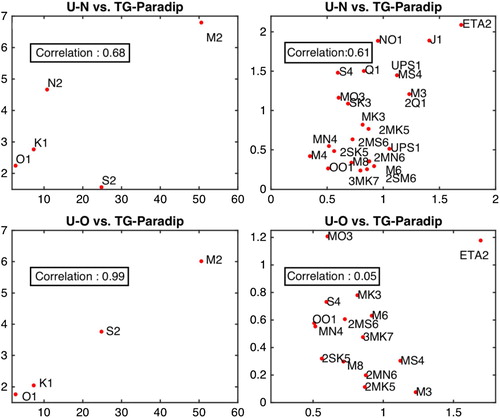
Next, a detailed harmonic analysis of the HFR currents is presented to compare and contrast the existence of 28 constituents time-scales against those obtained from independent tide gauge datasets from two nearby coastal stations (Paradip and Vizag). Tidal harmonic analyses of the individual u- and v-components and with complex form have been performed on surface currents over January 2010 when a time-series of HFR data is available with minimum gaps for a month period. The result points out that the amplitudes of the M2 and N2 tidal components are dominating both for u- and v-components at the nearshore location. At both nearshore and offshore locations, the amplitude for M2 tidal constituent for u-component is more than the v-component. But in case of K1, the amplitude is higher for v-component at both locations. Nearshore region showed greater tidal variance compared to the offshore region. A quantitative regression analysis was carried out to compare the major and minor tidal constituent amplitudes obtained from HFR surface currents and those from the tide gauge sea level data at Paradip. Since the tides are aligned in the zonal direction the tidal elevations constituents are indeed well-correlated with those of the zonal component of the HFR current (Figure 9). For the major constituents (mainly M2, K1, O1), the sea level amplitudes have larger correlation (0.99) with the zonal currents at the offshore location ‘O’ compared to location ‘N’ (0.68). For most of the minor constituents, the sea level amplitudes are significantly correlated to the zonal currents from HFR at N point (r = 0.61), while they are uncorrelated at the O point. This indicates the low-frequency tidal constituents (semi-diurnal and diurnal) of the currents match well with the sea level variations observed at the tide gauges. The fact that the correlation at ‘N’ is less than at ‘O’ implies that the shallow bathymetry plays a role on the modulating the amplitudes of the major constituents and energy might be cascading to higher frequency components. It is evident from the high significance of low-frequency constituents at both locations and the progressive increase of correlation from O to N for the high-frequency components, both major and shallow water constituents are being resolved by the HFR currents near the coast. This points to the possible utility of the HFR data for understanding near-coastal processes along the Indian Coast. Furthermore, at the nearshore location, the major tidal constituents M2, N2 and K1 tides are mainly clockwise in nature (negative minor axis) and the offshore location M2 is dominant but with counter-clockwise orientation. At the offshore location, the other identified major constituents are semi-diurnal constituent S2 and diurnal constituent K1. The higher variability for the tidal ellipses of M2 is observed in amplitude, rotational orientation, inclination and eccentricity. At the offshore location, semi-diurnal clockwise and counter-clockwise ellipses are more dominating than the diurnal (Figure 8).

Finally, besides the prominent tidal semi-diurnal and diurnal constituents, our study then identified the shallow water constituents from the harmonic analysis with u- and v-components individually and also by combining them. The significant shallow water constituents S4, MS4 and M3 (M4, 2SM6 and M6) with amplitudes of semi-major axis of about 1 to 2 cm/s are identified at nearshore (offshore) location. The distribution and orientations of the ellipses of the MS4 tides (Figure 8(b)) clearly indicate that the shallow water constituents are due to complex and non-linear tidal interaction with the bathymetry. Identifying different interaction factors (bottom bathymetric slope, bottom friction, curvature of the coastline, etc.) would be of future interest, which could be done by setting up careful and systematic numerical modelling experiments with target sensitivity studies to understand the complexity and partitioning the impacts of such forcing/interaction set ups.

Figure 9. The correlations between the major (left panel) and minor (right panel) tidal constituents (in terms of amplitude) obtained from HFR (y axis in cm/s) derived zonal component at N (top) and O (bottom) locations with tide gauge at Paradip (x axis in cm).

To conclude, it is a humble submission that the first analysis of tidal components identifiable from HFR data for the northwestern BoB has been presented, which will help develop further assimilation methodologies of HFR data on tidal-time-scales as was done for operational models for coastal waters of New York and New Jersey by Gopalakrishnan and Blumberg (2012). It is noted in passing that long-term sustenance of such HFR observational sites is critical for obtaining the barotropic tides in this region, which will also help in future numerical modelling and understanding internal tides due to prevalent regional topographic features. The earlier studies for the BoB have reproduced the basic semi-diurnal and diurnal tidal constituents quite well. To our knowledge, this is the first study in which the high-frequency components from HFR currents and the shallow water tides are also adequately resolved for this region.

Acknowledgements

The authors sincerely thank Dr. B. K. Jena and his Coastal and Environmental Engineering Group, National Institute of Ocean Technology (NIOT), Chennai for constant monitoring of the HF Radars and making the data availability efficient. The authors are grateful to anonymous reviewers and the editor for their valuable suggestions and comments. Finally, the help and infrastructural support provided by various offices of the Indian Institute of Technology Bhubaneswar (IITBBS) is also acknowledged.

Disclosure statement

No potential conflict of interest was reported by the authors.

ORCID

Samiran Mandal http://orcid.org/0000-0003-3223-1674

Sourav Sil http://orcid.org/0000-0002-6846-2071

Avijit Gangopadhyay http://orcid.org/0000-0002-7412-7325

Debadatta Swain http://orcid.org/0000-0001-6324-4107

Additional information

Funding

Authors acknowledge the financial support given by the Earth System Science Organization (ESSO) – Indian National Centre for Ocean Information Services (INCOIS), Ministry of Earth Sciences (MoES) and Science and Engineering Research Board (SERB) of Department of Science and Technology (DST), Government of India. SS and DS thank partly supports from MoES for the Bay of Bengal Coastal Observatory (BoBCO) project and Space Application Centre (SAC), Indian Space Research Organisation (ISRO). AG wishes to thank SMAST colleagues and Mid-Atlantic Regional Association Coastal Ocean Observing System (MARACOOS) support (under National Oceanic and Atmospheric Administration (NOAA) grant number NA11NOS0120038 for the implementation of the MARACOOS).

References

- Andersen OB. 1999. Shallow water tides in the northwest European shelf region from TOPEX/ POSEIDON altimetry. J Geophys Res. 104(C4):7729–7741. doi:10.1029/1998JC900112.
- Antony C, Unnikrishnan AS. 2013. Observed characteristics of tide-surge interaction along the east coast of India and the head of Bay of Bengal. Estuar Coast Shelf Sci. 131:6–11. doi:10.1016/j.ecss.2013.08.004.
- Babu MT, Sarma YVB, Murty VSN, Vethamony P. 2003. On the circulation in the Bay of Bengal during northern the spring intermonsoon (March–April 1987). Deep Sea Res II. doi:10.1016/S0967-0645(02)00609-4.
- Barrick DE, Evans MW, Weber BL. 1977. Ocean surface currents mapped by Radar. Science. 198(4313):138–144. doi:10.1126/science.198.4313.138.
- Bentamy A, Grodsky SA, Carton JA, Croizé-Fillon D, Chapron B. 2012. Matching ASCAT and QuikSCAT winds. J Geophys Res. 117. doi:10.1029/2011JC007479.
- Bravo L, Ramos M, Sobarzo M, Pizarro O, Valle-Levinson A. 2013. Barotropic and baroclinic semidiurnal tidal currents in two contrasting coastal upwelling zones of Chile. J Geophys Res Oceans. 118:1226–1238. doi:10.1002/jgrc.20128.
- Bonjean F, Lagerloef GSE. 2002. Diagnostic model and analysis of the surface currents in the tropical Pacific Ocean. J Phys Oceanogr. 32:2938–2954. doi: 10.1175/1520-0485(2002)032<2938:DMAAOT>2.0.CO;2
- Chapman RD, Graber HC. 1997. Validation of HF radar measurements. Oceanography. 10:76–79. doi: 10.5670/oceanog.1997.28
- Chapman RD, Shay LK, Graber HC, Edson JB, Karachintsev A, Trump CL, Ross DB. 1997. On the accuracy of HF radar surface current measurements: intercomparison with ship-based sensors. J Geophys Res. 102:18737–18748. doi: 10.1029/97JC00049
- Cheng X, Xie S-P, McCreary JP, Qi Y, Du Y. 2013. Intraseasonal variability of sea surface height in the Bay of Bengal. J Geophys Res Oceans. 118:816–830. doi:10.1002/jgrc.20075.
- Cosoli S, Bolzon G, Mazzoldi A. 2012. A real-time and offline quality control methodology for SeaSonde high-frequency radar currents. J Atmos Oceanic Technol. 29:1313–1328. doi:10.1175/JTECH-D-11-00217.1.
- Cosoli S, Mazzoldi A, Gačić M. 2010. Validation of surface current measurements in the Northern Adriatic Sea from high-frequency radars. J Atmos Oceanic Technol. 27:908–919. doi: 10.1175/2009JTECHO680.1
- Dandapat S, Chakraborty A. 2016. Mesoscale eddies in the Western Bay of Bengal as observed from satellite altimetry in 1993–2014: statistical characteristics, variability and three-dimensional properties. IEEE J Sel Top Appl Earth Obs Remote Sens. 9:5044–5054. doi: 10.1109/JSTARS.2016.2585179
- Defant A. 1961. Physical oceanography. Vol. 2. New York: Pergamon Press. 598 pp.
- Dey D, Sil S, Jana S, Pramanik S, Pandey PC. 2017. An assessment of TropFlux and NCEP air-sea fluxes on ROMS simulations over the Bay of Bengal region. Dynam Atmos Ocean. 80:47–61. doi: 10.1016/j.dynatmoce.2017.09.002
- Emery B, Washburn ML, Harlan JA. 2004. Evaluating radial current measurements from CODAR high-frequency radars with moored current meters. J Atmos Oceanic Technol. 21:1259–1271. doi: 10.1175/1520-0426(2004)021<1259:ERCMFC>2.0.CO;2
- Foreman MGG. 1978a. Manual for tidal heights analysis and prediction. Technical Report Pacific Marine Science Report 77–10. Patricia Bay, Sidney, BC: Institute of Ocean Sciences.
- Foreman MGG. 1978b. Manual for tidal currents analysis and prediction. Technical Report Pacific Marine Science Report 78–6. Patricia Bay, Sidney, BC: Institute of Ocean Sciences.
- Gangopadhyay A, Bharat Raj GN, Chaudhuri AH, Babu MT, Sengupta D. 2013. On the nature of meandering of the springtime western boundary current in the Bay of Bengal. Geophys Res Lett. 40:2188–2193. doi:10.1002/grl.50412.
- Gopalakrishnan G, Blumberg AF. 2012. Assimilation of HF radar-derived surface currents on tidal timescales. J Oper Oceanogr. 5:75–87. doi: 10.1080/1755876X.2012.11020133
- Gough MK, Garfield N, McPhee-Shaw E. 2010. An analysis of HF radar measured surface currents to determine tidal, wind-forced, and seasonal circulation in the Gulf of the Farallones, California, United States. J Geophys Res. 15:C04019. doi:10.1029/2009JC005644.
- He Y, Lu X, Qiu Z, Zhao J. 2004. Shallow water tidal constituents in the Bohai Sea and the Yellow Sea from a numerical adjoint model with TOPEX/ POSEIDON altimeter data. Continental Shelf Res 24(13–14):1521–1529. doi: 10.1016/j.csr.2004.05.008
- Hsin Y. 2016. Trends of the pathways and intensities of surface equatorial current system in the North Pacific Ocean. J Climate. 29:6693–6710. doi:10.1175/JCLI-D-15-0850.1.
- Jana S, Gangopadhyay A, Chakraborty A. 2015. Impact of seasonal river input on the Bay of Bengal simulation. Cont Shelf Res. 104:45–62. doi:10.1016/j.csr.2015.05.001.
- Jana S, Gangopadhyay A, Lermusiaux P, Chakraborty A, Sil S, Haley PJ. 2018. Sensitivity of the Bay of Bengal upper ocean to different winds and river input conditions. J Mar Syst.
- Jithin AK, Unnikrishnan AS, Fernando V, Subeesh MP, Fernandes R, Khalap S, Narayan S, Agarvadekar Y, Gaonkar M, Tari P, et al. 2017. Observed tidal currents on the continental shelf off the east coast of India. Cont Shelf Res. 141:51–67. doi:10.1016/j.csr.2017.04.001.
- John M, Jena BK, Sivakholundu KM. 2015. Surface current and wave measurement during cyclone Phailin by high frequency radars along the Indian coast. Curr Sci. 108(3):405–409.
- Johnson ES, Bonjean F, Lagerloef GSE, Gunn JT, Mitchum GT. 2007. Validation and error analysis of OSCAR sea surface currents. J Atmos Ocean Technol. 24:688–701. doi: 10.1175/JTECH1971.1
- Kaplan DM, Largier J, Botsford LW. 2005. HF radar observations of surface circulation off Bodega Bay (Northern California. USA). J Geophys Res. 110:322. doi:10.1029/2005J C002959 doi: 10.1029/2005JC002959
- Kim SY, Terrill E, Cornuelle B. 2007. Objectively mapping HF radar-derived surface current data using measured and idealized data covariance matrices. J Geophys Res. 112:C06021. doi:10.1029/2006JC003756.
- Kohut JT, Glenn SM. 2003. Improving HF radar surface current measurements with measured antenna beam patterns. J Atmos Ocean Technol. 20:1303–1316. doi: 10.1175/1520-0426(2003)020<1303:IHRSCM>2.0.CO;2
- Kurien P, Ikeda M, Valsala VK. 2010. Mesoscale variability along the East Coast of India in spring as revealed from satellite data and OGCM simulations. J Oceanogr. 66:273–289. doi: 10.1007/s10872-010-0024-x
- Mandal S, Sil S. 2017. Coastal currents from HF radars along Odisha coast. Ocean Dig Q Newsl Ocean Soc India. 4:4–6.
- McCreary J, Han W, Shankar D, Shetye SR. 1996. Dynamics of the East India Coastal Current: 2. Numerical Solutions. J Geophys Res. 101:13999–14010. doi:10.1029/96JC00560.
- Molcard A, Poulain PM, Forget P, Griffa A, Barbin Y, Gaggelli J, De Maistre JC, Rixen M. 2009. Comparison between VHF radar observations and data from drifter clusters in the Gulf of La Spezia (Mediterranean Sea). J Mar Syst. 78:S79–S89. doi: 10.1016/j.jmarsys.2009.01.012
- Mukhopadhyay S, Shankar D, Aparna SG, Mukherjee A. 2017. Observations of the sub-inertial, near-surface East India Coastal Current. Cont Shelf Res. 148:159–177. doi:10.1016/j.csr.2017.08.020.
- Murty TS, Henry RF. 1983. Tidal harmonics in the Bay of Bengal. J Geophys Res. 88(C10):6069–6076. doi: 10.1029/JC088iC10p06069
- Noble M, Rosenfeld LK, Smith RL, Gardner JV, Beardsley RC. 1987. Tidal currents seaward of the northern California continental shelf. J Geophys Res. 92(C2):1733–1744. doi:10.1029/JC092iC02p01733.
- Ohlmann C, White P, Washburn L, Terrill E, Emery B, Otero M. 2007. Interpretation of coastal HF radar-derived currents with high-resolution drifter data. J Atmos Ocean Technol. 24:666–680. doi: 10.1175/JTECH1998.1
- Paduan JD, Kim KC, Cook MS, Chavez FP. 2006. Calibration and validation of direction-finding high-frequency radar ocean surface current observations. IEEE J Oceanic Eng. 31(4):862–875. doi: 10.1109/JOE.2006.886195
- Paduan JD, Rosenfield LK. 1996. Remotely sensed surface currents in Montery Bay from shore-based HF radar (Coastal Ocean dynamics application radar). J Geophys Res Oceans. 118:816–830. doi:10.1002/jgrc.20075.
- Pawlowicz R, Beardsley B, Lentz S. 2002. Classical tidal harmonic analysis including error estimates in MATLAB using T_TIDE. Comput Geosci. 28(8):929–937. doi:10.1016/S0098-3004(02)00013-4.
- Prandle D. 1987. The fine-structure of nearshore tidal and residual circulations revealed by H. F. Radar surface current measurements. J Phys Oceanogr. 17:231–245. doi: 10.1175/1520-0485(1987)017<0231:TFSONT>2.0.CO;2
- Pugh DT. 1987. Tides, surges and mean sea-level, a handbook for engineers and scientists. New York: John Wiley.
- Ramp SR, Barrick DE, Ito T, Cook MS. 2008. Variability of the Kuroshio current south of Sagami Bay as observed using long-range coastal HF radars. J Geophys Res. 113:C06024. doi:10.1029/2007JC004132.
- Roarty HJ, Glenn SM, Kohut JT, Gong D, Handel E, Rivera E, Garner T, Atkinson L, Jakubiak C, Brown W, et al. 2010. Operation and application of a regional high frequency radar network in the Mid Atlantic bight. Mar Technol Soc J. 44:133–145. doi: 10.4031/MTSJ.44.6.5
- Rose L, Bhaskaran PK, Kani SP. 2015. Tidal analysis and prediction for the Gangra location. Hooghly estuary in the Bay of Bengal. Curr Sci. 109:745–758.
- Shadden SC, Lekien F, Paduan JD, Chavez FP, Marsden JE. 2009. The correlation between surface drifters and coherent structures based on high-frequency radar data in Monterey Bay. Deep Sea Res Part II. 56(3–5):161–172. doi: 10.1016/j.dsr2.2008.08.008
- Shankar D, McCreary JP, Han W, Shetye SR. 1996. Dynamics of the East India Coastal Current. 1. Analytic solutions forced by interior Ekman pumping and local alongshore winds. J Geophys Res. 101(C6):13 975–13991. doi: 10.1029/96JC00559
- Shay LK, Graber HC, Ross DB, Chapman RD. 1995. Mesoscale ocean surface current structure detected by HF radar. J Atmos Ocean Technol. 12:881–900. doi: 10.1175/1520-0426(1995)012<0881:MOSCSD>2.0.CO;2
- Shetye SR, Gouveia AD, Shenoi SSC, Sundar D, Michael GS, Nampoothiri G. 1993. The western boundary current of the seasonal subtropical gyre in the Bay of Bengal. J Geophys Res. 98:945–954. doi: 10.1029/92JC02070
- Sil S, Chakraborty A. 2011. Simulation of East India Coastal features and validation with satellite altimetry and drifter climatology. Int J Oceans Clim Syst. 2(4):279–289. doi: 10.1260/1759-3131.2.4.279
- Sil S, Chakraborty A, Basu SK, Pandey PC. 2014. Response of OceanSat II scatterometer winds in the Bay of Bengal circulation. Int J Remote Sens. 35(14):5315–5327. doi: 10.1080/01431161.2014.926423
- Sikhakolli R, Sharma R, Kumar R, Gohil BS, Sarkar A, Prasad KVSR, Basu S. 2013. Improved determination of Indian ocean surface currents using satellite data. Remote Sens Lett. 4:335–343. doi: 10.1080/2150704X.2012.730643
- Sindhu B, Unnikrishnan AS. 2013. Characteristics of tides in the Bay of Bengal. Mar Geod. 36:377–407. doi: 10.1080/01490419.2013.781088
- Sinha PC, Jain I, Bhardwaj N, Rao AD, Dube SK. 2008. Numerical modeling of tide-surge interaction along Orissa coast of India. Nat Hazards. 45:413–427. doi: 10.1007/s11069-007-9176-4
- Somayajulu YK, Murty VSN, Sarma YVB. 2003. Seasonal and inter-annual variability of surface circulation in the Bay of Bengal from TOPEX/ Poseidon altimetry. Deep Sea Res II. 50:867–880. doi:10.1016/S0967-0645(02)00610-0.
- Subeesh MP, Unnikrishnan AS, Fernando V, Agarwadekar Y, Khalap ST, Satelkar NP, Shenoi SSC. 2013. Observed tidal currents on the continental shelf off the west coast of India. Cont Shelf Res. 69:123–140. doi: 10.1016/j.csr.2013.09.008
- Subeesh MP, Unnikrishnan AS. 2016. Observed internal tides and near-inertial waves on the continental shelf and slope off Jaigarh, central west coast of India. J Mar Syst. 157:1–19. doi: 10.1016/j.jmarsys.2015.12.005
- Sundar D, Shetye SR. 2005. Tides in the Mandovi and Zuari estuaries, Goa, west coast of India. J Earth Syst Sci. 114(5):493–503. doi: 10.1007/BF02702025
- Ullman DS, Codiga DL. 2004. Seasonal variation of a coastal jet in the long Island sound outflow region based on HF radar and Doppler current observations. J Geophys Res. 109:304. doi:10.1029/2002JC001660.
- Yang H, Lohmann G, Wei W, Dima M, Ionita M, Liu J. 2016. Intensification and poleward shift of subtropical western boundary currents in a warming climate. J Geophys Res Oceans. 121:4928–4945. doi:10.1002/2015JC011513.