Copernicus Marine Service Ocean State Report

Table of Contents

Introduction — s1

Chapter 1: Essential Variables — s4

 1.1 Ocean temperature and salinity

  Sandrine Mulet, Bruno Buongiorno Nardelli, Simon Good, Andrea Pisano, Eric Greiner, Maeva Monier, Emmanuelle Autret, Lars Axell, Fredrik Boberg, Stefania Ciliberti, Marie Drévillon, Riccardo Droghei, Owen Embury, Jérome Gourrion, Jacob Høyer, Mélanie Juza, John Kennedy, Benedicte Lemieux-Dudon, Elisaveta Peneva, Rebecca Reid, Simona Simoncelli, Andrea Storto, Jonathan Tinker, Karina von Schuckmann and Sarah L. Wakelin — s5

 1.2 Sea level

  Jean-François Legeais, Karina von Schuckmann, Angelique Melet, Andrea Storto and Benoit Meyssignac — s13

 1.3 Currents

  Marie Drévillon, Jonathan Tinker, Romain Bourdallé-Badie, Eric Greiner, Hélène Etienne, Marie-Hélène Rio, Yann Drillet and Fabrice Hernandez — s16

 1.4 Sea ice

  Annette Samuelsen, Gilles Garric, Roshin P. Raj, Lars Axell, Hao Zuo, K. Andrew Peterson, Signe Aaboe, Andrea Storto, Thomas Lavergne and Lars-Anders Breivik — s20

 1.5 Ocean colour

  Shubha Sathyendranath, Silvia Pardo, Mario Benincasa, Vittorio E. Brando, Robert J.W. Brewin, Frédéric Mélin and Rosalia Santoleri — s23

 1.6 Nitrates

  Coralie Perruche, Cosimo Solidoro and Stefano Salon — s26

 1.7 Air-to-sea carbon flux

  Coralie Perruche, Cosimo Solidoro and Gianpiero Cossarini — s29

 1.8 Wind

  Ad Stoffelen, Jos de Kloe, Ana Trindade, Daphne van Zanten, Anton Verhoef and Abderahim Bentamy — s33

Chapter 2: Changes in ocean climate — s41

 2.1 Ocean heat content

  Karina von Schuckmann, Andrea Storto, Simona Simoncelli, Roshin P. Raj, Annette Samuelsen, Alvaro de Pascual Collar, Marcos Garcia Sotillo, Tanguy Szerkely, Michael Mayer, K. Andrew Peterson, Hao Zuo, Gilles Garric and Maeva Monier — s41

 2.2 Steric sea level

  Andrea Storto, Karina von Schuckmann, Jean-François Legeais, Tanguy Szerkely, K. Andrew Peterson, Hao Zuo and Gilles Garric — s45

 2.3 Mass and heat transports

  Clément Bricaud, Gilles Garric, Yann Drillet, Hao Zuo, Andrea Storto and Karina von Schuckmann — s49

 2.4 Oxygen minimum zones

  Elodie Gutknecht, Aurélien Paulmier and Coralie Perruche — s53

 2.5 Oligotrophic gyres

  Shubha Sathyendranath, Silvia Pardo and Robert J.W. Brewin — s55

 2.6 El Niño southern oscillation

  Florent Gasparin, Karina von Schuckmann, Charles Desportes, Shubha Sathyendranath, Silvia Pardo, Eric Greiner and Clotilde Dubois — s56

 2.7 Western boundary currents

  Marie Drévillon, Jean-François Legeais, Andrea Storto, K. Andrew Peterson, Hao Zuo, Marie-Hélène Rio, Yann Drillet and Eric Greiner — s60

 2.8 Atlantic Meridional Overturning Circulation

  Laura Jackson, Clotilde Dubois, Simona Masina, Andrea Storto and Hao Zuo — s65

 2.9 Changes in the North Atlantic

  Clotilde Dubois, Karina von Schuckmann, Simon Josey and Adrien Ceschin — s66

 2.10 Arctic ocean freshwater content

  Gilles Garric, Olga Hernandez, Clement Bricaud, Andrea Storto, Kenneth Andrew Peterson and Hao Zuo — s70

Chapter 3: Changes in the regional European seas — s79

 3.1 Sea level, SST and waves: extremes variability

  Begoña Pérez Gómez, Marta De Alfonso, Anna Zacharioudaki, Irene Pérez González, Enrique Álvarez Fanjul, Malte Müller, Marta Marcos, Fernando Manzano, Gerasimos Korres, Michalis Ravdas and Susanne Tamm — s79

 3.2 North Atlantic – Arctic exchanges

  Vidar Lien, Roshin P. Raj — s88

 3.3 Characterisation of Mediterranean outflow water in the Iberia-Gulf of Biscay-Ireland region

  Álvaro Pascual, Bruno Levier, Marcos Sotillo, Nathalie Verbrugge, Roland Aznar and Bernard Le Cann — s91

 3.4 Water mass formation processes in the Mediterranean sea over the past 30 years

  Simona Simoncelli, Nadia Pinardi, Claudia Fratianni, Clotilde Dubois, Giulio Notarstefano — s96

 3.5 Ventilation of the western Mediterranean deep water through the strait of Gibraltar

  Simone Sammartino, Jesús García Lafuente, Cristina Naranjo and Simona Simoncelli — s101

 3.6 Decline of the Black Sea oxygen inventory

  Arthur Capet, Luc Vandenbulcke, Marilaure Grégoire and Veselka Marinova — s103

 3.7 Baltic inflows

  Urmas Raudsepp, Jean-Francois Legeais, Jun She, Ilja Maljutenko and Simon Jandt — s106

 3.8 Eutrophication and hypoxia in the Baltic Sea

  Urmas Raudsepp, Jun She, Vittorio E. Brando, Mariliis Kõuts, Priidik Lagemaa, Michela Sammartino and Rosalia Santoleri — s110

Chapter 4: Remarkable events during 2016 — s120

 4.1 Extreme sea ice conditions

  Hao Zuo, Vidar S. Lien, Anne Britt Sandø, Gilles Garric, Clement Bricaud, K. Andrew Peterson, Andrea Storto, Steffen Tietsche and Michael Mayer — s120

 4.2 Deep convection in the Labrador Sea

  Julie Deshayes, Jérôme Gourrion, Mélanie Juza, Tanguy Szekely and Joaquín Tintore — s123

 4.3 A persisting cold and fresh anomaly in the Northern Atlantic

  Jérôme Gourrion, Julie Deshayes, Mélanie Juza, Tanguy Szekely and Joaquín Tintore — s125

 4.4 Unusual salinity pattern in the South Adriatic Sea in 2016

  Zoi Kokkini, Giulio Notarstefano, Pierre-Marie Poulain, Elena Mauri, Riccardo Gerin and Simona Simoncelli — s130

 4.5 Extremes of low sea level in the Northern Baltic Sea

  Jun She and Viktorsson Lena — s131

Chapter 5: Synthesis — s139

 5.1 Long-term changes — s139

 5.2 Anomalous changes during the year 2016 — s140

Introduction

The oceans regulate our weather and climate from global to regional scales. They absorb over 90% of accumulated heat in the climate system (IPCC 2013) and over a quarter of the anthropogenic carbon dioxide (Le Quéré et al. 2016). They provide nearly half of the world’s oxygen. Most of our rain and drinking water is ultimately regulated by the sea. The oceans provide food and energy and are an important source of the planet's biodiversity and ecosystem services. They are vital conduits for trade and transportation and many economic activities depend on them (OECD 2016). Our oceans are, however, under threat due to climate change and other human induced activities and it is vital to develop much better, sustainable and science-based reporting and management approaches (UN 2017). Better management of our oceans requires long-term, continuous and state-of-the art monitoring of the oceans from physics to ecosystems and global to local scales.

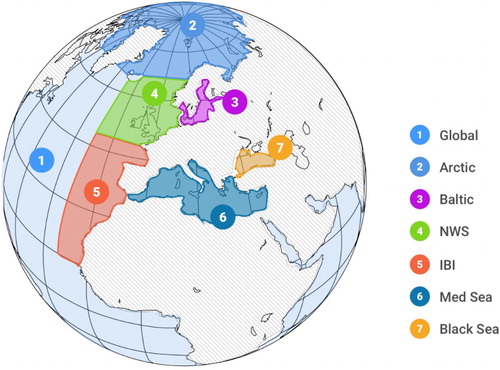
The Copernicus Marine Environment Monitoring Service (CMEMS) has been set up to address these challenges at European level. Mercator Ocean was tasked in 2014 by the European Union under a delegation agreement to implement the operational phase of the service from 2015 to 2021 (CMEMS 2014). The CMEMS now provides regular and systematic reference information on the physical state, variability and dynamics of the ocean, ice and marine ecosystems for the global ocean and the European regional seas (Figure 0.1; CMEMS 2016). This capacity encompasses the description of the current situation (analysis), the prediction of the situation 10 days ahead (forecast), and the provision of consistent retrospective data records for recent years (reprocessing and reanalysis). CMEMS provides a sustainable response to European user needs in four areas of benefits: (i) maritime safety, (ii) marine resources, (iii) coastal and marine environment and (iv) weather, seasonal forecast and climate.

Figure 0.1. CMEMS geographical areas on the map are for: 1 – Global Ocean; 2 – Arctic Ocean from 62°N to North Pole; 3 – Baltic Sea, which includes the whole Baltic Sea including Kattegat at 57.5°N from 10.5°E to 12.0°E; 4 – European North-West Shelf Sea, which includes part of the North East Atlantic Ocean from 48°N to 62°N and from 20°W to 13°E. The border with the Baltic Sea is situated in the Kattegat Strait at 57.5°N from 10.5°E.to 12.0°E; 5 – Iberia-Biscay-Ireland Regional Seas, which includes part of the North East Atlantic Ocean from 26 to 48°N and 20°W to the coast. The border with the Mediterranean Sea is situated in the Gibraltar Strait at 5.61°W; 6 – Mediterranean Sea, which includes the whole Mediterranean Sea until the Gibraltar Strait at 5.61°W and the Dardanelles Strait; 7 – Black Sea, which includes the whole Black Sea until the Bosporus Strait.

All CMEMS products are highly dependent on satellite and in-situ observations that are used to develop high level data products, validate models and constrain them through data assimilation. The development of the Copernicus Sentinel missions has already had a major impact on CMEMS and this will increase as it is fully developed (see Le Traon et al. 2017). Sea ice products and services have been strongly improved thanks to the Sentinel-1 A&B constellation. Altimeter data from Sentinel-3 improved high resolution ocean current forecasts. Ocean colour and Sea Surface Temperature (SST) from Sentinel-3 are now being tested and will very soon improve the quality of CMEMS ocean colour and SST products. Sentinel-2 is not yet integrated in CMEMS products but has already demonstrated a high potential for coastal zone monitoring. In-situ observations also play a critical role for CMEMS. They complement satellite observations by providing high quality measurements of the ocean interior. The Argo array of profiling floats has, in particular, had a major impact on the quality of CMEMS global and regional ocean reanalyses, analyses and forecasts (e.g. Turpin et al. 2016; Le Traon et al. 2017).

The development of annual ocean state reports by CMEMS is one of the priority tasks given by the EU Delegation Agreement for CMEMS implementation (CMEMS 2014). CMEMS Ocean State Reports rely on the unique capability and expertise that CMEMS gathers in Europe to monitor, assess and report on past and present marine environmental conditions (physics and biogeochemistry) and to analyse and interpret changes and trends in the marine environment. CMEMS data and products allow comprehensive monitoring of the oceans. CMEMS Ocean State Reports and associated Ocean Monitoring Indicators go one step further. They transform raw data to information and knowledge by developing science-based assessments of the state and health of our oceans and seas. They contribute to the work of European and international agencies or organisations in charge of environmental and climate monitoring, policy and their decision-makers with the additional aim of increasing general public awareness about the status of, and changes in, the marine environment. This is essential to contribute to EU policies (a major target of the Copernicus programme) and support member states in their assessment obligations. The Ocean State Report activity had been launched through the publication of the first issue (von Schuckmann et al. 2016).

The reporting is focused on the seven Copernicus Marine Service regions, i.e. the global ocean, the Arctic, the North-West Shelf, the Iberia-Biscay-Ireland, the Baltic Sea, the Mediterranean Sea and the Black Sea (Fig. 0.1). The second issue provides a view on changes in the marine environment over the period 1993–2016 and is strengthened by increased collaboration of European marine experts. Additionally, an innovative and new uncertainty assessment based on a so-called multi-product-approach is used for the reporting activity. Several Essential Variables and other large scale ocean indicators have been analysed based on ensemble means of different independent global and regional, as well as observation and reanalysis based products of the CMEMS. Uncertainties are then assessed through the spread of the different products used. They are expressed as an ‘ensemble spread’ for time series, or through the ‘signal-to-noise ratio’ (i.e. the ensemble mean over the ensemble spread) for horizontal or vertical fields. For the latter, different results show regions in which the signal exceeds the noise, i.e. when the ensemble indicates that this signature is observed in all products and can be thus classified as ‘reliable’.

A new fundamental product for the ‘multi-product-approach’ is the Global Reanalysis Ensemble Product (GREP). It contains homogeneous 3D gridded descriptions of the state of the ocean from four numerical ocean models constrained with satellite and in situ observations, forced with homogeneous atmospheric reanalysis. The monthly ensemble mean, standard deviation and individual members are distributed on the same 1 × 1° grid. Higher resolution will be available in 2018. In-depth information on the products and quality can be found on the CMEMS website.

The Ocean State Report is predominantly based on CMEMS products, and an overview on all products can be found on the web portal (http://marine.copernicus.eu/wp-content/uploads/catalogue-cmems.pdf). Some additional products have been used, such as from the Copernicus Climate Change Service, and their source is indicated in the corresponding sections, respectively. The CMEMS includes both satellite and in-situ high level products prepared by Thematic Assembly Centres (TACs) – the so-called reprocessed products – and modelling and data assimilation products prepared by Monitoring and Forecasting Centres (MFCs) – the so-called reanalysis products. CMEMS products are based on state-of-the-art data processing and modelling techniques. Products are described in Product User Manuals (PUMs).

Internationally recognised verification and validation procedures are used to assess product quality (e.g. Hernandez et al. 2015). They are continuously updated by MFCs and TACs and the overall quality of each product is monitored through regular review and routine operational verification (http://marine.copernicus.eu/services-portfolio/validation-statistics/). Quality Information Documents (QUIDs) detail these validation procedures and provide an estimate on the product accuracy and reliability. The PUMs and QuIDs are available for each CMEMS product and can be downloaded from the CMEMS online portal (http://marine.copernicus.eu/). Within this report, all CMEMS products used are linked to their product name, and provided with download links to corresponding QUID and PUM documents.

Like the first issue, the second issue consists of four principal chapters. The first chapter discusses a selection of Essential Ocean/Climate Variables. Chapter 2 further deepens this reporting with an analysis on changes in ocean climate. Chapter 3 is focused on characteristic changes in the European regional seas. These three chapters provide a monitoring and an assessment of the state, variability and change of our oceans and seas during the period 1993–2016. All anomalies are evaluated relative to the reference period 1993–2014. For some parameters, this period is somewhat shorter due to data availability issues (e.g. chlorophyll from remote sensing started in 1998). The last chapter has a specific focus on anomalous changes during 2016. A short introduction is given for all chapters. A fundamental part of the CMEMS Ocean State Report concept relies on the aim to deliver a synthesised view on selected topics and to avoid lengthy description and scientific review, and existing topic scientific review assessments have been cited whenever available. Building on the first issue of the Ocean State Report (von Schuckmann et al. 2016), the second Ocean State Report extends and deepens its analysis with the introduction of:

• The addition of four Essential Variables – sea surface salinity, nutrients, carbon flux and surface wind – in chapter one.

• The introduction of seven new topics describing changes in ocean climate, namely: steric sea level, oxygen minimum zones, oligotrophic gyres, El Niño Southern Oscillation, western boundary currents, changes in the North Atlantic area and ocean freshwater content.

• Introduction of eight ocean monitoring indicators for reporting in European regional seas.

• Reporting on specific events from 2016.

• Increased collaboration of European institutions through the addition of scientific experts.

• Introduction of new and innovative multi-product approach and related uncertainty discussions (see description above).

Chapter 1 – Essential variables

Essential Ocean Variables and Essential Climate Variables are physical, chemical or biological variables that characterise the oceans and climate. Monitoring of the Essential Variables is required to support the work of the United Nations Framework Convention on Climate Change, the Intergovernmental Panel on Climate Change (IPCC) and many marine industries and services. This concept has been broadly adopted in science and policy circles (IFSOO 2012). The objective of this chapter is to establish a state-of-the-art and scientifically sound evaluation of Essential Variable monitoring. Thus, the role of this chapter of the Ocean State Report is to continually assess and update a set of Essential Variables based on the CMEMS (and other, e.g. C3S) products each year. Depending on their availability (production and assessment), new variables are also added each year to this chapter. In this second issue of the Ocean State Report, changes over the period 1993–2016 are discussed, and an additional focus on changes during the year 2016 is delivered. Eleven different Essential Variables (four of them merged into one single section) are analysed, including four that were not discussed in the first report, i.e. sea surface salinity, nutrients, air-to-sea CO₂ flux and surface wind.

The monitoring of sea surface temperature (Section 1.1) provides insight into the flow of heat into and out of the ocean, into modes of variability at the ocean–atmosphere interface, and can be used to identify features in the ocean such as fronts and upwelling. Knowledge of its evolution is also required for applications such as ocean and weather prediction, and for climate change monitoring.

Subsurface temperature (Section 1.1) is a key Essential Ocean Variable from which the ocean heat storage (see Section 2.2) and heat transport (see Section 2.3) can be deduced. Large-scale temperature variations in the upper layers are mainly related to the heat exchange with the atmosphere and surrounding oceanic regions, while the deeper ocean temperature in the main thermocline and below varies due to many dynamical forcing mechanisms, including climate change (e.g. Forget and Wunsch 2007; Roemmich et al. 2015; Riser et al. 2016).

Sea surface salinity (Section 1.1) monitoring is crucial to evaluate changes in the global water cycle, ocean dynamics, and weather and climate (e.g. Yu et al. 2017; Durack et al. 2016; Trenberth et al. 2011). In particular, changes in sea surface salinity are closely linked to local imbalances between evaporation and precipitation, to continental runoff and to sea-ice changes. Resulting net freshwater fluxes are mediated by ocean advection and mixing and clearly feedback into water mass formation and thermohaline circulation changes.

Monitoring changes of subsurface salinity (Section 1.1) is essential, in particular, due to its link to changes in the hydrological cycle of the Earth (Curry et al. 2003; Durack et al. 2016); their essential role for changes in ocean dynamics (O’Kane et al. 2016) such as water masses formation (Kuhlbrodt et al. 2007), regional halosteric sea level change (Durack et al. 2014; Llovel and Lee 2015) and salt/freshwater transport (Vargas-Hernandez et al. 2015); and their impact on marine biodiversity (Lenoir et al. 2011).

Mean sea level (Section 1.2) rise has a direct impact on coastal areas and is a crucial index of climate change since it reflects both ocean warming and the effect of ice melt (e.g. IPCC 2013; Dieng et al. 2017).

Ocean currents (Section 1.3) transport heat, freshwater, plankton, fish, heat, momentum, oxygen and carbon dioxide and are thus a significant component of the global biogeochemical, energy and hydrological cycles. Knowledge of ocean currents is also important for marine operations involving navigation, search and rescue at sea, and the dispersal of pollutants. The ocean has an interconnected current, or circulation, system powered by winds, solar energy and water density differences, and steered by the Earth’s rotation and by tides, waves and bathymetry. Surface currents experience intrinsic oceanic interannual variability (Penduff et al. 2011; Sérazin et al. 2015); they may respond to air–sea large-scale variability patterns at interannual scale such as the North Atlantic Oscillation (Frankignoul et al. 2001), ENSO (see Section 2.6) and may undergo changes due to global warming (e.g. Yang et al. 2016; Armour et al. 2016). Deep ocean currents are density-driven and contribute to the Meridional Overturning Circulation (see Section 2.8).

Changes in sea-ice extent and volume (Section 1.4) are important for several aspects of ocean and climate monitoring, as well as for safe marine operation in and close to ice-covered regions. Sea ice is an integrated part of the climate system through its effect on surface albedo and heat and momentum flux between the ocean and the atmosphere. Sea-ice thickness, being a crucial parameter for sea-ice volume, is important for the freshwater content and cycle in the Arctic (Carmack et al. 2016), and also has an impact on the ice drift speed. Sea-ice thickness affects the opening of leads and biological production below the sea ice (Assmy et al. 2017; Horvat et al. 2017).

Ocean colour and phytoplankton (Section 1.5) are recognised as Essential Climate Variables because of the role of phytoplankton in the ocean carbon cycle; their role as the primary producers of the pelagic ocean, responsible for producing some 50 gigatons of carbon per year globally through photosynthesis; their influence on the rate of penetration of solar radiation in the ocean, through modification of the light attenuation coefficient by their absorption and scattering of light underwater; and their place at the base of the entire marine food web.

Inorganic nutrients (Section 1.6) are key components of the oceanic biogeochemical cycles. They are assimilated by autotrophic organisms to build living organic matter, moved to detritus component when living matters die, and eventually recycled back to dissolved inorganic forms at the end of the cycle. Nitrate is one of the main macro-nutrients (Sarmiento and Gruber 2006) limiting the growth of phytoplankton (primary production), which is why it has been defined as an Essential Ocean Variable.

The carbon flux between the atmosphere and ocean (Section 1.7) is an essential parameter for both the climate and the ocean systems. Superimposed on natural long-term changes (Lüthi et al. 2008), the Earth has experienced a rapid and unprecedented anthropogenic increase of atmospheric CO₂ concentrations since the beginning of the industrial era (IPCC 2013). On the one hand, the uptake of 26% of the atmospheric CO₂ by the ocean (Le Quéré et al. 2016) is buffering the impacts of anthropogenic CO₂ emissions in the atmosphere, but on the other hand, this increase of oceanic CO₂ is the main driver of contemporary ocean acidification.

Wind (Section 1.8) is the dynamical state variable of the atmosphere, and it varies significantly on time scales ranging from the meteorological scale (minutes, hours) to the climatic time scale (decades, centuries). Wind stress forces ocean dynamics, triggers mixing of water and evaporates water, while, on the other hand, the water surface triggers moist convection in the atmosphere and thus plays a role to redistribute its momentum, humidity and heat (e.g. Sprintall et al. 2014). Scatterometers are used to monitor surface winds and determine ocean forcing over recent decades.

All products used in the following sections are referenced with numbers linked to more information in corresponding product tables at the top of each section. A more detailed description on product use and methods is highlighted in the overall introduction of this report.

1.1. Ocean temperature and salinity

Leading authors: Sandrine Mulet, Bruno Buongiorno Nardelli, Simon Good, Andrea Pisano, Eric Greiner, Maeva Monier

Contributing authors: Emmanuelle Autret, Lars Axell, Fredrik Boberg, Stefania Ciliberti, Marie Drévillon, Riccardo Droghei, Owen Embury, Jérome Gourrion, Jacob Høyer, Mélanie Juza, John Kennedy, Benedicte Lemieux-Dudon, Elisaveta Peneva, Rebecca Reid, Simona Simoncelli, Andrea Storto, Jonathan Tinker, Karina von Schuckmann, Sarah L. Wakelin.

Statement of outcome: Results confirm that sea surface and subsurface temperatures have been increasing during the past two decades over the globe. The European sea surface experienced an overall warming over the period 1993–2016, enhanced surface and subsurface salinity in the Mediterranean, and large-scale freshening in the North-West Shelf area. During 2016, the global and European sea surface waters showed strong overall warm and salty conditions, except for the North Atlantic – including the North-West Shelf – and the North Pacific. In addition, positive salinity anomalies are recorded in 2016 close to the major rivers, denoting significant discharge reductions.

Products used: see Table 1.1.1.

Ocean temperature and salinity are fundamental parameters for ocean state monitoring as they trigger sea water density variations, and can thus impact ocean circulation. Historically, 3-D ocean temperature and salinity monitoring were limited by extremely irregular and sparse observational sampling (e.g. Abraham et al. 2013). This clearly hindered an accurate retrieval of the ocean state and dynamics and the assessment of interannual to decadal scale trends and associated spatial patterns even through model reanalyses (e.g. Sivareddy et al. 2017, Boyer et al., 2016). Conversely, sea surface temperature has started to be measured regularly from since the launch of the first 5-channel Advanced Very High Resolution Radiometer in late 1981, providing relatively accurate daily estimates with global coverage (Robinson, 2004). Also, since the beginning of the Argo era, the database from in situ observing platforms has rapidly grown (e.g. Riser et al. 2016). In the framework of CMEMS, in situ and remote sensing hydrographic data are combined to monitor the surface and subsurface fields through both purely observational approaches and data assimilation in numerical circulation models. Still, given the input data sparsity and the variability associated with the different algorithms used, providing reliable uncertainty information about the individual retrievals and derived metrics remains a challenge.

Here, the approach used in the first CMEMS Ocean State Report is extended to include data from 2016, as well as regional observations (product references 1.1.3 to 1.1.7) and regional reanalyses (products references 1.1.10 to 1.1.14) for the European Seas. In addition, an assessment of the level of confidence is provided for the global scale sea surface salinity and subsurface hydrographic anomalies and trends. An observation-based product (reference 1.1.8) and an ensemble of model reanalyses (product reference 1.1.9) produced by CMEMS have been used to estimate a signal-to-noise ratio (defined as the ratio between the ensemble mean anomaly/trend and the ensemble anomaly/trend spread) allowing identification of consistent signals among the different products. This signal-to-noise approach is not used for sea surface temperature analyses that are based on one product to compute 1993–2007 climatological mean (product reference 1.1.2) and on another one to compute 2016 anomalies (product reference 1.1.1). For global and regional surface salinity, regional surface temperature and global and regional subsurface hydrographic fields, the reference climatology is computed over the 1993–2014 time period, while for the global sea surface temperature it is estimated over the 1993–2007 time period.

1.1.1. Change in global ocean hydrography

1.1.1.1. Temperature

The global sea surface temperature warmed over the period 1993–2015 at a rate of 0.016 ± 0.002°C/year (Roquet et al. 2016). In accordance with this trend, the global sea surface temperature showed warming during the year 2016 (Figure 1.1.1(a)). Anomalous cold conditions, however, prevailed in the North Atlantic (a persistent feature since 2014, see Sections 2.9 and 4.3), and parts of the Southern Ocean. Compared to 2015 (Roquet et al. 2016), the positive anomalies in the eastern side of the tropical Pacific Ocean are weaker, reflecting a change in El Niño Southern Oscillation conditions (see Section 2.6). The trade wind intensification in the period 1993–2011 led to a cooling of the eastern Pacific (England et al. 2014). The weakening of the trade winds since 2014, associated with the strong 2015 El Niño, is responsible for the pause in the eastern Pacific cooling. The pattern of negative anomalies in the north-central Pacific and positive anomalies off the west coast of America is consistent with the shift in 2014 to the positive phase of the Pacific Decadal Oscillation.

Figure 1.1.1. 2016 Temperature anomaly. (a) 2016 Annual mean surface temperature (product 1.1.1) anomalies relative to the 1993–2007 climatology (product 1.1.2). (b) Depth/latitude sections of zonally averaged subsurface temperature anomalies in 2016 relative to the climatological period 1993–2014 (product 1.1.8). Hatching lines mask regions where the signal-to-noise ratio is less than two (the signal-to-noise ratio is computed from the multi-observations product 1.1.8 and the four reanalyses from product 1.1.9).

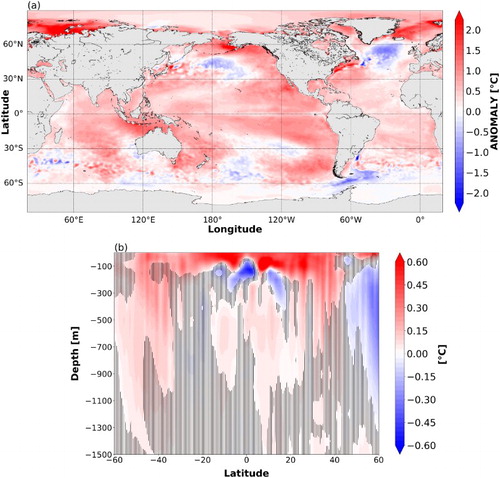
The surface warming can be felt down to 200 m in the tropics (Figure 1.1.1(b)). In the three Southern Ocean basins, the 2016 subsurface temperature shows a significant warm anomaly of around 0.3°C down to 800 m. In the northern hemisphere north of 50°N (and less than 60°N) values of −0.4°C below the mean climatology (1993–2014) occur in the upper 1000 m depth, and are linked to the cold conditions reported in the subpolar Atlantic for approximately the last 3 years (see Sections 2.9 and 4.3). In 2016, this anomaly is less pronounced at the near-surface layer compared to 2015, which appears to be linked to an earlier onset of the summer stratification in 2016 (in June 2016 compared to an onset in July 2015, not shown).

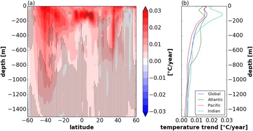
The warm temperature conditions during 2016 at the sea surface are consistent with the subsurface temperature trend over the 1993–2016 period (Figure 1.1.2). Overall warming can be observed from the surface layers down to more than 400 m depth, with the strongest subsurface warming signatures in the Indian and Atlantic Ocean (Figure 1.1.2(b)). Exceptions of this warming are manifested in the subpolar regions of both hemispheres (Figure 1.1.2(a)), which for the northern hemisphere is linked to interannual to decadal scale oceanic variations (Guinehut et al. 2016; see also Section 2.9). These results are consistent with the evaluation of ocean heat content (see Section 2.1).

Figure 1.1.2. Temperature trend. (a) Depth/latitude section of zonally averaged subsurface temperature trends (product 1.1.8) during the period 1993–2016 (in °C/year). Hatching lines mask regions where the signal-to-noise ratio is less than two (the signal-to-noise ratio is computed from the multi-observations product 1.1.8 and the four reanalyses from product 1.1.9). (b) Profiles of the subsurface temperature trends (product 1.1.8) averaged globally and by basin.

1.1.1.2. Salinity

Significant changes of sea surface salinity in 2016 occur predominantly in the Pacific and the Atlantic Ocean and in areas affected by major river runoffs (Figure 1.1.3(a)). The central Pacific is dominated by fresh conditions. This, and the increasing salinity close to Central America, is typically observed in correspondence with the displacement of the atmospheric pressure centres during the reversal of the strong 2015 El Niño to the weak 2016 La Niña (see Section 2.6, Paek et al. 2017). The positive anomalies south of the South Pacific Convergence Zone and west of the Philippines match with surface warm anomalies (Figure 1.1.3(a)). Sea surface salinity values above the mean reference (1993–2014) are observed close to the major river plumes of Amazon-Orinoco, Rio de la Plata, Mississippi, Niger, Congo, Indus and Ganges and all along the East US coast, while negative anomalies can be seen close to Yangtze (Figure 1.1.3(a)). These variations are potentially linked to the positive Pacific Decadal Oscillation since 2014 and the strong 2015 mixed El Niño conditions (e.g. Dettinger and Diaz 2000; Dai et al. 2009; Ward et al. 2010, 2014a, 2014b), though individual river basins have been shown to respond quite differently to the different phases of El Niño (see Liang et al. 2016).

Figure 1.1.3. 2016 Salinity anomaly. (a) 2016 Surface salinity anomaly relative to the 1993–2014 climatology (ensemble mean of product references 1.1.8 and 1.1.9), in practical salinity anomalies [no unit]. (b) Depth/latitude sections of zonally averaged subsurface practical salinity anomalies [no unit] in 2016 relative to the climatological period 1993–2014 (product references 1.1.8). Hatching lines mask regions where the signal-to-noise ratio is less than two. The signal-to-noise ratio in (a) is computed from the multi-observations product 1.1.8 and the 4 reanalyses from product 1.1.9 while in (b) it is computed from the multi-observations product 1.1.8 and three reanalyses from product 1.1.9: GLORYS2V4, C-GLORS05 and GloSea5).

Global subsurface salinity changes in 2016 prevail in the upper 200 m depth layers (Figure 1.1.3(b)). The tropical and subpolar regions indicate anomalous fresh hydrographic conditions. Changes in the tropical regions are triggered by variations in the Pacific Ocean and the 2015 El Niño. Fresh conditions observed at the surface in the subpolar North Atlantic extend down to more than 800 m depth (Figure 1.1.3(b)). Salty anomalies dominate the zonal average 2016 salinity anomaly in the sub-tropical regions in both hemispheres (Figure 1.1.3(b)), linked to corresponding changes in the west of the Pacific and the Atlantic (same pattern as in Figure 1.1.3(a)).

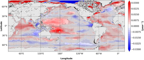
The surface salinity trend over the period 1993–2016 shows enhanced values in the western Pacific warm pool areas in both hemispheres (Figure 1.1.4). A positive trend is manifested in the North Atlantic western boundary current regime (Figure 1.1.4) and is consistent with the positive salinity anomaly in the same area during 2016 (Figure 1.1.3(a)). Significant freshening over the past two decades is restricted to the subpolar North Atlantic, which is an area dominated by interannual to decadal variations of the surface and subsurface ocean hydrographic field (see Section 4.3). This freshening is also seen clearly in the results for the changes during the year 2016. The large spread in estimated ensemble slopes, however, requires a cautious interpretation of these results. At the surface, differences are found with respect to longer term discharge trends for South and North American rivers (Milliman et al. 2008), and to the large-scale patterns associated with the intensification of the global water cycle over longer periods (Durack 2015). Indeed, the different CMEMS sea surface salinity products reach agreement on the response to shorter interannual/decadal scale processes, consistently with the relatively limited time period considered.

Figure 1.1.4. 1993–2016 Decadal trend (per year) of surface salinity (ensemble mean of product references 1.1.8 and 1.1.9). Hatching lines mask regions where the signal-to-noise ratio is less than two. The signal-to-noise ratio is computed from the multi-observations product 1.1.8 and the four reanalyses from product 1.1.9.

1.1.2. European regional seas

1.1.2.1. Temperature

Between 1993 and 2016, surface areas of all the European seas show large trends, which range from 0.030 ± 0.007°C/year in the Baltic Sea up to 0.075 ± 0.008°C/year in the Black Sea. This warming is also seen at depth but is superimposed by strong interannual variability (Figure 1.1.5). In the Baltic Sea, subsurface temperatures experience particularly strong variations at interannual time scales (Figure 1.1.5(c)), starting with several cold events at the beginning of the period, followed by relatively warm conditions during the second half of the period, in particular during the years 2014–2016.

Figure 1.1.5. Temperature time series: Top: Time series of monthly mean (thin line) and 12-month-filtered (thick line) sea surface temperature anomalies relative to 1993–2014 in the European Seas (product references 1.1.3 to 1.1.7). The sea surface temperature trend together with the 95% confidence interval (°C/year) are indicated. Bottom: Depth/time sections of subsurface temperature anomalies averaged over the European Seas during the period 1993–2016 and relative to the climatological period 1993–2014 (product references 1.1.10 to 1.1.14). The sea surface temperature trend was estimated by applying the X-11 seasonal adjustment procedure (e.g. Pezzulli et al. 2005 and references therein) and Sen’s method (Sen 1968).

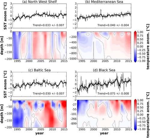
Superimposed on the surface temperature warming trend in the Black Sea (Figure 1.1.5(d)), surface and subsurface (<100 m depth) temperatures exhibit strong interannual variability (the standard deviation of the anomalies is 0.96°C), possibly linked to non-uniform and competing atmospheric forcing across the Black Sea, influenced by the cold Siberian anticyclone (North–North East) and by the milder Mediterranean weather system (South–South-West, Shapiro et al. 2010). The Mediterranean Sea (Figure 1.1.5(b)) shows basin-wide sea surface temperature warming at a rate of 0.040 ± 0.004°C/year over the period 1993–2016. This warming reaches down to deeper layers (∼600 m) but it is superimposed to interannual variability in the upper 200 m depth.

For the North-West Shelf (Figure 1.1.5(a)), the estimated trend is 0.033 ± 0.007°C/year. As in the Mediterranean Sea, the subsurface temperatures in the North-West Shelf area in the upper 200 m depth are dominated by interannual changes and mask any subsurface warming signal in this domain. This result is consistent with the evaluation of regional heat content changes (see Section 2.1).

In the Baltic Sea, the Black Sea and the Mediterranean Sea, warm sea surface temperatures are reported during the year 2016, reaching down to layers of more than 100 m depth (Figure 1.1.6). In the Baltic and Black Seas for example, anomalies exceed values of 0.5°C at the surface and in the thermocline (Figure 1.1.6(a)). The Baltic recorded anomalies even above 1°C. An abrupt surface temperature decrease at the end of 2016 is seen in the Black Sea area, probably associated with persistent negative regional land near-surface air temperature anomalies (Figure 1.1.5(d), e.g. Kennedy et al. 2017).

Figure 1.1.6. 2016 Temperature anomaly. (a) Temperature anomaly profiles in 2016 in the Baltic Sea, the North-West Shelf, the Mediterranean Sea and the Black Sea (product references 1.1.10 to 1.1.14). (b) Annual surface temperature anomalies in 2016 relative to 1993–2014 climatology in the European Seas (product references 1.1.3 to 1.1.7).

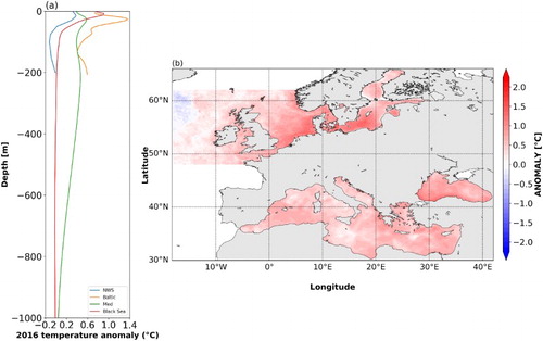
The 2016 Mediterranean Sea temperature anomaly amounts to 0.518 ± 0.001°C, slightly less than that reported for the year 2015 (0.545 ± 0.001°C, Figure 1.1.5(b)). This decrease in surface temperature has mainly occurred in the central Mediterranean Sea, i.e. the Tyrrhenian and Adriatic Seas (Figure 1.1.6(b)). This is in agreement with near-surface air temperature anomalies that were relatively low in 2016 over central and Eastern Europe (Kennedy et al. 2017). By the way, the lower 2016 anomaly with respect to 2015 also confirms 2015 as the second most exceptionally warm year after 2003 (Roquet et al. 2016).

During 2016, the impacts of the cold anomaly in the North Atlantic (see above and Sections 2.9 and 4.3) can be seen on the western North-West Shelf sea surface temperature (Figure 1.1.6(b)) and subsurface temperature, the latter reaching a negative anomaly of −0.15°C at 100 m depth (Figure 1.1.6(a)).

1.1.2.2. Salinity

An increased ocean salinity over the past 24 years is reported in the entire Mediterranean Sea from the sea surface down to more than 200 m depth (Figure 1.1.7(a,c)). A particularly strong salinity increase in the northern Ionian Sea is associated with the northern Ionian currents reversal in 1997 and a successive prevailing cyclonic circulation pattern (see also Section 3.3).

Figure 1.1.7. Salinity trend and time series. (a) 1993–2016 Decadal sea surface salinity trend (per year) in European Seas (product references 1.1.10 to 1.1.14). (b–e) Depth/time section of subsurface practical salinity anomalies [no unit] during the period 1993–2016, relative to the climatological period 1993–2014 and averaged over the (b) North-West Shelf, (c) Mediterranean Sea, (d) Baltic Sea and (e) Black Sea (product references 1.1.10 to 1.1.14).

The Black Sea presents a clear negative sea surface salinity trend close to the Danube river delta with positive values in its immediate vicinity, to the south-west and off Crimea, possibly indicating a confinement of the runoff closer to the coasts (Figure 1.1.7(a)). Slightly negative values are observed also in the Black Sea Eastern gyre. On average over the area, a small increase in salinity of the basin occurs in the upper 250 m with a 0.0064/year trend, although the 2002–2011 time period shows lower salinity than average in the upper 100 m (Figure 1.1.7(e)). The trend is less significant in deeper layers. Moreover, the poor observational coverage at the beginning of the period hinders an accurate estimate of decadal trend through model reanalysis (Sivareddy et al. 2017).

Changes in surface salinity over the past 24 years are non-uniformly distributed in the Baltic Sea. The Gulf of Bothnia and the Kattegat area are characterised by a freshening. The Gulf of Finland, the Gulf of Riga and the surface area along the eastern Swedish coast show enhanced surface salinity values over the 1993–2016 period (Figure 1.1.7(a)). Between 0 and 50 m (i.e. the mean depth over the Baltic Basin), the positive trend is dominated by interannual variability (Figure 1.1.7(d)).

The North-West Shelf area is characterised by rather uniform negative sea surface salinity trends over the past 24 years offshore and around the coasts of UK, with slightly positive trends close to the European continent (Figure 1.1.7(a)). On average over this area, there is no clear trend over the water column (Figure 1.1.7(b)). From 2013 to 2016, the North-West Shelf average salinity profiles are characterised by a freshening in the upper 75 m of the water column and an increase in salinity below 75 m.

During 2016, positive anomalies are found in the central Mediterranean Sea, with peaks of 0.4–0.5 in the North Adriatic, while a negative signal East of Gibraltar, in the Alboran Sea and along the Iberian Peninsula, can be related to an anomalous Atlantic water inflow (Figure 1.1.8(b)). Positive and negative anomalies South of Sicily are explained by a southerly displacement of the Atlantic Ionian Stream (see Section 3.3). Negative anomalies are observed also in the North Aegean Sea. On average over the area, the anomaly is positive (+0.15) and decreases towards zero at depth (Figure 1.1.8(a)).

Figure 1.1.8. 2016 Salinity anomaly. (a) Salinity anomaly profiles in 2016 in the Baltic Sea, North-West Shelf, Black Sea and Mediterranean Sea (product references 1.1.10 to 1.1.14). (b) Annual sea surface salinity anomalies in 2016 relative to 1993–2014 climatology in the European Seas (product references 1.1.10 to 1.1.14).

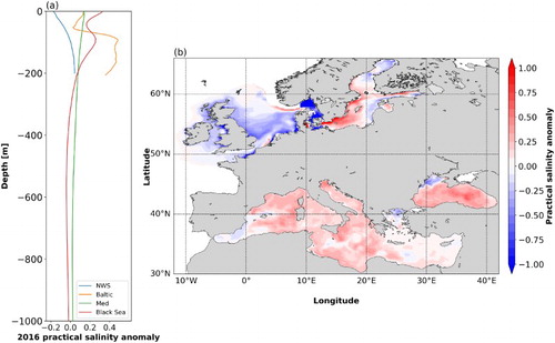
The Black Sea presents relatively homogeneous positive surface and subsurface (<200 m) salinity anomalies centred in the eastern gyre, except along the north-western coasts close to the Danube river delta linked to a more intense runoff during 2016 (Figure 1.1.8).

In the Baltic Sea, strong negative sea surface salinity anomalies are found in the Skagerrak, Kattegat and the Danish Straits (details on the dynamics and impact of Baltic Sea inflow variations are given in Section 3.7). As a cautionary note, it must be stressed that the sea surface salinity results from the Baltic reanalysis are inconsistent with both the global model and the model for the North-West Shelf, possibly due to the use of different numerical circulation models, as well as to differences in the data assimilation systems and hydrological and meteorological forcing.

The North-West Shelf area is characterised by rather uniform negative sea surface salinity anomalies, with values getting stronger close to the Seine and the Elbe river mouths, with the exception of the Rhine, where positive anomalies are recorded (Figure 1.1.8(b)). On average over the area, 2016 was fresher in the upper 100 m compared to the 1993–2014 mean, with a salinity value of 0.17 lower at the surface, while below 100 m the salinity exceeded the 1993–2014 mean (Figure 1.1.8(a)).

1.2. Sea level

Leading author: Jean-François Legeais

Contributing authors: Karina von Schuckmann, Angelique Melet, Andrea Storto, Benoit Meyssignac

Statement of outcome: Global mean sea level has risen at a rate of 3.3 mm/year over the 1993–2016 period. After a rapid increase in 2015, the rate of rise has slightly weakened in 2016 due to neutral El Niño Southern Oscillation conditions. At the regional scale, the spatial extent of the El Niño Southern Oscillation signature observed in the equatorial Pacific Ocean has been reduced in 2016 compared to previous years. During 2016, positive and negative anomalies have been observed with respect to the climatology in the Baltic Sea and the Mediterranean Sea respectively. The TOPEX-A instrumental drift (1993–1998) has been quantified by several recent studies, highlighting that its correction would lead to an acceleration of the global mean sea level rate of change during the altimetry era.

Products used:

Table

Ref. no.	Product name and type	Documentation
1.2.1	DUACS (Data Unification and Altimeter Combination System) delayed-time altimeter daily sea level products, Remote sensing	http://climate.copernicus.eu/climate-data-store

Since 1993, satellite altimetry measurements have allowed the analysis of sea level evolution at different spatial and temporal scales (Legeais et al. 2016; Pujol et al. 2016; Ablain et al. 2017; Cipollini et al. 2017a; Escudier et al. 2017).

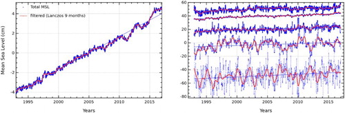
The trend of global mean sea level during 1993–2016 amounts to 3.3 mm/year (Table 1.2.1 and Figure 1.2.1; see also IPCC 2013; Nerem et al. 2017, Chambers et al. 2017 and Legeais et al. 2018). The altimeter mean sea level trend is corrected for the Glacial Isostatic Adjustment (−0.3 mm/year) to take into account the changes of the geoid over the ocean due to the Post Glacial Rebound (Peltier 2004; Tamisiea and Mitrovica 2011; Spada 2017). The global mean sea level trend uncertainty is ±0.5 mm/year (Ablain et al. 2015). The main sources of errors are related to several altimeter geophysical standards (Legeais et al. 2014, Couhert et al. 2014), the instabilities of the altimeter parameters (Ablain et al. 2012) and the multi-mission calibration (Zawadzki and Ablain 2016). Between 1993 and 1998, the global mean sea level has been known to be affected by an instrumental drift in the TOPEX-A measurements which has been quantified by several studies (Valladeau et al. 2012; Watson et al. 2015, Dieng et al. 2017; Beckley et al. 2017). Accounting for the TOPEX-A instrumental correction, these studies provided a revised global mean sea level record with a significant reduction of the associated trend during 1993–2015 (from 3.3 to 3.0 mm/year) but with a clear acceleration from 1993 to the present. Using the corrected global mean sea level time series, Dieng et al. (2017) and Chen et al. (2017) found improved closure of the sea level budget compared to the uncorrected data. However, there is not yet consensus on the best approach to estimate the drift correction at global and at regional scales. The recommendation of the 2017 Ocean Surface Topography Science Team has been to use the on-going reprocessing of the TOPEX measurements to compute the global mean sea level in the future. Therefore, the altimeter mean sea level provided here is not corrected for the TOPEX-A drift.

Figure 1.2.1. Temporal evolution of globally (left) and regionally (right) averaged daily mean sea level without annual and semi-annual signals (blue) and 9-month low-pass filtered mean sea level (red) anomalies relative to the 1993–2014 mean. Arbitrary offsets have been introduced for more clarity. From top to bottom, the regions are North-West Shelf, Iberia–Biscay–Ireland, Mediterranean (Med.) Sea, Black Sea and Baltic Sea. The mean sea level curves have been corrected for the Glacial Isostatic Adjustment using the ICE5G-VM2 model (Peltier 2004). See Table 1.2.1 for the definition of the dataset.

The contribution of the steric signal to the total sea level trend (one-third) and the associated uncertainty has been discussed by Legeais et al. (2016). An updated analysis of the steric sea level is provided in Section 2.2 of this issue and MacIntosh et al. (2017) provide a discussion of its uncertainty. The steric contribution of the deep ocean is expected to be significantly smaller, as suggested by the nearly zero residual trend obtained with the budget closure approach of Dieng et al. (2017).

Significant interannual variations are observed on the global MSL time series (Figure 1.2.1, left) and contribute to the global MSL trend uncertainty in addition of all sources of errors described earlier. The link between these variations and the El Niño Southern Oscillation has been discussed by Legeais et al. (2016). Additional analysis of this link can be found in Ablain et al. (2017) and new insights are provided in Section 2.6 of this issue. Focusing on the recent evolution, Figure 1.2.1 shows that after the rapid increase in 2015, the global mean sea level rise has slightly reduced in 2016 corresponding to a neutral ENSO index.

The altimeter mean sea level trends observed in the different CMEMS regions are positive and relatively close to each other, except in the Baltic Sea where a higher trend is observed (Table 1.2.1 and Figure 1.2.1, right). The time series have been corrected for regional estimates of the GIA using the ICE5G-VM2 GIA model (Peltier 2004). In the CMEMS regions discussed here, the thermosteric contribution to the sea level (up to 50% in the Mediterranean Sea, Legeais et al. 2016) is greater than the one observed at the global scale (about 30%). During 2016, an increasing and decreasing sea level is observed in the North-West Shelf region and Black sea respectively (Figure 1.2.1, right), whereas the sea level records in other regions show a steady evolution. The origins of the altimeter trend uncertainty at regional scale have been presented by Legeais et al. (2016). The first origin is the altimetry errors that can be related to the reduced quality of the altimeter sea level estimation in coastal areas (Cipollini et al. 2017b) and to the greater error of some geophysical altimeter corrections (ocean tide and atmospheric corrections). The second contributor is related to the large sea level variability induced by the internal variability of the climate system (and the fact that the associated trend may vary with the length of the record). The local variability is generated by regional changes in winds, surface atmospheric pressure and ocean currents which averaged out at the global scale (e.g. Stammer et al. 2013) but this can significantly contribute to the MSL uncertainty at the basin scale. In coastal areas, the set up and run up of the waves also contribute to the local variability (Melet et al. 2016). Both altimetry errors and uncertainty in the trend estimate due to interannual variations are included in the uncertainties indicated in Table 1.2.1. They explain why significantly greater interannual variations are found in the Baltic Sea and to a reduced extent in the Mediterranean and Black Seas (semi-enclosed basins) than in the North-West Shelf and Iberia–Biscay–Ireland regions (larger, deeper and open-ocean areas) (see Figure 1.2.1, right panel). Despite its significant associated uncertainty, the mean sea level evolution in the Baltic Sea has been demonstrated to be correlated with the heat flux at the entrance of the basin (Major Baltic Inflow, see Section 3.7).

Table 1.1.1. Products used for the surface and subsurface temperature and salinity analyses.

Ref. no.	Product name and type	Documentation
1.1.1	SST_GLO_SST_L4_NRT_OBSERVATIONS_010_001 Remote sensing, in situ	PUM: http://marine.copernicus.eu/documents/PUM/CMEMS-OSI-PUM-010-001.pdf; QUID: http://marine.copernicus.eu/documents/QUID/CMEMS-OSI-QUID-010-001.pdf; Donlon et al. (2012)
1.1.2	SST_GLO_SST_L4_REP_OBSERVATIONS_010_011 Remote sensing, in situ	PUM: http://marine.copernicus.eu/documents/PUM/CMEMS-OSI-PUM-010-011.pdf; QUID: http://marine.copernicus.eu/documents/QUID/CMEMS-OSI-QUID-010-011.pdf; Roberts-Jones et al. (2012)
1.1.3	SST_BAL_SST_L4_REP_OBSERVATIONS_010_016 Remote sensing	PUM: http://marine.copernicus.eu/documents/PUM/CMEMS-OSI-PUM-010-016.pdf; QUID: http://marine.copernicus.eu/documents/QUID/CMEMS-OSI-QUID-010-016.pdf
1.1.4	SST_BAL_SST_L4_NRT_OBSERVATIONS_010_007_b Remote sensing	PUM: http://marine.copernicus.eu/documents/PUM/CMEMS-OSI-PUM-010-007-b.pdf; QUID: http://marine.copernicus.eu/documents/QUID/CMEMS-OSI-QUID-010-003-007-008.pdf
1.1.5	SST_MED_SST_L4_REP_OBSERVATIONS_010_021 and SST_BS_SST_L4_REP_OBSERVATIONS_010_022 Remote sensing	PUM: http://marine.copernicus.eu/documents/PUM/CMEMS-OSI-PUM-010-021-022.pdf QUID: http://marine.copernicus.eu/documents/QUID/CMEMS-OSI-QUID-010-021-022.pdf Pisano et al. (2016)
1.1.6	SST_MED_SST_L4_NRT_OBSERVATIONS_010_004 and SST_BS_SST_L4_NRT_OBSERVATIONS_010_006 Remote sensing	PUM: http://marine.copernicus.eu/documents/PUM/CMEMS-OSI-PUM-010-004-006-012-013.pdf QUID: http://marine.copericus.eu/documents/QUID/CMEMS-OSI-QUID-010-004-006-012-013.pdf Buongiorno Nardelli et al. (2013)
1.1.7	SST_NWS_SST_L4_REP_OBSERVATIONS_010_023 Remote sensing	PUM: http://marine.copernicus.eu/documents/PUM/CMEMS-OSI-PUM-010-023.pdf QUID: http://marine.copernicus.eu/documents/QUID/CMEMS-OSI-QUID-010-023.pdf
1.1.8	GLOBAL_REP_PHY_001_021 In situ, remote sensing	PUM: http://marine.copernicus.eu/documents/QUID/CMEMS-GLO-PUM-001-021.pdf QUID: http://marine.copernicus.eu/documents/PUM/CMEMS-GLO-QUID-001-021.pdf Guinehut et al. (2012); Droghei et al. (2016); Droghei et al. (2018)
1.1.9	GLOBAL_REANALYSIS_PHY_001_026 Reanalysis	PUM: http://marine.copernicus.eu/documents/PUM/CMEMS-GLO-PUM-001-026.pdf QUID: http://marine.copernicus.eu/documents/QUID/CMEMS-GLO-QUID-001-026.pdf
1.1.10	MEDSEA_REANALYSIS_PHYS_006_004 Reanalysis	PUM: http://marine.copernicus.eu/documents/PUM/CMEMS-MED-PUM-006-004.pdf QUID: http://marine.copernicus.eu/documents/QUID/CMEMS-MED-QUID-006-004.pdf DOI: https://doi.org/10.25423/medsea_reanalysis_phys_006_004 Citation: Simoncelli et al. (2014)
1.1.11	NORTHWESTSHELF_REANALYSIS_PHYS_004_009 Reanalysis	PUM: http://marine.copernicus.eu/documents/PUM/CMEMS-NWS-PUM-004-009-011.pdf QUID: http://marine.copernicus.eu/documents/QUID/CMEMS-NWS-QUID-004-009-011.pdf
1.1.12	NORTHWESTSHELF_ANALYSIS_FORECAST_PHYS_004_001_b Model	PUM: http://cmems-resources.cls.fr/documents/PUM/CMEMS-NWS-PUM-004-001.pdf QUID: http://cmems-resources.cls.fr/documents/QUID/CMEMS-NWS-QUID-004-001
1.1.13	BLKSEA_REANALYSIS_PHYS_007_004 Reanalysis	PUM: http://marine.copernicus.eu/documents/PUM/CMEMS-BS-PUM-007-004.pdf QUID: http://marine.copernicus.eu/documents/QUID/CMEMS-BS-QUID-007-004.pdf
1.1.14	BALTICSEA_REANALYSIS_PHY_003_008 Reanalysis	PUM: http://marine.copernicus.eu/documents/PUM/CMEMS-BAL-PUM-003-008.pdf QUID: http://marine.copernicus.eu/documents/QUID/CMEMS-BAL-QUID-003-008.pdf

Table 1.2.1. Mean sea level trends and their uncertainty in the period 1993–2016 for the global ocean and different CMEMS regions for the total altimeter sea level.

Regions	Mean sea level trend (1993–2016) (mm/year)
	Total (GIA corrected)
Global ocean	3.3 ± 0.5
NW shelf	2.6 ± 0.8
IBI	3.3 ± 0.5
Med. Sea	2.7 ± 0.9
Black Sea	2.8 ± 2.5
Baltic Sea	4.0 ± 2.9

Note: The altimeter trends have been corrected for the glacial isostatic adjustment using the ICE5G-VM2 model (Peltier 2004). Results are based on the Data Unification and Altimeter Combination System (DUACS) delayed-time altimeter sea level products (two satellites constellation) distributed within the Copernicus Climate Change Service (C3S). These C3S sea level maps are based on a stable number of altimeters (two) in the satellite constellation.

The regional sea level trends during 1993–2016 can deviate considerably from the global mean (values range spatially between −5 and +5 mm/year around the 3 mm/year global estimate). This is explained by various geophysical processes partially attributed to natural internal climate variability and to anthropogenic forcing (Meyssignac et al. 2012; Palanisamy et al. 2015; Han et al. 2017). The large-scale variations of the altimeter mean sea level trends during 1993–2016 (Figure 1.2.2, left) have been discussed in Legeais et al. (2016), showing that the high trends observed in the western tropical Pacific Ocean (up to + 8 mm/year) are mainly of thermosteric origin (Meyssignac et al. 2017). The regional sea level trend uncertainty is of the order of 2–3 mm/year with values as low as 0.5 mm/year or as high as 5.0 mm/year depending on the regions (Ablain et al. 2015; P. Prandi, personal communication).

Figure 1.2.2. Spatial distribution of the total sea level trends during 1993–2016 (in mm/year) in the global ocean (left) and the European Seas (right). No Glacial Isostatic Adjustment correction is applied on the altimeter data. See Table 1.2.1 for the definition of the dataset.

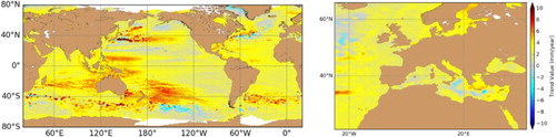
In the European region, relatively homogeneous trends can be found in the North-West Shelf and Iberia–Biscay–Ireland regions (∼2–3 mm/year) (Figure 1.2.2, right). In the open ocean, these trends are essentially related to thermosteric effects (Legeais et al. 2016) but halosteric effects through evaporation and precipitation changes can also significantly contribute to sea level trends (e.g. in the Atlantic) (e.g. Durack & Wijffels 2010). Larger total sea level trends are found in the Baltic Sea (up to 6.0 mm/year). However, as mentioned above, less confidence is attributed to the sea level estimation in this region. In the Mediterranean Sea, the different trend patterns observed in the Adriatic Sea, Aegean Sea and the Eastern basin have been discussed by Legeais et al. (2016). The link with recurrent gyres has been highlighted, especially the Ierapetra gyre in the Levantine basin and the large change in circulation (the Eastern Mediterranean transient) in the Ionian Sea.

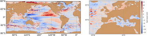
The sea level anomaly field for 2016 compared to the 1993–2014 climatology is dominated by the dipole (±) observed in the equatorial Pacific Ocean associated with ENSO (Schiermeier 2015) (Figure 1.2.3, left). While in 2015, the positive anomaly observed in the East of the basin reached the coast of Alaska (see Figure 13 of Legeais et al. 2016), here its northward extension has been reduced. In the Baltic Sea, the origin of the observed positive anomaly (Figure 1.2.3, right) has been linked to a major inflow event (Mohrholz et al. 2015) that took place in 2015–2016. Section 3.7 describes the link between the major Baltic inflows, the sea level and bottom salinity in this basin. In the Mediterranean Sea, a lower sea level has been observed in 2016 compared to its climatological mean over the entire basin, except in the Algerian basin (see Section 3.4). This is not observed in Figure 1.2.1 (right) where the trend is included. Such a basin-wide pattern can be related to a response to changes in mass flux through the Strait of Gibraltar forced by the wind (Fukumori et al. 2007 and Section 3.3) but also to the interannual variability observed in this region (Pinardi & Masetti 2000).

Figure 1.2.3. Global (left) and regional (right) spatial variability of the difference between the detrended altimeter mean sea level during 2016 and 1993–2014. See Table 1.2.1 for the definition of the dataset.

1.3. Currents

Leading authors: Marie Drévillon, Jonathan Tinker, Romain Bourdallé-Badie, Eric Greiner

Contributing authors: Hélène Etienne, Marie-Hélène Rio, Yann Drillet, Fabrice Hernandez

Statement of main outcomes: Surface current interannual variability is a signature of large-scale climate regimes or variability modes. At the global scale, the tropical currents are the strongest signal in the mean state for 1993–2014 as well as in the 2016 anomaly. The signature of the decaying 2015/2016 El Niño in the Tropical Pacific is the strongest feature of the global 2016 current anomaly. At mid-latitudes eastward flowing currents are reinforced in 2016, and at the regional scale in the North-Western European shelf of the North Atlantic, the wind regimes strongly influence 2016 current.

Products used:

Table

Ref. no.	Product name and type	Documentation
1.3.1	GLOBAL_REANALYSIS_PHY_001_025 Reanalysis	PUM: http://marine.copernicus.eu/documents/PUM/CMEMS-GLO-PUM-001-025.pdf QUID: http://marine.copernicus.eu/documents/QUID/CMEMS-GLO-QUID-001-025.pdf
1.3.3	NORTHWESTSHELF_REANALYSIS_PHYS_004_009 Reanalysis	PUM: http://marine.copernicus.eu/documents/PUM/CMEMS-NWS-PUM-004-009-011.pdf QUID: http://marine.copernicus.eu/documents/QUID/CMEMS-NWS-QUID-004-009-011.pdf
1.3.4	NORTHWESTSHELF_ANALYSIS_FORECAST_PHYS_004_001_b Near-Real-Time analysis	PUM: http://cmems-resources.cls.fr/documents/PUM/CMEMS-NWS-PUM-004-001.pdf QUID: http://cmems-resources.cls.fr/documents/QUID/CMEMS-NWS-QUID-004-001-002.pdf

Several new developments with respect to the first issue of the Ocean State Report are included in this section. At the global scale only significant anomalies (stronger than interannual variability signals excluding the ‘outlier’ 1997/1998 El Niño) are shown. Wind anomalies are shown in support of the analysis, at the global scale as for the North-West European Shelf Seas. Trends are not shown in this section but they are analysed in Section 2.7, as western boundary currents indicators rely on trends, and figures from this section also support the analysis of the western boundary currents 2016 anomaly.

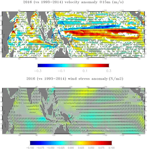
When comparing the 15 m depth climatology of current velocity (1993–2014) and the value for 2016 in Figure 1.3.1, one can note that the major signals of 2016 are located in the equatorial Pacific and the Indian Ocean. Velocity anomalies in Figure 1.3.2 confirm that significant large-scale signals (larger than the average interannual variability over 1993–2014) appear in 2016 in these areas. These large signals are associated with the El Niño event of winter 2015/2016 (Drévillon et al. 2016), which was still active during the first half of 2016 (Section 2.6). In 2015, and associated with the 2015/2016 El Niño event (see Drévillon et al. 2016), the acceleration of the North Equatorial Counter Current and the slowing down of the westward South Equatorial Current were associated with a slowing down of the trade winds mostly in the Central Equatorial Pacific. The 2016 surface current anomalies were weaker on global average than the 2015 current anomalies. In the western tropical Pacific in 2016 as shown in Figure 1.3.2, trade winds accelerated north of the equator while they decelerated south of the equator. As with the wind stress anomalies, the acceleration of the South Equatorial Current in the western Tropical Pacific started at the beginning of 2016 (not shown). In the Eastern part of the Tropical Pacific, the eastward North Equatorial Counter Current slowed down while the South Equatorial Current was reinforced mostly during the second half of 2016 (not shown).

Figure 1.3.1. 15 m Current velocity (m/s) from GLORYS reanalysis at ¼° (product reference 1.3.1). Upper Panel: 1993–2014 Climatology of current velocity. Lower Panel: 2016 annual average values of current velocity.

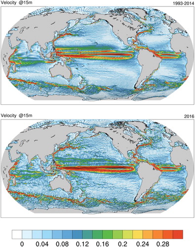
Figure 1.3.2. Upper panel: current velocity anomaly near 15 m (m/s) in 2016, with respect to the 1993–2014 climatology computed from the GLORYS reanalysis at ¼° CMEMS product reference 1.3.1 (colour shading, NB: only significant deviations are shown, which are greater than one standard deviation of the interannual variability, computed on the 1993–2014 period omitting 1997 and 1998); direction of the 1993–2014 climatological currents computed from CMEMS product reference 1.3.1 (black vectors). Lower panel: ECMWF ERA-interim wind stress anomalies (N/m²) with respect to 1993–2014 wind stress climatology (colour shading), and direction of the 1993–2014 climatological wind stress (black vectors).

In the Indian Ocean, the slowing down of the Java Current occurred mostly during the second half of the year (while it flows westward according to Schott and McCreary 2001) and the Indian South Equatorial Current also decelerated, which was consistent with a slowing down of the transports in the Indonesian Throughflow, and with transports in that area as depicted in Section 2.3.

At mid-latitudes, the increase of the eastward surface currents was present throughout the year 2016, and was consistent with anomalously strong westerlies, especially during winter. The surface currents in the North-Western European shelf of the North Atlantic Ocean are discussed in the following, and the 24-year trends in sub-tropical western boundary currents are analysed in Section 2.7.

We focus now on the North-West European shelf seas average surface currents, which are strongly linked to the surface winds. The 2016 annual mean wind was very similar to climatology (shown as streamlines in Figure 1.3.3) in terms of magnitude, and large-scale pattern (Figure 1.3.4). In winter, south of ∼54°N, the wind was stronger than in the climatological period (greater than the 80th percentile values), with a more westerly direction. In the summer, the wind was close to climatology, with a band of stronger winds around England and Ireland, and a small region of weaker winds around Shetland (Figure 1.3.4).

Figure 1.3.3. Surface wind and currents (CMEMS product reference 1.3.3) for the 1994–2013 climatology, 2016 (CMEMS product reference 1.3.4), and the anomaly (2016 – climatology). Mean surface current and wind: annual, winter (December–February), and summer (June–August) mean (left to right) for the 1994–2013 climatology (upper row), 2016 (middle row), and the 2016 anomaly (2016-climatology, bottom row). Streamlines show the 10 m winds (streamline colour (with inset colour bar) shows wind magnitude). The (log scale) map colouring shows the surface current magnitude (metre per second) with the current directions given with vectors. These are shaded off the shelf.

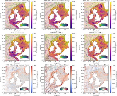
In the annual mean, the 2016 surface magnitude of the shelf break current (north of ∼54°N, and particularly in winter), the Dooley Current (eastward North Sea Current at ∼58°N) and the Norwegian Coastal Current were all greater than in the climatological period (Figure 1.3.4), but were not as strong as they were in 2015 (c.f. Figure 40 in Tinker et al. 2016). Surface currents in most of the central and southern North Sea were close to climatology, as were the surface currents in the western English Channel, while the eastern English Channel had stronger currents than climatology. Overall, the surface current magnitudes were weaker in the Celtic Sea, and stronger in the Irish Sea, than in the climatology.

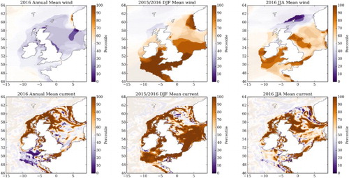
Figure 1.3.4. The 2016 surface wind and current magnitude as a percentile of 1994–2013 (CMEMS product reference 1.3.3) baseline: where 2016 wind and surface current (CMEMS product reference 1.3.4) magnitude fit within the distribution of values from 1994 to 2013, for the annual mean, winter (December–February, for 2015/2016) and summer (June–August) (left to right), for the magnitude of the 10 m wind and surface currents (upper row and lower row, respectively). These are shaded off the shelf. To highlight the extreme values, the values from the centre of the distribution (within 20th to 80th percentile) are lightly greyed out. For example, dark brown colouring indicating that the wind magnitude is at the 90th percentile of the 1994–2013 climatology period shows that 2016 was windier than most years within the climatology period.

The summer and winter mean surface current fields show seasonal differences from the annual mean. The winter (December 2015 to February 2016) surface current magnitudes were generally stronger than the climatology, although were close to climatology in the northern North Sea – consistent with the surface wind anomaly pattern. In winter 2015, when the surface current magnitudes were also stronger than climatology in most parts of the region, some southern regions such as the English Channel and the southern North Sea were close to climatology. In contrast, in 2016 these regions have some of the greatest positive winter magnitude anomalies (currents stronger than the 80th percentile of the climatology period), particularly through the Dover Straits (perhaps reflecting an enhanced exchange between the English Channel and the North Sea, associated with a strong wind anomaly blowing along the English Channel, e.g. Figure 1.3.3).

The 2016 summer surface current magnitudes were generally greater than climatology to the north of Ireland and Scotland, through the central northern North Sea (∼56–60°N, including the Dooley Current, the North Atlantic inflow water and the adjacent Norwegian Coastal Current). The surface magnitudes were also greater than climatology from the central English Channel across the southern North Sea towards the German Bight. Most other regions were fairly close to climatology (Figures 1.3.3 and 1.3.4).

1.4. Sea ice

Leading authors: Annette Samuelsen, Gilles Garric, Roshin P. Raj, Lars Axell, Hao Zuo, K. Andrew Peterson, Signe Aaboe

Contributing authors: Andrea Storto, Thomas Lavergne, Lars-Anders Breivik

Statement of outcome: For the last two decades, the sea-ice extent has been decreasing in the Arctic and slowly increasing in the Antarctic at a rate of about ∼780,000 km²/decade. The long-term sea-ice volume follows roughly the sea-ice extent. In 2016, however, the Antarctic had a large drop in both sea-ice extent and volume towards the end of the year, with sea-ice extent 4 standard deviations below the long-term mean in December. The decrease continues in the Arctic in 2016 and we see reduction compared to the long-term mean throughout the year. The Baltic has lower than normal sea-ice extent compared to the past three years. In the present OSR, we include modelled sea-ice volume in addition to sea-ice extent from both model and satellite. We also estimate uncertainties based on an ensemble of global models.

Products used:

Table

Ref. no.	Product name and type	Documentation
1.4.1	GLOBAL_REANALYSIS_PHY_001_026 Reanalysis	QUID: http://marine.copernicus.eu/documents/QUID/CMEMS-GLO-QUID-001-026.pdf PUM: http://marine.copernicus.eu/documents/PUM/CMEMS-GLO-PUM-001-026.pdf
1.4.2	ARCTIC_REANALYSIS_PHYS_002_003 Reanalysis	QUID: http://marine.copernicus.eu/documents/QUID/CMEMS-ARC-QUID-002-003.pdf PUM: http://marine.copernicus.eu/documents/PUM/CMEMS-ARC-PUM-002-ALL.pdf
1.4.3	Operational ice charts from SMHI (planned to be part of the CMEMS catalogue in the future)	http://www.smhi.se/klimatdata/oceanografi/havsis; Uiboupin et al. (2010)
1.4.4	SEAICE_GLO_SEAICE_L4_REP_OBSERVATIONS_011_009 Remote sensing	PUM: http://marine.copernicus.eu/documents/PUM/CMEMS-OSI-PUM-011-009.pdf QUID: http://marine.copernicus.eu/documents/QUID/CMEMS-OSI-QUID-011-001to007-009to012.pdf

Since the first issue of the Ocean State Report, sea-ice volume has been introduced as a new key climate indicator for high latitudes in order to better monitor and assess the drastic changes currently taking place in the Polar Regions. In the Antarctic, sea ice has shown a slow, steady increase in both extent and volume, but in 2016 a sharp decrease was seen (Figure 1.4.2(b)). In September 2016, when the extent was still within one standard deviation of the 1993–2014 climatological mean, the sea-ice extent shows the strongest decrease in the sector bordering the western Indian Ocean and parts of the Pacific, while the March extent decreased most in regions close to the Ross and Amundsen seas, the Weddell Sea and in the [0°–30°E] coastal areas (Figure 1.4.1(b)). However, the largest decrease was seen in the three last months of 2016 with the sea-ice extent being more than 4 standard deviations, below the long-term mean in December 2016 and about 3 standard deviations below the long-term mean in November 2016. The large sea-ice anomaly is associated with anomalously large surface heat flux throughout the year and anomalous north-westerly winds in the Atlantic and Pacific sectors (see Section 4.1 for more details).

Figure 1.4.1. (a) Map of sea-ice extent for the Arctic including the 1993–2014 climatology for, March 2016, September 2016, and the September minimum of 2012 (CMEMS product reference 1.4.1 (March) and 1.4.2 (September)). (b) Same as (a) but for the Antarctic Ocean, and with the September maximum of 2014 shown (CMEMS product reference 1.4.1).

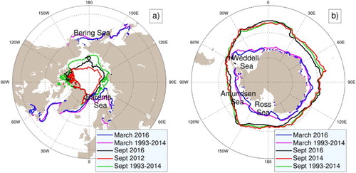
Arctic sea-ice extent in 2016 remains largely below the 1993–2014 climatology in all seasons (Figure 1.4.3(a)). In the Arctic, the downward trend of both sea-ice extent and sea-ice volume as reported in Samuelsen et al. (2016) continues during the year 2016 (Figure 1.4.2(a)). The September sea-ice extent is about half way between the long-term mean (1993–2014) and the observed September minimum during the year 2012 (Figure 1.4.1(a)), however with a larger decrease in the region of the Beaufort Sea compared to the long-term mean. The March sea-ice extent in 2016 has particularly decreased in the Bering and Barents seas compared to the long-term mean. The decrease is connected to an anomalously large oceanic heat flux into the Arctic and some regional driving forces in 2016 (Section 4.1). The Arctic sea-ice volume (based on reanalysis, CMEMS product reference 1.4.1) showed an increase during 2013–14, but during 2016 the volume reaches, with 2012, the lowest 1993–2015 values (Figure 1.4.2(a)). Sea-ice volume plays an important role for freshwater content in the Arctic (see Section 2.10).

Figure 1.4.2. Time series for the period 1993–2016 of the monthly sea-ice extent anomaly (blue) and volume anomaly (red) (mean seasonal cycle has been removed) relative to the 1993–2014 climatology. For (a) the Arctic (CMEMS product reference 1.4.1 (volume) and 1.4.4 (extent)), (b) the Antarctic (CMEMS product reference 1.4.1 (volume) and 1.4.4 (extent)) and (c) for the Baltic Sea (product reference 1.4.3).

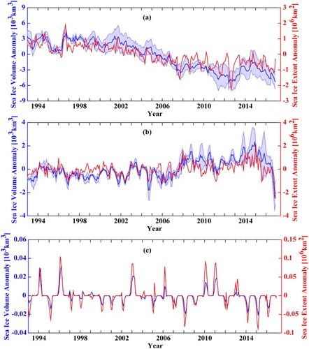
Sea-ice extent in the Baltic Sea was relatively low in 2016, but higher than in 2015 (Figures. 1.4.2c and 1.4.3c). Temporal changes of sea-ice volume and extent in the Baltic Sea follow each other much more closely than what is reported for the two other regions, probably because the Baltic Sea only has first-year ice. In the Baltic, the sea-ice trend over 1993–2016 was a decrease of 4.6 × 10³ km²/decade in extent and a decrease of 2.16 km³/decade in volume.

Table 1.4.1. Trend values over the 1993–2016 period for sea-ice extent and sea-ice volume at annual rate.

	Arctic		Antarctic
	Extent 10^6 km^2/decade	Volume 10^3 km^3/decade	Extent 10^6 km^2/decade	Volume 10^3 km^3/decade
Trend for product reference 1.4.4	−0.85		0.42
Trend for product reference 1.4.1	−0.78	−3.51	0.2	0.68
Uncertainty for product reference 1.4.1	0.07	0.32	0.1	0.15

Sea-ice concentration and extent are more easily monitored by remote sensing than sea-ice thickness which, although estimates based on SMOS (Tian-Kunze et al. 2014) and altimetry exist, is associated with higher uncertainty (approximately 30%) related to assumptions in the thickness calculation such as snow cover and ice and snow densities (Zygmuntowska et al. 2014; Ricker et al. 2014). A model intercomparison focusing on sea ice in the Arctic also shows that sea-ice thickness is a variable where there is large disagreement between the models (Chevallier et al. 2016). The initial efforts to reduce this uncertainty by assimilating sea-ice thickness into models have begun (Kauker et al. 2015; Xie et al. 2016) showing promising results in order to improve model estimates, as well as improving model forecasts of sea-ice extent and cover. The uncertainty values listed in Table 1.4.1 are based on an ensemble of 4 reanalyses (CMEMS product reference 1.4.1) and yield an uncertainty of about 10% for both Arctic sea-ice extent and volume. This is less than what was found for sea-ice volume in Chevallier et al. (2016), but here we use data from global simulations using the same ocean model with the same resolution and forcing, and three of them also use the same ice model. In contrast, Chevallier et al. (2016) used 14 different systems, with several using different ocean and ice models along with differing atmospheric forcing. The four-system uncertainty used here is a better estimation of observational and forcing uncertainty. Although all the reanalyses assimilate sea-ice concentration, the spread of the sea-ice extent trend from reanalysis ensemble remains higher than the spread found for a longer period between individual satellite algorithms (Ivanova et al. 2014).

1.5. Ocean colour

Leading authors: Shubha Sathyendranath, Silvia Pardo

Contributing authors: Mario Benincasa, Vittorio E. Brando, Robert J.W. Brewin, Frédéric Mélin, Rosalia Santoleri

Statement of outcome: An increasing trend in chlorophyll concentration is observed in the European Seas in the period 1998–2016, with the exception of the Black Sea. Annual anomalies show the subregional distributions of those trends, with remarkable east–west differences over the Mediterranean Sea. Global chlorophyll trend analysis shows an increasing trend in high latitudes and a decreasing trend in tropical areas over the past 18 years.

Products used:

Table

Ref. No.	Product name & type	Documentation
1.5.1	OCEANCOLOUR_ARC_CHL_L3_REP_OBSERVATIONS_009_069 Remote sensing	PUM: http://marine.copernicus.eu/documents/PUM/CMEMS-OC-PUM-009-ALL.pdf QUID: http://marine.copernicus.eu/documents/QUID/CMEMS-OC-QUID-009-066-067-068-069-088-091.pdf
1.5.2	OCEANCOLOUR_ATL_CHL_L3_REP_OBSERVATIONS_009_067 Remote sensing	PUM: http://marine.copernicus.eu/documents/PUM/CMEMS-OC-PUM-009-ALL.pdf QUID: http://marine.copernicus.eu/documents/QUID/CMEMS-OC-QUID-009-066-067-068-069-088-091.pdf
1.5.3	OCEANCOLOUR_BAL_CHL_L3_REP_OBSERVATIONS_009_080 Remote sensing	PUM: http://marine.copernicus.eu/documents/PUM/CMEMS-OC-PUM-009-ALL.pdf QUID: http://marine.copernicus.eu/documents/QUID/CMEMS-OC-QUID-009-080-097.pdf
1.5.4	OCEANCOLOUR_BS_CHL_L3_REP_OBSERVATIONS_009_071 Remote sensing	PUM: http://marine.copernicus.eu/documents/PUM/CMEMS-OC-PUM-009-ALL.pdf QUID: http://marine.copernicus.eu/documents/QUID/CMEMS-OC-QUID-009-038to045-071-073-078-079-095-096.pdf
1.5.5	OCEANCOLOUR_MED_CHL_L3_REP_OBSERVATIONS_009_073 Remote sensing	PUM: http://marine.copernicus.eu/documents/PUM/CMEMS-OC-PUM-009-ALL.pdf QUID: http://marine.copernicus.eu/documents/QUID/CMEMS-OC-QUID-009-038to045-071-073-078-079-095-096.pdf
1.5.6	OCEANCOLOUR_GLO_CHL_L3_REP_OBSERVATIONS_009_065 Remote sensing	PUM: http://marine.copernicus.eu/documents/PUM/CMEMS-OC-PUM-009-ALL.pdf QUID: http://cmems-resources.cls.fr/documents/QUID/CMEMS-OC-QUID-009-064-065-093.pdf

In this chapter, we use the Ocean Colour Climate Change Initiative (OC-CCI) remote sensing reflectance data to study the trends and anomalies in phytoplankton over the last 18 years (time series not sufficiently long to extract climate-change signal unequivocally). The OC-CCI Version 3.1 used here is a merged product that incorporates data from SeaWiFS, MODIS-A, MERIS and VIIRS data (Sathyendranath et al. 2017). Algorithms were selected for atmospheric correction after a round-robin comparison of candidate algorithms (see Müller et al. 2015; Sathyendranath et al. 2017; Sathyendranath et al. 2018). The data were band-shifted and bias-corrected at the level of the remote sensing reflectance, to avoid inter-sensor biases, and to produce reflectance data at a consistent set of wavebands, using SeaWiFS as the reference sensor.

The OC-CCI chlorophyll concentration (a measure of phytoplankton abundance) is calculated using a blended algorithm (Jackson et al. 2017). In the OC-CCI product suite, chlorophyll algorithm was implemented first by using a fuzzy-logic optical classification scheme to identify the membership of various optical classes in each pixel; then the best performing algorithm for each of the optical classes is applied to the remote sensing reflectance at that pixel, and finally, the computed values are weighted according to class membership, to yield the chlorophyll concentration for that pixel. These OC-CCI products were used for the global analyses.

The OC-CCI remote sensing reflectance data were used by CMEMS Ocean Colour Thematic Assembly Centre (OC-TAC) to compute chlorophyll concentration (a measure of phytoplankton concentration), using algorithms optimised for the European waters. The products optimised for European waters were used for analyses at the level of European waters. A description of the regional chlorophyll algorithms can be found in the corresponding CMEMS Quality Information Documents (QuID), referenced below. The trends and anomalies are calculated globally, and for the CMEMS regions around Europe.

Figure 1.5.1(a–e) shows the time series data for the five CMEMS regions. The red line in each subplot shows a simple, linear fit to the data, show the general trend. No correction for outliers was applied to the data. Nor was any seasonal signal removed before calculating the trend. We note that the linear trend is positive for all regions (chlorophyll increasing with time), except for the Black Sea, with different slopes for each of the region. Furthermore, the underlying data show that the interannual variability in the different CMEMS regions does not show the same pattern. The interannual variation in the Arctic Region (Figure 1.5.1(c)) shows a broad curve that appears to peak at around 2008–2012, with the chlorophyll concentration decreasing afterwards. A similar pattern is seen in the Baltic Region (Figure 1.5.1(b)). The Atlantic region, on the other hand, shows a steady increasing trend till about 2014–2016 (Figure 1.5.1(d)), similar to the Mediterranean Region (Figure 1.5.1(e)). Finally, the Black Sea (Figure 1.5.1(a)) shows little interannual variation throughout the study period.

For comparison with the CMEMS regions, we also show the corresponding time series data for two ecological provinces as defined by Longhurst (2006). The Western Pacific Warm Pool (WARM, Figure 1.5.2(a)) province shows clear evidence of 3–4 year cycles in the data, perhaps tied to the ENSO, which is not evident in any of the CMEMS regions. But the Arabian Sea (ARAB, Figure 1.5.2(b)) province, similar to the CMEMS regions, shows double peaks in chlorophyll each year (two blooms per year), with the highest values appearing in the 2002–2005 period, with weak-to-no interannual variation in recent years.

The global anomalies for 2016 are shown in Figure 1.5.3(a). Most of the open-ocean waters of the Atlantic Basin (North and South) shows regions of positive anomalies (or no significant change) compared with the climatology, with negative anomalies evident in the western tropical Atlantic, European waters and coastal regions off western Africa. In contrast, tropical waters of both the Pacific and the Indian Oceans show vast regions with negative anomalies, with the notable exception of a patch of positive anomaly off South-West India. More positive anomalies appear as one moves towards the Southern Ocean, with very high positive anomalies appearing close to the Antarctic. The positive anomalies are more pronounced in the Pacific than in the Indian Ocean sector of the Southern Ocean.

The anomalies in the CMEMS regions are shown in more detail in Figure 1.5.3(b–f). The Arctic Region (Figure 1.5.3(c)) shows mostly negative anomalies except in the Atlantic sector. The anomalies in the Black Sea (Figure 1.5.3(f)) are negative, whereas those in the Mediterranean (Figure 1.5.3(d)) show an east–west divide pattern (negative in the west and positive in the east). The North-West Atlantic Region (Figure 1.5.3(b)) shows positive anomalies except for the European waters, which show mostly negative anomalies. The anomalies in the Baltic (Figure 1.5.3(e)) show pronounced regional differences, with the western part being dominated by negative anomalies, the eastern parts by positive anomalies and weak anomalies in between.

The global trends in chlorophyll concentration (Figure 1.5.4) were calculated for every 4 × 4 km pixel, for the entire study period (September 1997–December 2016). The trend detection method is based on the Census-I algorithm as described by Vantrepotte et al. (2009), where the time series is decomposed as a fixed seasonal cycle plus a linear trend component plus a residual component. Noting that Mélin et al. (2017) calculated trends from October 1997 to September 2015, the similarities between the two results are very consistent. We note great swaths of the tropical ocean where the trends are negative, but higher latitudes show strong positive anomalies, with the notable exception of the South Pacific sub-tropical gyre core. Most of the northern and tropical Indian Ocean shows negative anomalies.

1.6. Nitrates

Leading authors: Coralie Perruche, Cosimo Solidoro

Contributing authors: Stefano Salon

Statement of outcome: In this new section in chapter one of the Ocean State Report, the distribution of nitrate – a macro-nutrient limiting primary production – is studied over the 1993–2016 period. We show that its interannual variability between 40°S and 40°N strongly correlates with El Niño Southern Oscillation. During 2016, a negative anomaly emerged in equatorial Pacific due to the reduced intensity of equatorial upwelling. In the Mediterranean Sea, a negative anomaly occurred in 2016 which is possibly due to stronger water column stratification.

Products used:

Table

Ref. no.	Product name and type	Documentation
1.6.1	GLOBAL_REANALYSIS_BIO_001_018 Reanalysis	PUM: http://marine.copernicus.eu/documents/PUM/CMEMS-GLO-PUM-001-018.pdf QUID: http://marine.copernicus.eu/documents/QUID/CMEMS-GLO-QUID-001-018.pdf
1.6.2	MEDSEA_REANALYSIS_BIO_006_018 Reanalysis	PUM: http://marine.copernicus.eu/documents/PUM/CMEMS-MED-PUM-006-008.pdf QUID: http://marine.copernicus.eu/documents/QUID/CMEMS-MED-QUID-006-008.pdf

Figure 1.6.1 presents the surface concentration of nitrate computed from the CMEMS global biogeochemical reanalysis (product reference 1.6.1). The 30°S–30°N distribution is characterised by undetectably low concentrations of nitrates in sub-tropical oligotrophic gyres except in a rich tongue in the equatorial Pacific. This depletion in surface waters of oligotrophic gyres is due to a permanent stratification that induces a very limited entrainment of nitrates within the shallow well-lit mixed layer. These small amounts of nitrates are immediately utilised by phytoplankton. The nitrate tongue in tropical Pacific and along eastern boundaries coasts are induced by the equatorial and coastal upwelling (vertical velocities) of deep nitrate-rich waters. At higher latitudes, the mixed layer deepening in winter entrains large amounts of nitrates within it.

If we now consider the 2016 anomaly on Figure 1.6.2, we see a large negative anomaly which can be attributed to the 2016 El Niño event which reduces the intensity of the equatorial upwelling and the vertical supply of nitrates (Radenac et al. 2001). Nitrate-poor waters of the Western Pacific are advected eastward. The cold tongue of the tropical Pacific is referred to an HNLC region (High Nutrient/Low Chlorophyll). This low phytoplankton biomass relative to available nitrate concentrations in the euphotic layer is explained by micronutrient limitation, namely iron. This nitracline deepening during El Niño years is thus associated with ferricline deepening (Radenac et al. 2001; Wang et al. 2005) and with a negative anomaly of chlorophyll (see Figure 1.5.3 in Section 1.5). The time series of the nitrate anomaly (signal previously detrended and deseasonalised) over 40°S–40°N region (Figure 1.6.3) shows a strong correlation between nitrate concentration and ENSO index.

At the regional scale, other processes can play important roles in shaping nutrient distribution. As an interesting example, the Mediterranean Sea (Figure 1.6.4(a), product reference 1.6.2) shows a spatial pattern of nutrient distribution that depends on the superposition of inverse estuarine circulation of the Atlantic water inflowing from the Gibraltar Straits, local areas of upwelling (i.e. north-western Mediterranean Sea and Southern Adriatic Sea), an uneven distribution of rivers, and – most importantly – the activity of plankton autotrophs, which depletes nutrient concentration along the Atlantic modified water while enriching through their sinking the outflowing deeper waters (i.e. the clearly shown east to west gradient in the subsurface 0–150 m map, Figure 1.6.4(b)). In 2016, the anomaly map (Figure 1.6.4(c)) highlights a generally lower than average value of nitrate concentration, more evident in specific areas (e.g. north-western Mediterranean, south-eastern Tyrrhenian Sea, north-western Ionian Sea, south-eastern Aegean Sea, central Levantine), which is related to a general negative anomaly of the mixed layer depth (not shown), and therefore to a stronger water column stratification. The positive anomaly observed along the Italian coast of the Adriatic Sea is related to the 2016 phytoplankton negative anomaly, as prescribed by the assimilated ocean colour chlorophyll (Figure 1.5.3) and the climatological (i.e. constant in years) nutrient river discharge rates.

1.7. Air-to-sea carbon flux

Leading authors: Coralie Perruche, Cosimo Solidoro

Contributing authors: Gianpiero Cossarini

Statement of outcome: In this new section of the Ocean State Report, we study the sea-to-air CO₂ flux as described by a global and a regional coupled physical-biogeochemical model. At the global scale, the model simulates a relatively stable ocean carbon uptake during the 1990s and a sharp increase since the beginning of the 2000s. In the Mediterranean Sea, model results indicate that it acts as a weak sink during the last decade. In 2016, there is a strong negative anomaly of the equatorial Pacific outgassing due to a weaker upwelling (end of El Niño event).

Products used:

Table

Ref. no.	Product name and type	Documentation
1.7.1	GLOBAL_REANALYSIS_BIO_001_018 Reanalysis	PUM: http://marine.copernicus.eu/documents/PUM/CMEMS-GLO-PUM-001-018.pdf QUID: http://marine.copernicus.eu/documents/QUID/CMEMS-GLO-QUID-001-018.pdf
1.7.2	MEDSEA_REANALYSIS_BIO_006_018 Reanalysis	PUM: http://marine.copernicus.eu/documents/PUM/CMEMS-MED-PUM-006-008.pdf QUID: http://marine.copernicus.eu/documents/QUID/CMEMS-MED-QUID-006-008.pdf

The concentration of atmospheric CO₂ has exceeded 400 ppm in 2015 and has thus increased by about 40% from about 280ppm in the pre-industrial era (Conway et al. 1994, Masarie and Tans 1995, www.esrl.noaa.gov/gmd/ccgg/trends/). This increase would have been much stronger without the contribution of the ocean and land biospheres which absorb each year roughly one half (25% ocean and 25% land) of the anthropogenic carbon emissions (Le Quéré et al. 2016, Ballantyne et al. 2012). The CO₂ flux is directly linked to the CO₂ partial pressure (pCO₂) in the ocean (product no. 1.7.1, 1.7.2) and in the atmosphere, but also to CO₂ solubility in sea water and to wind speed (Sarmiento and Gruber 2006, Takahashi et al. 2002, Wanninkhof 1992).

A few processes called ‘pumps’ are driving the air–sea exchange of CO₂ and the vertical distribution of carbon in the ocean. The ocean CO₂ partial pressure is prominently controlled by the physico-chemical pump of solubility which increases as temperature and salinity fall. CO₂-enriched water masses are then trapped below the thermocline where deep water convection occurs. As a consequence, the solubility pump is stronger at high latitudes. The second pump is the so-called ‘organic carbon pump’, which refers to biological processes that sustain a vertical downward flux of carbon (Sarmiento and Gruber 2006, Gehlen et al. 2011). Through photosynthesis, phytoplankton absorbs dissolved inorganic carbon (DIC) in the surface sunlight layer (euphotic zone) to build organic matter, which is then remineralised in the ocean interior into DIC after particle sinking. The third pump – the ‘carbonate pump’ – has a negative feedback on ocean carbon uptake as it counteracts the downward flux of DIC into the deep ocean (Gehlen et al. 2011). This process involves calcifiers – plankton species such as coccolithophores (phytoplankton) or foraminifera (zooplankton). To build their carbonate shell, they absorb DIC and release CO₂.

The superposition of those pumps results in large regional variability in the distribution of the sea-to-air flux of CO₂. Figure 1.7.1 is a climatological mean of these CO₂ fluxes computed from the CMEMS global biogeochemical reanalysis product (product reference 1.7.1). The ocean acts as a carbon sink at high latitudes (40–60° in both hemispheres) due to the combined effect of cooling/formation of deep water in winter and of biological activity (strong seasonal bloom in this area) in spring (Takahashi 2002). High wind speeds over these low pCO₂ waters increase the ocean uptake (Takahashi 2002). In upwelling systems (equatorial upwelling, eastern boundary upwelling system, Arabian Sea upwelling), the ocean is a source of CO₂ for the atmosphere due to the upwelling of CO₂-rich waters (Figure 1.7.1). In the Pacific Ocean, the upwelled water masses at the equator are then advected westward and poleward due to equatorial divergence within the sub-tropical cells (Schott et al. 2004). Besides this climatological view, there is a strong interannual variability, in particular in regions with strong climate modes (Resplandy et al. 2015), i.e. Pacific Decadal Oscillation, North Atlantic Oscillation, Southern Annual Mode in high latitudes and El Niño Southern Oscillation in tropical Pacific. In 2016, a significant negative CO₂ flux anomaly in the tropical Pacific (Figure 1.7.2) highlights the signature of El Niño during the beginning of the year (see Figure 2.6.1 of Section 2.6: this CO₂ flux anomaly is associated with a positive anomaly of surface temperature). The less intense upwelling leads to reduced outgassing in the tropical Pacific.

Atmospheric measurements and CO₂ emission inventories show a global increase of ocean and land carbon uptake over the past 50 years (Ballantyne et al. 2012, Le Quéré et al. 2017). In the framework of the Global Carbon Project (http://www.globalcarbonproject.org/about/index.htm), an annual assessment of the global budget is done each year (Le Quéré et al. 2017). During the last decade (2007–2016), anthropogenic air-to-sea carbon flux amounts to 2.4 ± 0.5 PgC/year (Le Quéré et al. 2017). In 2016, the ocean sink was 2.6 ± 0.5 PgC/year (Le Quéré et al. 2017). These global budget estimations (Le Quéré et al. 2017) are based on observations from the 1990s (mean) and on Earth System Models (annual anomalies and trends). Figure 1.7.3 presents the model estimation of the net integrated sea-to-air carbon flux compared with estimates of Landschützer et al. (2014) and Rödenbeck et al. (2015) based on data-driven mapping methods applied on SOCAT database (surface ocean pCO₂ measurements: http://www.socat.info/, Bakker et al. 2014). It shows a good comparison between these products with a relatively stable ocean carbon uptake during the 1990s and a sharp increase since the beginning of the 2000s. This may be related to a weakening of the upper-ocean overturning circulation (DeVries et al. 2017), but needs further investigations. In 2016, our model simulates a global ocean uptake of 2.2 PgC/year. To obtain the global anthropogenic atmosphere-ocean CO₂ flux, we have to add the natural river outgassing of 0.45 PgC/year (Jacobson et al. 2007). It gives an anthropogenic CO₂ flux of 2.65 PgC/year that is in line with Le Quéré et al.’s (2017) estimation.

The different estimations of the global air–sea carbon flux agree on the current buffer capacity of the ocean to alleviate the greenhouse effect and the associated climate warming. A lot of uncertainties still remain in the different estimates of the global flux due to the scarcity of data and the coarse resolution/complexity of physical and biogeochemical processes in models. But Earth System Models (Roy et al. 2011; Ciais et al. 2013 (IPPC WG1, chapter 6); Séférian et al. 2014) ultimately predict a decrease of ocean carbon uptake due to the warming of surface layers (decrease of CO₂ solubility) (Roy et al. 2011), enhanced ocean stratification (less ventilation and carbon export by mixing) (Séférian et al. 2012) and biogeochemical processes (ocean acidification, deoxygenation, reduced primary productivity) (Bopp et al. 2013) in the next century. However, the ocean response to the climate change is still a matter of debate.

By offering products that result from the combination of state-of-the-art observations and higher resolution models specifically designed to describe the characteristics of a given system, CMEMS regional systems can provide more accurate analyses and forecasts of a regional area making them ideally placed to inform this debate going forward. Figure 1.7.4 illustrates the spatial distribution of the mean climatological annual pCO₂ (ppm) and net air–sea fluxes for CO₂ (gC/m²/y) over the period 1999–2014 in the Mediterranean Sea (product reference 1.7.2).

Results of the Mediterranean regional reanalysis provide a more detailed description of the spatial variability in the regional sea, especially along the shelves, which are known to be important when computing carbon budgets at the global scale (Bauer et al. 2013, Bourgeois et al. 2016). Reanalysis results indicate that in the last decade, the Mediterranean Sea, as a whole, acted as a weak sink of atmospheric carbon (around −3.5 TgC/year in average over the 1999–2014 period). Furthermore, we observe that while the climatology derived from the Mediterranean model returns a more detailed picture of the spatial distribution of CO₂ fluxes over the Mediterranean Sea in respect of the one provided by the global model, both climatologies agree in indicating that there was an outgassing on the southern parts of the Mediterranean Basin and an ocean uptake in its northern parts. In this context it is worth noting that biological activity plays a significant role in carbon sequestration ecosystem services in the Mediterranean Sea: as an example, Melaku Canu et al. (2015) showed that without it the Mediterranean would be a globally significant source of CO₂, and quantified the contribution of plankton carbon sequesteration value between €100 and €1500 million annually for the Mediterranean Sea.

Since direct experimental observations of pCO₂ are too scarce and do not cover the basin scale, it is not possible to have a direct assessment of the errors on this parameter. However, it is possible to derive an indirect estimate of the uncertainty on pCO₂ by combining the uncertainties on alkalinity and on DIC, and using the error propagation equation. This produces a conservative estimate of pCO₂ uncertainty in the surface layer of about 50ppm. The uncertainties on alkalinity and DIC were produced by comparing observation-based climatologies to model-based climatologies (QUID of product reference 1.7.2).

The pCO₂, and the related CO₂ atmospheric fluxes, shows a strong seasonal cycle (Figure 1.7.5) as linked to temperature changes and trophic dynamics. Superposed are interannual changes (Figure 1.7.5) which may be related to interannual variability in physical or biogeochemical parameters, but also to changes in the input and exchanges with the system boundaries, i.e. linked to properties of Atlantic water inflowing from Gibraltar straits (Cossarini et al. 2015).

Figure 1.7.5(b) highlights both the seasonal and interannual variability, and shows that over the last 15 years there is a slightly negative multiannual trend in the basin means of the sea-to-air CO₂ flux which is the response to the increase of atmospheric pCO₂ from 360 to 399 (data of Lampedusa station from World Data Centre for Greenhouse gases 2017). Spatial distributions also vary from year to year, in response to changes in biological productivity, surface temperature and transport processes. Anomalous changes during the year 2016 (rel. to the 1999–2014 reference period) indicate that in the last year the fluxes from the atmosphere to the ocean are slightly higher (Figure 1.7.5(a)) compared to the climatological mean (i.e. the mean annual value of 2016 equals to −3.5 gC/m²/year). As it can be seen from the anomaly map (Figure 1.7.5), differences are not homogenously distributed in space, but depend on, and track effects of, general circulation and even mesoscale features. In particular, one can observe Atlantic water spreading into the western part of the Mediterranean and along the African coast, as well as relevant changes in the Levantine basin, which are possibly related to the temperature regime, and positive anomalies in the Adriatic Sea and along the coasts of the Ionian and Levantine seas.

1.8. Wind

Leading author: Ad Stoffelen

Contributing authors: Jos de Kloe, Ana Trindade, Daphne van Zanten, Anton Verhoef, Abderahim Bentamy

Statement of outcome: Global and regional decadal trends in marine wind and stress forcing are now available through stable satellite instrument records, providing more detailed evidence of the changing climate. In 2016, a prominent anomaly stands out in the Arctic region over the Atlantic with poleward winds, specifically for the months of September, October and November.

Products used:

Table

Ref. No.	Product name & type	Documentation
1.8.1	WIND_GLO_WIND_L3_NRT_OBSERVATIONS_012_002 Remote sensing	PUM: http://marine.copernicus.eu/documents/PUM/CMEMS-OSI-PUM-012-002.pdf QUID: http://marine.copernicus.eu/documents/QUID/CMEMS-OSI-QUID-012-002-003-005.pdf
1.8.2	WIND_GLO_WIND_L3_REP_OBSERVATIONS_012_005 Remote sensing	PUM: http://marine.copernicus.eu/documents/PUM/CMEMS-OSI-PUM-012-002.pdf, QUID: http://marine.copernicus.eu/documents/QUID/CMEMS-OSI-QUID-012-002-003-005.pdf
1.8.3	WIND_GLO_WIND_L4_NRT_OBSERVATIONS_012_004 Remote sensing	PUM: http://marine.copernicus.eu/documents/PUM/CMEMS-OSI-PUM-012-004.pdf QUID: http://marine.copernicus.eu/documents/QUID/CMEMS-OSI-QUID-012-002-003-005.pdf
1.8.4	WIND_GLO_WIND_L4_REP_OBSERVATIONS_012_003 Remote sensing	PUM: http://marine.copernicus.eu/documents/PUM/CMEMS-OSI-PUM-012-003.pdf QUID: http://marine.copernicus.eu/documents/QUID/CMEMS-OSI-QUID-012-002-003-005.pdf
1.8.5	EUMETSAT OSI SAF L2 CDRs Remote sensing	http://projects.knmi.nl/scatterometer/archived_prod/ : ERS 25 km (1991-2000), doi:10.15770/EUM_SAF_OSI_0009; QuikScat 25 km (1999-2009), doi:10.15770/EUM_SAF_OSI_0002 QuikScat 50 km (1999-2009), doi:10.15770/EUM_SAF_OSI_0003 ASCAT-A 12.5 km (2007-2016), doi:10.15770/EUM_SAF_OSI_0007 ASCAT-A 25 km (2007-2016), doi:10.15770/EUM_SAF_OSI_0006 OceanSat-2 scatterometer (2009-2014), in preparation.
1.8.6	ERA-interim U10s Reanalysis (atmosphere)	doi:10.21944/ERA-Interim_U10S

The former Ocean and Sea-ice Thematic Assembly Centre (OSI TAC) (since replaced with 3 separate TACs) provides homogeneous long-term wind and stress products to help marine users and Marine Forecasting Centers to extract the relevant variability information from scatterometer and radiometer instrument observation records (Vogelzang et al. 2011; Belmonte Rivas et al. 2017; Stoffelen et al. 2017a; Stoffelen et al. 2017b; Wang et al. 2017; Verhoef et al. 2017a; Wentz et al. 2017). In addition, collocated operational (Sandu et al. 2013) or ERA-interim (Dee et al. 2011) atmospheric model fields are provided.

Whereas globally observed scatterometer winds have been very stable over the last 30 years (Verhoef et al. 2017a, 2017b), local decadal changes can easily be as large as 1 m/s (Verhoef et al. 2017a), due to local or regional flow regimes, such as the North Atlantic Oscillation and El Nino (e.g. Sprintall et al. 2014). The collocated model reanalysis record is less stable and showing some spurious trends, most likely due to changing observational input over the years (Verhoef et al. 2017a, 2017b).

Wind and wind stress curl products can now be analysed for a stable ASCAT-A sample from 2007 to 2014 and include comparisons between ASCAT-A and model reanalyses, thanks to the collocation procedure. An ASCAT-A climatology from this period is compared to the mean over 2016 in Figure 1.8.1.

The figure shows the largest effect in the Pacific at medium latitudes, where the westerlies were reinforced over 2016. Also, the medium-latitude southern hemisphere (SH) shows zonal enhancement over 2016, but this happened to a much lesser extent in the Atlantic Northern Hemisphere (NH), although the associated cool sea surface temperature anomalies are similar at these northern mid-latitudes in the Pacific and Atlantic. In the Atlantic basin, zonal anomalies appear relatively small over 2016. In the southern hemisphere Pacific, the tropical and sub-tropical easterlies were weaker over 2016 due to the El Niño Southern Oscillation. As a consequence and in line with the sea surface temperature anomalies (Section 1.1, Figure 1.1.2), weaker easterlies are also observed in the Indian Ocean.

Figure 1.8.2 zooms into the polar region and shows a clear Atlantic anomaly in 2016, specifically for the months September, October and November, for the meridional wind component. 2016 clearly stands out as there is a poleward flow, while all other years show flow away from the North Pole, which aligns more with its overall strong cooling in autumn. This wind anomaly is associated with an anomalously slow growth of autumn sea-ice cover in the polar seas (Section 1.4, Figure 1.4.3(a)), enhanced ocean water flow towards the pole (Section 4.1), warm sea surface temperature (Section 1.1, Figure 1.4.2), but also with enhanced cloudiness, which limits the polar winter cooling. The observed meridional wind anomaly is much stronger than the anomaly in the collocated model reanalysis data (not shown). Meridional wind anomalies (not shown) were also associated with the anomalous sea-ice conditions in the Antarctic over September 2016 in particular (Section 4.1).

Figure 1.4.3. Seasonal cycle of sea-ice extent: Long-term mean (1993–2014) in blue, one standard deviation (blue shading) and monthly means for 2016 in red for (a) Arctic (CMEMS product reference 1.4.4), (b) Antarctic (CMEMS product reference 1.4.4) and (c) Baltic Sea (product reference 1.4.3).

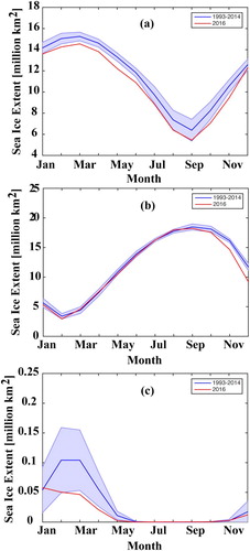
Figure 1.5.1. Regional time series (1997–2016) for (a) Black Sea, (b) Baltic Sea, (c) Arctic Ocean, (d) North Atlantic Ocean and (e) Mediterranean Sea.

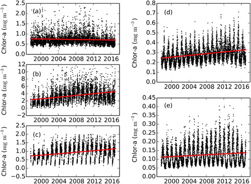
Figure 1.5.2. Province time series (1997–2016) for (a) WARM and (b) ARAB provinces.

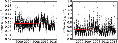
Figure 1.5.3. Chlorophyll anomalies for 2016 relative to the 1997–2014 reference period for (a) North Atlantic Ocean, (b) Arctic Ocean, (c) Global Ocean, (d) Mediterranean Sea, (e) Baltic Sea and (f) Black Sea.

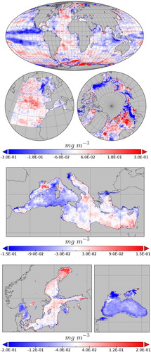
Figure 1.5.4. Global chlorophyll trend map (September 1997 to December 2016). Only statistically significant (p < .05) trends are shown.

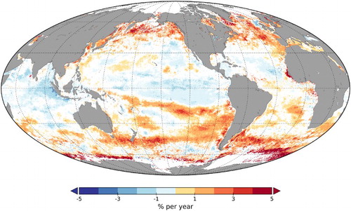
Figure 1.6.1. Map of surface nitrates (mmol/m³) computed from the CMEMS global reanalysis product (see text for more details) over the period 1993–2014 (log scale).

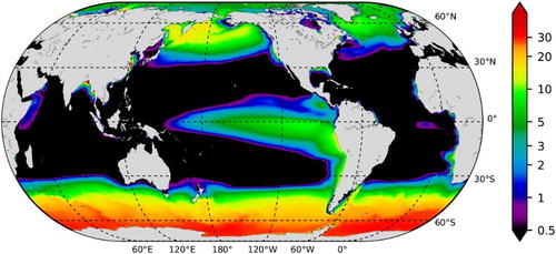
Figure 1.6.2. Anomalies of surface nitrates (mmol/m³) in 2016 relative to climatological period 1993–2014. At each grid cell, the time series was previously detrended. Our simulation starting from WOA and GLODAP climatologies and being relatively short, we prefer removing the trend to filter the model drift.

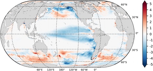
Figure 1.6.3. (Green – left axis) Surface nitrates mean over 40°S–40°N region (mmol/m⁻³). Signal previously detrended and deseasonalised with a monthly 1993–2014 climatology. (Black – right axis) The monthly multivariate ENSO index (MEI), downloaded from the NOAA website (https://www.esrl.noaa.gov/psd/enso/mei/). Note that the sign of the ENSO index is inverted (El Niño years correspond to negative values).

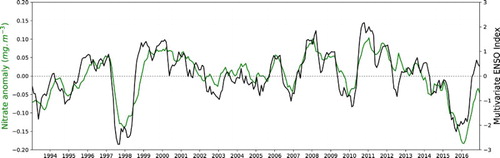
Figure 1.6.4. Surface (a) and subsurface (b, 0–150 m) maps of nitrate (mmol/m³) computed from the CMEMS Mediterranean reanalysis product (see text for more details) over the period 2002–2014. Anomalies of surface nitrate (c, mmol/m³) in 2016 relative to climatological period 2002–2014.

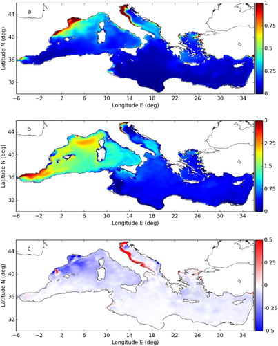
Figure 1.7.1. Net sea-to-air flux for CO₂ (mol. C/m²/year) computed from the CMEMS global reanalysis (product reference 1.7.1) over the period 1993–2014. Positive values represent a flux from the ocean to the atmosphere (outgassing).

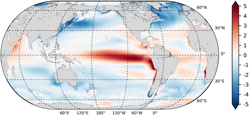
Figure 1.7.2. Anomalies of net sea-to-air flux of CO₂ (mol. C/m²/year) in 2016 relative to climatological period 1993–2014. At each grid cell, the time series was previously detrended. Our simulation starting from WOA and GLODAP climatologies and being relatively short, we prefer removing the trend to filter the model drift.

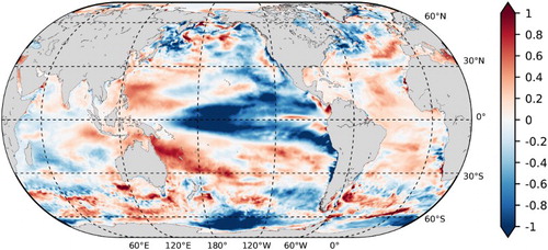
Figure 1.7.3. Annual time series of net sea-to-air flux of CO₂ (PgC/year). (Blue) Landschützer et al. (2014) product: a neural network is used to reconstruct the non-linear relationship between external drivers (SST, SSS, MLD, Chla and atmospheric pCO₂) and SOCATv2 pCO₂ database. Downloaded on the SOCOM (Surface Ocean pCO₂ Mapping intercomparison) website: http://www.bgc-jena.mpg.de/SOCOM/ (black) Rödenbeck et al. (2015) product: statistical interpolation scheme with SOCATv3 pCO₂ database. (RED), the CMEMS global reanalysis (product reference 1.7.1).

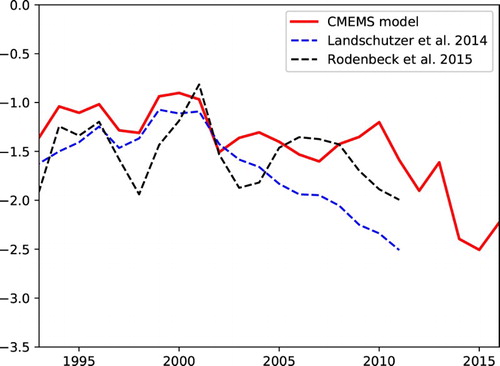
Figure 1.7.4. Climatological mean (1999–2014) of ocean pCO₂ (a, ppm) and net sea-to-air flux for CO₂ (b, mol. C/m²/year, positive values represent a flux from the ocean to the atmosphere, i.e. outgassing) derived from product reference 1.7.2.

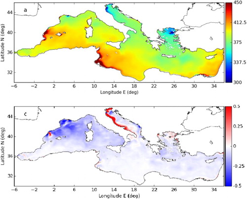
Figure 1.7.5. (a) Anomalies during 2016 (relative to the climatology reference shown in Fig. 1.7.4) of net sea-to-air CO₂ flux (mol. C/m²/year) derived from the product reference 1.7.2. (b) Monthly (green line) and annual mean (red line) sea-to-air CO₂ fluxes (mmolC/m²/d, first axis, positive values represent a flux from the ocean to the atmosphere, i.e. outgassing) and monthly ocean partial pressure of CO₂ (pCO₂, [ppm], blue line, second axis) for the years 1999–2016. Values refer to spatial averages over the entire Mediterranean Sea basin, and are derived from product no. 1.7.2.

Figure 1.8.3 shows wind stress curl anomalies globally in 2016 and zooms into the North Pole region, which would affect and describe the interaction and dynamics of the atmosphere, ocean and sea ice. Clearly, the wind stress curl was enhanced over the North Pole region during 2016. Following the large Pacific, zonal wind anomaly around 45°N in Figures. 1.8.1 and 1.8.3 indeed shows a generally positive shear contribution to the curl to the north and a negative shear to the south in line with expectations. More generally, scatterometer wind stress curl and divergence structures are smaller scale (down to 25 km) and higher amplitude than the structures observed in the collocated model reanalysis seasonal and annual maps (not shown) in line with Chelton et al. (2004), due to resolved air–sea interaction processes, including due to moist convection.

Figure 1.8.1. 2016 Anomaly of the zonal wind with respect to the 2007–2014 climatology for the ASCAT-A wind scatterometer by latitude and segregated with respect to ocean basin: Atlantic (green), Pacific (black) and Indian (blue) (product reference 1.8.2).

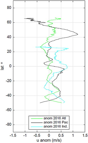
Figure 1.8.2. Mean meridional (poleward) wind component for the months September, October and November by latitude for the years 2007 through 2016 as derived from ASCAT-A (product reference 1.8.2).

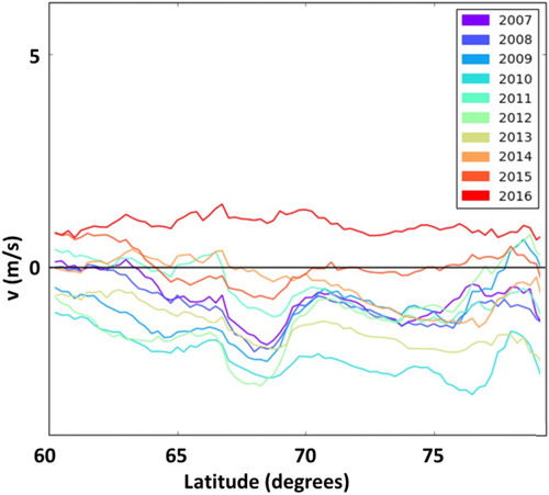
Figure 1.8.3. Wind stress curl anomaly of 2016 with respect to the climatology from 2007 through 2014 as computed from ASCAT-A (product reference 1.8.2) in units of 10⁻⁶/s.

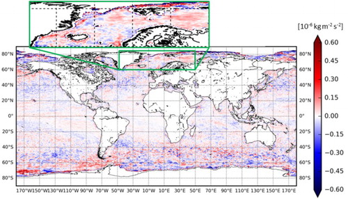
Chapter 2 – Changes in ocean climate

This chapter is dedicated to monitoring marine environmental conditions characterising the blue, white and green ocean state, variability and changes over the period 1993–2016, with a specific focus on anomalous changes during 2016. We first examine specific topics at a global or European scale, which are known to play a considerable role in the balance of changes in the Earth system. Specifically, the oceans play a fundamental role as Earth system regulator to anthropogenic pressure and natural forcing due to their capacity to store large quantities of heat. Monitoring of the global and European ocean heat storage (Section 2.1) is therefore important as its changes additionally affect the stratification, the ocean currents, the thermal memory (Hansen et al. 2011), ice melt (Polyakov et al. 2017), climate adjustments such as Earth surface temperature (Dieng et al. 2017), air–sea interactions as well as marine ecosystems and human livelihoods (Doney et al. 2012). The link between thermal volume changes and contemporary sea level change is also specifically addressed (Section 2.2). Another fundamental characteristic of the ocean in the Earth system is its capacity to redistribute large amounts of heat and mass around the globe. In this context, ocean heat and mass transports are monitored at well-known choke points in the world ocean (Section 2.3). The oceans supply more than 50% of oxygen in the Earth’s atmosphere through photosynthesis by phytoplankton (microscopic plants) that live in the ocean. Vital monitoring of area extensions with a huge impact on dissolved oxygen (Section 2.4) and phytoplankton growth are then itroduced (Section 2.5).

Specific phenomena are also addressed that occur regionally but are known to affect ocean and Earth climate at a global and European scale. These include the El Niño Southern Oscillation (ENSO), which is one of the most important sources of global natural climate variability (Section 2.6). Extratropical western boundary currents are regions of largest air–sea fluxes of heat, moisture and carbon dioxide in the world’s oceans and are then discussed (Section 2.7). A specific focus is also delivered on monitoring the Atlantic Meridional Overturning Circulation (AMOC) (Section 2.8), which is well known to have fundamental impact on global and European climate (e.g. Drijfhout et al. 2012; Woollings et al. 2012). The North Atlantic area is a very sensitive region for changes in ocean climate due to strong air–sea interactions, the AMOC and the formation of new water masses, and specific monitoring tools are delivered for this area (Section 2.9). Finally, the Arctic Ocean is a critical component in the interconnected ‘machine’ that regulates Earth’s climate and a regional analysis on Arctic Ocean freshwater content is discussed (Section 2.10).

2.1. Ocean heat content

Leading authors: Karina von Schuckmann, Andrea Storto, Simona Simoncelli, Roshin P. Raj, Annette Samuelsen, Alvaro de Pascual Collar, Marcos Garcia Sotillo, Tanguy Szerkely.

Contributing authors: Michael Mayer, K. Andrew Peterson, Hao Zuo, Gilles Garric, Maeva Monier.

Statement of outcome: Since the year 1993 the upper (0–700 m) global ocean has warmed at a rate of 0.8 ± 0.1 W/m². We estimate a current Earth energy imbalance of 0.7 W/m² for the period 2005–2016 with a contribution of ∼40% from the 700–2000 m depth layer. Regional 23-year trends (1993–2016) of ocean heat content in European regional seas and the Arctic Ocean show an overall warming which is superimposed by strong year-to-year variability in the North-West-Shelf area. Meridional (North Atlantic, Indian Ocean) and zonal (North Pacific) dipole pattern characterise the ocean heat content anomalies during 2016.

Products used:

Table

Ref. No.	Product name & type	Documentation
2.1.1	GLOBAL_REANALYSIS_PHY_001_026 Reanalysis	PUM: http://marine.copernicus.eu/documents/PUM/CMEMS-GLO-PUM-001-026.pdf QUID: http://marine.copernicus.eu/documents/QUID/CMEMS-GLO-QUID-001-026.pdf
2.1.2	INSITU_GLO_TS_OA_REP_OBSERVATIONS_013_002_b In situ for the year 2016: INSITU_GLO_TS_OA_REP_OBSERVATIONS_013_002_b In situ	PUM: http://marine.copernicus.eu/documents/PUM/CMEMS-INS-PUM-013-002-a.pdf QUID: http://marine.copernicus.eu/documents/QUID/CMEMS-INS-QUID-013-002a.pdf for the year 2016: PUM: http://marine.copernicus.eu/documents/PUM/CMEMS-INS-PUM-013-002-b.pdf QUID: http://marine.copernicus.eu/documents/QUID/CMEMS-INS-QUID-013-002b.pdf
2.1.3	GLOBAL_REP_PHY_001_021 In situ, remote sensing	PUM: http://marine.copernicus.eu/documents/QUID/CMEMS-GLO-QUID-001-021.pdf QUID: http://marine.copernicus.eu/documents/PUM/CMEMS-GLO-PUM-001-021.pdf
2.1.4	MEDSEA_REANALYSIS_PHYS_006_004 In situ	PUM: http://marine.copernicus.eu/documents/PUM/CMEMS-MED-PUM-006-004.pdf QUID: http://marine.copernicus.eu/documents/QUID/CMEMS-MED-QUID-006-004.pdf DOI: https://doi.org/10.25423/medsea_reanalysis_phys_006_004 Citation: Simoncelli et al. (2014)
2.1.5	MEDSEA_REANALYSIS_PHY_006_009 In situ	PUM: http://marine.copernicus.eu/documents/PUM/CMEMS-MED-PUM-006-009.pdf QUID: http://marine.copernicus.eu/documents/QUID/CMEMS-MED-QUID-006-009.pdf DOI: https://doi.org/10.25423/MEDSEA_REANALYSIS_PHY_006_009 Citation: Fratianni et al. (2015)
2.1.6	IBI_REANALYSIS_PHYS_005_002 In situ for the year 2016: IBI_ANALYSIS_FORECAST_PHYS_005_001_b In situ	QUID: http://marine.copernicus.eu/documents/QUID/CMEMS-IBI-QUID-005-002.pdf PUM: http://marine.copernicus.eu/documents/PUM/CMEMS-IBI-PUM-005-002.pdf for the year 2016: QUID: http://marine.copernicus.eu/documents/QUID/CMEMS-IBI-QUID-005-001.pdf PUM: http://marine.copernicus.eu/documents/PUM/CMEMS-IBI-PUM-005-001.pdf
2.1.7	ARCTIC_REANALYSIS_PHYS_002_003 In situ for the year 2016: ARCTIC_ANALYSIS_FORECAST_PHYS_002_001_a In situ	QUID: http://marine.copernicus.eu/documents/QUID/CMEMS-ARC-QUID-002-001a.pdf PUM: http://marine.copernicus.eu/documents/PUM/CMEMS-ARC-PUM-002-ALL.pdf for the year 2016: QUID: http://marine.copernicus.eu/documents/QUID/CMEMS-ARC-QUID-002-003.pdf PUM: http://marine.copernicus.eu/documents/PUM/CMEMS-ARC-PUM-002-ALL.pdf
2.1.8	CERES global mean net flux at the Top-Of-the-Atmosphere Remote sensing	https://ceres.larc.nasa.gov; (Loeb et al. 2009)

Interactions between the atmosphere and the ocean are the key ingredient to adjustments of the Earth’s climate system to oceanic heat changes (e.g. Buckley and Marshall 2016). Ocean heat is affected by and affects atmospheric circulation and the climate (e.g. von Schuckmann et al. 2016a). However, the atmosphere and ocean play a contrasting role in the global energy balance as the latter has a much longer thermal memory (e.g. Levitus et al. 2012). Heat absorbed and redistributed by the ocean can re-emerge at the ocean-atmosphere interface, thereby affecting climate anomalies at multiple time and space scales (Trenberth et al. 2016). Knowing then how much and where heat energy is absorbed and redistributed (Section 2.3) in the ocean, and how, where and when it is finally released are essential issues for understanding the contemporary global climate state, variability and change, as they shape our perspectives for the future.

It is unequivocal that the Earth’s climate is changing and will continue to change, but the magnitude of global warming and regional details are still unclear (IPCC 2013). Because of the accelerated increase of greenhouse gases from human activities since pre-industrial times, heat is accumulated in the climate system and is driving observed global warming (Hansen et al. 2011, 2013). The global ocean plays a critical role in regulating these energy flows (IPCC 2013) and the temporal change of ocean heat content is then one of the fundamental metrics to continually asses the amount of warming in the Earth’s climate system (von Schuckmann et al. 2016a). In addition, energy fluctuations associated with weather systems and clouds, through internal climate modes like ENSO (see Section 2.6), as well as from external influences (solar variations, volcanoes), can additionally cause short-term fluctuations in the Earth’s energy budget (Balmaseda et al. 2013; Mayer et al. 2014; Trenberth et al. 2014).

At a time when pressing questions are being asked by policy-makers concerning the future of Earth’s climate and the evolution of symptoms of climate change, we must understand how much and where the energy is accumulating in order to improve our understanding of the prospects for future climate change (von Schuckmann et al. 2016a). Consequently, one of the priorities of the Copernicus Marine Service Ocean State Report activity is to establish continuous monitoring of global and regional scale ocean heat content changes.

As introduced in the last Ocean State Report (von Schuckmann et al. 2016b), we have obtained ocean heat content anomalies from integrated differences in measured or reanalysed temperature from climatology for the period 1993–2014, and along a vertical profile in the ocean from the surface down to 700 m depth. The calculations are based on a new and innovative approach – the so-called ‘multi-product approach’ (see introduction). We use a combination of ocean reanalyses and observation based products, and all products used are specified in the figure captions. Near-global mean ocean heat content (Figure 2.1.1(a)) shows a continuous increase over the period 1993–2016 at rate of 0.8 ± 0.1 W/m² in the upper 700 m depth layer (see Table 2.1.1), which is slightly higher than the last IPCC estimate of 0.6 W/m² (1993–2010).

Table 2.1.1. Rate of change for global and basin mean ocean heat content, integrated over the upper 700 m (unless indicated otherwise) for the periods as shown (see Figure 0.1 for regional masks and corresponding time series).

Region	1993–2016 trend in W/m^2	2005–2016 trend in W/m^2
Global (60°S–60°N), 0–700 m	0.8 ± 0.1	0.5 ± 0.1
Global (60°S–60°N), 0–2000 m		0.9 ± 0.2
TOA net flux		0.8 ± 0.1
Mediterranean Sea	1.3 ± 0.2
Iberian-Biscay-Irish	0.9 ± 0.4
North-West-Shelf	0.7 ± 0.8
Arctic	0.6 ± 0.1

Note: Uncertainties are computed through bootstrapping, at 99% confidence level.

Rates of ocean heat content over the upper 2000 m depth are delivered only for the period 2005–2016 when the global ocean observing system includes the Argo array measuring to 2000 m in the ice-free ocean (e.g. von Schuckmann and Le Traon 2011; Abraham et al. 2013; Roemmich et al. 2015; Riser et al. 2016). This period is much shorter, and the trend estimates are known to be affected by year-to-year changes such as ENSO and may mask the warming signature (Cazenave et al. 2014). Results show then a warming of 0.5 ± 0.1 W/m² for the upper 700 m depth layer during the period 2005–2016. Integrating down to 2000 m depth increases the warming rate by more than 40% to 0.9 ± 0.2 W/m² (Figure 2.1.1, Table 2.1.1).

Global ocean heat content changes during the past 11 years are further discussed in the context of the physical budget constraint for the Earth’s energy imbalance (von Schuckmann et al. 2016a): on a global scale and at annual to longer time scales, changes in Top-of-the-Atmosphere (TOA) net radiation and rate of ocean heat storage should be in phase and of the same magnitude (Loeb et al. 2012). This is due to the fact that all other forms of heat storage in the Earth system are smaller by factors of 10 than ocean heat storage at these time scales (Trenberth et al. 2016). The 11-year trend of integrated net flux at TOA amounts to 0.8 ± 0.1 W/m² (Table 2.1.1). The state of the Earth energy imbalance over the 2005–2016 period as derived from measurements at TOA – and anchored by an independent mean estimate of Earth’s energy imbalance (Loeb et al. 2012) – are in good agreement with global ocean heat content estimates integrated down to 2000 m of depth (Figure 2.1.1, Table 2.1.1), which amounts to 0.6 W/m² over the entire Earth surface. For example, OHC decrease in 2007 and 2010 coincide with reduced net radiative energy input measured at TOA. Taking into account the 0.1 W/m² of abyssal ocean warming (Purkey and Johnson 2010), we estimate the Earth energy imbalance to be 0.7 W/m² over the period 2005–2016 based on ocean heat content. However, some year-to-year differences remain, and their study is beyond the scope of the present section and will be addressed in separate works.

Pronounced ocean heat content increase can also be observed in two regions of the European seas and in the Arctic Ocean (Figure 2.1.2). In the Mediterranean Sea, basin mean upper (0–700 m) ocean heat content rises at a rate of 1.3 ± 0.2 W/m² between 1993 and 2016, which is much stronger compared to the global rate, and compared to what had been estimated in the last Ocean State Report from the observational approach (von Schuckmann al. 2016b). In the Iberian-Biscay-Irish region, area-averaged ocean heat content increases at a rate of 0.9 ± 0.4 W/m² over the past 24 years which is comparable to what was reported last year. An overall warming signal over the past 24 years is observed in the Arctic Ocean, with some variation on multiannual scales. Similar results are reported by Mayer et al. (2016) over the period 2000–2015. The ensemble spread is low and the warming rate of 0.6 ± 0.1 W/m² is significant due to low year-to-year variability in the time series. However, observations in the Arctic are sparse and hence further scientific analyses are needed to assess the robustness of this result.

Year-to-year and longer variability of area-averaged upper (0–700 m) ocean heat content dominates the time series in the European North-West-Shelf region and potentially masks a long-term warming trend (Figure 2.1.2). The time series appear to be affected by a cold anomaly at the beginning of the time series up to the year 2003, changing to positive anomalies until 2014, and again negative anomalies up to the end of the time series in the year 2016. These variations appear to be consistent with observed patterns in the subpolar North Atlantic (see Section 2.9), and future investigations are needed to discuss their nature of origin.

We further investigate regional patterns of ocean heat content change for the period 1993–2016 using the Copernicus Marine Service ‘multi-ensemble approach’. Regional trends show warming at rates ranging from the global mean average (see Table 2.1.1) up to more than 5 W/m² in some specific regions (Figure 2.1.3). There are only a few specific regions where either the warming rate is below the global mean value or we observe a negative trend at rates up to about −3 W/m². These areas are characterised by strong year-to-year variability, such as ENSO in the tropical Pacific area (see Section 2.6), the Southern Ocean or the subpolar North Atlantic area. The latter appears to be linked to observed cooling and freshening in this area as discussed in Sections 1.2, 1.4, 2.9 and 4.3.

The pronounced cold conditions in the subpolar North Atlantic region also persist during 2016 (Figure 2.1.4). Other regions of anomalously cold upper ocean temperatures characterise the changes during 2016. Cold anomalies in the western Pacific warm pool area are linked to the ENSO event during winter 2015/2016, and are further discussed in Section 2.6. The northern subtropical Pacific also shows large patterns of anomalous cold upper ocean temperatures during 2016. In the southern tropical Indian Ocean, a large-scale pattern of anomalous cooling occurs which is not reported elsewhere. Areas of anomalous warm upper ocean heat content can be reported for the eastern subtropical Pacific, the eastern and western subtropical South Pacific, the western and central subtropical Atlantic Ocean (see Section 2.9), and the entire North Indian Ocean.

2.2. Steric sea level

Leading authors: Andrea Storto, Karina von Schuckmann, Jean-François Legeais, Tanguy Szerkely.

Contributing authors: K. Andrew Peterson, Hao Zuo, Gilles Garric.

Statement of main outcome: Thermosteric sea level shows a global rise at a rate of 1.2 ± 0.3 mm/year over the past 11 years (2005–2016). Results reveal a closure of the global sea level budget. Regional 11-year trends of steric sea level show an overall increase, which is masked in areas of high interannual variability such as in the Pacific and North Atlantic area. The latter area is characterised by strong halosteric changes. Meridional (North Atlantic, Indian Ocean) and zonal (North Pacific) dipole pattern characterise the steric sea level anomalies during 2016 driven by thermosteric changes (see Section 2.1).

Products used:

Table

Ref. No.	Product name & type	Documentation
2.2.1	GLOBAL_REANALYSIS_PHY_001_026 Reanalysis	PUM: http://marine.copernicus.eu/documents/PUM/CMEMS-GLO-PUM-001-026.pdf QUID: http://marine.copernicus.eu/documents/QUID/CMEMS-GLO-QUID-001-026.pdf
2.2.2	INSITU_GLO_TS_OA_REP_OBSERVATIONS_013_002_b In situ for the year 2016: INSITU_GLO_TS_OA_REP_OBSERVATIONS_013_002_b In situ	PUM: http://marine.copernicus.eu/documents/PUM/CMEMS-INS-PUM-013-002-ab.pdf; QUID: http://marine.copernicus.eu/documents/QUID/CMEMS-INS-QUID-013-002a.pdf for the year 2016: PUM: http://marine.copernicus.eu/documents/PUM/CMEMS-INS-PUM-013-002-ab.pdf; QUID: http://marine.copernicus.eu/documents/QUID/CMEMS-INS-QUID-013-002b.pdf
2.2.3	GLOBAL_REP_PHY_001_021 In situ, remote sensing	PUM : http://marine.copernicus.eu/documents/QUID/CMEMS-GLO-QUID-001-021.pdf QUID: http://marine.copernicus.eu/documents/PUM/CMEMS-GLO-PUM-001-021.pdf
2.1.4	DUACS delayed-time altimeter daily sea level products (two satellites constellation) Remote sensing	Copernicus Climate Service (C3S) (http://climate.copernicus.eu/climate-data-store)
2.1.5	Global mean ocean mass Remote sensing	http://xena.marine.usf.edu/~chambers/SatLab/Home.html Chambers and Bonin (2012)

Steric sea level is the variation of the ocean volume due to density changes (expansion and contraction of water masses), through ocean salinity (halosteric) and ocean temperature (thermosteric) variations. Thermosteric variability is the dominant component of global steric sea level change (e.g. IPCC 2013; Stammer et al. 2013). Salinity variations associated with freshwater tendencies at the sea surface that are redistributed in the ocean’s interior have a negligible effect on seawater density and thus on sea level changes on the global scale (e.g. Lowe and Gregory 2006). On regional to basin scales, the role of halosteric effects through the addition and subtraction of freshwater or mixing processes can be large, and should not be neglected in sea level studies (e.g. Durack et al. 2014). Regional freshwater changes are found to have an important imprint on global mean sea level (Boening et al. 2012), but their relation to global halosteric sea level changes has not yet been quantified.

There is currently an accumulation of heat in the climate system through a positive Earth's energy imbalance (see Section 2.1), and one of its major symptoms is the observed contemporary sea level rise (von Schuckmann et al. 2016b, see Section 1.5). Thermosteric effects from warming contribute roughly 1/3 of contemporary sea level rise globally (IPCC 2013), and may play even a more important role at a regional scale (e.g. Stammer et al. 2013; Rietbroek et al. 2016). The calculation of steric height between two depth layers h(z ₁, z ₂) involves a vertical integration of ocean density ρ, which in turn can be estimated from temperature T, salinity S and ocean pressure p (ρ(T,S,p)):$h\left(z_1,z_2\right)=\underset{z_1}{\overset{z_2}{\int }}\frac{\rho (T,S,p)}{{\rho }_0}\text{d}z,$where ρ ₀ is a climatological reference density (Storto et al. 2015), derived as a long-term mean value of each product (Tomczak and Godfrey 1994). Steric height h(z ₁,z ₂) has the dimension of height and is expressed in metres. We use a combination of ocean reanalyses and observation based products, and all products used are specified in the figure captions.

Near-global (60°S–60°N) upper ocean (0–2000 m) total steric sea level – i.e. due to the combined effect of thermosteric and halosteric changes – shows a rise at a rate of 1.2 ± 0.3 mm/year during the Argo-rich period 2005–2016 (see Table 2.2.1 and Figure 2.2.1), which explains about 40% of total sea level rise (see Section 1.5). Most of the changes of this steric rise are due to thermosteric effects which amount to 1.3 ± 0.3 mm/year. The halosteric effects show a slow and not significant decrease of −0.1 ± 0.2 mm/year during the 11-year period, and decadal scale changes of halosteric sea level appear to dominate the time series (Figure 2.2.1).

Table 2.2.1. Trends of total, thermo- and halosteric sea level trends as derived from the multi-product approach (products 1–3).

Estimate	Linear trend (mm/year)
Direct, 0–2000 m, 2005–2016: Total steric	1.2 ± 0.3
Direct, 0–2000 m, 2005–2016: Thermosteric	1.3 ± 0.2
Direct, 0–2000 m, 2005–2016: Halosteric	−0.1 ± 0.2
Indirect, 2005–2016	1.3 ± 0.2

Notes: Time series for the 2005–2016 period and integrated over the upper 2000 m depth layer are shown in Figure 2.2.1. Direct estimates are based on hydrographic information from the ocean interior, and the indirect estimate for full depth total steric sea level is obtained through the sea level budget approach (see text for more details).

Ocean volume changes can be derived from the solution of the sea level budget, as they are intrinsically linked to total sea level and ocean mass changes. More precisely, global steric sea level (SL_STERIC) can be indirectly obtained from the difference of global total sea level (SL_TOTAL) and sea level changes related to ocean mass variability (SL_MASS) (e.g. Willis et al. 2008; Leuliette and Miller 2009):$\text{S}{\text{L}}_{\mathrm{STERIC}}=\text{S}{\text{L}}_{\mathrm{TOTAL}}-\text{S}{\text{L}}_{\mathrm{MASS}}.$The indirect estimate of SL_STERIC delivers information on steric changes of the entire water column. By comparing this indirect estimate to the direct estimate integrated here over the 2000 m depth layer, differences could theoretically be linked to non-resolved changes from the deep ocean layer below 2000 m depth (e.g. von Schuckmann et al., 2014). As abyssal ocean variations are assumed to be lower than associated uncertainties of the sea level budget approach (e.g. von Schuckmannn et al. 2014; Chambers et al. 2016; Macintosh et al. 2016; Dieng et al. 2017), these changes will be not discussed here.

We obtain a steric sea level rise of 1.3 ± 0.2 mm/year during the period 2005–2016 for the indirect method, by using altimeter observations for the total sea level and GRACE gravimetric data from Johnson and Chambers (2013) for the mass component. This global trend estimate as well as year-to-year changes of the indirect and direct estimate are in excellent agreement within error bars (Figure 2.2.1 and Table 2.2.1). The global sea level budget is thus closed for the past 11 years of analysis. This in turn indicates that the multi-product approach delivers a robust estimate of near-global steric sea level from the Copernicus Marine Service monitoring activity through its inter-comparison in a physical budget constraint framework for the global sea level budget.

Regional trend patterns during the period 2005–2016 show a general rise of steric sea level (Figure 2.2.2(a)), except for those regions which are known to be affected by strong climate modes (see Section 2.1). Negative trends occur for example in the tropical and subtropical Pacific through the impact of ENSO and the Pacific Decadal Oscillation (see Section 2.6). Another region of negative trends manifests in the subtropical to subpolar North Atlantic and is related to anomalous conditions in this area of the global ocean (see Sections 2.9 and 4.3). Most of these changes are thermosteric driven (Figure 2.2.2(b)). Halosteric changes (Figure 2.2.2(c)) appear to play a role mostly in the subpolar North Atlantic (see Section 4.3) and in the southern Indian Ocean, where temperature-salinity compensation is significant. Compared to the results in Section 1.5 on total sea level, regional sea level trends are to a large amount driven by steric effects.

There are several areas of strong negative steric sea level anomalies during 2016 (Figure 2.2.3(a)). In the North Atlantic, a meridional dipole structure from the subtropics to the subpolar area occurs, which is further discussed in Section 2.9. Another meridional dipole structure is evident in the Indian Ocean with negative values in the southern tropics and positive values in the northern tropics. The northern subtropical and tropical Pacific is characterised by a zonal dipole pattern, which is linked to ENSO variability with anomalous low values in the eastern part, and anomalous high values in the western basin (see also Sections 1.1 and 2.6). These large-scale changes in steric sea level are mostly thermosteric driven (Figure 2.2.3(b)), except in the North Atlantic where salinity changes appear to play an important role (see Section 4.3).

2.3. Mass and heat transports

Leading authors: Clément Bricaud, Gilles Garric, Yann Drillet.

Contributing authors: Hao Zuo, Andrea Storto, Karina von Schuckmann.

Statement of outcome: The mean transports estimated by the ensemble global reanalysis are comparable to estimates based on observations. However, the uncertainties on these integrated quantities are still large in all the available products. Main 2016 anomalies include a weak transport through the Indonesian Throughflow linked to the concurrent El Niño event and a weak northward meridional heat transport in the tropical North Atlantic.

Products used:

Table

Ref. No.	Product name & type	Documentation
2.3.1	GLOBAL_REANALYSIS_PHY_001_026 Reanalysis	PUM: http://marine.copernicus.eu/documents/PUM/CMEMS-GLO-PUM-001-026.pdf QUID: http://marine.copernicus.eu/documents/QUID/CMEMS-GLO-QUID-001-026.pdf
2.3.2	GLOBAL_REANALYSIS_PHY_001_025 Reanalysis	PUM: http://marine.copernicus.eu/documents/PUM/CMEMS-GLO-PUM-001-025.pdf QUID: http://marine.copernicus.eu/documents/QUID/CMEMS-GLO-QUID-001-025.pdf

The ocean transports heat and mass by vertical overturning and horizontal circulation, and is one of the fundamental dynamical components of the Earth’s energy budget (IPCC 2013). There are spatial asymmetries in the energy budget resulting from the Earth’s orientation to the sun and the meridional variation in absorbed radiation which support a transfer of energy from the tropics towards the poles. However, there are spatial variations in the loss of heat through sensible and latent heat fluxes, as well as differences in ocean basin geometry and current systems. These complexities support a pattern of oceanic heat transport that is not strictly from lower to higher latitudes. Moreover, it is not stationary and we are only beginning to unravel its variability.

New methods, regular monitoring and new field campaigns help to regularly reduce the underlying large uncertainties of heat and mass transports estimates. New estimates of Drake Passage transport have been proposed recently (Colin de Verdière and Ollitrault 2016; Donohue et al. 2016), and the results show an increase of 30% compared to previous historical estimations. The reported increase by Donohue et al. (2016) is attributed to the high spatial and temporal resolution of moored instruments used for transport estimates. Colin de Verdière and Ollitrault (2016) have used a global method based on time-mean Argo float displacements and data from the World Ocean Atlas 2009. Large interannual variability phenomena such as El Niño event are also known to largely modify the inter-basins exchanges (Gordon and Fine 1996; Meyers 1996; Vranes et al. 2002; Sprintall et al. 2014; Liu et al. 2015). The use of ocean reanalyses is then a unique tool to further evaluate changes in ocean mass and heat transport through its combination of ocean observations and numerical model techniques (Bricaud et al. 2016). We thus benefit from the multi-product approach based on different global ocean reanalyses systems (product no. 2.3.1) to deliver monitoring of ocean mass and heat transport at several choke points critical to understand changes in ocean climate.

The 1993–2014 mean field of the CMEMS Global Reanalysis Ensemble Product (product no. 2.3.1) is used to compute climatological values of the transport. The standard deviation among the four reanalyses gives an estimate of the uncertainty of the volume transport (Sv) which is illustrated in Figure 2.3.1 for several sections crossing or separating ocean basins and at main gateways of the Antarctic Circumpolar Current.

Estimates based on the GREP reanalysis for the Antarctic Circumpolar Current correspond to high values as derived from observations. The mean transport evolved from 138 Sv at the Drake Passage up to 158 Sv between Australia and Antarctica with a relatively stable uncertainty of about 16 Sv at different locations along the Antarctic Circumpolar Current. At the Drake Passage, the multi-product approach (product no. 2.3.1) is larger than the value (130 Sv) of Lumpkin and Speer (2007), but smaller than the new observational based results of Colin de Verdière and Ollitrault (2016) (175 Sv) and Donohue et al. (2016) (173.3 Sv). The uncertainty of the multi-product approach is three times larger compared to what has been reported in the previous Ocean State Report (Bricaud et al. 2016) and reaches 10% of the signal. This can be explained mainly by the fact that the mean value of the Antarctic Circumpolar Current transport in individual reanalysis varies significantly from 120 to 160 Sv and the uncertainty published in Bricaud et al. (2016) was estimated from temporal standard deviation of the GLORYS2v4 reanalysis (product no. 2.3.2) alone. Anomalous values during 2016 relative to the 1993–2014 reference field remain generally low and values remain within the error bar range (Figure 2.3.1).

The transport in the Indonesian Throughflow is higher in the multi-product approach compared to estimates of Lumpkin and Speer (2007) or Sprintall et al. (2009). The lower value of the GREP reanalysis and the upper value of the estimates based on observation reach values up to 15 Sv. The link between Indonesian Throughflow transports and ENSO variability (see Section 2.6) is largely documented (e.g. Gordon and Fine 1996; Meyers 1996; Vranes et al. 2002; Sprintall et al. 2014; Liu et al. 2015). Both heat and volume transports decrease during El Niño events (negative Southern Oscillation Index (SOI), http://www.cpc.ncep.noaa.gov/data/indices/soi) and increase during La Niña events associated with a positive SOI (Gordon 2005). This link is also found in the Indonesian Throughflow transport estimated by the multi-product approach (Figure 2.3.2, upper panel). During January 2015 to April 2016 – coinciding with an El Niño event – the heat transport (volume transport) decreases by 24% (13.5%) compared to the 1993–2014 reference period (Figure 2.3.2, bottom panel). This decrease of the Indonesian Throughflow transport is also depicted in the surface currents presented in Section 2.6. This weakening is also present in the section crossing the southern Indian Ocean at 30°S where the transport is mainly dominated by the Aghulas Current. The transport across this section (Figure 2.3.1) is 0.9 SV smaller in 2016 compared to the reference period mean.

In the Arctic Ocean, the transport through the Bering Strait is larger (1.2 Sv) compared to the canonical climatological estimation of 0.8 Sv from Woodgate et al. (2006). However, the uncertainty produced by the multi-product approach is larger than 0.4 Sv (i.e. 30% of the signal). Recent studies based on observations suggest an increase of 50% of the Bering Strait transport during the 2000s (Woodgate et al. 2012) and is presently likely greater than 1 Sv. Anomalous values during 2016 show a strengthened transport by 5% through the Bering Strait. This estimate falls outside of the 30% uncertainty range but the temporal changes of the transport are dominated by high interannual variability. A similar anomalous increase during 2016 is also observed in the heat transport (see Section 4.1).

During 1993–2014, mean southward mass transport at the Fram Strait amounts to 1.9 Sv and decreases by 27% during the year 2016 (Figure 2.3.1(a)). The mass transport time series shows, however, a strong signature of year-to-year changes, particularly during the 2000s. Results of the multi-product approach reveal a closed Arctic Ocean mass budget with a 3.15 Sv northward mean transport at the Barents Sea opening, a 1.09 Sv northward mean transport at the Greenland–Iceland–Scotland section and 1.91 Sv of southward transport at the Fram Strait (Figure 2.3.1(a)).

Meridional heat transports are computed with the 5-day means (Crosnier et al. 2001) of the global reanalysis (product 2.3.2) and with the twin experiment without data assimilation (Figure 2.3.3), uncertainty for this quantity is estimated as in Bricaud et al. 2016 as the standard deviation of the MHT during the reference period (1993–2014) and with the associated uncertainty computed with the free simulation. Uncertainty is quite large and present different pattern depending on the area and on the assimilated or not assimilated simulation. This uncertainty is also described in Valdivieso et al. (2017) using other reanalysis products to estimate the MHT. For all the domains, the uncertainty, defined here as the interannual variability, is larger in the reanalysis product and the variability of the free simulation is included in the uncertainty deduced from the reanalysis product except in the southern part of the Atlantic Ocean where differences between both products are very large. The error bars proposed by Ganachaud and Wunch (2003) or Lumpkin and Speer (2007) are also very large. 2016 is unusual, the anomaly computed with simulation with and without assimilation is shown for each basin in Figure 2.3.4. A low meridional heat transport in the tropical North Atlantic in 2016 (Figure 2.3.4(b)) (between the equator and 20°N) is present in the two simulations with an agreement on around 0.2 PW of anomaly of the northward transport in this area. In the tropical zones, both simulations also give consistent behaviour of the MHT anomaly in the Pacific and Indian oceans in 2016 (Figure 2.3.4). These changes show a clear imprint in global meridional heat transport. This is explained by the increase of northward heat transport at 5–10°N in the Pacific Ocean during the El Niño event, and increased Pacific meridional heat transport of 0.8 PW, whereas Atlantic transport decreases by 0.2 PW during 2016.

2.4. Oxygen minimum zones

Leading authors: Elodie Gutknecht.

Contributing authors: Aurélien Paulmier, Coralie Perruche.

Statement of outcome: Dissolved oxygen in the ocean is an essential parameter for understanding the physical–biological mechanisms and the ocean’s role in the Earth’s system. Key characteristics of Oxygen Minimum Zones result from a balance between physical ocean circulation and biogeochemical oxygen consumption. Here, we show that the CMEMS Global Ocean Biogeochemistry Hindcast can reproduce the main features associated to Oxygen Minimum Zones, namely oxygen minimum, depth associated to oxygen minimum and thickness of Oxygen Minimum Zones (Figure 2.4.1).

Products used:

Table

Ref. No.	Product name & type	Documentation
2.4.1	GLOBAL_REANALYSIS_BIO_001_018 Reanalysis	PUM: http://marine.copernicus.eu/documents/PUM/CMEMS-GLO-PUM-001-018.pdf QUID: http://marine.copernicus.eu/documents/QUID/CMEMS-GLO-QUID-001-018.pdf

Oxygen (O₂) is a major component of the Earth’s atmosphere and a vital element for life. Its production results from a biological process that is the pillar of the food web: photosynthesis. Marine primary producers only represent 1–2% of land plants in terms of biomass, however, phytoplankton photosynthesis contributes to more than 50% of O₂ in the Earth’s atmosphere.

In the water column, O₂ distribution results from a very sensitive equilibrium between physical ocean circulation and biogeochemical processes. Coastal upwelling systems and their high primary productivity (Chavez and Messié 2009) are of particular interest because the organic matter generated at the surface increases O₂ demand through bacterial respiration in the underlying water column, and is associated with poorly ventilated waters, leading to the formation of the so-called Oxygen Minimum Zones (Cline and Richards 1972).

The lowest O₂ concentrations are generally found in older intermediate waters at a depth (500–1500 m) where most of the sinking organic matter has decomposed and above the bottom waters that are ventilated through the deep water formation at the North and South poles. According to the Conveyor Belt circulation, the largest Oxygen Minimum Zones with O₂ concentrations reaching the suboxic threshold are found in the North and South Pacific basins, partially associated with the California and Peru/Humboldt upwelling systems (Paulmier and Ruiz-Pino 2009; Figure 2.4.1). They are commonly found at depths of 300–500 m. Oxygen Minimum Zones are also found in the Indian Ocean, within the Arabian Sea and Bay of Bengal (Tomczak and Godfrey 1994). The Atlantic is too well ventilated to present so intense O₂ minima, except very close to eastern continental margins (Kuypers et al. 2005; Karstensen et al. 2008; Glessmer et al. 2009) or recently reported in the centres of westward travelling eddies (Löscher et al. 2015).

Low O₂ levels can lead to nitrogen loss (Gruber 2004; Kuypers et al. 2005; Hamersley et al. 2007; Kalvelage et al. 2013), extreme pH conditions (Paulmier et al. 2011; Franco et al. 2014), greenhouse gas emissions such as CO₂ and N₂O (Paulmier et al. 2008; Codispoti 2010; Kalvelage et al. 2013; Löscher et al. 2015), and even hydrogen sulphide production (Dugdale et al. 1977; Brüchert et al. 2006; Lavik et al. 2009; Schunck et al. 2013), a toxic gas for fish and shellfish. Low O₂ levels can thus have strong impacts on the ecosystem structure with migration and mortality of marine organisms up to the level of fish (Chan et al. 2008; Feely et al. 2008; Hofmann et al. 2010; Falkowski et al. 2011).

Over the past 50 years, Oxygen Minimum Zones have been intensifying and expanding, due to warming-induced decrease in O₂ solubility and reduced ventilation of the deep ocean, and ‘deoxygenation’ of the ocean is expected to persist and increase in the future, especially in the tropical oceans (Emerson et al. 2004; Stramma et al. 2008; Keeling et al. 2010; Long et al. 2016; Schmidtko et al. 2017). In the context of climate change and biodiversity decrease, the O₂ thus appears as an essential parameter for understanding the physical–biological mechanisms and the ocean’s role in the Earth’s system. A massive deployment of oxygen sensors started with Argo floats in the 2000s, and will continue in the coming years. If the Global Ocean Biogeochemistry Hindcast from the Copernicus Marine Environment Monitoring Service is able to reproduce the main characteristics of Oxygen Minimum Zones (Figure 2.4.1), longer simulations will be performed in the coming years in order to estimate the variability and trends of this Essential Ocean Variable. In particular, the complete implications and feedbacks in response of O₂ cycle modifications should be taken into account in the projections of the future, which is not the case in the current scenarios of the Intergovernmental Panel on Climate Change (IPCC).

2.5. Oligotrophic gyres

Leading authors: Shubha Sathyendranath, Silvia Pardo.

Contributing authors: Robert J.W. Brewin.

Statement of outcome: In the past decade, the previously observed expansion of North Pacific Ocean gyre has decelerated. The previous positive trend has changed signs for the North Atlantic and South Pacific gyres, which show a decrease in their areas from 2006 on.

Products used:

Table

Ref. No.	Product name & type	Documentation
2.5.1	OCEANCOLOUR_GLO_CHL_L3_REP_OBSERVATIONS_009_065 Remote sensing	QUID: http://cmems-resources.cls.fr/documents/QUID/CMEMS-OC-QUID-009-064-065-093.pdf PUM: http://marine.copernicus.eu/documents/PUM/CMEMS-OC-PUM-009-ALL.pdf

The oligotrophic subtropical gyres are regions of the ocean with low levels of nutrients required for phytoplankton growth. They have been referred to as ocean biological deserts (Polovina et al. 2008). They are vast, covering approximately 50% of the Earth’s surface (Aiken et al. 2016), and contain low levels of surface chlorophyll-a pigment (a proxy for phytoplankton biomass) meaning their size can be quantified through satellite ocean-colour observations (Polovina et al. 2008; Aiken et al. 2016). Despite low productivity, these regions contribute significantly to global productivity due to their immense size (McClain et al. 2004). Even modest changes in their size can have large impacts on a variety of global biogeochemical cycles and on trends in chlorophyll (Signorini et al 2015).

The gyre boundary has been defined using a threshold value of 0.15 mg/m³ chlorophyll (Aiken et al. 2016) for the Atlantic Ocean, and 0.07 mg/m³ for the Pacific gyres (Polovina et al. 2008). Here we focus on the Pacific and Atlantic gyres, four of the five subtropical gyres on the planet. We computed the area inside the gyre per month from September 1997 to December 2016 using monthly OC-CCI v3.1 chlorophyll data and compared the resulting values with a monthly climatology for the same period. Trends in the area anomaly were then calculated for data from September 1997 to December 2006, for comparison with the earlier report of Polovina et al. (2008), for the rest of the data (January 2007 to December 2016), and also for the entire study period (September 1997 to December 2016).

Figure 2.5.1 shows the time series of the anomaly in the areal extent of the four subtropical gyres, and the trends fitted to the data. We see that the expansion of the gyres in the Pacific, as reported by Polovina et al. (2008) for the SeaWiFS data, in the OC-CCI data for the same period (1997–2006). More importantly, we see that the trends have reversed in the Pacific for the time segment from January 2007 to December 2016, with the area of the oligotrophic subtropical gyres decreasing during this period. For the whole of the study period, the overall trend is not significant for any of the gyres. In 2016, we observed a large increase in gyre area in the Pacific Ocean (both North and South Pacific gyres, Figure 2.5.1). This large increase can be linked with the 2016 ENSO event which saw large decreases in chlorophyll in the Pacific Ocean (see Section 2.6). The gyres in the Atlantic Ocean remained relatively similar to the average over the 1997–2016 period in 2016.

2.6. El Niño southern oscillation

Leading authors: Florent Gasparin, Karina von Schuckmann, Charles Desportes, Shubha Sathyendranath, Silvia Pardo.

Contributing authors: Eric Greiner, Clotilde Dubois.

Statement of outcome: The year 2016 was mainly characterised in the tropical Pacific (i) by the decreasing of the 2015/2016 El Niño conditions during the first half of the year and (ii) by weak La Niña conditions in the latter half. The complete 2015–2016 period allows the comparison of oceanic conditions during the 2015–2016 period with that of the 1997–1998 period, which demonstrates that 2015–2016 tropical Pacific variability was strong, but still much smaller compared to the conditions during the 1997–1998 period.

Products used:

Table

Ref. No.	Product name & type	Documentation
2.6.1	GLOBAL_REANALYSIS_PHY_001_026 Reanalysis	QUID: http://marine.copernicus.eu/documents/QUID/CMEMS-GLO-QUID-001-026.pdf PUM: http://marine.copernicus.eu/documents/PUM/CMEMS-GLO-PUM-001-026.pdf
2.6.2	ECMWF Era-Interim reanalysis wind product Reanalysis (atmosphere)	http://data.ecmwf.int/data/ Dee et al. (2011)
2.6.3	OCEANCOLOUR_GLO_CHL_L3_REP_OBSERVATIONS_009_065 Remote sensing	QUID: http://cmems-resources.cls.fr/documents/QUID/CMEMS-OC-QUID-009-064-065-093.pdf PUM: http://marine.copernicus.eu/documents/PUM/CMEMS-OC-PUM-009-ALL.pdf

The ENSO is one of the most important sources of natural climatic variability resulting from a strong coupling between ocean and atmosphere in the tropical Pacific and affecting surrounding populations. Globally, it impacts ecosystems, precipitation and freshwater resources (Glantz 2001). ENSO is mainly characterised by two anomalous states that last from several months to more than a year and recur irregularly on a typical time scale of 2–7 years. The warm phase El Niño is broadly characterised by a weakening of the easterly trades winds at interannual timescales associated with surface and subsurface processes leading to a surface warming in the eastern Pacific. Opposite changes are observed during the cold phase La Niña (review in Wang et al. 2017).

During the boreal winter of 2015, an anomalous strong El Niño developed in the tropical Pacific as one of the strongest on record (McPhaden 2015; Schiermeier 2015; Drevillon et al. 2016), comparable to the 1997/1998 event, referred to as the ‘El Niño of the century’ (McPhaden 1999). This was accompanied by a huge release of ocean heat of more than 100 W/m² to the atmosphere (von Schuckmann et al. 2016). These El Niño conditions prevailed during later winter to early spring 2016 and changed to weak La Niña conditions during the second half of 2016. This report further delivers monitoring of the 2016 upper ocean conditions in the tropical Pacific using the CMEMS Global Reanalysis Ensemble Product (product no. 2.6.1), as well as a comparison of the tropical Pacific conditions during the two 2-year period, 2015–2016 and 1997–1998. In order to explore surface and subsurface interannual variability, temperature and salinity anomalies from the 1993–2014 climatology are used to calculate potential density and steric height anomalies (see Section 2.2). Surface winds are estimated using synoptic monthly ECMWF Era-Interim winds (product no 2.6.2). For assessing robustness, the standard deviation of the four multi-product members (product reference 2.6.1) is indicated in the figure captions.

The first half of 2016 is marked by a remarkably strong decrease of the so-called Niño3.4 index (area-averaged sea surface temperature in the Niño box 3.4, Figure 2.6.1(b,c), one of the commonly used indicators for monitoring ENSO conditions (Figure 2.6.1(a)). However, it remains weaker compared to the decreasing conditions during the 1998 event. In Figure 2.6.1(b and c), sea surface temperature (see Section 1.1) and surface winds anomalies indicate strong signal in the central-eastern Pacific at the beginning of 2016, with significant westerly wind anomalies and warm sea surface temperature, while opposite anomalies are much smaller at the end of 2016. Atmospheric convection was suppressed over the central tropical Pacific and enhanced over Indonesia. As reported in the CPC’s monthly ocean briefing (www.cpc.ncep.noaa.gov/products/GODAS/), the lower-level easterly winds were slightly enhanced close to and west of the dateline, and anomalously westerly upper-level winds were mainly west of the dateline. Overall, the ocean and atmosphere system reflected weak La Niña conditions in late 2016. This 2016 ENSO-related variability is seen not only regionally, but also in globally averaged ocean heat content and sea level (Figures 2.1.1 and 2.2.1). As mentioned by Roemmich and Gilson (2011), variations of the thermocline of the eastern Pacific during El Niño/La Niña dominate the global mean.

Figure 2.1.1. Near-global average from multi-ensemble means (product no. 2.1.1 (4 global reanalyses) and 2.1.2–2.1.3, observation based) of ocean heat content anomalies relative to the 1993–2014 reference mean and integrated over the 0–700 m (black) and 0–2000 m (red) depth layers. The integrated global mean net flux at the TOA is added as a blue line (product no. 2.1.8). Shaded areas represent the ensemble spread (ensemble standard deviation) of the products, respectively.

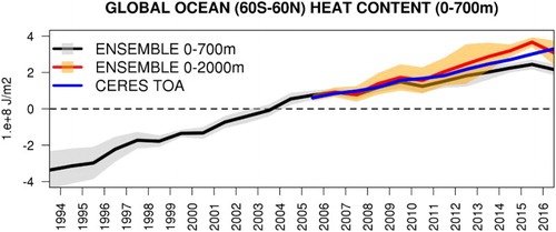
Figure 2.1.2. Basin average from multi-ensemble means of ocean heat content anomalies relative to the 1993–2014 reference mean and integrated over the upper 700 m depth layer for (a) the Mediterranean Sea (product no. 2.1.1 (4 global reanalyses), 2.1.2 (observations); regional reanalyses: 2.1.4–2.1.5), (b) the Iberian-Biscay-Irish area (product no. 2.1.1 (4 global reanalyses), 2.1.2 (observations); regional reanalysis: 2.1.6); (c) the North-West-Shelf (2.1.1 (4 global reanalyses), 2.1.2, observations) and (d) the Arctic area (2.1.1 (4 global reanalyses), 2.1.2 (observations); regional reanalysis: 2.1.7). Shaded areas represent the ensemble spread (ensemble standard deviation) of the products, respectively.

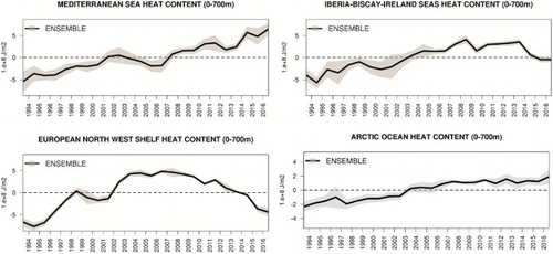
Figure 2.1.3. Regional trends over the period 1993–2016 of ocean heat content (0–700 m) anomalies relative to the 1993–2014 reference period based on the multi-product approach (product no. 2.1.1 (4 global reanalyses), 2.1.2–2.1.3 (observations)). Black dots indicate areas where the signal (ensemble mean of reanalysis trend) exceeds noise (ensemble standard deviation of reanalysis trends), indicating areas of most robust signatures from the multi-product approach.

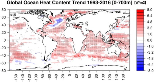
Figure 2.1.4. Regional annual mean ocean heat content anomalies during 2016 relative to the 1993–2014 reference field based on the multi-product approach (product no. 2.1.1 (4 global reanalyses), 2.1.2–2.1.3 (observations)). Black dots indicate areas where the signal (ensemble mean of reanalysis trend) exceeds noise (ensemble standard deviation of reanalysis trends), indicating areas of most robust signatures from the multi-product approach.

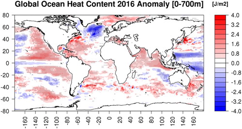
Figure 2.2.1. Near-global (60°S–60°N) averages over the period 2005–2016 of total steric (black), thermosteric (red) and halosteric (green) sea level anomalies relative to the 2005–2016 reference field and integrated over the upper 2000 m depth as derived from the multi-product approach (product no. 2.1.1 (4 global reanalyses) and 2.1.2–2.1.3, observation based). Shaded areas show the ensemble spread (standard deviation). An indirect full depth steric sea level estimate (blue) is obtained from the difference between total sea level from altimetry (see Section 1.5, product no. 2.2.4, 60°S–60°N average) and sea level related to ocean mass changes from gravimetry (product no. 2.2.5).

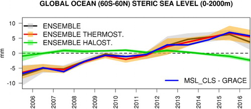
Figure 2.2.2. Regional trend estimates over the period 2005–2016 of (a) total, (b) thermosteric and (c) halosteric sea level integrated over the upper 2000 m depth and derived from the multi-product approach (product no. 2.1.1 (4 global reanalyses) and 2.1.2–2.1.3, observation based). Black dots indicate areas where the signal (ensemble mean of trends) exceeds noise (ensemble standard deviation of trends), indicating areas of most robust signatures from the multi-product approach.

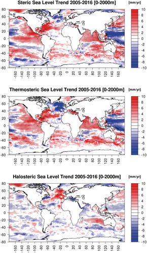
Figure 2.2.3. Regional sea level anomalies integrated over the upper 2000 m depth during 2016 relative to the 2005–2016 reference field of (a) total, (b) thermosteric and (c) halosteric sea level integrated over the upper 2000 m depth and derived from the multi-product approach (product no. 2.1.1 (4 global reanalyses) and 2.1.2–2.1.3, observation based). Black dots indicate areas where the signal (ensemble mean of trends) exceeds noise (ensemble standard deviation of trends), indicating areas of most robust signatures from the multi-product approach.

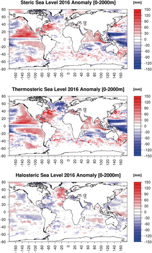
Figure 2.3.1. Volume transport (units SV) from the multi-product approach (product no. 2.3.1) averaged over the period 1993–2014 and and the 2016 year (both red). Estimates of Lumpkin and Speer (2007) have been added for comparison (blue). Uncertainty ranges are derived from the ensemble standard deviation. Arrows indicate the direction of the mean flow through the sections.

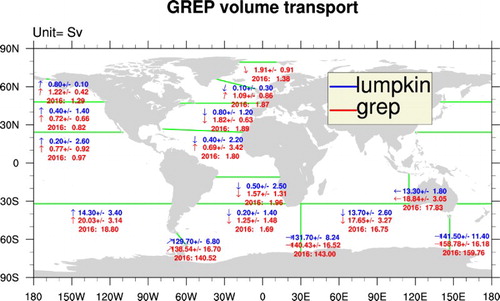
Figure 2.3.2. Monthly time series of volume transport (left panel) and heat transport (right panel) from multi-product approach (product no. 2.3.1) through the Indonesian Throughflow section for 1993–2016 period with a 13-month running mean (top panel) and for 2014–2016 period with a 3-month running mean (bottom panel) (black). The blue shaded area indicates the standard deviation from the ensemble reanalysis. The blue curve shows the SOI (see http://www.cpc.ncep.noaa.gov/data/indices/soi).

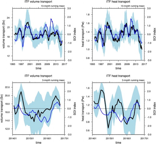
Figure 2.3.3. Total meridional heat transport for the global ocean (a), Atlantic Ocean (b) and Indian plus Pacific Ocean (c) and Indian Ocean (d) from the global reanalysis (product no. 2.3.2) in red and the twin experiment without data assimilation in blue. The solid line is for the reference period 1993–2014 and the dashed line for 2016. The shaded area indicates the standard deviation from 1993–2014 period. Estimates from Lumpkin and Speer (2007) and Ganachaud and Wunsch (2003) are also given with orange vertical bars.

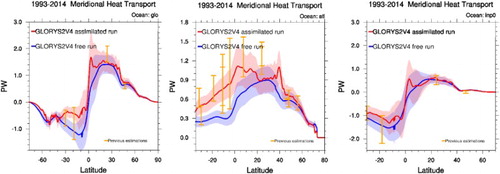
Figure 2.3.4. 2016 anomaly of meridional heat transport in comparison to reference period 1993–2014 for the global ocean (a), the Atlantic ocean (b) and the Indian plus Pacific oceans (c). The red line is the anomaly computed with the global reanalysis (product 2.3.2) and the blue line the twin experiment without data assimilation

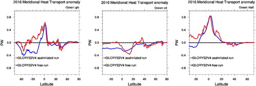
Figure 2.4.1. (a) Annual mean dissolved oxygen (µmol/kg) at the oxygen minimum. (b) Depth (m) of the oxygen minimum within the Oxygen Minimum Zones (O₂ < 90 µmol/kg). (c) Thickness of the layer with O₂< 90 µmol/kg. Contours indicate the oxygen minimum at 4.5, 20, 45, 60 and 90 µmol/kg. Data come from the Global Ocean Biogeochemistry Hindcast from the Copernicus Marine Environment Monitoring Service: product reference 2.4.1 (mean over the period 1993–2014).

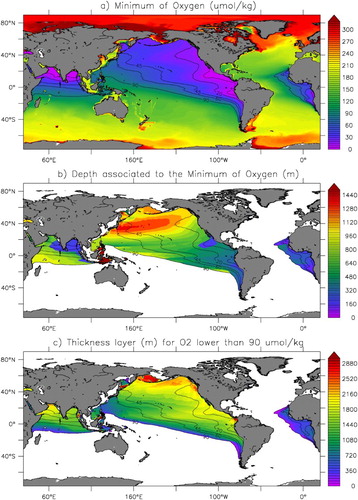
Figure 2.5.1. Time series of monthly average gyre area anomalies for: top left panel: the North Atlantic; top right panel: the South Atlantic; bottom left panel: the North Pacific and bottom right panel: the South Pacific gyres. Data for September 1997 to December 2016, from monthly OC-CCI chlorophyll data (product no. 2.5.1). The value of 0.15 mg/m³ Chl was used as the threshold for defining the gyres in the Atlantic Ocean, according to Aiken et al. (2016); and 0.07 mg/m³ was used for the Pacific gyres, following Polovina et al. (2008). The black lines show the monthly area anomalies of the gyres and the seasonal oscillations in the areas. Blue lines: slopes fitted to data from 2006 or earlier (for comparison with the results of Polovina et al. (2008)), and for the remaining years (2007–2016). Green line: slope fitted to the data for the entire study period.

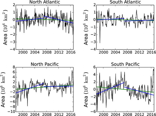
Figure 2.6.1. (upper panel) Monthly sea surface temperature anomaly, from the 1993–2014 climatology, area-averaged over the Niño box 3.4 (black box in b and c) from the multi-product approach (product no. 2.6.1). (lower panels) Temperature (shading, in °C) and winds (arrows, in m/s) anomalies, from the 1993–2014 climatology, time-averaged for the periods (b) January–March 2016 and (c) October–December 2016 (products reference 2.6.1, 2.6.2). The standard deviation of the sea surface temperature from the four multi-product members in the Niño box 3.4 is 0.025°C.

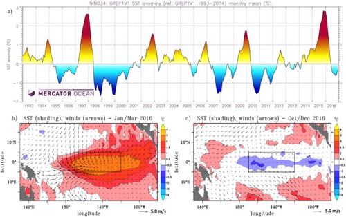
Figure 2.6.2. 0–2000 m steric height anomalies, from the 1993–2014 climatology, along the equatorial Pacific (2°S–2°N) for the periods (a) 2015–2016 and (b) 1997–1998 from the multi-product approach (product no. 2.6.1). For the two periods, the zonally averaged standard deviation of the 0–2000 m steric height anomalies from the four multi-product members is less than 1 cm. Units are cm.

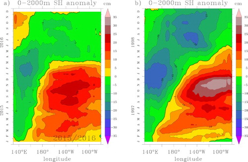
Figure 2.6.3. Temperature anomalies, from the 1993–2014 annual mean, area-averaged in the Niño box 3.4 from the multi-product approach (product no. 2.6.1). The thick black line indicates the position of the isopycnal 1025 kg/m³ and the dashed black line indicates its climatological position. The standard deviation of temperature anomalies from the four multi-product members is less than 0.6°C. Units are °C.

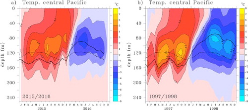
Figure 2.6.4. Mean regional (Niño box 3.4) monthly chlorophyll anomaly relative to the 1998–2014 climatology using OC-CCI v3.1 monthly chlorophyll data as inputs (black, product no. 2.6.3), in blue: Multivariate ENSO Index, see Wolter and Timlin 2011).

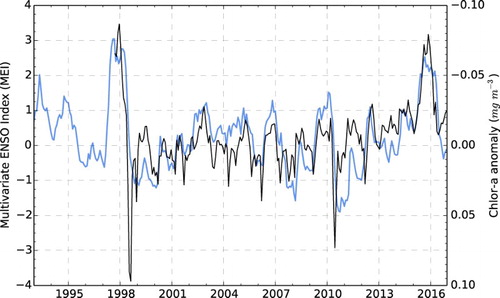
Figure 2.7.1. Upper panel: map of 1993–2016 24-year Sea Surface Temperature trend in (°C per 24 years), from the ensemble mean of the multi-reanalyses CMEMS product reference 2.7.1. Lower panel: time evolution of SST anomalies (°C) computed with CMEMS product reference 2.7.1 with respect to a 1993–2014 climatology from the same product, on global average (black line), and in the black rectangles as shown on the upper panel (coloured lines).

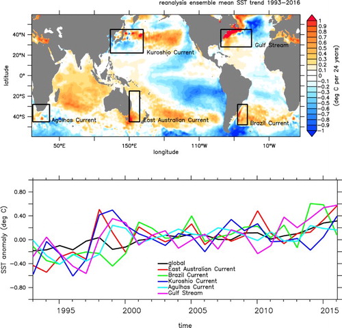
Figure 2.7.2. On the left: vertical sections of eastward velocity 1993–2016 24-year cumulated trends (cm/s per 24 years, colour shading) and mean position of the averaged eastward flow (contours), both zonally averaged across the extensions of the western boundary currents, and computed from GREP ensemble mean (product reference 2.7.1). On the right: eastward current (cm/s) in 1993–2014 (black line) and in 2016 (red line), both zonally averaged and vertically averaged over the 0–500 m layer; standard deviation in between GREP individual yearly estimates for 1993–2014 (grey shading) and for 2016 (red error bars). Zonal averages in the Kuroshio extension are computed from 145°E to 180°E, and in the Gulf Stream extension from 65°W to 40°W.

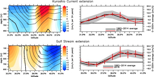
Figure 2.7.3. As in Figure 2.7.2, with zonal averages in the East Australian Current computed from 145°E to 160°E, in the Agulhas current from 21.25°E to 40°E, and in the Brazil Current extension from 54°W to 40°W.

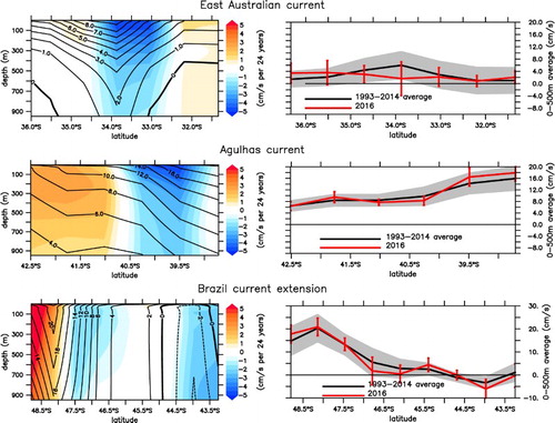
Figure 2.7.4. Colour shading:1993–2016 24-year cumulated trends (cm/s) of currents velocity at 15 m for Northern Hemisphere western boundary currents, computed from the ensemble mean of GREP-V1 reanalyses (product reference 2.7.1) and GLOBCURRENT ESA product (1993–2015) + product reference 2.7.2 15 m geostrophic currents (adding an ageostrophic Ekman component) for year 2016. Cells where the sign of the trend agrees in between all five individual members are indicated with black dots. Contours: mean current velocity for 1993–2014 from the five members ensemble mean (cm/s).

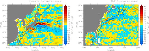
Figure 2.7.5. as Figure 2.7.4 for Southern Hemisphere western boundary currents.

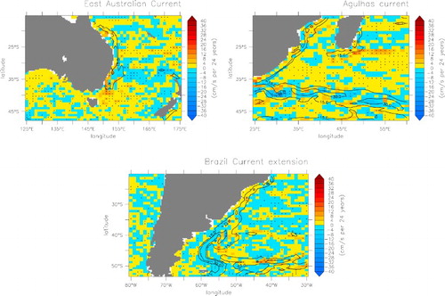
Figure 2.7.6. Standardised EKE over the Kuroshio region (following Bessières et al. 2013) computed with product reference 2.7.3. Blue shaded areas correspond to elongated states (1993–1994, 2002–2004 and 2010–2011), while orange shaded areas fit contracted states periods (1997–2001 and 2009).

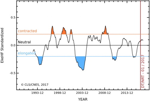
Figure 2.7.7. Courtesy of Bessières et al. (2013). High-frequency EKE (cm²/s²) average for 1997 (top: contracted state) and 2003 (bottom: elongated state). The black line shows the box where the indicator is computed, by averaging this EKE.

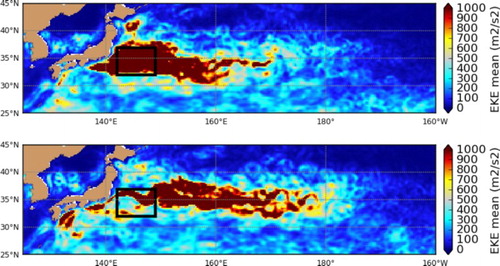
Figure 2.8.1. AMOC strength at 26°N measured by the RAPID array (Smeed et al. 2017) in red and as measured by the GREP (product reference 2.8.1, black with grey shading showing 2 times the standard deviation across the reanalysis products). Top panel: monthly mean values. Bottom panel: monthly mean values with a 12-month running mean. The circulation strength is calculated as the maximum in depth of the circulation profile at each month (see caption for Figure 2.8.2).

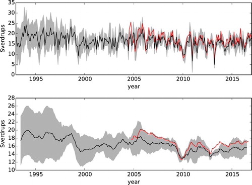
Figure 2.8.2. The time mean AMOC profile at 26°N (average of monthly value from April 2004–March 2015) from the RAPID array (Smeed et al. 2017, red) and from the GREP (product reference 2.8.1, black with grey shading showing 2 times the standard deviation across the reanalysis products). Profiles are calculated as the cumulative total (in depth) of the northwards volume transport.

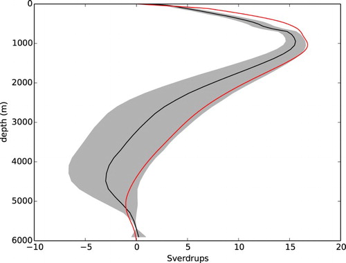
Figure 2.9.1. (a) North Atlantic temperature anomaly averaged over the upper 700 m depth for the year (A) 2016, (B) 2006 and (C) 1994 compared to the reference period 1993–2014 in °C. The anomaly is calculated as an ensemble mean of four global ocean reanalyses (product reference 2.9.1). The northern box indicates the region separated by the Davis Strait, Fram, Strait and 47°N named hereafter the subpolar gyre box and the southern box indicates the region separated between 47°N and the RAPID line at 26°N.

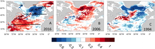
Figure 2.9.2. Depth-time plot of the ensemble mean (product reference 2.9.1) temperature (A) and salinity (B) anomaly (relative to 1993–2014) averaged over subpolar gyre box indicated in Figure 2.9.1. Black dots show areas where the signal exceeds the noise indicating the robustness of the anomalous pattern. (C) Annual mean vertical temperature anomaly (rel. to the 1993–2014 period) profile for the year 2016 (in orange), for 2015 (in blue), for 2006 (in yellow), for 1994 (in green) and variability over the period (in grey) (right).

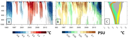
Figure 2.9.3. (a) North Atlantic Oscillation (NAO) index (Hurrel 1995, product reference 2.9.3), (b) Net surface anomaly flux over the North Atlantic region (rel. to the 1993–2014 period) averaged over the subpolar gyre box area shown in Figure 2.9.1 using the ERA-Interim product (product reference 2.9.2). (c) Ocean heat content anomaly (rel. to the 1993–2014 period) integrated over the upper 700 m depth and based on the product reference 2.9.1 in red in the subpolar gyre region and in blue between 26°N and 47°N.

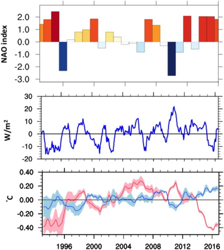
Figure 2.9.4. Maximum mixed layer (in metres) over the period 1993–2016, using the GLORYS2V4 reanalysis (distributed in product reference 2.9.1). In contour, the three main convection regions: Labrador, Cape Farewell, Irminger.

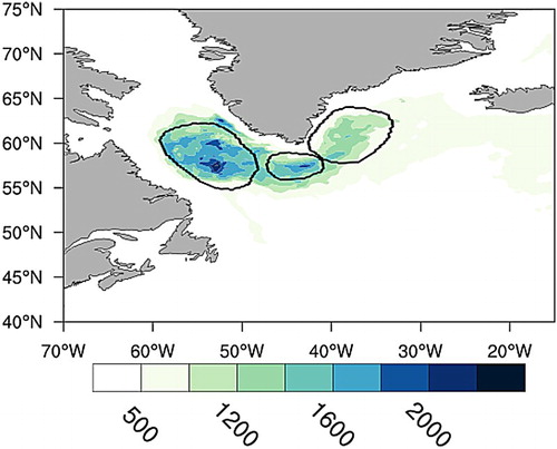
Figure 2.9.5. Anomalies of mixed layer depth compared to the reference period 1993–2014, in red: ensembles mean and in grey 1 standard deviation for (A) the Labrador sea region, (B) the Cape Farewell region and (C) the Irminger Sea. Product reference 2.9.1.

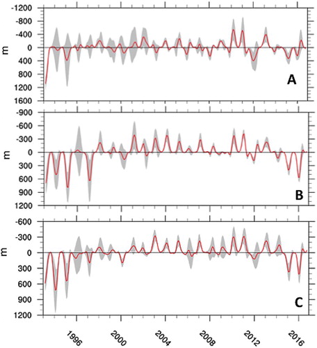
Figure 2.10.1. Mean 1993–2016 FW content (units in metres) for the ensemble mean global reanalysis product (GREP) (a) and the standard deviation among the four members of the GREP ensemble (b). Products no. 2.10.1.

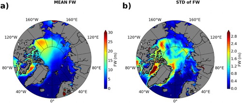
Figure 2.10.2. 1993–2016 time series of monthly anomalies (mean seasonal cycle removed) of freshwater content (red) and sea ice volume (black, see also Section 1.7) anomalies relative to the 1993–2016 climatology for the ensemble mean global reanalysis product (GREP). The spatial domain corresponds to the Arctic Ocean basins with a water depth greater than 500 m (definition of Rabe et al. (2014). The uncertainty (shaded areas) is the standard deviation among the four members of the GREP ensemble. Products no. 2.10.1.

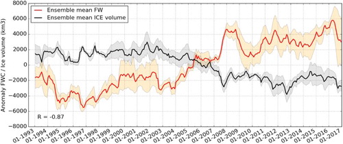
Figure 2.10.3. FW content anomaly of 2016 from the 1993–2016 from the 1993–2016 FW content climatology (units in metres). Product no. 2.10.1 (GREP).

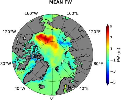
The 2016 record allows a comparison of the oceanic conditions in the tropical Pacific during the 2015–2016 period with regard to the 1997–1998 period. Figure 2.6.2 shows the 0–2000 m steric height anomaly for the two periods, and basin-wide variations clearly appear, dominated by a large-scale zonal seesaw centred on the dateline, with positive anomalies mostly observed in the central-eastern Pacific during 2015 (up to 25 cm at 130°W in November) and negative anomalies during 2016 (down to 10 cm in May). Even if these central-eastern Pacific characteristics are stronger than ENSO composites (Gasparin and Roemmich 2017), they remain significantly lower than that of the 1997/1998 event (Xue and Kumar 2017), which peaks at 35 cm at 110°W in November 1997 and −20 cm at 150°W in June 1998. These variations reflect upward and downward deflections of the thermocline, respectively associated with negative and positive steric height anomaly as shown below, and result from surface wind variations at interannual timescales (Gasparin and Roemmich 2017). Superimposed on these basin-wide variations, eastward propagating anomalies mark the presence of intraseasonal Kelvin waves, which have been identified as one of the key factors for the onset of El Niño (e.g. Kessler et al. 1995), but note that the monthly temperature estimates limit the representation of these timescales.

To further investigate upper ocean conditions, temperature anomaly area-averaged between 170°W and 120°W along the equator is shown in the upper 300 m in Figure 2.6.3. Positive anomalies during August–October 2015 (>4°C) are linked to a downward deflection of 20 m of the thermocline, while in October 1997 a 30 m-downward deflection caused a stronger anomaly (>6°C). Compared to 1998, the negative anomaly in April–May 2016 is much lower with an upward deflection of 30 m of the thermocline (60 m in June–November 1998). Interannual variations are also observed in chlorophyll concentrations. In Figure 2.6.4, the chlorophyll anomaly in the Niño3.4 box closely follows the oscillations in the Multivariate ENSO Index for the entire time series. The two prominent El Niño events in 1997–1998 and 2015–2016 correspond to strong negative anomalies in chlorophyll concentration. This is consistent with the high positive anomalies for these periods in the sea surface temperature: the increased stability and associated decrease in upwelling would reduce the supply of nutrients to the surface and hence the concentration of phytoplankton (Radenac et al. 2012). Xue and Kumar (2017) further discuss the characteristics of the 2015/2016 and 1997/1998 El Niños. They highlight that the various flavours of ENSO lead to different long-distance effects such as along the Californian coast, where impacts on subsurface temperature anomalies were much weaker during the 2015/2016 El Niño than during the 1997/1998 El Niño (Jacox et al. 2016).

Finally, the 2015/2016 was likely the most widely anticipated and documented ENSO event ever, resulting from almost four decades of advancements in observing and prediction systems (L’Heureux et al. 2017). However, seasonal forecasts of El Niño occurrence and amplitude remain a major research challenge as shown by the case of the year 2014. Despite the presence of oceanic and atmospheric indicators in early 2014 – apparently signalling the onset of a strong El Niño – El Niño never materialised that year (Hu and Federov 2016; Corbett et al. 2017). The ongoing development of the deep ocean observing system (Johnson et al. 2015), and the evolution of its upper part (Legler et al. 2015), will improve the scale-matching of in situ and remote observations. In particular, the description and understanding of salinity-related processes and their implication in ENSO evolution are still challenging, and many studies have recently shown that including salinity in forecasting systems is essential to correctly forecast ENSO (e.g. Hackert et al. 2014; Zhu et al. 2014; Shi et al. 2015). Thus, providing an accurate full picture of the ocean is crucial for near-real time monitoring of El Niño-related processes, and further improvement for ENSO forecast activities.

2.7. Western boundary currents

Leading authors: Marie Drévillon, Jean-François Legeais.

Contributing authors: Andrea Storto, K. Andrew Peterson, Hao Zuo, Marie-Hélène Rio, Yann Drillet, Eric Greiner.

Statement of outcome: The western boundary currents experience a warming trend over the period 1993–2016. Concurrent with this warming, most of the western boundary currents seem to shift poleward. The poleward shift of the Kuroshio is very strong in 2016, which could be linked to the 2015/2016 El Nino. This signal may also be the signature of the contracted mode of the Kuroshio, as measured by the eddy kinetic energy (EKE) index. The Gulf Stream experiences an equatorward shift, which is well marked in 2016, and which may be linked with the cold temperature anomaly that can be diagnosed in the North Atlantic.

Products used:

Table

Ref. No.	Product name & type	Documentation
2.7.1	GLOBAL_REANALYSIS_PHY_001_026 Reanalysis	QUID: http://marine.copernicus.eu/documents/QUID/CMEMS-GLO-QUID-001-026.pdf PUM: http://marine.copernicus.eu/documents/PUM/CMEMS-GLO-PUM-001-026.pdf
2.7.2	GLOBAL_ANALYSIS_PHYS_001_020 In situ, remote sensing	QUID: http://marine.copernicus.eu/documents/QUID/CMEMS-GLO-QUID-001-020.pdf PUM : http://marine.copernicus.eu/documents/PUM/CMEMS-GLO-PUM-001-020.pdf
2.7.3	SEALEVEL_GLO_PHY_L4_REP_OBSERVATIONS_008_047 Remote sensing	QUID: http://marine.copernicus.eu/documents/QUID/CMEMS-SL-QUID-008-032-051.pdf PUM: http://marine.copernicus.eu/documents/PUM/CMEMS-SL-PUM-008-032-051.pdf

Strong poleward Western Boundary Currents are present in the world’s major ocean basins, which compensate for the wind-driven equatorward transport in the ocean subtropical gyres (Imawaki et al., 2013). The Kuroshio in the North Pacific Ocean, the Gulf Stream in the North Atlantic, the Agulhas Current in the Indian Ocean can be distinguished on Figure 1.6.1 of Section 1.6, where 1993–2014 climatological velocity reach more than 1 m/s In the East Australian Current in the South Pacific, and the Brazil Current in the South Atlantic, climatological velocities are of the order of 50 cm/s.

The EKE levels are elevated in the western boundary currents, and part of their interannual variability comes from large eddies or meanders, as shown for instance by sea level anomaly variances (Ducet et al. 2000). The eddies play an important role in the position of the WBC, as well as in the interaction with the atmosphere (Ma et al. 2016). At interannual to decadal timescale, western boundary currents respond to ‘regime shifts’ related to climate variability modes such as for instance the North Atlantic Oscillation for the Gulf Stream (Watelet et al. 2017) or the Pacific Decadal Oscillation for the Kuroshio, also impacting the ocean ecosystems (Overland et al. 2008). Last but not least, the western boundary currents variability can be related to low frequency variability of the climate system and long-term redistribution of heat in the climate system. Wu et al. (2012) and Yang et al. (2016) show that global warming trends are locally enhanced in Western Boundary Currents, and that a poleward shift of most western boundary currents is expected from climate scenarios’ results. The Gulf Stream is expected to be weaker under global warming, likely related to a weakening of the AMOC.

In the following, we will focus on interannual to decadal time scale changes in the western boundary currents over the 1993–2016 period, with a specific focus on the EKE of the Kuroshio (Bessières et al. 2013). As shown in Figure 2.7.1, and consistent with Wu et al. (2012) and Yang et al. (2016, Fig. 2), the increase in time of the average western boundary currents sea-surface-temperature over the last 24 years (1993–2016), as seen by CMEMS product reference 2.7.1, was at least that of the global average on the same period, which is around 0.25°C per 24 years (slope of the linear trend on global average, see also Section 1.1 and Figure 1.1.1). Yang et al. (2016) also noted, that western boundary currents undergo strong interannual to decadal variability, and consequently that low frequency changes in the western boundary currents that can be monitored here over a 24-year period will have to be confirmed with longer time series.

The Global Reanalysis Ensemble Product GREP ensemble mean, CMEMS product reference 2.7.1, was used to derive mean vertical sections of eastward current in the western boundary current extensions, and to compute the 1993–2014 trend of eastward current in the same area, following Wu et al. (2012). The zonally and vertically averaged eastward flow is shown with error bars, derived from the standard deviation in between GREP individual members’ yearly estimates. Figure 2.7.2 suggests that the Kuroshio Current extension experienced a poleward shift during the last 24 years, which was well marked in 2016. The change in 2016 is particularly significant near 35°N in the Kuroshio, as part the 2016 mean 0–500 m eastward current estimate is outside of the climatological envelope. This result is in agreement with the twentieth century trend in the Kuroshio as depicted in Wu et al. (2012, their Fig. 2) and based on SODA (1900–2008). On the contrary in Figure 2.7.2, the Gulf Stream experienced a deceleration or a southward shift during the recent 24-years period, which is different from the poleward shift of the Gulf Stream during the twentieth century as depicted by Wu et al. (2012). The southward shift is also well marked in 2016 compared to the average period 1993–2014.

In the Southern Hemisphere in Figure 2.7.3, a poleward shift is observed in the Agulhas and Brazil current over the time period 1993–2016, and the mean position of those currents is located poleward of the position of the same currents in SODA (Wu et al. 2012). The East Australian Current 24-year trend captured by CMEMS product reference 2.7.1 is a mean deceleration which is different from the acceleration captured by SODA in the twentieth century in Wu et al (2012). Of course, interannual variability of the ocean influences the position and intensity of Western Boundary Currents in 2016, as captured in Figures 2.7.2 and 2.7.3. The El Nino 2015/2016 may have enhanced the poleward migrations of the Kuroshio and East Australian currents in 2016 in the Pacific (see Section 2.6). This is also suggested by the positive sea surface temperature anomalies of in the Kuroshio and East Australian Current as shown in Figure 2.7.1 in 2015 and 2016. The surface temperature anomaly was also strongly positive in 1997 and 1998 during the most intense El Nino event of the period. Finally, the cold anomaly in the North Atlantic (see Section 2.9) may have played a role in the equatorward migration of the Gulf Stream in 2016.

Focussing on trends of near surface (around 15 m depth) current velocity, computed with a larger five-member ensemble mean composed of GREP (four global ocean reanalyses) plus ESA Globcurrent products for the 1993–2015 period. Note that in 2016, ESA Globcurrent time series is complemented with CMEMS product reference 2.7.2, plus an ageostrophic current component computed from an Ekman model (Larnicol et al. 2006). CMEMS product reference 2.7.2 is based on satellite altimetry observations which are also assimilated by the reanalyses. Trends computed here thus strongly rely on satellite altimetry observations, each ocean reanalysis (or Globcurrent) performing its own compromise in between all sources of information, including the atmospheric forcing (ERA-Interim atmospheric reanalysis) and the other observations assimilated by the ocean reanalyses. Following the trends shown in Figure 2.7.4, the near surface Gulf Stream decelerated or shifted to the south during the 24-year period, by 5 to 10 cm/s in the Gulf Stream extension. The Kuroshio was shifted approximately one degree north of its average 1993–2014 position as also seen in Figure 2.7.2, and with a change of 10–15 cm/s east of 150°E, consistently with the trends for the whole water column displayed in Figure 2.7.2. In the Southern Hemisphere Figure 2.7.5, the large-scale patterns of the trends are quite consistent with that of another ensemble of reanalyses (SODA, ORAS-4, GECCO and GECCO2) for the period 1958–2001 for the 0–100 m average current velocity (Yang et al. 2016, their Fig. 5) with values reaching locally 20 cm/s per century (equivalent to 5 cm/s per 24 years). The Malvinas current decelerated while the Malvinas return branch accelerated which is in better agreement with the trends computed from CMIP/RCP45 experiments for the period 2006–2100 (Yang et al 2015, their Fig. 8). Also consistent with projections for the period 2006–2100 the Agulhas return branch decelerated, or possibly shifted South, and the Tasman Front current decelerated.

Again, these results will have to be confirmed on the longer term, but they underline significant variability and long-term changes in the ocean western boundary currents over the first thousand metres, and stress the need for a sustainable observing and monitoring system for the world’s oceans which would improve the monitoring and uncertainty assessment of this changes, and of the related changes in integrated transports (Section 2.3).

2.7.1. The Kuroshio Ocean State Indicator

The long-term mean and trends alone do not give a complete view of the likely changes in position of unstable western boundary current extensions. In the following, we thus present an indicator based on monthly EKE estimates.

The Kuroshio Extension is an eastward-flowing current in the subtropical western North Pacific after the Kuroshio separates from the coast of Japan at 35°N, 140°E. Being the extension of a wind-driven western boundary current, the Kuroshio Extension is characterised by a strong variability and is rich in large-amplitude meanders and energetic eddies. The Kuroshio Extension region has the largest sea surface height variability on sub-annual and decadal time scales in the extratropical North Pacific Ocean. Prediction and monitoring of the path of the Kuroshio are of huge importance for local economies as the position of the Kuroshio extension strongly determines the regions where phytoplankton and hence fish are located.

Two rather different states of the Kuroshio extension are observed: an ‘elongated state’ (also called ‘strong state’) corresponding to a narrow strong steady jet, and a ‘contracted state’ (also called ‘weak state’) in which the jet is weaker and more unsteady, spreading on a wider latitudinal band. When the Kuroshio Extension jet is in a contracted (elongated) state, the upstream Kuroshio Extension path tends to become more (less) variable and regional EKE level tends to be higher (lower). Bessières et al. (2013) show that, to monitor both those states, an average of EKE derived from the observed altimeter sea surface heights over a box located between 142–149°E and 32–37°N is a good indicator of Kuroshio extension variations.

In Figure 2.7.6, the EKE index computed following Bessières et al. (2013) from product reference 3 is shown, and blue shaded areas correspond to elongated states periods (1994, 2002–2004, 2010–2011 and 2015), while orange shaded areas fit contracted states periods (1997–2001 and 2008–2009). Examples of these two opposite phases are illustrated with years 1997 and 2003 in Figure 2.7.7. In between these two opposite phases, the Kuroshio Extension jet has many intermediate states of transition and presents either progressively weakening (1994–1997 and 2004–2009) or strengthening (2001–2002 and 2009–2010) trends. In 2016, the indicator reveals an intermediate neutral but strengthening phase.

2.8. Atlantic Meridional Overturning Circulation

Leading authors: Laura Jackson, Clotilde Dubois.

Contributing authors: Simona Masina, Andrea Storto, Hao Zuo.

Statement of main outcome: The AMOC shows considerable variability on monthly and interannual timescales. There has also been a weakening over the last decade. However, this may be due to longer term variability rather than an ongoing trend.

Products used:

Table

Ref. No.	Product name & type	Documentation
2.8.1	GLOBAL_REANALYSIS_PHY_001_026 Reanalysis	QUID: http://marine.copernicus.eu/documents/QUID/CMEMS-GLO-QUID-001-026.pdf PUM: http://marine.copernicus.eu/documents/PUM/CMEMS-GLO-PUM-001-026.pdf

The AMOC is an important part of the climate system which transports warm and salty waters northwards in the Atlantic, and hence both natural variability and forced changes of the circulation strength can drive changes in Atlantic sea temperatures (Ba et al. 2014; Jackson et al. 2015). Climate models show projections of AMOC weakening over the next century due to anthropogenic climate change, although there are significant uncertainties as to the magnitude of the change (Collins et al. 2013).

The AMOC has been measured with the RAPID array at 26°N since April 2004 (Smeed et al. 2017). Over this period the mean strength is 16.9 Sv in the observations and 15.6 ± 1.6 Sv in the GREP (product reference 2.8.1, uncertainty is 2 times the standard deviation of the ensemble values). The variability of the GREP time series of AMOC strength (Figure 2.8.1) agrees well with the time series observed from the RAPID array, although the circulation strength of the GREP is generally weaker than in the observations. There is considerable monthly variability and the monthly mean values are correlated with a value of 0.82 over the observational period. Profiles of the AMOC at 26°N (Figure 2.8.2) show too little northwards transport in the upper 800 m in the GREP. There is also a lot of uncertainty in the GREP below 2000 m, with three out of the four reanalyses contributing to the GREP having too shallow a circulation.

One feature of the AMOC time series is the weak strength in winter 2009–2010 (McCarthy et al. 2012) which appears to be driven by atmospheric forcing (Roberts et al. 2013; Zhao and Johns 2014). This resulted in cooling of the upper North Atlantic north of the RAPID array and warming south of the array in 2010 (see Figure 2.9.2; Cunningham et al. 2013; Bryden et al. 2014).

There are also multiannual to decadal changes seen in the AMOC strength. The GREP shows significant uncertainty before 2001 followed by an increase from 2001–2006 (trend = 0.48 Sv/year, p = .04) and then a decrease from 2005–2012 (trend = −0.53 Sverdrups/year, p = .04). This latter trend was also seen in the observations (trend = −0.67 Sverdrups/year, p = .03) and has been linked to reductions in density in the Labrador Sea and reduction in deep convection there (Figure 2.9.5; Robson et al. 2014). Since 2012 the AMOC strength has largely been stable (no significant trend in either the observations or the GREP).

Jackson et al. (2016) suggested that the observed trend from 2005–2012 is part of multidecadal variability rather than an ongoing trend, which is supported by these results. Robson et al. (2016) showed that there has been a cooling of the upper subpolar North Atlantic since 2005 and that this is consistent with a weakening northwards heat transport. This has potentially contributed to the recent cold anomaly seen in the subpolar gyre in 2016 (Section 2.9), although the main cause of this cold anomaly is thought to be surface fluxes (Josey et al. 2017).

2.9. Changes in the North Atlantic

Leading authors: Clotilde Dubois, Karina von Schuckmann, Simon Josey.

Contributing author: Adrien Ceschin.

Statement of outcome: The North Atlantic has experienced a strong and deep (>500 m) cooling and freshening in the subpolar gyre region since 2014. Such cooling is related to the North Atlantic Oscillation and East Atlantic pattern which generate strong heat lost at the ocean-atmosphere interface. The recent freshening has not been observed during the last 25 years.

Products used:

Table

Ref. No.	Product name & type	Documentation
2.9.1	GLOBAL_REANALYSIS_PHY_001_026 Reanalysis	PUM: http://marine.copernicus.eu/documents/PUM/CMEMS-GLO-PUM-001-026.pdf QUID: http://marine.copernicus.eu/documents/QUID/CMEMS-GLO-QUID-001-026.pdf
2.9.2	ERA-Interim Reanalysis (atmosphere)	https://www.ecmwf.int/en/research/climate-reanalysis/era-interim Dee (2011)
2.9.3	North Atlantic Oscillation index Climate indicator based on reanalysis (atmosphere)	https://crudata.uea.ac.uk/cru/data/nao/ Hurrell (1995)

Since 2014, extreme cold sub-surface anomalies have been observed spanning the subpolar North Atlantic waters, this region is named here after ‘subpolar gyre’, and these have persisted up to the year 2016 (Figures 2.9.1 and 2.9.2). The cold ocean temperatures are particularly noticeable as there has been a general increase of temperatures, ocean heat content and sea level elsewhere around the globe (Sections 1.1, 1.2, 1.5, 2.1, 2.2). The multi-product ocean reanalysis (product no. 2.9.1) is used here to analyse the interannual and decadal variability in the North Atlantic area over the period 1993–2016.

These cold and fresh anomalies are located in an ocean area of particular importance (Figure 2.9.2). Ocean changes in this region are driven by several processes: (1) the physical interactions at the atmosphere–ocean interface controlling heat and momentum transfer; (2) the internal ocean dynamic processes such as the AMOC controlling the global ocean climate at decadal and longer time scales; (3) the wind-driven circulation changes of the major ocean gyre systems and (4) the formation of new water masses connecting the two through its exchange mechanisms between the surface and deep ocean and ventilating and renewing water layers of the interior ocean.

As observed for regional sea level and regional ocean heat content (Sections 2.1 and 2.2), a meridional dipole pattern prevails in the North Atlantic area during 2016 with anomalous low upper ocean temperature in the subpolar North Atlantic, and anomalous high values in the subtropical region (Figure 2.9.1(A)). A view into the interior of the ocean shows that these patterns extend down to more than 700 m depth, in particular in the subpolar North Atlantic (Figure 2.9.2, see also Section 1.2). Moreover, this meridional dipole pattern is persistent since 2014 (see also Figure 2.9.3(C)), i.e. when the North Atlantic Oscillation entered a strong positive phase (Figure 2.9.3(A)). During 2015 – i.e. when the so-called ‘cold blob event’ strengthened – the signature is surface intensified and appears to propagate downwards afterwards (Figure 2.9.2(C)).

Although less pronounced, events of concurrent and deep reaching negative temperature anomalies in the subpolar North Atlantic and positive temperature anomalies in the subtropical area occur also at the beginning of the time series, i.e. during the 1993–1995 period (Figures 2.9.2 and 2.9.3(C)). Cold anomalies prevail in the upper 700 m depth during this period (Figure 2.9.2(A)) and characterise much of the subpolar area (Figure 2.9.1(C)), whereas concurrent positive anomalies in the subpolar region are less pronounced (Figure 2.9.1(C)). Previous studies showed the link between the North Atlantic Oscillation and East Atlantic Pattern indices and temperature anomalies in the subpolar gyre area (Robson et al. 2012; Josey et al. 2017). Since 2014, the North Atlantic Oscillation index is in a strong positive phase (Figure 2.9.3(A)) and the East Atlantic Pattern has also been in an extreme state. Whereas, during the period 2003–2009, North Atlantic Oscillation index was more in a neutral and negative phase, where positive temperature anomalies prevail in the upper 700 m depth of the subpolar North Atlantic (Figure 2.9.2(A)) and re-emerge strongly occurs during the year 2011. Previous studies have shown cold sea surface temperature in the North Atlantic, together with extreme heat loss in the region and North Atlantic Oscillation/ East Atlantic Pattern index extremes (e.g. Josey et al. 2015, 2017).

Also, this area is affected by freshwater inflow from ice melting processes in the Arctic, which in turn induce changes in the North Atlantic density field (Sections 1.4 and 2.10). Concurrent to the emergence of low temperature anomalies, a signature of anomalous low salinity appears (Figure 2.9.2(B)). The interplay of these different physical ocean processes in this area have a potential impact on regional and global climate and weather patterns, in particular over the European continent and North America (Marshall et al. 2001; Duchez et al. 2016).

Net surface heat fluxes from the ERA-Interim dataset exhibit anomalous heat loss during the successive winters of 2013/2014 and 2014/2015, followed by a return to near normal heat loss in winter 2015/2016 linked to the North Atlantic Oscillation (Figure 2.9.3(B)). Very similar heat loss variations are found with the NCEP/NCAR product which indicates that these results are not sensitive to the choice of the atmospheric reanalysis system (not shown here). Since those cold winters, the ocean heat content of the upper 700 m in the North Atlantic region has decreased reaching its minimum value of −0.40°C over the period. Thus, the cold anomaly has persisted in 2016 despite winter 2015/2016 heat loss being close to normal. This suggests that one or more winters of anomalously weak heat loss will be necessary before the anomaly starts to significantly diminish. The ocean heat content (Section 2.1) of the sub-polar gyre region has decreased during the last decade (Figure 2.1.3, Häkkinen et al. 2015). This change in local heat storage can in turn affect the winter’s air–sea exchange on ocean and atmospheric transport pathways, as well as regional sea level patterns through thermosteric effects (see Sections 1.4 and 2.2). During the severe winters, the North Atlantic mid- and high-latitude air–sea heat exchange was dominated by anomalously strong north-westerly winds, bringing exceptionally cold and dry air across the north-eastern Atlantic (Grist et al. 2016). In particular, recent studies have identified that this cold pattern is part of interannual to decadal variability through its connection to climate modes such as the East Atlantic Pattern and the North Atlantic Oscillation (Figure 2.9.3(a); Robson et al. 2012; Yeager et al. 2015; Josey et al. 2015), affecting also deeper layers of the North Atlantic (Häkkinen et al. 2015) or part of the multi-decadal variability of the Atlantic Multi-Decadal Oscillation which is moving to a negative phase (Figure 2.9.3(c); McCarthy et al. 2015). Josey et al. (2017) have reviewed the causes and consequences of the Atlantic cold anomaly and find that its primary cause is the extreme heat loss in winters 2013/2014 and 2014/2015.

Due to its location in the middle of the North Atlantic, this cold and fresh anomaly could be related to most intense formation of deep water (Labrador Sea Water, Section 4.3; Kieke and Yashayaev (2015), Yashayaev and Loder (2016, 2017)), and also in the Irminger Sea and Cape Farewell (Piron et al. 2017). In the North Atlantic, the deep convection regions are found in the Labrador, Cape Farewell and Irminger Sea (Figure 2.9.4). Time series of the anomalies of the maximum mixed layer depth show strong deep convection in the 1990s, whereas the 2000s experienced less deep water formation (Figure 2.9.5). An increase in deep convection emerges during the recent years, especially in the Irminger and Cape Farewell regions. Also, other studies suggested that increase in freshwater fluxes from Greenland have also contributed to changes in Labrador Sea Water (Yang et al. 2016), and are linked to AMOC strength (Yeager et al. 2015; Brunnabend et al. 2015; Yang et al. 2016).

However, it suggests that the Atlantic cold event could be linked to Atlantic multi-decadal variability and to the AMOC system on multi-decadal time scales (Jackson et al. 2016). Many studies are now predicting a cooling of the North Atlantic as the Altantic Multi Decadal Oscillation may be entering a prolonged negative phase (Hermanson et al. 2014; Klöwer et al. 2014; Robson et al. 2014, McCarthy et al. 2015). As discussed above, simultaneous changes in atmospheric circulation contributed to this cooling pattern at seasonal to interannual time scales, but it is also suggested that they cannot fully explain the cooling, indicating that ocean circulation changes at decadal time scales are an important forcing factor (Yeager et al. 2015; Robson et al. 2014; Smeed et al. 2014).

2.10. Arctic ocean freshwater content

Leading authors: Gilles Garric, Olga Hernandez.

Contributing authors: Clement Bricaud, Andrea Storto, Kenneth Andrew Peterson, Hao Zuo.

Statement of outcome: The global reanalysis products show a remarkable increase in freshwater content in the Arctic Ocean since the mid 90’s strongly linked to sea ice volume variability. 2016 witnessed the highest freshwater content in the Artic for the last 24 years.

Products used:

Table

Ref. No.	Product name & type	Documentation
2.10.1	GLOBAL_REANALYSIS_PHY_001_026 Reanalysis	PUM: http://marine.copernicus.eu/documents/PUM/CMEMS-GLO-PUM-001-026.pdf QUID: http://marine.copernicus.eu/documents/QUID/CMEMS-GLO-QUID-001-026.pdf

Many studies have already highlighted that one of the main factors controlling the strength and sensitivity of the meridional overturning circulation (AMOC, see Section 2.8) is the cycling of the freshwater at high northern latitudes (e.g. Stouffer et al. 2006, or Carmack et al. (2016) for a recent review). A delicate density balance exists indeed in the deep water formation regions of the North Atlantic (Mauritzen et al. 2012), so that only slight variations in nearby Arctic-North Atlantic freshwater exchanges can influence the large-scale ocean circulation (Mysak et al. 2005; Rahmstorf et al. 2005; Zhang and Vallis 2006). Importance of temperature-salinity compensation in the subpolar North Atlantic region is highlighted in Section 2.2 discussing relative impact of halosteric changes (Figure 2.2(c)). The Arctic climate is undergoing unprecedented and drastic changes, affecting all the components of the Arctic system. Many of these changes affect the hydrological cycle and the freshwater budget of the Arctic region and an increasing literature has been recently published on key emerging issues of the Arctic freshwater budget and its changes (see for instance Prowse et al. 2015a, 2015b; Carmack et al. 2016; Lique et al. 2016). The Arctic Ocean is freshening (Proshutinsky et al. 2009; Rabe et al. 2014; Haine et al. 2015), sea ice is retreating and thinning (see Section 1.7) and exchanges of salt with the bordering subarctic oceans are undergoing substantial changes (Beszczynska-Möller et al. 2011; Woodgate et al. 2012). Freshwater is stored within the Arctic Ocean in the form of relatively fresh ocean waters in the surface layer and sea ice. Observations are particularly sparse in the Polar Regions and modelling systems have been widely used and are a powerful tool to gain understanding on the Arctic freshwater system (Jahn et al. 2012; Lique et al. 2016).

In this section, we present how the ensemble mean global reanalysis products (GREP: GLORYS2V4 from Mercator Ocean (Fr), ORAS5 from ECMWF, FOAM/GloSea from Met Office (UK), and C-GLORS from CMCC (It)) represent the Arctic freshwater variability over the last 25 years and which processes are involved in the equilibrium. We calculate the liquid freshwater content (FW in metres) from the surface to the bottom of the upper ocean per unit area as: $FW={\int }_{\mathrm{bottom}}^0(S\text{ref}-S(z)/S\text{ref) }\text{d}z$, where S is salinity, dz the vertical cell thickness of the dataset and Sref the salinity reference set to 34.8. Waters saltier than the 34.8 reference are not included in the estimation of the freshwater content. This salinity reference corresponds to the mean Arctic salinity according to Aagaard and Carmack (1989) and is widely used in Arctic Freshwater studies (Serreze et al. 2006; Proshutinsky et al. 2009; Condron et al. 2009; Jahn et al. 2012; Haine et al. 2015; Wang et al. 2016). The total freshwater content (FWC in km³) corresponds to the integration of FW over the Arctic domain. The distribution of the liquid FW storage represented by GREP shows, as expected, a clear maximum in the Beaufort Sea region together with a maximum in the Baffin Bay (Figure 2.3.1). With a mean value of 80700 ± 7000 km³ over the 1993–2015 period (calculated in the domain defined by Jahn et al. 2012), the FWC estimated by GREP is in the upper range of FWC simulated by models (53,400–89,700 km³) presented in (Jahn et al. 2012), in the lower range of FWC simulated by the 14 CORE-II (Coordinated Ocean-ice Reference Experiments) models (75,000–137,000 km³) (Wang et al. 2016) and in the upper range of the observations-based estimates from Serreze et al. (2006) (74,000 ± 7400). With almost 9% of uncertainties, the FWC differs among the GREP products but remains in the error bars of the observations and is largely below the range produced by models without assimilation (Jahn et al. 2012; Wang et al. 2016). Although the uncertainties from the GREP ensemble are uniformly spread in the Arctic basin there are two local maxima in the Laptev Sea and in the northern gateway of the Fram Strait. Outside the Arctic Ocean, the Baffin Bay is the location where the greatest spread is observed (Figure 2.10.1).

From Figure 2.3.2, a clear positive and significant (p-value < .01) trend is estimated with the GREP products from 1995 to 2012 of 502 ± 144 km³/yr which is consistent with the observations-based trend of 600 ± 300 km³/yr from Rabe et al. (2014) but on the 1992–2012 period. Despite different initial conditions in 1993 for the GREP members, the GREP products show a decline in the FWC from 1993 to 1995. As already pointed out by Ilicak et al. (2016) in CORE-II experiments, the use of common atmospheric driver, e.g. ERA-Interim in the GREP products, may likely explain remarkable correlation, between the members. Since 2008, the trend is however less pronounced than the previous ten years. During the first half of 2016, the FWC estimated by GREP ensemble mean shows the maximum value ever encountered in the 1993–2015 period (Figure 2.10.2). The year 2016 is characterised by a strong positive anomaly (up to 5 m height) in nearly the entire Canadian Basin (Figure 2.10.3). The second half of 2016 also shows an important decrease of the FW storage along with large uncertainties.

The sea ice volume anomalies (see also Section 1.7) are superimposed in the Figure 2.10.2. An important and significant linear anti-correlation of −0.87 is found between the two time series. A weaker anti-correlation of −0.48, but still significant (p-value < .01), is found with these detrended time series. Water from river runoff, inflow of relatively fresh water from the Pacific through the Bering Strait, and precipitation minus evaporation are net sources of the Arctic Ocean freshwater budget. These are largely balanced by a net export of water to the North Atlantic through ocean and sea ice transport via the Canadian Archipelago and Fram Strait. Since we use climatological runoffs in GREP models and we found no significant correlation between FWC and FW transports at the different Arctic gateways, this suggests the sea ice cover is the main driver of freshwater variability in the GREP products.

Chapter 3 - Changes in regional European seas

Europe is surrounded by water, and the majority of its countries have a coastline. It is bordered by the Arctic Ocean to the north, the Atlantic Ocean to the west, and the Mediterranean Sea and Black Sea to the south, and embeds the North Sea and the Baltic Sea. In this chapter, we introduce a choice of specific topics which describe characteristic changes in the marine environment which have a potential impact on habitats, infrastructures, economies, ecosystems and food supply over the period 1993–2016, with a specific focus on anomalous changes during the year 2016. We first address extreme variability in all Copernicus Marine Service regional seas, with particular emphasis on sea level, sea surface temperature (SST) and significant wave height (SWH) (Section 3.1). Subsequent sections then focus on key choke points which are known to have a huge effect on the large, even global scale ocean circulation and climate. These sites involve the exchange between the Arctic and Antarctic Ocean (Section 3.2), as well as the outflow of deep Mediterranean Water into the Atlantic Ocean through the Strait of Gibraltar (Section 3.3). We also highlight signatures of water mass formation and basin scale ventilation mechanisms at European scale for the Mediterranean (Sections 3.4 and 3.5), the Black Sea (Section 3.6) and the Baltic Sea (Section 3.7). Impacts on ocean health are then described for the Black Sea (Section 3.6) and the Baltic Sea (Section 3.8).

The development of this chapter benefited improvement of the collaboration between European researchers and Institutions, and highlights the strength of Copernicus Marine Service through a combined use of multiple products (e.g.: reanalysis, in situ observations, remote sensing) to complement and improve ocean monitoring capabilities (e.g.: Sections 3.1, 3.7 and 3.8). A systematic evaluation of Essential Variables for the European regional seas is delivered in Chapter 1. Along with the results of chapter 1, this chapter provides essential elements to support the development of a strategy for the effective preservation and management of European seas. This major undertaking is assured through the EU Marine Strategy Framework Directive (MSFD) at the level of member States, which also relies on the pan-European cooperation organised through Regional Sea Conventions (OSPAR, HELCOM, UNEP-MAP and Bucharest).

3.1. Sea level, SST and waves: extremes variability

Leading authors: Begoña Pérez Gómez, Marta De Alfonso, Anna Zacharioudaki, Irene Pérez González, Enrique Álvarez Fanjul.

Contributing authors: Malte Müller, Marta Marcos, Fernando Manzano, Gerasimos Korres, Michalis Ravdas, Susanne Tamm.

Statement of outcome: Negative anomalies of 2016 highest sea levels are observed in the Baltic, possibly related to the reduction of storminess in this basin. The largest positive anomaly of highest SSTs is observed in 2016 in the Gulf of Cadiz while lower than average values are observed in some stations in the North Atlantic. Regarding the highest SWHs in 2016, positive anomalies appear only in the northwest of Great Britain, whereas the negative anomaly in the only buoy available in the Baltic is consistent with the reduction in storminess in this region.

Products used:

Table

Ref. No.	Product name & type	Documentation
3.1.1	INSITU_BAL_TS_REP_OBSERVATIONS_013_038 In situ	PUM: http://marine.copernicus.eu/documents/PUM/CMEMS-INS-PUM-013.pdf QUID: http://marine.copernicus.eu/documents/QUID/CMEMS-INS-QUID-013-038.pdf
3.1.2	INSITU_NWS_TS_REP_OBSERVATIONS_013_043 In situ	PUM: http://marine.copernicus.eu/documents/PUM/CMEMS-INS-PUM-013.pdf QUID: http://marine.copernicus.eu/documents/QUID/CMEMS-INS-QUID-013-043.pdf
3.1.3	INSITU_IBI_TS_REP_OBSERVATIONS_013_040 In situ	PUM: http://marine.copernicus.eu/documents/PUM/CMEMS-INS-PUM-013.pdf QUID: http://marine.copernicus.eu/documents/QUID/CMEMS-INS-QUID-013-040.pdf
3.1.4	INSITU_MED_TS_REP_OBSERVATIONS_013_041 In situ	PUM: http://marine.copernicus.eu/documents/PUM/CMEMS-INS-PUM-013.pdf QUID: http://marine.copernicus.eu/documents/QUID/CMEMS-INS-QUID-013-041.pdf
3.1.5	INSITU_BAL_NRT_OBSERVATIONS_013_032 In situ	PUM: http://marine.copernicus.eu/documents/PUM/CMEMS-INS-PUM-013.pdf QUID: http://marine.copernicus.eu/documents/QUID/CMEMS-INS-QUID-013-030-036.pdf
3.1.6	INSITU_NWS_NRT_OBSERVATIONS_013_036 In situ	PUM: http://marine.copernicus.eu/documents/PUM/CMEMS-INS-PUM-013.pdf QUID: http://marine.copernicus.eu/documents/QUID/CMEMS-INS-QUID-013-030-036.pdf
3.1.7	INSITU_MED_NRT_OBSERVATIONS_013_035 In situ	PUM: http://marine.copernicus.eu/documents/PUM/CMEMS-INS-PUM-013.pdf QUID: http://marine.copernicus.eu/documents/QUID/CMEMS-INS-QUID-013-030-036.pdf
3.1.8	INSITU_IBI_NRT_OBSERVATIONS_013_033 In situ	PUM: http://marine.copernicus.eu/documents/PUM/CMEMS-INS-PUM-013.pdf QUID: http://marine.copernicus.eu/documents/QUID/CMEMS-INS-QUID-013-030-036.pdf
3.1.9	MEDSEA_HINDCAST_WAV_006_012 Model	PUM: http://marine.copernicus.eu/documents/PUM/CMEMS-MED-PUM-006-012.pdf QUID: http://marine.copernicus.eu/documents/QUID/CMEMS-MED-QUID-006-012.pdf

The section is focused on the analysis of the spatial and temporal evolution of the 99th and 1st percentiles of sea level, SST and SWH, from in situ data available in CMEMS (Copernicus Marine Environment Monitoring Service) (tide gauges and buoys); for the first time, this information has also been combined with a model hindcast for extremes of SWH in the Mediterranean Sea.

There is a general scientific consensus on the effect of global warming on the observed rise of global mean sea level during the last century (Church and White 2011) and on the increase of the temperatures of the upper layers of the oceans in recent decades (IPCC 2013). The increase of sea water temperature is in fact one of the main contributors to this mean sea level rise, whose confirmed acceleration for the last decades (Holgate and Woodworth 2004; Church et al. 2006; Araújo and Pugh 2008; Jevrejeva et al. 2008; Merrifield et al. 2009; Hay et al. 2015) may lead to greater impacts of storms (extremes) on the coast through coastal flooding and/or damage to coastal infrastructures. The impact of these storms will be determined by (i) the local bathymetry and coastal topography, (ii) the phase and long-term evolution of the tide, (iii) the magnitude of the surge level (atmospherically forced sea level variations superimposed on the tide) and (iv) the amplitude of wind waves.

Several authors have studied the changes in storm surges and their geographic patterns worldwide, based both on tide gauge data and numerical models (Woodworth and Blackman 2002, 2004; Menéndez and Woodworth 2010; Vilibić and Šepić 2010; Marcos et al. 2011, 2015; Merrifield et al. 2013; Talke et al. 2014; Weisse et al. 2014; Cid et al. 2015; Wahl et al. 2015; etc). Extreme sea level variability and trends seem to be related mainly to mean sea level rise. Yet, the linear trends in storm surge (storminess), after mean sea level rise removal, are less evident. For example, according to Vilibić and Šepić (2010), the storminess and extremes trends are overall positive from northern European stations and negative over central and southern Europe. Marcos et al. (2011) and Dangendorf et al. (2014) found a decrease in the projected number of positive storm surges and an increase in the number of negative surges in the Mediterranean throughout the 21st century. In the North Sea, the storminess is returning now to average conditions after a strong upward trend since 1960 to the mid-1990s. A comprehensive new review of sea level extremes from tide gauges can be found in Marcos and Woodworth 2017 (in press), who confirm, from the analysis of the 8 longest tide gauge records in the North Atlantic, the North Sea and the Baltic Sea, the influence of mean sea level rise in the increase of the number of extreme surges during the 20th century.

Knowledge of wave extremes is important in regions with high offshore and coastal activity. Such knowledge is necessary for the design and safe control of ships, offshore and coastal structures and tourist infrastructure. Their impact on extreme sea levels and coastal flooding is also critical and even the major agent during specific storm events (Pérez-Gómez, Manzano et al. 2016).

One immediate source of data for studying the evolution of the mentioned variables or parameters is in situ data from moorings: tide gauges (sea level) and buoys (SST and waves). SST and wave data from buoys are scarce and the time series short due to the cost and difficulties in the maintenance. Previous studies have used in situ SST data solely for models or satellite data validation and assimilation, the most complete sources of information for longer term studies (Rayner et al. 2003; Donlon et al. 2011), but recently Argo floats time series have become longer (Riser et al. 2016). Studies of the evolution of the extreme heights of waves have also been undertaken mainly from satellite data (Barstow 1996), VOS (Voluntary Observing Ships) observations (Gulev et al. 2003) and models reanalysis (Soomere et al. 2011; Bertin et al. 2013). Today, as demonstrated by the analysis of extremes presented in this section, CMEMS offers the opportunity of improving the access to the in situ historical data available, very often the most reliable source, in a homogeneous format and in a very simple way, allowing regular analysis of these data.

The study carried out below follows the approach of computation of the 99th and the 1st percentiles already applied to surge data from CMEMS tide gauge data in the previous Ocean State Report (OSR) (Pérez-Gómez, Álvarez-Fanjul et al. 2016), based in turn on the percentile time series analysis approach of Woodworth and Blackman (2004).

The analysis is performed for the following variables/parameters: coastal sea level (slev), e.g. total sea level at each tide gauge (including the tide), surge level (surge: subtracting the tidal signal to coastal sea level), sea SST and SWH. The periods selected for each variable are based on our analysis of the data available in the different In Situ Thematic Assembly Center (TAC) regions that fulfilled specific criteria of data completeness and quality (EuroGOOS DATA-MEQ working group 2010; Copernicus Marine In Situ Team 2017). A selection was made of tide gauges and buoys with consolidated time series of hourly data in CMEMS in situ Dissemination Units (products 3.1.1 to 3.1.8), for the periods 1993 to 2016 (tide gauges: slev and surge) and 2000 to 2016 (buoys: SST and SWH). Within these periods, a minimum number of years with completeness index larger than 70% (15 for tide gauges and 10 for buoys) is required for a station to be included. These data were then used to compute annually the 99th and 1st percentile levels at each station.

The main disadvantages of in situ data are the inhomogeneous spatial and temporal coverage due to malfunction, accidents or the lack of funding of national institutions responsible for their operation and upkeep. For this reason, numerical hindcasts are highly suited for a variable climatic and spatial description because it allows the production of long-term, homogeneous and uninterrupted datasets with a good spatial and temporal resolution (errors are a function of the resolution, data distribution and forcing of the model). At the end of this section, we will present results from a model hindcast for waves in the Mediterranean that will allow a common representation of in situ and model results for SWH, useful for putting both sources of information in context. This approach should be followed in the future for other variables and for more extended periods, as more model hindcast data becomes available in the CMEMS catalogue.

3.1.1. Extreme sea levels from CMEMS tide gauges

Figures 3.1.1 and 3.1.2 display the results for coastal sea level slev and surge for the Atlantic European coast from the UK to the Canary Islands (Iberia-Biscay-Ireland), North West Shelf, Baltic Sea, Mediterranean Sea and Arctic Sea. The analysis is based on validated hourly values of tide gauge data available in CMEMS at the time of writing, as in the previous OSR (Pérez-Gómez, Álvarez-Fanjul et al. 2016). The main improvements with respect to the first OSR are the addition of stations in the Arctic (Norway) and Mediterranean Seas (Spain), and the generation of results also for coastal sea level (tide + surge). Yet, the scarcity of data in the Mediterranean and the lack of tide gauge data from the Netherlands, Germany or France in this study, could still bias the basin-wide results presented in Figures 3.1.1 and 3.1.2(c–g).

Figure 3.1.1. (a) 99th percentile coastal sea level (slev) at each tide gauge, referred to local mean sea level (external circle: year 2016, inner diamond: 1993–2015 mean value). One colorbar (left) for Iberia-Biscay-Ireland, North West Shelf and Arctic Sea stations, another (right) for Mediterranean Sea and Baltic Sea regions; (b) map of slev anomalies (99th percentile of 2016 – mean of 99th percentile over 1993–2015). Bottom: time series evolution of the 99th and 1st annual percentile levels of coastal sea level averaged for the studied regions (c) Iberia-Biscay-Ireland, (d) Mediterranean Sea, (e) North West Shelf, (f) Baltic Sea, (g) Arctic Sea): average and standard deviation for each year (black), maximum and minimum values from individual stations in the whole region for each year (magenta).

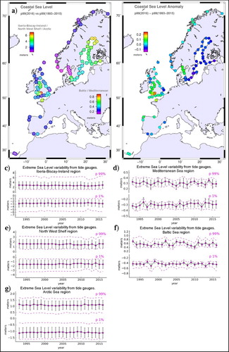
Figure 3.1.2 . (a) 99th percentile surge (external circle: year 2016, inner diamond: 1993–2015 mean value); (b) map of surge anomalies (99th percentile of 2016 – mean of 99th percentile over 1993–2015). Bottom: time series evolution of the 99th and 1st annual percentile levels of surge level averaged for the studied regions (c) Iberia-Biscay-Ireland, (d) Mediterranean Sea, (e) North West Shelf, (f) Baltic Sea, (g) Arctic Sea); average and standard deviation for each year (black), maximum and minimum values in the whole region for each year (magenta).

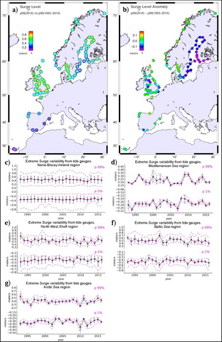
Figure 3.1.3. (a) 99th percentile SST (external circle: year 2016, inner diamond: 2000–2015 mean value); (b) map of SST anomalies (99th percentile of 2016 – mean of 99th percentile over 1993–2015). Bottom: time series evolution of the 99th and 1st annual percentile levels of SST averaged for the studied regions (c) Iberia-Biscay-Ireland, (d) Mediterranean Sea, (e) North West Shelf): average and standard deviation for each year (black), maximum and minimum values in the whole region for each year (magenta).

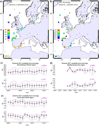
Figure 3.1.4. (a) 99th percentile of SWH (external circle: year 2016, inner diamond: 2000–2015 mean value at each station); (b) map of SWH anomalies (99th percentile of 2016 – mean of 99th percentile over 1993–2015). Bottom: time series evolution of the 99th percentile of SWH averaged for the studied regions (c) Iberia-Biscay-Ireland, (d) Mediterranean Sea, (e) North West Shelf): average and standard deviation for each year (black), maximum and minimum values in the whole region for each year (magenta).

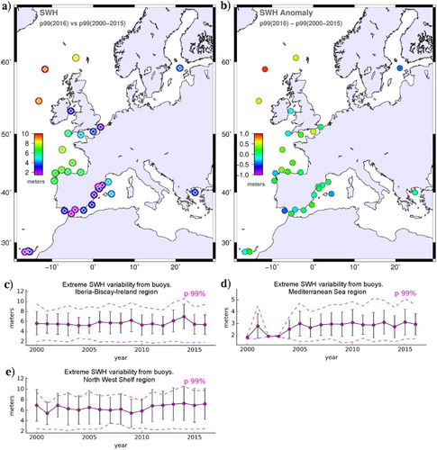
Figure 3.1.5. 99th percentile of SWH (m): (a) mean of annual values over the period 2006–2015; (b) values for year 2016; (c) differences between values in 2016 and the mean of annual values over the period 2006–2015. Circles in the west Mediterranean Sea and north Aegean Sea correspond to equivalent values at buoy locations. The colour inside the circles refers to the corresponding value in the colorbar.

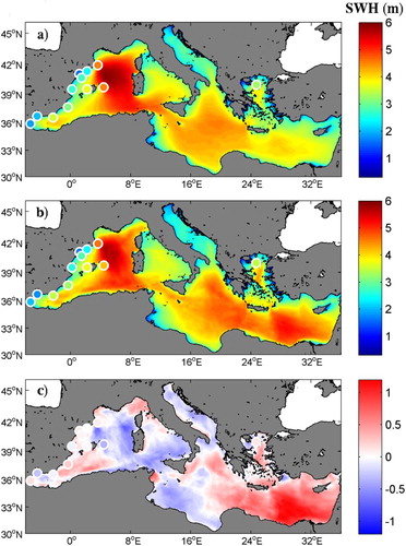
Figure 3.2.1. The Nordic Seas with schematic water pathways showing its overturning circulation from northward flowing Atlantic Water in the surface (red) to southward flowing transformed waters at depth (black). The two branches of the Norwegian Atlantic Current, the Norwegian Atlantic slope current (NwASC) and Norwegian Atlantic front current (NwAFC) are represented by red arrows. The fresh Norwegian Coastal Current (NCC) is indicated in green, while the near-surface East Greenland Current in marked in blue. See Furevik and Nilsen (2005) and Raj et al. 2016 for details. Grey isobaths are drawn for every 600 m. The dashed lines provide the locations of the sections; Faroe-Shetland Channel (FSC), Barents Sea Opening (BSO), Fram Strait (FS) and Denmark Strait (DS).

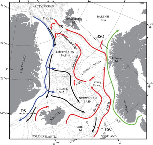
Figure 3.2.2. Volume transport time series of the Atlantic Water flow towards the Arctic. (a) Net volume transport through the Fram Strait (T > 2°C). Positive values towards the north. Black line shows monthly averages and gray-shaded area denotes associated standard deviation. (b) Similar to (a), but showing for the Barents Sea Opening (N70°15′–N74°15′; T > 3°C). Positive values towards the east (into the Barents Sea). (c) Similar to (a), but showing for the Færøy-Shetland Channel (T > 5°C). Positive values towards the north. The model data are based on the product reference 3.2.1 (Sakov et al. 2012) for the years prior to 2016 and the product reference 3.2.2 for 2016. An evaluation of the product reference 3.2.1 is provided in a separate quality information document provided through the Copernicus website (www.marine.copernicus.eu) and in in Lien et al. (2016). Evaluation of the product reference 3.2.2 is found on the Copernicus website, and it is evaluated internally against observations on a weekly basis.

Figure 3.2.3. Volume transport time series of overflow waters as estimated from product reference 3.2.1 (Sakov et al. 2012). The product reference 3.2.2 is used for 2016. (a) Net volume transport of water masses with densities σ _θ > 27.8 through the Denmark Strait. Negative values indicate transport towards the south. Black line shows monthly averages and gray-shaded area denotes associated standard deviation. (b) Similar to (a), but showing for the Færøy-Shetland Channel. (c) Similar to (a), but showing net transport of water masses with σ _θ < 27.8 through the Denmark Strait. An evaluation of the product reference 3.2.1 can be found in the quality information document provided through the Copernicus website (www.marine.copernicus.eu) and in in Lien et al. (2016). Evaluation of the product reference 3.2.2 is found on the Copernicus website, and it is evaluated internally against observations on a weekly basis.

Figure 3.3.1. Mean practical salinity (2002–2014) at 1000 m from the CMEMS product reference 3.3.1. The analysis of the MOW variability is done over the marked boxes: Reservoir, N1, N2, N3, N4 and S1.

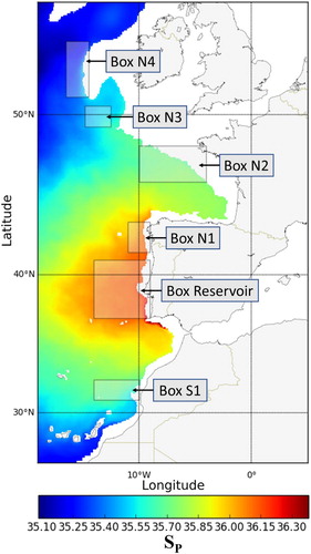
Figure 3.3.2. Seasonal practical salinity (shaded) and currents (arrows) shown only in the area where the zonal salinity maxima takes place. Values under the 85th percentile threshold of salinity computed zonally were masked. For clarity reasons vectors were masked applying a weaker threshold (80th percentile). Winter (DJF)(a), spring (MAM)(b), summer (JJA)(c), and autumn (SON)(d). Averages computed from CMEMS product reference 3.3.1 in the period 2002–2014.

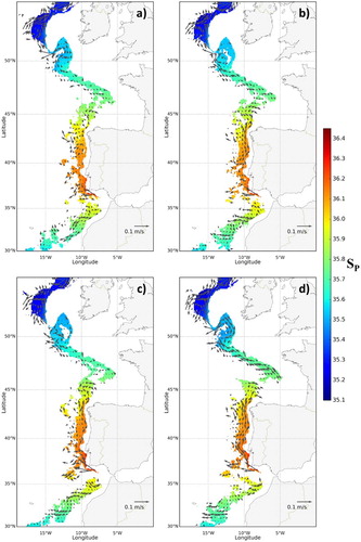
Figure 3.3.3. Practical salinity anomalies averaged in monitoring boxes: Reservoir (a), S1 (b), N1 (c), N2 (d), N3 (e), and N4 (f). Panels show merged results of diverse CMEMS systems: CMEMS product reference 3.3.1 (blue), CMEMS product reference 3.3.2 (orange), and the dispersion of CMEMS gridded products reference 3.3.3–3.3.5 (shaded grey). The trend line of product reference 3.3.1 (dashed black) and trend 99% confidence interval are included.

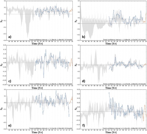
Figure 3.4.1. February monthly climatology of mixed layer depth computed from (product reference 3.4.1, Simoncelli at al. 2014) considering the density criteria Δσ = 0.01 kg/m³ and 10 m reference depth level. Black boxes enclose the areas where deep water formation is known to occur: (1) the Gulf of Lions for the Western Mediterranean Deep Waters (WMDW); (2) the Southern Adriatic Sea Pit for the Eastern Mediterranean Deep Waters (EMDW); (3) the Cretan Sea for the Cretan Intermediate Waters (CIW) and the Cretan Deep Waters (CDW); (4) the Rhodes Gyre for the Levantine Intermediate Waters (LIW) and the Levantine Deep Waters (LDW). The black line in the Sicily Channel (SC) represents the vertical section where annual temperature and salinity time series have been computed and displayed in Figure 3.4.3.

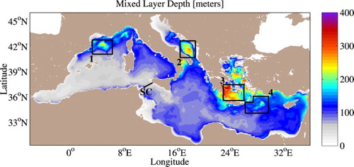
Figure 3.4.2. Water mass formation rates computed in 4 regions (black boxes in Figure 3.4.1) considering different mixed layer density thresholds (see details in Table 3.4.1): (a) in the Gulf of Lion for the Western Mediterranean Deep Waters (WMDW); (b) in the Southern Adriatic region for the Eastern Mediterranean Deep Waters (EMDW); (c) in the Cretan Sea for the Cretan Intermediate Waters (CIW) and the Cretan Deep Waters (CDW); d) in the Rhode Gyre area for the Levantine Intermediate Waters (LIW) and the Levantine Deep Waters (LDW).

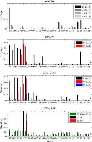
Figure 3.4.3. Annual mean temperature (top) and practical salinity (bottom) of Intermediate Water settling between 200 m depth and the bottom (black line) and on the bottom at 380 m (red line) along the Sicily Channel section (SC) in Figure 3.4.1.

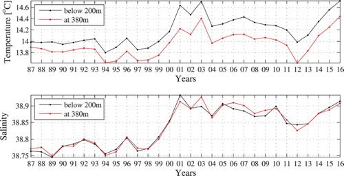
Figure 3.5.1. Location map (Mooring location in Espartel Sill).

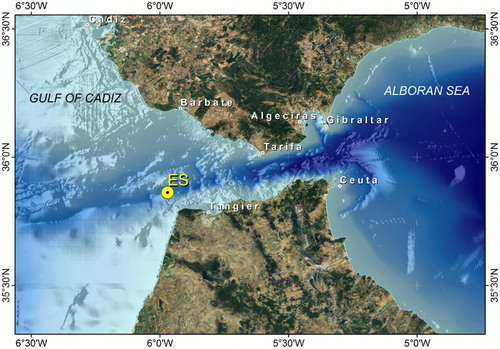
Figure 3.5.2. Subtidal series of (a) potential temperature and (b) salinity series (black dots) measured at Espartel Sill at 348m depth (15m above the sea floor) from September 2004 to September 2016 (product reference 3.5.1) and (red line) the simulated potential temperature and salinity from Mediterranean Sea physical reanalysis (product reference 3.5.2, Simoncelli et al. 2014). For details on the data decimation refers to Naranjo et al. (2017)

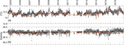
Figure 3.6.1. Typical summer profiles of (a) temperature, (b) practical salinity, (c) Brunt-Väisälä frequency, (d) potential density anomaly and (e) oxygen concentration illustrating the vertical structure of the central Black Sea. Red marks illustrate the diagnostics used to characterise the oxygen content and the Cold Intermediate Layer from in situ profiles (product reference 3.6.1).

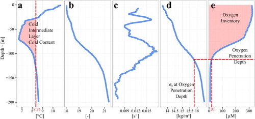
Figure 3.6.2. Interannual variations of oxygen penetration depth on a (a,d) depth and (b,e) density scale and (c,f) oxygen inventory. (a,b,c) Multidecadal trends merging analysis of (black dots) ship-based casts and (blue) Argo floats. For Argo, oxygen penetration depths are also shown using a lower threshold (10 µM) to acknowledge a potential bias between Winkler and Argo oxygen records. The linear trends assessed from the ship-based data set are −0.79 m/yr, −0.0074 kg/m³/yr and −0.144 mol O₂/m²/ yr for (a), (b) and (c), respectively. (d,e,f) Focus on the Argo era (2010–present) and 2016. Note the range of spatial variability visible between the different Argo floats that drift across the Black Sea.

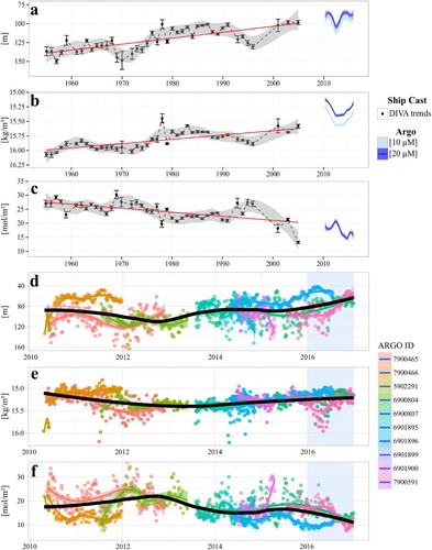
Figure 3.6.3. Estimates of the probability density function for (a) oxygen inventory and (c) cold content within the Cold Intermediate Layer, which is a proxy for convective dense water formation. Panel (b) highlights the ventilating role of cold water formation by depicting the relationship between cold water and oxygen content. Black dots locate the 2016 Argo profiles on this diagram.

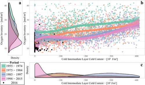
Figure 3.7.1. (a) Map of the Southern Baltic Sea showing locations of the basins. 60 m isodepth is marked with grey line. Blue and red contours show isohalines of the bottom salinities from the regional NRT CMEMS product (3.7.1) for the 1st January (t1) and for the 16th May (t2) of the year 2017. (b) Time series of the maximum distance of the water with salinity greater than 11 g/kg. The distance is shown along the black dashed line starting from point T on subplot (a). Dates t1 and t2 with arrows correspond to dates t1 and t2 on subplots (a) and (c). (c) Time series of basin wide daily mean sea level of the Baltic Sea area derived from the satellite data product (3.7.3) and bottom salinity in the Arkona and Bornholm Basins from the regional NRT CMEMS product reference 3.7.1, smoothed using a 12 day running mean. The grey shaded areas correspond to the winter periods when rapid sea level changes and subsequent inflows occurred. Dates t1 and t2 with arrows correspond to dates t1 and t2 on subplots (a) and (b).

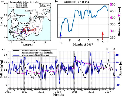
Figure 3.7.2. Hovmöller diagram (time-depth) of salinity in (a) the Arkona Basin and (b) Bornholm Basin from in situ measurements product reference 3.7.2. Black circles show the locations of the deepest measurements at specific date. Red line shows the depth of the mixed layer (smoothed using a 14 day running mean) calculated using modelled density from the product reference 3.7.2 at the respective locations.

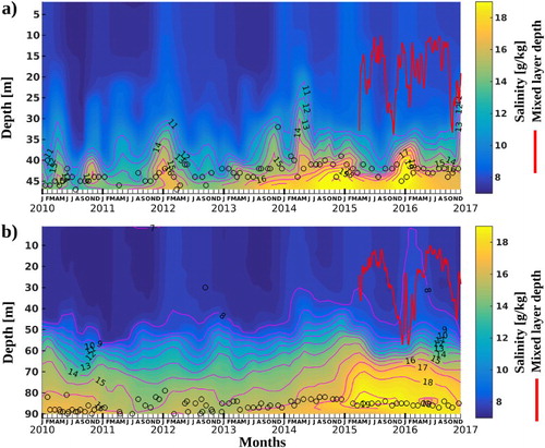
Figure 3.7.3. Hovmöller diagram (time-depth) of (a) salinity, (b) temperature and (c) dissolved oxygen concentration in the Gotland Basin from the in situ measurements product reference 3.7.2. Black circles show the locations of the deepest measurements at specific date. Time series of the mixed layer depth (smoothed using a 14 day running mean) at the Gotland Basin calculated from modelled density in the product reference 3.7.2 are superposed with red line.

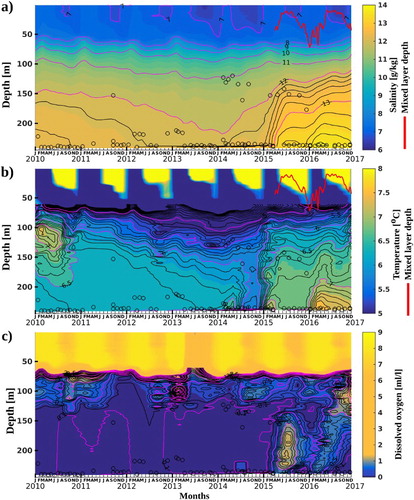
Figure 3.8.1. Subdivisions of the Baltic Sea.

Figure 3.8.2. Baltic Sea summer (10 June to 27 September) chlorophyll-a anomaly field in 2016 (product reference 3.8.1) relative to the 1998–2014 mean field (product reference 3.8.1).

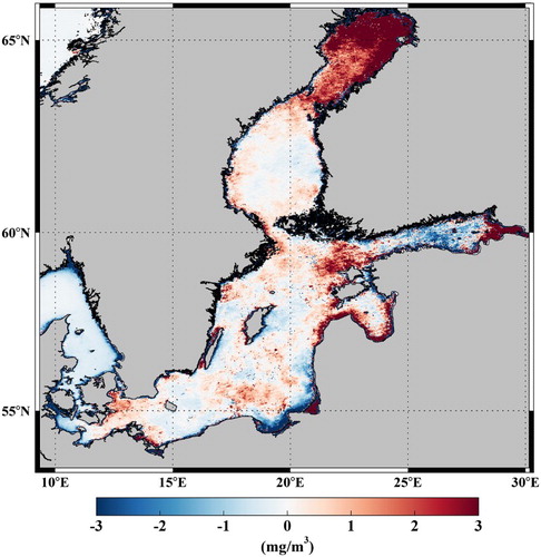
Figure 3.8.3. Time series of summer bloom spatiotemporal coverage (day·km²) (1998–2016) using method by Hansson and Håkansson (2007) and Hansson et al. (2010). Red: surface bloom; blue: subsurface bloom. Results are based on CMEMS product reference 3.8.2.

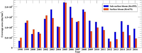
Figure 3.8.4. Baltic Sea potentially hypoxic water volume (O₂ concentration 0–4 mg/L) in the period of 2014–2016 based on the CMEMS product reference 3.8.3.

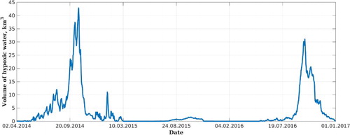
The annual percentiles of slev are referred to local mean sea level at each tide gauge (subtracting the annual 50th percentile). Therefore, as we use relative magnitudes, longer term trends and spatial changes in mean sea level due to ocean circulation, vertical crustal motion and geoid variations are not considered. The 99th and 1st percentiles reflect in this case only the most relevant agents of extreme sea level variability (tide, meteorological effects and monthly and seasonal variations). The main reason for this approach is the lack of a common reference for coastal sea level data at all the stations, but also to avoid undocumented problems of datum in the time series. The surge data were obtained after removal of the tide and the mean seasonal cycle (annual tidal constants averaged for the whole period).

The 99th percentile of slev (Figure 3.1.1(a), notice the two colour bars) reflects the large spatial variation of the tidal amplitude along the European coasts, ranging from near 7 m over local mean sea level in the Bristol Channel to less than 0.2 m in the Western Mediterranean, while Figure 3.1.2 shows that the surge ranges from approximately −0.8 to 1.0 m, extreme values considering all the stations, although the regions mostly show less variability. This reflects the potential influence of this component of sea level not only in high extremes but also in lowering coastal sea levels (if a negative value coincides with a low tide).

There is a reasonable spatial coherence of the 2016 anomaly for slev and surge (Figures 3.1.1(b) and 3.1.2(b)). The most interesting result is the negative anomalies of 2016 highest sea levels at all the stations in the Baltic Sea. The largest negative values are found along the southeastern coast of Sweden (up to 10 cm lower than 1993–2015 mean). A slight decrease is also evident in the evolution of the lowest sea levels (1st percentile) averaged for this basin (Figure 3.1.1(f)): 2016 shows the second largest minimum value in the period 1993–2016 (the first one appears in 1998). Section 4.5 presents a more detailed discussion of this extreme in low sea level in the Northern Baltic Sea and points to the influence of the ice melting and prevailing northeasterly winds storms in lowering sea levels in this area (minimum sea levels in 2016 were recorded at Kemi tide gauge, Gulf of Bothnia, see Figure 4.5.1 in Section 4.5). Negative anomalies in the Baltic are even more clear in the 99th percentile for surge (Figure 3.1.2(b)), notice the largest negative anomalies in the Gulf of Finland), indicating the great influence of the meteorological component on the total sea level variability in this basin with small tides (something similar applies to the Mediterranean Sea). This could also be related to the reduction of storminess in the Baltic in 2016 (Kristine S. Madsen, DMI, personal communication: no storm surges in 2016 from Danish tide gauges in the Baltic). This negative anomaly in the 99th percentile of sea level and surge in the Baltic could be related to the negative trends found by Marcos and Woodworth (2017) for the last decades at several tide gauges in the basin, and contrasts, interestingly, with the positive anomaly obtained for absolute mean sea level from altimetry data (see Section 1.5, chapter 1). Notice that the tide gauge data used here are not expected to be contaminated by the postglacial rebound of Scandinavia because annual means have been substracted from the data; therefore, the negative anomalies obtained here for the extreme sea levels variability should not be related to the land uplift in this basin.

Slightly positive anomalies of maximum slev are observed, however, for most of the stations of the Iberia-Biscay-Ireland, North West Shelf and Arctic Sea regions, except at the Gulf of Cadiz, western Scotland and southeast England, which present small negative anomalies. This contrasts in the Iberia-Biscay-Ireland region to the anomalies in the surge level (Figure 3.1.2(b)) that are close to zero or negative everywhere.

The largest positive anomalies of slev in 2016 are present at a couple of stations in the Bristol Channel, exceeding the historical mean up to 20 cm in Avonmouth (Figure 3.1.1(b)). The increase in 2016 of maximum coastal sea levels in this estuary is apparently not related to the surge, according to Figure 3.1.2(b). However, as non-linear shallow water effects complicate the computation of the tidal signal here (Hibbert et al. 2015), the results for the surge at this estuary should be considered carefully and further analysed in the future.

In the North West Shelf, maximum sea levels (99th percentile) in 2016 are similar to the mean and 2015 values for the whole region. Regarding the surge component, the 99th percentile regional average is lower than in 2015, lower than the historical mean on the southeastern coast of England, and larger than the historical mean along the Swedish coast.

This study uses hourly sea level data available in the different In Situ Thematic Assembly Centre (INSTAC) Dissemination Units at the time of writing, therefore higher frequency oscillations caused by meteotsunamis, infragravity waves, etc, that could affect the final total extreme sea level at the tide gauge in some cases, are not considered.

3.1.2. Extreme SSTs from CMEMS moorings

Based on our analysis of the data available in the different INSTAC regions (product reference 3.1.1–3.1.8), the analysis of SST from moorings is focused this year on the period 2000–2016 as a starting point for future reports. Results are displayed in Figure 3.1.3: the stations considered for the North West Shelf area are the ones located in the northwest of the British Isles and the two located in the eastern part of the English Channel. The rest of stations in the Atlantic belong to the Iberia-Biscay-Ireland region.

Despite the short length of the time series (<16 years), several interesting features are observed: for example, Figure 3.1.3(a) shows a reasonable spatial coherence in the maximum values and an expected decrease of SST northwards, with the highest values recorded in the Mediterranean Sea and the lowest in the open ocean stations of the North Atlantic (54°N–60°N); moreover, the temperatures in the Baltic are higher for the same latitudes.

This spatial coherence is less evident in the anomalies of 2016 99th percentile (Figure 3.1.3(b)), where local effects may become more evident. The largest positive anomaly (>1°C) is observed in the Gulf of Cadiz (Figure 3.1.3(b)); 2016 has been a hot year in this area with maximum temperatures exceeding 24°C during the three summer months. However, in the western Atlantic stations (North of British Islands and Canary Islands) the 99th percentile in 2016 is lower than the historical mean, in coherence with the cold anomaly detected in the North Atlantic (see Section 4.3). In the Canary Islands, during the summer of 2016 the highest temperatures remained around 24°C, below the highest values of the averaged year (usually over 24.5°C).

In the Iberia-Biscay-Ireland area, the unusual low temperatures recorded in Europe during 2004 and 2005 are reflected in the 1st percentile temporal evolution for this region (Figure 3.1.3(c)). In the Mediterranean Sea, Figure 3.1.3(d) shows that, in the areas with measurements (West Med and Aegean Sea), 2016 has been a smooth weather year, with milder temperatures in winter and summer than previous years (results before year 2007 have been masked in this figure because only one or two stations were in operation those years). An increase of the minimum or 1st percentile values is also clear in 2016 in the Mediterranean. In the North West Shelf area, the 1st percentile shows a noticeable increase in 2007 and 2014. The winters these two years were milder than usual (temperatures going down to around 10°C when usually they reach 7–8°C). The figure also shows that 2006 displayed the largest temperature range (highest 99th percentile and lowest 1st percentile) with SST in the English Channel close to 6°C in winter and over 18°C in summer.

3.1.3. Extreme SWHs from CMEMS moorings

As of SST, the period 2000–2016 was used for SWH (same buoys), with the same distribution of stations for each region. Results are displayed in Figure 3.1.4. In this case, 1st percentiles are not displayed in the time series (Figures 3.1.4(c–e)) because minimum wave heights are not of interest.

As a general view in the European coasts (Figure 3.1.4(a)), the maximum wave heights are observed in the two stations in the northwest of Great Britain (99th percentile close to 10 m). Extreme wave heights are lower in the Canary Islands, South of Spain, English Channel, Irish Sea, Mediterranean and Baltic Seas. The location of the buoys (coastal or in the open ocean) can affect these extreme values being higher for deep water buoys and lower for those ones closed to the coast and affected by the local bathymetry that attenuates and dissipates the wave energy.

The wave data coverage from buoys in the European seas is insufficient for long-term studies, which could explain why the available data do not reveal a significant trend in SWH for the last years. 2016 was an average year in most of the studied regions, except the positive anomalies (up to 1 m, Figure 3.1.4(b)) observed in the two stations in the northwest of Great Britain, due to two severe storms that passed over this area. Negative 2016 anomaly of highest SWH is observed in the only buoy available in the Baltic Sea. This is coherent with a reduction of the storminess in 2016 in this area, and with the negative anomalies observed in the storm surge component of sea level (see Section 3.1.1).

Regarding the temporal evolution of extremes, the highest waves in the Iberia-Biscay-Ireland and North West Shelf regions correspond to 2014 (Figure 3.1.4(c,e)), when the number of extreme storms in the area was higher than usual (4–5 extreme events with SWH over 10 m, while during an average year only 1–2 events are recorded). 2015 and 2016 were typical average years in the Iberia-Biscay-Ireland area. It could seem that these two regions are influenced by the same storms originated in the North Atlantic, but the results in the percentiles study differ. The Atlantic storms trajectory variations between north and south respect to the British Isles can lead to appreciable differences in the wave measurements in both regions. The second 99th percentile maximum observed in 2009 for Iberia-Biscay-Ireland is not present in the North West Shelf. This year, the cyclogenesis Klaus passed over the Bay of Biscay (affecting only the Iberia-Biscay-Ireland area) and several buoys recorded their maximum ever. This second 99th percentile maximum appears in 2013 in the North West Shelf, due to an extreme storm in the north of the British Isles that produced the highest-ever SWH recorded by a buoy (WMO 2016), reaching 19 m.

In the Mediterranean Sea, the extreme SWH variability (Figure 3.1.4(d)) is not meaningful before 2004 due to a lack of measuring stations. In the graph, some relative maximums are showed in years 2005, 2010 and 2015 corresponding to the occurrence of severe storms in the area.

3.1.4 Extreme SWHs from MED-MFC model reanalysis

In the case of SWH in the Mediterranean Sea, we had access to the Mediterranean Monitoring and Forecasting Center (Med-MFC) multi-year wave hindcast covering the period 2006–2016 (product reference 3.1.9). The 99th percentile of SWH has been computed for every grid point (1/24° resolution) and displayed in Figure 3.1.5. Results from the wave buoys in the region are superimposed on the map. For this, the analysis of buoy SWH data was repeated under the same conditions as for model data, i.e. focusing on the period 2006–2016 (at least 7 years of data with completeness index over 70% in this period for a station to be considered).

The mean annual 99th percentile of SWH for the period 2006–2015 (Figure 3.1.5(a)) varies from 0.357 m to 5.923 m. The lowest values are mainly found along the northeastern Mediterranean coast (Adriatic, Aegean and Levantine coast) and in the Gulf of Gabes. The highest values are located where high winds and long fetch are simultaneously present. Specifically, such values extend from the Gulf of Lion to the southwestern Sardinia through the Balearic Sea. They result from northerly winds (Mistral or Tramontana) – dominant in the western Mediterranean Sea – accelerated by orography (Menéndez et al. 2014) and acting over a large area. High values (>5 m) are sustained southwards approaching the Algerian coast and extending to the Strait of Sicily. Values are generally above 4 m for a considerable part of the southern Mediterranean Sea. In the Ionian Sea, the northerly Mistral wind is still the main cause of high waves whilst in the Aegean and Levantine Seas, high waves are caused by the northerly Bora winds, prevalent in winter, and the northerly Etesian winds, prevalent in summer (Lionello et al. 2006; Chronis et al. 2011; Menéndez et al. 2014).

Values obtained from the buoys are in close agreement with model results with the former being somewhat lower at most locations (Figure 3.1.5). Only offshore from Barcelona and west of Mallorca are buoy results higher with respect to both the 2006–2015 mean and 2016 values. The greatest discrepancies between model and buoy results happen at the buoy located east of the Balearic Islands and reach 0.5 m.

In 2016, there is an obvious increase in the values of the 99th percentile of SWH relative to the 2006–2015 mean over the eastern Mediterranean Sea, east of about 18°E, especially over the Levantine Sea (up to 1.2 m increase) (Figure 3.1.5(c)). To the west of 18°E, increased values are observed along most of the east facing north Mediterranean coastline, in the Gulf of Gabes and the south Balearic Sea. Otherwise, reduced or unchanged values are observed. In general, in the western Mediterranean Sea the differences between the means for 2016 and the 2006–2015 period are mostly in the range of ±0.5 m in accordance with similar results from buoy measurements presented in Figure 3.1.4.

3.2. North Atlantic – Arctic exchanges

Leading author: Vidar Lien.

Contributing author: Roshin P. Raj.

Statement of main outcome: A strong increase in the volume and heat of Atlantic Water transported to the Arctic Ocean towards the end of 2016. However, upstream in the Færøy-Shetland Channel, the results indicate a decrease in the northward transport of Atlantic Water in 2016, linked to a temperature decrease in the North Atlantic. This change is likely to affect the Nordic Seas and eventually the Arctic Ocean heat budget in coming years, due to the highly advective nature of the Nordic Seas.

Products used:

Table

Ref. No.	Product name & type	Documentation
3.2.1	ARCTIC_REANALYSIS_PHYS_002_003Reanalysis	QUID: http://marine.copernicus.eu/documents/QUID/CMEMS-ARC-QUID-002-001a.pdf PUM: http://marine.copernicus.eu/documents/PUM/CMEMS-ARC-PUM-002-ALL.pdf
3.2.2	ARCTIC_ANALYSIS_FORECAST_PHYS_002_001_a Model	QUID: http://marine.copernicus.eu/documents/QUID/CMEMS-ARC-QUID-002-003.pdf PUM: http://marine.copernicus.eu/documents/PUM/CMEMS-ARC-PUM-002-ALL.pdf

The northward flow of relatively warm and saline Atlantic Water through the eastern Nordic Seas and into the Arctic, balanced by outflow of cold Arctic water masses through the western Nordic Seas, governs the exchanges between the North Atlantic and the Arctic as well as the distribution of oceanic heat within the Arctic (e.g. Mauritzen et al. 2011; Rudels 2012; Figure 3.2.1). Thus, the warm and saline Atlantic Water transported from the North Atlantic to the Arctic through the Nordic Seas via the Norwegian Atlantic Current plays a major role in the global climate system (Rhines et al. 2008). The heat transport associated with the inflow of Atlantic Water to the Nordic Seas (relative to 0°C) is estimated to be on the order of 250 TW (Hansen et al. 2003, Segtnan et al. 2011). About half of this heat is lost due to air-sea interaction or lateral eddy mixing before the Atlantic Water leaves the Nordic Seas through the Barents Sea opening or through the Fram Strait (Segtnan et al. 2011). The fate of the remaining ocean heat transported towards the Arctic depends on the downstream pathway: the Atlantic Water entering the Arctic through the Fram Strait retains a large part of its heat as it flows cyclonically along the Arctic Ocean shelf slope (e.g. Polyakov et al. 2005, 2017), whereas the Atlantic Water that enters the Barents Sea loses most of its heat before it enters the Arctic Ocean through the St. Anna Trough (e.g. Lien and Trofimov 2013).

The Atlantic Water transported poleward has been found to significant influence the sea-ice cover in the Barents Sea (Sandø et al. 2010; Årthun et al. 2012; Onarheim et al. 2015) and near Svalbard (Piechura and Walczowski 2009). Furthermore, the Atlantic Water flow through the eastern Nordic seas and its associated heat loss and densification are important factors for the formation of overflow waters in the region (Mauritzen 1996; Eldevik et al. 2009). These overflow waters together with those generated in the Arctic, exit over the Greenland Scotland Ridge, which further contributes to the North Atlantic Deep Water (Dickson and Brown 1994) and thus play an important role in the Atlantic Meridional Overturning Circulation (Eldevik et al. 2009; Ch. 2.6). In addition to the transport of heat, the Atlantic Water also transports nutrients and zooplankton (e.g. Sundby 2000), and it carries large amounts of ichthyoplankton of commercially important species, such as Arcto-Norwegian cod (Gadus morhua) and Norwegian spring-spawning herring (Clupea harengus) along the Norwegian coast. The Atlantic Water flow thus plays an integral part in defining both the physical and biological border between the boreal and Arctic realm. Variability of the Atlantic Water flow to the Barents Sea has been found to move the position of the ice edge (Onarheim et al. 2015) as well as the habitats of the various species in the Barents Sea ecosystem (Fossheim et al. 2015).

The Atlantic Water flow towards the Arctic has been monitored regularly by direct current measurements for a couple of decades in key sections (see Figure 3.2.1): the Færøy-Shetland Channel (since 1994; Berx et al. 2013); the Faroe North section (Hansen et al. 2015); the Svinøy Northwest section (since 1995; Orvik et al. 2001; Mork and Skagseth 2010); The Barents Sea Opening (since 1997; Ingvaldsen et al. 2002); and the Fram Strait (since 1997; Schauer et al. 2004). In addition, these sections are monitored through hydrographic sections with the coverage frequencies varying from one to several per year. Here, we present estimates of ocean volume transports representing North Atlantic – Arctic exchanges based on TOPAZ reanalysis (during 1993–2015; Xie et al. 2016; product reference 3.2.1, see below) and real-time TOPAZ forecast data (during 2016; product reference 3.2.2, see below) and compare them with the observation-based estimates (from 1993 onwards). Note that in the rest of the section, we use the term ‘model-based’ for the combined TOPAZ reanalysis (during 1993–2015) and TOPAZ real-time data (during 2016).

The flow of Atlantic Water through the Færøy-Shetland Channel amounts to 2.7 Sv (Berx et al. 2013). The corresponding model-based estimate was 1.9 Sv for the period 1993–2016. Notably, the volume transport during the years 2014 to 2016 is significantly lower than the long-term mean (1993–2016; Figure 3.2.2(a). All months, except September, had lower than average Atlantic Water inflow in 2016, in comparison to the long-term (1993–2016) model mean. These volume transport anomalies are also associated with negative heat transport anomalies entering the Nordic Seas (not shown). The strong reduction seen in the modelled Atlantic Water inflow in recent years is most likely related to the negative temperature anomalies in the upstream North Atlantic in the years 2014–2016 (see Figure 2.5.1 and 2.5.2, Section 2.9; Section 4.3), with the consequences expected to spread downstream into the Nordic Seas in the coming years, due to the highly advective nature of the Nordic Seas (e.g. Furevik 2001). Although the temperature anomalies do not necessarily imply lower Atlantic Water volume transport northwards, the estimated amount of Atlantic Water is likely to be reduced due to the temperature criterion (T > 5°C) used when calculating the volume transport.

Downstream in the Barents Sea Opening, the model indicates a long-term average net Atlantic Water inflow of 2.2 Sv (Figure 3.2.2(b)), as compared with the long-term estimate from observations of 1.8 Sv (Smedsrud et al. 2013). During 2016, the modelled Atlantic Water inflow to the Barents Sea was below average throughout the whole year. The transport anomaly is more than two standard deviations below the seasonal long-term average in April and June, i.e. spring and early summer, when the concentration of zooplankton and ichthyoplankton within the Atlantic Water is high (Sundby et al. 2013).

In the Fram Strait, the model results indicate that the volume transport of Atlantic Water in 2016 was comparable to the previous years, except for a strong increase towards the end of the year (Figure 3.2.2(c)). However, in comparison to 2005–2010, the northward flow of Atlantic Water was lower in 2016. The averaged (1993–2016) modelled Atlantic Water volume transport northwards through the Fram Strait (0.9 Sv) is less than the observation-based estimates (3.0 Sv; 1997–2010; Beszczynska-Möller et al. 2012). The model data indicate an apparent shift in the flow regime of Atlantic Water in 2005, with a distinct increase as compared with previous years. This temporary increase in Atlantic Water transport may be explained by increased temperature in the West Spitsbergen Current during the period 2005–2010 (e.g. Walczowski et al. 2012), which caused a larger fraction of the water mass to be characterised as Atlantic Water (T > 2°C). This temperature and associated Atlantic Water volume and heat transport increase, has many impacts on the Eurasian Arctic, ranging from hydrography (e.g. Polyakov et al. 2012) to sea-ice conditions (e.g. Polyakov et al. 2017) and distribution of species (e.g. Fossheim et al. 2015), as well as the net carbon uptake at high latitudes (e.g. Smedsrud et al. 2013).

The northward flow of Atlantic Water is partly compensated by southward flow of colder and denser overflow water from the Nordic Seas to the northern North Atlantic, in addition to colder and less saline surface waters carried by the East Greenland Current (see Figure 3.2.1). The overflow of dense water consists of several branches; one through the Faroe-Shetland Channel (e.g. Borenäs and Lundberg 2004), one over the Iceland Faroe Ridge (Hansen and Østerhus 2000), and one through the Denmark Strait (e.g. Jochumsen et al. 2017), with the latter being the largest accounting for about 50% of the total overflow (Jochumsen et al. 2017). The dense water overflow (defined by σ_θ  > 27.8) through these openings represents the integrated contribution from the dense water formation within the Arctic to the Arctic-North Atlantic exchanges. Such dense water formation mainly occurs in hotspots including the banks within the Barents Sea (Midttun 1985), Storfjorden in the Svalbard archipelago (e.g. Skogseth et al. 2008) and the area surrounding the archipelagos Franz Josef Land and Severnaya Zemlya (e.g. Martin and Cavalieri 1989), although some formation also takes place in the open ocean including the Greenland and Norwegian seas (e.g. Clarke et al. 1990). However, common to all the formation sites is the availability of Atlantic-derived water masses, which yields high enough salinities (typically S > 34.9) for the water masses to become dense enough to sink into the deep ocean through cooling and/or brine rejection associated with ice freezing.

Model-based estimates of the Denmark Strait overflow, as defined by water masses with σ _θ> 27.8, yields an average of 1.1 Sv during the period 1996–2011, one third of the volume transport estimated based on direct current observations for the same period (3.2 Sv, Jochumsen et al. 2017; Figure 3.2.3(a). The model estimates for 2016 (0.6 Sv) is also less than the long-term average. The model results are contrary to the observations, both with respect to the lack of a long-term trend in the observations and the magnitude of the interannual variability, found to be 0.4 Sv in the observations (i.e. ∼10% of the long-term average; Jochumsen et al. 2017). At the Færøy-Shetland Channel, the model results show a decrease in the dense water (σ_θ < 27.8) outflow during the recent years (Figure 3.2.3, (b). In 2016, the overflow estimate was less than half (0.2 Sv) of the 1993–2016 modelled average of 0.5 Sv, which, in turn, is significantly lower than the observation-based estimates (2.2 Sv; Hansen et al. 2016). While the model estimates fall short of the observation-based estimates of overflow water entering the North Atlantic, the model results agree with a general pattern of a weakening of the Atlantic Meridional Overturning Circulation, and hence, the overflow circulation in the recent decade (see Section 2.6).

In addition to the dense water overflow, the East Greenland Current carries cold and less saline surface waters from the Arctic to the North Atlantic through the Denmark Strait. The model results show a net, southward volume transport of water masses with a density σ_θ < 27.8 of 0.9 Sv, on average during the period 1993–2016 (Figure 3.2.3(c). The volume transport in 2016 is comparable to recent years and to the long-term average. Few observation-based estimates of the volume transport carried by the East Greenland Current exist, and especially so for extended time periods. A densely-sampling mooring array deployed in 2011–2012 indicates a net southward volume transport of ∼2 Sv, when calculating for water masses with a density σ_θ  < 27.8 (de Steur et al. 2017).

3.3. Characterisation of Mediterranean outflow water in the Iberia-Gulf of Biscay-Ireland region

Leading authors: Álvaro Pascual, Bruno Levier, Marcos Sotillo.

Contributing authors: Nathalie Verbrugge, Roland Aznar, Bernard Le Cann.

Statement of the outcome: In 2015–2016, the salinity anomalies in the different monitoring boxes are included in the ranges of variability established by the respective time series in the period 2003–2015. Thus, the salinity values in the period 2015–2016 are similar to the average values seen in the previous years 1993–2015. With the exception of the monitoring box N3, the maintenance of salinity anomalies in 2016 supposes a continuous normal behaviour in all monitoring boxes. On the contrary, in box N3 the salinity in 2014 shows a strong negative anomaly, therefore the results obtained in 2015–2016 presumes the finalisation of such negative event. The study describes the presence of a salinity trend in box N4 affecting the period 2003–2015, however, the period 2012–2016 might show an inversion of the trend (change of phase to a positive trend), but this reverse will have to be confirmed when the time series is extended.

Products used:

Table

Ref. No.	Product name & type	Documentation
3.3.1	IBI_REANALYSIS_PHYS_005_002 Reanalysis	QUID: http://marine.copernicus.eu/documents/QUID/CMEMS-IBI-QUID-005-002.pdf PUM: http://marine.copernicus.eu/documents/PUM/CMEMS-IBI-PUM-005-002.pdf
3.3.2	IBI_ANALYSIS_FORECAST_PHYS_005_001_b Model	QUID: http://marine.copernicus.eu/documents/QUID/CMEMS-IBI-QUID-005-001.pdf PUM: http://marine.copernicus.eu/documents/PUM/CMEMS-IBI-PUM-005-001.pdf
3.3.3	GLOBAL_REANALYSIS_PHY_001_025	QUID: http://marine.copernicus.eu/documents/QUID/CMEMS-GLO-QUID-001-025-011-017.pdf PUM: http://marine.copernicus.eu/documents/PUM/CMEMS-GLO-PUM-001-025-011-017.pdf
3.3.4	GLOBAL_REP_PHY_001_021	QUID: http://marine.copernicus.eu/documents/QUID/CMEMS-GLO-QUID-001-021.pdf PUM: http://marine.copernicus.eu/documents/PUM/CMEMS-GLO-PUM-001-021.pdf
3.3.5	INSITU_GLO_TS_OA_REP_OBSERVATIONS_013_002_b	QUID: http://marine.copernicus.eu/documents/QUID/CMEMS-INS-QUID-013-002b.pdf PUM: http://marine.copernicus.eu/documents/PUM/CMEMS-INS-PUM-013-002-ab.pdf

The Mediterranean Outflow Water (MOW) is a saline and warm water mass occupying the eastern North Atlantic intermediate depths, it is produced at the Gulf of Cadiz as a result of intense mixing processes between the western Mediterranean deep waters and the North Atlantic Central Water. After the Mediterranean water overpasses the Strait of Gibraltar sill, the denser Mediterranean water cascades along the Gulf of Cadiz slope and progressively entrains the ambient North Atlantic Central Water to form the MOW. This process causes a significant decrease of salinity and temperature of MOW which finally reaches a buoyant depth around 1000 m depth. After surpassing Cape St. Vincent, MOW is accumulated in an area west of the Iberian Peninsula (Figure 3.7.1) and spreads from this reservoir following two main advective pathways (Iorga and Lozier 1999): (i) a westward branch to the central Atlantic where the transport is totally accounted by mesoscale fluxes and westward propagation of eddies (Reid 1979; Mazé et al. 1997), and (ii) a poleward pathway driven by the Iberian Poleward Current, which follows the bathymetry of the Iberian Peninsula, continental slope of Bay of Biscay, and reaches high latitudes as Rockall Trough at 56°N (Holliday et al. 2008; Lozier and Stewart 2008).

The extension of the area affected by MOW and its physical and chemical properties are attached to several oceanographic processes resulting in variability at different time scales, from the seasonal scale up to long-term scales (Garcia Lafuente et al. 2007; Leadbetter et al. 2007; Holliday et al. 2008; Bozec et al. 2011). Moreover, the importance of the heat and salt transport promoted by the MOW flow has implications beyond the boundaries of the Iberia-Bay of Biscay-Ireland (IBI) domain (Reid 1979, Paillet et al. 1998, Van Aken 2000). Therefore, the establishment of long-term monitoring programmes to observe the MOW variability and transports becomes important to have a proper understanding of the climate system and its evolution.

The present study provides a monitoring of seasonal and interannual variability of MOW in the Eastern North Atlantic. Several CMEMS products have been used to obtain reliable monitoring indices of MOW (reference products 3.3.1, 3.3.2, 3.3.3, 3.3.4, and 3.3.5). Our results show that seasonal variability mainly affects continental slopes of Iberian Peninsula and Celtic-Armorican seas. The seasonal variability is not homogeneous in all the areas affected by MOW, the wide spatial coverage of IBI reveals the differences in seasonality of specific areas. A remarkable seasonal regime is found in Porcupine Sea Bight where the circulation pattern is strongly affected by annual cycles presenting different circulation features in fall-winter and spring-summer.

The analysis of 1000 m salinity in monitoring boxes has identified the boxes N1, N3 and N4 as areas with high interannual variability. Such perturbations are inducted by the high dynamic variability found in these areas due to the complex bathymetry that favours variable circulation patterns leading to consequent variations in salinity fields. The trends of monitoring indexes reveal a negative tendency of salinity at 1000 m affecting box N4. This trend is consistent with previous studies (Holliday et al. 2008; Bozec et al. 2011). All these studies cover up to the early 2000s, therefore they only show positive trends of salinity in Rockall Trough. The update of the timeseries of salinity, indicates the trend reversal (∼−0.02 PSU/decade) in the period 2003–2015.

The selected monitoring areas provide a reliable representation of MOW variability (Figure 3.3.1). A bigger reference box identifies the MOW core reservoir (as described in Daniault et al. 1994). Other boxes were selected as representative areas in view of their specific variability of currents and salinity. A climatic study of salinity sections along latitudes (45° N, 40° N, 35.9° N, and 30.6° N) and longitudes (15°W, 10°W, 8°W and 5°W) together with bibliographic support (Prieto et al. 2013) has led us to define 1000 m as the reference MOW core depth. The seasonal variability analysis of maximum zonal salinity maps (Figure 3.3.2) has highlighted the selected regions (N1, N2, N3, and S1) as areas with significant hydrographic seasonality. The literature describes N4 as location where the influence of MOW shows a high interannual variability (Holliday 2003; Holliday et al. 2008; Lozier and Stewart 2008; Bozec et al. 2011).

The distinctive MOW salinity can be used to depict its distribution in the IBI domain. Figure 3.3.2 shows the 1000 m salinity and currents seasonally averaged. Both fields have been masked by removing all data under the 85th percentile of zonally estimated salinity and thus just show data associated to the zonal salinity maxima. Maps indicate the presence of two MOW pathways, the northward branch along the European continental slope up to Rockall Trough, and the south pathway promoted by the injection of Mediterranean Outflow Water produced by the 35°N and 9°W cyclonic gyre (Iorga and Lozier 1999). As water moves away from the reservoir area, the Mediterranean Outflow Water salinity decreases, from P _S= 36.2 in the reservoir area to P _S= 35.2 in Rockall Trough. Currents associated with the northward branch show a strong seasonal cycle, particularly in the Iberian Peninsula margins, the Celtic-Armorican shelf and Porcupine Sea Bight. The seasonal cycle is characterised by an intensification of the narrow jet along the continental shelf in autumn (Figure 3.3.2(b), SON) and its collapse in winter (Figure 3.3.2(a), DJF). The autumn intensification of the flow induces a characteristic seasonal circulation in Porcupine Sea Bight, the intense jet enters the bight following the bathymetry, this circulation pattern is present but weaker during the winter months. During spring (Figure 3.3.2(b), MAM) and summer (Figure 3.3.2(c), JJA), the currents weaken, which establishes a flow crossing the bight entrance without entering it.

The MOW variability is monitored in the defined boxes by computing the salinity anomaly relative to the monthly mean salinity between 1993 and 2014 provided by CMEMS product reference 3.3.1 (Figure 3.3.3). The analysis of the anomalies reveals the existence of a specific variability affecting each monitoring box. It is remarkable the high variability found in boxes N1, N3 and N4 in opposition to the low range of variability characterising boxes Reservoir and N2. The increase of variability is strongly influenced by the existence of local dynamic processes affecting each box: (1) The intensity of currents in Porcupine show a strong relevance on the circulation patterns of the Box N3 (Figure 3.3.2). (2) The circulation pattern in the Box N1 is affected by the presence of the Galician Bank leading to the eventual appearance of a secondary branch of MOW around the promontory (Prieto et al. 2013). (3) Box N4 is strongly affected by several hydrographic processes such as the interaction of MOW with Labrador Sea Water, the presence of the North Atlantic current, and the influence of the subpolar front (Lozier and Stewart 2008).

There are no significant trends in monitoring boxes N1, N2, N3, S1, and Reservoir. The results obtained for Box N4 (Figure 3.3.3(f)) show a significant negative trend (∼−0.02 PSU/decade) affecting the period covered by product reference 3.3.1 (2003–2015). The salinity anomalies obtained with other CMEMS products (shaded grey area) provide a similar result for this period, however, the extended temporal coverage of this product indicates the inversion in 2003–2004 of a previous positive trend affecting the period 1993–2003. This finding is consistent with Bozec et al. (2011) who described a positive trend of salinity in the period 1975–1995. In this work it is also possible to appreciate the initial stages of the inversion of trend in the period 2000–2005. Trends of salinity anomalies in Rockall Trough has been associated in the literature with the (eastward) westward shifts of the subpolar front (Holliday 2003; Holliday et al. 2008) and with salinity anomalies along the westward pathway in the subtropical gyre (Bozec et al. 2011).

3.4. Water mass formation processes in the Mediterranean sea over the past 30 years

Leading authors: Simona Simoncelli and Nadia Pinardi.

Contributing authors: Claudia Fratianni, Clotilde Dubois, Giulio Notarstefano.

Statement of outcome: The Mediterranean Sea reanalysis covering the latest 30 years (1987–2016) is able to reproduce both Eastern Mediterranean Transient and Western Mediterranean Transition phenomena and catches the principal water mass formation events reported in the literature. This will permit constant monitoring of the open ocean deep convection process in the Mediterranean Sea and a better understanding of the multiple drivers of the general overturning circulation at interannual and multidecadal time scales. 2016 does not present significant events of deep water formation in the Mediterranean Sea.

Products used:

Table

Ref. No.	Product name & type	Documentation
3.4.1	MEDSEA_REANALYSIS_PHYS_006_004 Reanalysis	PUM: http://marine.copernicus.eu/documents/PUM/CMEMS-MED-PUM-006-004.pdf QUID: http://marine.copernicus.eu/documents/QUID/CMEMS-MED-QUID-006-004.pdf DOI: https://doi.org/10.25423/medsea_reanalysis_phys_006_004

The formation of intermediate and deep water masses is one of the most important processes occurring in the Mediterranean Sea, being a component of its general overturning circulation. This circulation varies at interannual and multidecadal time scales and it is composed of an upper zonal cell (Zonal Overturning Circulation) and two main meridional cells in the western and eastern Mediterranean (Pinardi and Masetti 2000).

The Zonal Overturning Circulation is driven by the Atlantic Water inflow at Gibraltar, heading for the Eastern Mediterranean through the Sicily Channel, becoming the Atlantic Ionian Stream and moving towards the Levantine Sea, where it transforms into Intermediate Water under the influence of atmospheric forcing and salinity preconditioning. Intermediate Water characterises the layer between 200 and 400 m, sinks in the Northern Levantine region (Levantine Intermediate Water) or the Cretan Sea (Cretan Intermediate Water) and it flows back to the Sicily Channel to enter the Western Mediterranean on its way back to Gibraltar (Pinardi et al. 2015). The Intermediate Water influences the Western Meridional Overturning Circulation triggered by the deep water formation process occurring offshore the Gulf of Lion region (see box1 in Figure 3.4.1).

In the Eastern Mediterranean, the Central Mediterranean Overturning Circulation cell (Verri et al. 2017, see Fig.1 for a schematic of the three-dimensional circulation in the Mediterranean Sea) occupies the northern Ionian and southern Adriatic Sea and its lower branch is represented by the Adriatic Deep Water flowing into the Ionian abyssal plain and becoming the Eastern Mediterranean Deep Water. The Central Mediterranean Overturning Circulation is competing with a secondary cell, the Aegean Meridional Overturning Circulation, which acted predominantly during the Eastern Mediterranean Transient between the eighties and the nineties forming new Cretan Deep Water, saltier and denser than the pre-existing Eastern Mediterranean Deep Water. These competing cells seem linked by the two main modes of the upper thermohaline circulation (Gačić et al. 2011; Theocharis et al. 2014; Velaoras et al. 2014; Bensi et al. 2016; see also Section 3.1 in von Schuckmann et al. 2016) in the Northern Ionian (see Figure 14 in Velaoras et al. 2014). The cyclonic circulation mode is associated with the main southeastward flow of the Atlantic Ionian Stream which brings fresh Atlantic Water towards the Levantine basin, while the Southern Adriatic experiences a salinisation due to the inflow of Intermediate Water (see also Section 4.5) which might favour the deep water formation process. The anticyclonic circulation mode of the Northern Ionian is characterised by a northeastward deflection of the Atlantic Ionian Stream which brings surface Atlantic Water towards the Southern Adriatic along the western Ionian flank, increasing its buoyancy and reducing its deep water formation capability, while salinity increases in the Levantine basin preconditioning new water formation events. However, Theocharis et al. (2014) point out that severe weather conditions in the deep water source areas for certain time periods could prevail on the described mechanism and determine deep water formation, as happened in the Southern Adriatic Pit in 1992–1993.

The Eastern Mediterranean Transient coincided with the anticyclonic mode of the Northern Ionian circulation between 1987 and 1996 (Pinardi et al. 2015; Section 3.1 in Von Schuckmann et al. (2016), which reversed and remained mainly cyclonic up to 2016. A weak reversal of the circulation has been observed between 2006 and 2011 (Bessieres et al. 2013) and it might have impacted water masses formation in the Eastern Mediterranean.

The Eastern Mediterranean Transient effect on the thermohaline properties of the Intermediate Water has been monitored in the time period 1993–2016 by Schroeder et al. (2017) in the Sicily Channel (∼500 m depth), a key choke point where Atlantic Water (surface-200 m) and Intermediate Water (200 m-bottom) exchange between the Eastern and the Western basins. Pinardi et al. (2015) estimated from Adani et al. (2011) reanalysis data that in 2000–2001 waters 0.12 PSU saltier than in the previous period started to arrive in the Western Mediterranean. The warm and salty Intermediate Water spreading northwestward preconditioned the Western Mediterranean Transition (Schroeder et al. 2016) which determined the formation of Western Mediterranean Deep Water denser than the one previously recorded.

The objective here is to revise the main water mass formation events during the latest 30 years based on the regional reanalysis data set (product reference 3.4.1) from Simoncelli et al. (2014, 2016). We considered Pinardi et al. (2015) as the starting point for the methodology to define the water mass formation areas but we changed the computation of the water mass formation rates. There are four regions (Table 3.4.1 and Figure 3.4.1) where intermediate and deep water formation events are known to occur: (1) the Gulf of Lions for the Western Mediterranean Deep Waters (WMDW); (2) the Southern Adriatic Sea Pit for the Eastern Mediterranean Deep Waters (EMDW); (3) the Cretan Sea for Cretan Intermediate Waters (CIW) and Cretan Deep Waters (CDW); (4) the Rhodes Gyre, the area of formation of the so-called Levantine Intermediate Waters (LIW) and Levantine Deep Waters (LDW).

Table 3.4.1. Details about the four areas of deep water formation (see boxes in Figure 3.4.1) considered for water mass formation rate computation, the potential density thresholds used and their relative references: (1) the Gulf of Lions for the Western Mediterranean Deep Waters (WMDW); (2) the Southern Adriatic Sea Pit for the Eastern Mediterranean Deep Waters (EMDW); (3) the Cretan Sea for the Cretan Intermediate Waters (CIW) and the Cretan Deep Waters (CDW); (4) the Rhodes Gyre for the Levantine Intermediate Waters (LIW) and the Levantine Deep Waters (LDW).

Region	Water Mass	LON	LAT	Pot Density	Reference
1. Gulf of Lion	WMDW	3.5–6.5	41–42.6	>29.10 >29.11 >29.12 >29.13	Somot et al. (2016)
2. South Adriatic Pit	EMDW	17–19	41–42.5	>29.10 >29.20	Mantziafou and Lascaratos (2004) Theocharis et al. (2014)
3. Cretan Sea	CDW/CIW	23–26.5	35.5–37	>29.10 >29.20 >29.30	Theocharis et al. (2014) Velaoras et al. (2014).
4. Rhode Gyre	LDW/LIW	26.3–30	34–36.1	29.85–29.10 >29.10	Lascaratos et al. (1993)

Annual water mass formation rates have been computed using daily mixed layer depth estimates (density criteria Δσ = 0.01 kg/m³, 10 m reference level) considering the annual maximum volume of water above mixed layer depth with potential density within or higher than specific thresholds (Table 3.4.1) then divided by seconds per year (Lascaratos et al. 1993). The use of different density thresholds reported in the literature (Table 3.4.1) to identify water masses allows detecting variations of their characteristics over time, as found from observations. The adopted methodology might underestimate the actual water mass formation rate but, thanks to the assimilation of in situ temperature and salinity profiles above 1000 m and the online heat flux correction based on the difference between model and observed SST from satellite, it permits an accurate estimation of mixed layer depth and to detect the main open ocean convection events from the selected reanalysis data set.

In addition to the water mass formation rate statistics and the mixed layer depth distribution, the section will consider the propagation of the Eastern Mediterranean Transient waters through the Sicily Channel and the Western Mediterranean Transition.

Deep and intermediate water formation events reveal themselves by a deep mixed layer depth distribution in certain Mediterranean areas and we will start our analysis of water mass formation processes by presenting the maximum mixed layer depths in different basin locations. February is the month when the largest deep convection events occur in the Mediterranean Sea and the mixed layer depth monthly climatology computed over the 30 years’ time period 1987–2016 (see boxes in Figure 3.4.1) shows mixed layer depth maxima offshore the Gulf of Lion (∼250 m as in Somot et al. 2016), in the Southern Adriatic Pit (∼300 m), in the Cretan Sea (∼400 m) and in the Rhode Gyre (∼200 m). The mixed layer depth climatology is consistent in the Gulf of Lion and Southern Adriatic Pit regions with Houpert et al. (2015) estimates from in situ profiles, even if their mixed layer depth computation criteria is based on temperature (ΔT = 0.1C°, 10 m reference level). Mixed layer depth maxima (Figure 3.4.1) are observed also in the Ligurian Sea, along with the liguro-provencal coast, the Gulf of Taranto, the Central Aegean, along with the Turkish coast, the Peloponnese’s coastal area (Ionian Sea). However, monthly maps of mixed layer depth allow identification of the convection zones and their extension but they substantially underestimate the local mixed layer depth which may extend to the ocean bottom for a few days each year. This is the reason to use daily mixed layer depth estimates for water mass formation rates computation.

The Western Mediterranean Deep Water formation events in the Gulf of Lion (box1 in Figure 3.4.2(a)) happened in 1987 (1.3Sv), 1988, 1991, 1992, 1999, 2005 (0.4Sv), 2006 (0.2Sv), 2010, 2011, 2012 (0.4Sv), 2013 (0.5Sv). Applying different density thresholds (see Table 3.4.1), as Somot et al. (2016), we observe that water denser than 29.13 kg/m³ appears in 1999 and it characterises the Western Mediterranean Deep Water afterwards. This is consistent with Schroeder et al. (2006, 2008), which relate it to a progressive increase of heat and salt content in the intermediate layer due to the Eastern Mediterranean Transient water propagation from the Eastern to the Western basin. This modification of Western Mediterranean Deep Water characteristics after 2005 has been called the Western Mediterranean Transition. Western Mediterranean Deep Water formation events have been detected consistently with Somot et al. (2016), which provide also an extensive literature review, but with lower rates. The 1987 event, almost absent in Somot et al. (2016) but reported in literature with rates between 1 and 1.8 Sv (Leaman and Schott 1991; Tziperman and Speer 1994; Castellari et al. 2000; Herrmann et al. 2008; Pinardi et al. 2015) is the main difference between the model simulation of Somot et al. (2016) and the values from reanalysis which points out the accuracy of the present reanalysis. Mediterranean Sea reanalysis instead does not simulate water masses formation in 1995, 1996 and 2009 in agreement with Pinardi et al. (2015). There is no mention in the literature of formation events in 1995–1996 while Houpert et al. (2016) report deep convection and deep water formation in winter 2009 from observations, suggesting that the model is not able to reproduce this particular event. The present reanalysis simulates also water mass formation in the Ligurian Sea (not shown) in 1987 (0.9Sv), 1988, 1990, 1994, 2005, 2006 (0.2 Sv), 2013 (0.15 Sv). This situation occurred during winter 2006 according to Smith et al. (2008) and during winter 2013 according to Houpert et al. (2016). Further investigation is needed to verify the other events from available observations in the Ligurian Sea.

The Eastern Mediterranean Deep Water formation in the Southern Adriatic Pit region (box2 in Figure 3.4.2(b)) displays a period of uninterrupted water mass formation between 1988 and 1993, in agreement with Pinardi et al. (2015), and with rates between 0.27 Sv (1988) and 0.43 Sv (1992). The Eastern Mediterranean Deep Water formed in 1991 and 1992 is mainly characterised by the highest density values, higher than 29.2 kg/m³ (red bars). Other formation events happened in 1996 (0.18Sv), 1999 (0.15Sv), both documented by Manca et al. (2002), which observed open ocean deep convection down to intermediate depth with a density range of about 29.16–29.17 kg/m³. Weak deep water formation in winter 2006 is apparent in Figure 3.4.2(b) and it is confirmed by observations in Vilibić and Šantić (2008). An intense deep water formation event is detected in 2013 (0.23 Sv) and while it was observed by Argo floats, it has not yet reported in the literature.

The Cretan Sea (box3 in Figure 3.4.2(c)) presents the largest water mass formation rate between 1989 and 1993, with peaks in 1992 and 1993 of 0.8 Sv. These events compose the Eastern Mediterranean Transient phenomena. The Cretan Deep Water formed in 1992 and 1993 is characterised by the highest densities of the entire period, with dominant values above 29.2 kg/m³ (red bars) and a small fraction denser than 29.3 kg/m³ (blue bars) in accordance with Velaoras et al. (2014). Cretan Intermediate Water formation rates between 0.2 and 0.3 Sv characterise 1988, 1994 and 1996, while rate values between 0.1 and 0.2 Sv have been estimated in 1997, 2006, 2008 and 2012 with lower densities. Schroeder et al. (2013) observed at the bottom of the Antikythira Strait, northeast of Crete Island, episodic outflow of dense water occurring during 2007–2009 with densities varying between 29.19 and 29.2 kg/m³ in agreement with the 2006–2008 formation events in Figure 3.4.2(c). Krokos et al. (2014) indicate that dense water formation took place in the Aegean Sea a few years after the Atlantic Ionian Stream deflection towards the North Ionian and the consequent disturbance of the upper thermohaline cell of the Eastern Mediterranean. Velaoras et al. (2014) name this water mass, which settled at depth below the Levantine Intermediate Water, the dense Cretan Intermediate Water (29.1<σ<29.2 kg/m³).

The Levantine Deep Water formation rate in the Rhode Gyre region (box4 in Figure 3.4.2(d) presents the largest values between 1992 and 1993 (>1Sv), when water density is mainly higher than 29.1 kg/m³ in 1992 and higher than 29.2 kg/m³ in 1993, in agreement with Kontoyiannis et al. (1999). If we consider the volume of water denser than 29.1 kg/m³ we detect formation rates around 0.2 Sv in 1987, 1989, 1990, 2006, 2008, 2012 and around 0.1 Sv in 1988, 2003, 2007, 2009 and 2015. A small event is detected in 1995, as observed by the Liwex Group (2003). Considering the density interval between 29.85 and 29.1 kg/m³, typical of the Levantine Intermediate Water we detect formation rates oscillating between 0.1 and 0.2 Sv with the smallest values between 1997–1999, 2001–2002, 2011 and 2014. During the Eastern Mediterranean Transient period (1988–1993) the formation rate ranges around 0.2 Sv, as during the 2006–2009 time period, when also dense Cretan Intermediate Water forms.

The Eastern Mediterranean Transient period, coincident with the anticyclonic mode of the Northern Ionian circulation (Pinardi et al. 2015; Section 3.1 in von Schuckmann et al. 2016), appears characterised by the formation in parallel of Eastern Mediterranean Deep Water (0.2–0.45 Sv) and Cretan Deep Water (0.3–0.8Sv), with waters predominantly denser than 29.2 kg/m³ in 1991–1992 in the Southern Adriatic Pit and in 1992–1993 in the Cretan Sea, where values larger than 29.3 kg/m³ are also detected. In the Northern Levantine, Levantine Deep Water forms intensively in 1992 and 1993, when also here we found density values larger than 29.3 kg/m³. After 1993 in the Eastern Mediterranean water mass formation events reduced their frequency and intensity showing a comeback in mid-2000s in the Rhode Gyre region and the Cretan Sea, when the circulation in the Northern Ionian turned again to anticyclonic (Bessieres et al. 2013). 2012–2013 period is also characterised by water mass formation in the four regions, while 2016 does not present significant events of deep water formation.

Pinardi et al. (2015) hypothesised the propagation of the Eastern Mediterranean Transient water towards the Western Mediterranean through the Sicily Strait between 2000 and 2001, looking at the annual mean salinity of Intermediate Waters below 200 m along a section connecting Tunisia and Sicily (see Figure 10 of Pinardi et al. 2015). We did the same on the SC section in Figure 3.4.1, which resembles the one of Schroeder et al. (2017), where deep moorings sampled bottom waters at 400 m between 1993 and 2016.

Figure 3.4.3 presents the annual mean Intermediate Water temperature (top) and practical salinity (bottom) computed below 200 m (in black) and at 380 m depth (bottom value in red) across the Sicily Channel (SC section in Figure 3.4.1). Temperature presents a steep increase starting in 1999 to reach its maximum value in 2003 (14.7°C). In 2004 temperature drops and then it varies around 14.2–14.3°C until 2011. In 2012, it goes down to 14°C, then it rises abruptly reaching again 14.7°C in 2016. Bottom temperature (in red) resembles the Intermediate Water behaviour but with lower values. The average temperature increase of the Intermediate Waters flowing to the Western Mediterranean in the latest 30 years is about 0.7°C, meaning a mean trend of 0.023°C/yr, consistent with the 0.024°C/yr reported by Schroeder et al. (2017) from observations between 1993–2016.

Annual mean practical salinity (Figure 3.4.3) presents also an abrupt increase between 1999 and 2001 (2003 for bottom value), when a maximum salinity value (38.92) is simulated, well correlated with Pinardi et al. (2015). Before 1999 salinity values range from 38.75 to 38.8, while after 2001 (2003 for bottom record) salinity values varies between 38.85 (in 2012) and 38.9 until 2010. Salinity lowers to 38.85 between 2011 and 2013, then it constantly increases until 2016, reaching 38.9. The average salinity increase in 30 years is approximately 0.15, indicating an annual increase of 0.005, slightly less than that estimated by Schroeder et al. (2017) from mooring observations (0.006 yr⁻¹).

The Mediterranean Sea reanalysis (product reference 3.4.1, Simoncelli et al. 2014) is thus able to reproduce, for the first time, both Eastern Mediterranean Transient and Western Mediterranean Transition phenomena, and catches the principal water mass formation events reported in the literature in the last 30 years. This will permit a constant monitoring of the open ocean deep convection process in the Mediterranean Sea and a better understanding of the multiple drivers of the general overturning circulation at interannual and multidecadal time scales. The multi model approach will be the next step to analyse and define the uncertainties associated to the water masses formation rates.

3.5. Ventilation of the western Mediterranean deep water through the strait of Gibraltar

Leading authors: Simone Sammartino, Jesús García Lafuente, Cristina Naranjo, Simona Simoncelli.

Statement of outcome: The mooring line maintained since 2004 provides a unique tool to assess the variability of Mediterranean Water flowing out through the Strait of Gibraltar. A consistent positive trend of O(10⁻³)°C/yr and O(10^–4)°C/yr for temperature and salinity, respectively, is observed during 2005–2011, and a noticeable increase of approximately one order of magnitude is detected since 2012 onward, the latter interpreted as the signal of the Western Mediterranean Transition triggered in 2004–2005 and detected in the Strait only 8 years later. Numerical models generally confirm this trend, although with certain bias attributable to the tidal forcing not included presently.

Products used:

Table

Ref. No.	Product name & type	Documentation
3.5.1	INSITU_IBI_TS_REP_OBSERVATIONS_013_040Reanalysis	PUM: http://marine.copernicus.eu/documents/PUM/CMEMS-INS-PUM-013.pdf QUID: http://marine.copernicus.eu/documents/QUID/CMEMS-INS-QUID-013-040.pdf
3.5.2	MEDSEA_REANALYSIS_PHYS_006_004 Reanalysis	PUM: http://marine.copernicus.eu/documents/PUM/CMEMS-MED-PUM-006-004.pdf QUID: http://marine.copernicus.eu/documents/QUID/CMEMS-MED-QUID-006-004.pdf https://doi.org/10.25423/medsea_reanalysis_phys_006_004

The Espartel Sill (Figure 3.5.1) is the last gateway for the Mediterranean outflow before it spreads into the Atlantic Ocean, and hence the best place to monitor the multi-scale variability of the volume flow and thermohaline characteristics of the water masses involved (Sammartino et al. 2015; Naranjo et al. 2017).

The mooring line is equipped with a conductivity/temperature probe located about 15 m above the seafloor at ∼360 m depth. The station is visited and maintained every 6 months by the Spanish Oceanographic Institute of Cádiz. The line is recovered by an acoustic release, data are collected, batteries are replaced and instruments are cleaned. The high accuracy and regular calibration of the instruments employed in the monitoring station allow for a reliable estimate of the θ-S_p variability and trends of the Mediterranean outflow and challenge the resolution of the climatic numerical models, which can use these observations for calibration purposes.

The 2004–2016 time series (product reference 3.5.1 and 3.5.2) allows the analysis of the Mediterranean Outflow variability during the last 12 years. According to literature, the Western Mediterranean Deep Water shows a positive temperature trend (O(10⁻³)°C/yr) in the rest of the Western Mediterranean basin (López-Jurado et al. 2005; Borghini et al. 2014). Interannual variability is also expected, mainly due to the open ocean convection that occurs in the Gulf of Lion (see black rectangle in Figure 3.8.1) during winter season (Medoc 1970; Marshall & Schott 1999), whose signal in the Strait is detected as a sharp drop in the temperature series (García Lafuente et al. 2009 , Naranjo et al. 2017).

During the harsh winters of 2004–2005 and 2005–2006 large volumes of a new, saltier, warmer and denser Western Mediterranean Deep Water formed in the Gulf of Lion (Schroeder et al. 2008) as reproduced by the Mediterranean reanalysis (product reference 3.5.2, Simoncelli et al. 2014) and described in Section 3.8 (Figure 3.8.2(a)). The signal of these new Western Mediterranean Deep Waters was named as Western Mediterranean Transition (Zunino et al. 2012), identified by a typical hook-shaped signature in the TS diagram (López-Jurado et al. 2005; Schroeder et al. 2008). The progression of this anomaly was tracked by Schroeder et al. (2016) from the formation sites toward the Alborán Sea, and its appearance in the Strait of Gibraltar was predicted by 2015. Because the Western Mediterranean Deep Water undergoes intense erosion as it flows through the Strait, the signal of the Western Mediterranean Transition will not be detected as strongly there as in the Western basin (with the typical hook-shape in a TS diagram), but rather as a warmer and saltier water flowing out through the Strait (See Figure 4 in Naranjo et al., 2017).

The observations (product reference 3.5.1) collected since 2004 (Figure 3.5.2) show a positive trend of [7.69 ± 6.23] × 10⁻³°C/yr and [0.63 ± 2.30] × 10⁻³/yr for potential temperature (θ) and salinity (S_p), respectively, for the period 2005–2011, and a noticeable increase of these trends up to [20.7 ± 14.7] × 10⁻³°C/yr and [4.15 ± 7.76] × 10⁻³°C/yr, from 2012 to 2016 (Naranjo et al. 2017). The latter is interpreted as the signal of the Western Mediterranean Transition, triggered by the strong events of Western Mediterranean Deep Water formation of 2004 and 2005 winters (Schroeder et al. 2016). Winter convection in the Gulf of Lion is detected in the Espartel time series, delayed from some weeks to months, as a sudden drop in θ (see March-April of 2005 and 2006 in Figure 3.5.2), which is the local response to the remote deep water formation events in the Gulf of Lion, as discussed in García Lafuente et al. (2009). Once the Western Mediterranean Transition is formed it spreads over the bottom of the basin, being trapped there until a new exceptional deep water formation event occurs, as it was the case of years 2012–2013 (Durrieu de Madron et al., 2013; Waldman et al., 2016) also described in Section 3.8 (Figure 3.8.2(a)). The latter would raise the Western Mediterranean Transition until a depth from which it could be incorporated to the Mediterranean outflow.

Temperature and salinity model data have been extracted at the observation location from the Mediterranean Sea reanalysis daily outputs (product reference 3.5.2, Simoncelli et al. 2014). Temperature data fit the observed time series pretty well once subtracted a temperature bias of 0.05°C and capture the increasing tendency of the Mediterranean Outflow Water temperature after 2013, in agreement with the basin annual subsurface temperature and ocean heat content anomalies in Sections 1.2 (Figure 1.2.1(c) and 2.1 (Figure 2.1.2) respectively. Model salinity is higher than observations and it has been corrected subtracting a bias of 0.15. Its evolution over time, however, is instead in good agreement with observations except for the missing increase measured in 2015 and 2016. The model salinity bias at the Espartel Sill is explained by the strong tidal mixing that affects the strait of Gibraltar and that the model does not resolve due to missing tidal forcing. Naranjo et al. (2017) state that tidal mixing is able to change the salinity of the Mediterranean outflowing water by about 0.1 each tidal cycle due to the mixing with the Northern Atlantic Central Water. However, the reanalysis (product reference 3.5.2, Simoncelli et al. 2014) confirms an overall salinisation of the Mediterranean Sea starting from 2004–2005, as described in Section 1.4 (Figure 1.4.1(c).

3.6. Decline of the Black Sea oxygen inventory

Leading authors: Arthur Capet, Luc Vandenbulcke, Marilaure Grégoire.

Contributing authors: Veselka Marinova.

Statement of outcome: The Black Sea is entirely anoxic except for a thin ventilated surface layer, about 10% of its volume. During the past 60 years, following a trend recently intensified by atmospheric warming, the vertical extent of this oxygenated layer has narrowed from 140 to 90 m. The three Argo profilers active for 2016, although hardly representative for a basin average, suggest an ongoing deoxygenation trend indicate an average oxygen penetration depth of 72 m.

Products used:

Table

Ref. No.	Product name & type	Documentation
3.6.1	INSITU_BS_TS_REP_OBSERVATIONS_013_042 In situ	PUM: http://marine.copernicus.eu/documents/PUM/CMEMS-INS-PUM-013.pdf QUID: http://marine.copernicus.eu/documents/QUID/CMEMS-INS-QUID-013-042.pdf
3.6.2	INSITU_BS_NRT_OBSERVATIONS_013_034 In situ	PUM: http://marine.copernicus.eu/documents/PUM/CMEMS-INS-PUM-013.pdf QUID: http://marine.copernicus.eu/documents/QUID/CMEMS-INS-QUID-013-030-036.pdf

The Black Sea is characterised by a strong and permanent vertical salinity gradient that is maintained by contrasting inflows of fresh water (riverine) and high salinity water (Mediterranean Sea) (Öszoy and Ünlüata 1997). This gradient stabilises the water column, and in particular prevents the ventilation, by mixing, of the deeper layers. In consequence, the permanent absence of oxygen prevents aerobic life from thriving in the Black Sea below the ventilated surface layer (Figure 3.6.1).

In winter, surface cooling generates dense cold water masses along the shelf breaks. Like the dense Atlantic saline inflow on the bottom of the Baltic Sea (Section 3.7), these denseCold Intermediate Waters slip on the Black Sea halocline and ventilate the lower part of the oxygenated layer. This cold dense water formation also leaves a mark on the temperature profile, the so-called Cold Intermediate Layer (Figure 3.6.1). The variability of intermediate layer ventilation can thus be retrieved from in situ temperature profiles.

Starting from the late 1980s, several studies discussed the vertical migration of the oxycline (ie. the limit separating oxygenated water from anoxic water), in response to changes in basin-wide nutrient load and climatic variability (Murray et al. 1989; Tugrul et al. 1992; Konovalov and Murray 2001; Capet et al. 2016). A key issue is that the Black Sea circulation entrains an important horizontal variability of depth-related properties, making it difficult to estimate temporal trends from limited data sets. This issue can be minimised using density as a vertical coordinate, and considering spatial and seasonal variability when reconstructing interannual trends of long-term in situ data sets (Capet et al. 2014).

Four diagnostics were derived from in situ profiles (Figure 3.6.1). The oxygen penetration depth is the depth at which [O₂] < 20 μM. It is expressed on a depth scale (m) and on a density scale (kg/m³). The oxygen inventory is the total amount of oxygen in one column of water (mol/m²). The cold content of the Cold Intermediate Layer is the temperature anomaly below 8.35°C, integrated vertically. The Cold Intermediate Layer cold content is expressed in (J/m²) and indicates the intensity of dense water formation in winter (Capet et al. 2014). The threshold of 8.35°C, used to define the Cold Intermediate Layer, was introduced and justified by Stanev et al. 2013 and has been compared with the more traditional threshold of 8°C by Capet et al. 2014.

Temporal trends (Figure 3.6.2) for these four diagnostics were derived from 4385 ship-based casts [1] using the DIVA detrending procedure (Capet et al. 2014). The Argo (product reference 3.6.2) time series (Jaccard et al. 2015; Schmechtig et al. 2015) indicated on Figure 3.6.2(a–c) is obtained from a smoothed average of all floats present at a given time (Figure 3.6.2(d–f)). Further details are given in Capet et al. (2016).

The long-term deoxygenation of the open Black Sea can be observed on the basis of historical oxygen profiles (1955–2005, product reference 3.6.1) and is confirmed by more recent Argo floats (2010–present product reference 3.6.1). The most striking feature of this trend is the shoaling of the oxycline depth (Figure 3.6.2(a), from 140 m (1955) to 90 m (2010–2015). Over this period, the oxygen inventory of the open Black Sea decreased by 44%.

Argo profiles collected during the year 2016 (product reference 3.6.2) depict the shallowest annual average oxygen penetration depth, since the beginning of the Argo era (72 m, Figure 3.6.2). This value should be considered with care, bearing in mind the important horizontal variability (Figure 3.6.2) and the poor spatial coverage provided by only three oxygen-recording floats. Argo profiles from 2016 show null or very low cold water content, and are amongst the smallest recorded oxygen inventories (Figure 3.6.3(a).

Figure 3.6.3 provides elements for a mechanistic interpretation of the observed trends. It illustrates the ventilating role of the cold dense water formation by depicting the distribution of oxygen inventory, against the cold content of the Cold Intermediate Layer. The distributions obtained for the first periods (1955–1975; 1976–1985; 1986–1998) show an evolution towards low oxygen inventory for any given cold content (Figure 3.6.3(b). This suggests biogeochemical sinks and can be attributed to enhanced respiration rates following the Black Sea eutrophication phase. The later period (1999–2015) does not depict further vertical shift, in agreement with the nutrient reduction that took place in the early-1990s, but nonetheless contains the lowest cold contents (Figure 3.6.3(c) and the lowest oxygen inventories (Figure 3.6.3(a). This stresses out that atmospheric warming, by restricting dense water formation, might limit the ventilation of the Black Sea intermediate layers and lead to a further decline of the Black Sea oxygen inventory (Capet et al. 2016).

The Black Sea lacks the monitoring effort that has been developed in the Baltic Sea (cf. Section 3.8). There is an urgent need to evaluate at regional and national levels the risk and consequences of further deoxygenation, and to measure the impact of global warming by quantifying the sources and sinks of the Black Sea oxygen budget and their respective variability. In particular, large fishes are known to avoid suboxic conditions (Stramma et al. 2012). In the Black Sea, studies suggest that zooplankton migrate to remain in oxic waters (Ostrovskii and Zatsepin 2011). We therefore suggest that habitat compression may have affected the Black Sea trophic web. Yet, to our present knowledge, the possible impact of deoxygenation-related habitat compression on Black Sea fisheries has not been documented.

3.7. Baltic inflows

Leading authors: Urmas Raudsepp, Jean-Francois Legeais, Jun She

Contributing authors: Ilja Maljutenko, Simon Jandt.

Statement of outcome: Major Baltic Inflows (MBI), which usually occur many years apart, bring saline and oxygenated water to the dead zones of the Baltic Sea. The MBI in December 2014 improved the bottom oxygen conditions in the Gotland Basin, but the oxygen concentrations started to decline quite rapidly after the inflow. More persistent salinity stratification favoured the saline and oxygenated water of the following inflows in winters 2016 and 2017, not even categorised as MBIs, to be easily transported to the downstream basins. The mean sea level of the Baltic Sea derived from satellite altimetry data can be used as proxy for the detection of saline water inflows to the Baltic Sea from the North Sea.

Products used:

Table

Ref. No.	Product name & type	Documentation
3.7.1	BALTICSEA_ANALYSIS_FORECAST_PHYS_003_006Model	PUM: http://marine.copernicus.eu/documents/PUM/CMEMS-BAL-PUM-003-006.pdf QUID: http://cmems-resources.cls.fr/documents/QUID/CMEMS-BAL-QUID-003-006.pdf
3.7.2	INSITU_BAL_NRT_OBSERVATIONS_013_032 In situ	PUM: http://marine.copernicus.eu/documents/PUM/CMEMS-INS-PUM-013.pdf QUID: http://marine.copernicus.eu/documents/QUID/CMEMS-INS-QUID-013-030-036.pdf
3.7.3	Merged sea level maps from Copernicus Climate Change Service (C3S)	http://climate.copernicus.eu/climate-data-store

The saline water inflows to the Baltic Sea through the Danish straits, especially the Major Baltic Inflows (MBI), shape hydrophysical conditions in the Baltic Sea, which in turn have a substantial influence on marine ecology. However, along with bringing oxygenated water to the dead zones of the Baltic Sea the displacement of old stagnated water can cause temporary anoxic conditions in the bottom layers of shallow downstream basins. The numerical experiments conducted by Lessin et al. (2014) have shown that absence of oxygenated saline inflows increased anoxia in the deep Gotland Basin of the Baltic Sea (see Figure 3.7.1(a) for geographical locations), while oxygen conditions in the Gulf of Finland (shallower downstream basin) improve due to weaker vertical stratification. The MBI in December 2014, which reached the Gotland Basin in March 2015 (Raudsepp et al. 2016) improved the bottom oxygen conditions there, but the effect was temporary (Neumann et al. 2017).

The MBIs occur seldom, usually many years apart, (e.g. Matthäus and Franck 1992; Schimanke et al. 2014) being initiated by a special sequence of large-scale meteorological events (Schinke and Matthäus 1998), p. 1) prior to the inflow, in many cases, there is an outflow from the Baltic Sea and a decrease of the mean sea level in response to the easterly winds and barotropic pressure gradient from the Arkona Basin towards the Kattegat (Mohrholz et al. 2015, p. 2) the following change of easterly winds to westerlies causes the inflow of saline water to the Baltic Sea and the increase of the mean sea level (Lass & Matthäus 1996).

Lehmann et al. (2017) have defined large volume changes (LVC) of the Baltic Sea as a change between local minimum and maximum sea level at the Landsort (Figure 3.7.1(a)) over a certain time period, subtracted by the corresponding runoff over the same period, with the predefined threshold of 60 km³. Not all LVCs are categorised as MBIs. Thus, LVCs/MBIs can be qualitatively expressed as a sequence of sea level changes consisting of ‘decrease-increase’ pattern of the Baltic mean sea level.

We use time series of the mean sea level averaged over the Baltic Sea area (including Kattegat at 57.5°N and from 10.5°E to 12°E) from product reference 3.7.3, and compare these basin wide changes with the bottom salinity of the Arkona Basin and Bornholm Basin from Copernicus Marine and Environment Monitoring Service (NRT CMEMS) product (3.7.1). The mean sea level time series has been computed with the altimeter two-satellites merged sea level maps produced by the Copernicus Climate Change Service (C3S) (product reference 3.7.3).

The saline water inflows, i.e. increase of bottom salinity in the Arkona Basin, are pronounced in late autumn and winter (Figure 3.7.1(c) and Figure 3.7.2(a)), which is consistent with the previous results on the temporal occurrence of LVCs (Lehmann et al. 2017). The abrupt change of mean sea level from decrease to increase is evident during the winter inflows (shaded areas in Figure 3.7.1(c)). The salinity signal of winter inflows can be traced downstream to the Bornholm Basin every year (Figures 3.7.1(c) and 3.7.2(b)). There are two exceptional cases: 1) increase of bottom salinity in the Bornholm Basin in May 2014 next to the salinity increase due to inflow in 2013/2014; 2) absence of the bottom salinity increase following the inflow in winter 2015/2016 (Figure 3.7.1(c)). The former case corresponds to the exceptionally low mean sea level in February 2014 (Figure 3.7.1(c)). Afterwards the Arkona Basin was filled in with saline water (Figure 3.7.2(a)), a part of which spread to the Bornholm Basin (Figure 3.7.2(b)). In the latter case, the bottom layer of the Bornholm Basin was already filled in with the saline water that entered the Arkona Basin (Figures 3.7.1(c), 3.7.2(a) and 3.7.2(b)). In that case, we suggest that water transported to the Bornholm Basin slipped over the saline water beneath there.

The smaller inflows in 2011/2012 and earlier did not reach the Gotland Basin. The 2013/2014 winter inflow resulted in a bottom layer salinity increase from 15.5 to 16.5 g/kg in the Bornholm Basin (Figure 3.7.2(b)). The salinity started to increase in the Gotland Basin since February 2014 (Figure 3.7.3(a)). The main water masses of the MBI in December 2014 filled the Bornholm Basin on the 26th of December 2014 with maximum salinity of 19.5 g/kg and reached the Gotland Basin in March 2015 (Raudsepp et al. 2016). Neumann et al. (2017) report that maximum oxygen concentrations were measured at the beginning of April in 2015. There is a data gap of bottom layer oxygen in April and May 2015 in in situ measurements, product reference 3.7.2. Yet, the measurements show that oxygen conditions improved in the deep layer between about 140 m and the bottom (Figure 3.7.3(c)) in 2015. There was still an anoxic intermediate layer between 80 and 140 m. Anoxic conditions re-appeared by the end of December 2015, which is consistent with the result by Neumann et al. (2017), who reported almost zero oxygen concentrations in November 2015. In time, oxygen concentrations started to decline simultaneously from the intermediate anoxic layer and the bottom. The former suggests the effect of water advection in the intermediate layer from adjacent areas where anoxic water was pushed by inflowing water. The latter indicates potential effect of local biogeochemical processes. Myllykangas et al. (2017) reported strong aerobic oxidation rates for CH₄ below 70 m in the Gotland Deep, depleting the oxygen pool by August 2015. Hypoxic conditions initiated nitrification and denitrification processes, which led to high N₂O concentration in the Gotland Deep.

The small inflow events that follow the main MBI are very important for improved oxygen conditions in the deep basins of the Baltic Sea, as emphasised by Neumann et al. (2017). The salinity stratification showed rather persistent pattern over the year of 2015 in the Bornholm and Gotland Basin (Figures 3.7.2(b) and 3.7.3(a)). Thus, the MBI in December 2014 filled the deep basins of the Baltic Sea, which enabled the dense salty water of the following inflows, not even categorised as MBIs, to be easily transported to the downstream basins.

Consequently, smaller inflows in December 2015 and in February 2016 as indicated by time series of mean sea level and bottom salinity in the Arkona Basin (Figure 3.7.1(b)) could supply saline and oxygenated water to the downstream basins. Since the beginning of 2016 the bottom salinity and oxygen concentration started to increase in the Gotland Basin (Figure 3.7.3(c)). Bottom salinity reached values of 14 g/kg and oxygen conditions improved. The oxygen concentrations remained lower than during the inflow in December 2014, but extended vertically to the permanent halocline. The peculiarity of the inflow in 2015/2016 was the much higher temperature of the saline water reaching the Gotland Basin, when compared to the previous case (Figure 3.7.3(b)). The latter may indicate that the water that reached the Gotland Basin may not be completely fresh from the North Sea. Oxygen concentrations started to decline quite rapidly after the inflow (Figure 3.7.3(c)). The decline started in the bottom layer and extended upward in time, which indicates the effect of local biogeochemical processes. Besides being important for supplying of fresh oxygenated water with high density to the Baltic Sea, the inflows have an effect on vertical stratification of the Baltic Sea sub-basins. Being important in determination of the halocline depth and the stratification beneath, the inflows affect even the temporal changes of the mixed layer depth (MLD). In the Bornholm and Gotland Basin the MLD has well defined seasonal cycle, while in the Arkona Basin frequent inflows may surpass seasonal changes (Figures 3.7.2 and 3.7.3).

Our study shows that the mean sea level of the Baltic Sea derived from satellite altimetry data can be used as proxy for the detection of saline water inflows to the Baltic Sea from the North Sea. Relative changes of the mean sea level between local minimum and maximum could be used as an indicator of the strength of the Baltic inflows and, in the future in conjunction with numerical modelling and in situ measurements, for the prediction of vertical stratification, deep water oxygen conditions and marine ecology in the Baltic Sea. However, it should be kept in mind that the Baltic Sea is a region where the uncertainty of the altimeter sea level measurements is particularly high because of the errors of the instrument and the altimeter geophysical corrections and also due to the large internal variability of the observed ocean (see Section 1.5). Recent measurements at the MARNET station in the Arkona Basin show an inflow in January 2017 with instantaneous maximum salinity of 23–25 g/kg (not shown). As saline water is still present in the deep layers of downstream basins, the inflow in 2016/2017 could contribute to the following oxygenation of the bottom water in the Gotland Basin. Operational models with their NRT products could be a valuable tool to observe the pathways of inflowing water and the changes of oxygen conditions in the Baltic Sea. Preliminary results from the CMEMS NRT model (product reference 3.7.1) show spreading of 2016/2017 inflow water into the southern Gotland Basin (Figure 3.7.1(a,b)).

3.8. Eutrophication and hypoxia in the Baltic Sea

Leading authors: Urmas Raudsepp, Jun She.

Contributing authors: Vittorio E. Brando, Mariliis Kõuts and Priidik Lagemaa, Michela Sammartino, Rosalia Santoleri.

Statement of outcome: HELCOM assessment characterises the Baltic Sea as a eutrophicated marine area, which is caused by a combination of anthropogenic over-enrichment and climate change. Nutrient inputs have decreased in the last two decades but no decline in eutrophication effects has been documented with high concentrations of chlorophyll-a still observed every summer. Hypoxia is one of the most severe consequences of eutrophication. While Major Baltic Inflows bring new, oxygen enriched water into the deep areas of Baltic Sea, the conditions are improved only for a short period, as was the case in the study period of 2014–2016.

Products used:

Table

Ref. No.	Product name & type	Documentation
3.8.1	OCEANCOLOUR_BAL_CHL_L3_REP_OBSERVATIONS_009_080 Remote sensing	PUM: http://marine.copernicus.eu/documents/PUM/CMEMS-OC-PUM-009-ALL.pdf QUID : http://marine.copernicus.eu/documents/quid/cmems-oc-quid-009-080-097.pdf
3.8.2	OCEANCOLOUR_BAL_OPTICS_L3_REP_OBSERVATIONS_009_097 Remote sensing	PUM: http://marine.copernicus.eu/documents/PUM/CMEMS-OC-PUM-009-ALL.pdf QUID: http://marine.copernicus.eu/documents/quid/cmems-oc-quid-009-080-097.pdf
3.8.3	BALTICSEA_ANALYSIS_FORECAST_BIO_003_007 Model	PUM: http://marine.copernicus.eu/documents/PUM/CMEMS-BAL-PUM-003-007.pdf QUID: http://marine.copernicus.eu/documents/QUID/CMEMS-BAL-QUID-003-007.pdf

Eutrophication in the Baltic Sea is mainly caused by anthropogenic enrichment of the nutrients as well as climate change (HELCOM 2014). The nutrient over-enrichment causes elevated levels of algal and plant growth, increased turbidity, oxygen depletion in the bottom waters and changes in the species composition. In the past, HELCOM (Baltic Marine Environment Protection Commission) has published five-year assessment reports for the periods 2001–2006 (HELCOM 2009) and 2007–2011 (HELCOM 2014), mainly based on in situ observations. The indicators were grouped under the three ‘criteria’: (1) nutrient levels (i.e. winter dissolved inorganic phosphate and nitrogen in the upper 10 m), (2) direct effects (summer chlorophyll-a in the upper 10 m and secchi depth) and (3) indirect effects (annual oxygen debt below the halocline). The principle for eutrophication assessment is one-out-all-out which means that if the environment status of a given area fails to meet non-eutrophication criteria for one of the indicators, the area is regarded as eutrophication affected. In the 2007–2011 assessment, the entire open Baltic Sea was assessed as being affected by eutrophication.

Inputs of nutrients to the Baltic Sea have decreased since the late 1980s. Currently, the level of nutrient inputs equals the levels of loads in the early 1960s (HELCOM 2014). In relation to the reductions in inputs, signs of declining nutrient levels have been seen in some sub-basins e.g. Kattegat, Northern Baltic Proper and Gulf of Riga (see map on Figure 3.8.1). Despite of this, chlorophyll-a trends still show no signs of decline or have increased in recent years in the Bornholm Basin, Northern Baltic Proper, Bothnian Sea and Bothnian Bay (HELCOM 2014). Significant climate change (warming and related change in river runoff) in the Baltic Sea may affect the efficiency of primary production. Carstensen et al. (2011) showed that nowadays in worldwide oceans, a unit of nitrogen in coastal waters produces almost twice the quantity of algal biomass measured as chlorophyll-a concentration than it did 30–40 years ago.

In addition to the above, cyanobacteria biomass is also regarded as part of the eutrophication. By their ability to fix molecular nitrogen, the cyanobacteria can prevent severe nitrogen shortage and resulting starvation in all trophic levels of the ecosystem in the summer. Human activity has partly enhanced the cyanobacteria blooms by importing a surplus of nutrients into the water (Funkey et al. 2014). If these cyanobacteria occur in large blooms, they contribute to eutrophication, oxygen depletion in deep waters and toxic effects. Due to its importance in marine ecosystem, HELCOM made a separate fact sheet on cyanobacteria, serving the long-term documentation of the nitrogen-fixing cyanobacteria biomass development (Öberg 2016).

The assessment in this paper, mainly for eutrophication status in 2016, will be based on the satellite data (chlorophyll-a, secchi depth and cyanobacteria blooms) from CMEMS Ocean Color TAC and model forecast (dissolved oxygen) from CMEMS BAL MFC (product reference 3.8.1).

3.8.1. Chlorophyll-a and secchi depth in 2016

The chlorophyll-a anomaly in summer 2016 relative to the summer mean in 1998–2014 is displayed in Figure 3.8.2. In the open sea, chlorophyll-a in the Baltic Sea in 2016 is generally higher than the 1998–2014 mean except for Kattegat, Gulf of Riga and Gulf of Finland (Figures 3.8.1 and 3.8.2). The chlorophyll-a anomaly in the Bothnian Bay is especially high, which is consistent with the increasing trend of eutrophication in the area found in the past years (HELCOM 2014). Significant chlorophyll-a anomaly is also found in the southern part of the Baltic Sea in the vicinity of the Danish Straits, offshore Gulf of Gdansk and entrance of the Gulf of Finland. Similar analysis was also made for summer K_d 490 which is linearly related to the secchi depth. The spatial distribution is similar to what is found in chlorophyll, with increased turbidity in Bothnian Bay and open Baltic waters. The light conditions in summer 2016 were better than the 1998–2014 average in the Kattegat, Gulf of Finland and Gulf of Riga (plots not showing).

3.8.2. Cyanobacteria bloom in summer 2016

The cyanobacteria bloom in 2016 has been assessed by Öberg (2016). The first indications of the surface bloom arrived unusually early on June 2 due to warm temperatures in May; normally the bloom starts in late July or August. The combination of calm weather and an upwelling event in mid-August inflicted the major bloom to start three weeks later and last until the 21st of September. The sea areas most affected by intensive blooms were the eastern and western Gotland Basins (see map of Figure 3.8.1).

Here the spatiotemporal coverage (day·km²) is aggregated from daily subsurface and surface bloom maps. The method follows Hansson and Håkansson (2007) which was developed for HELCOM, by applying the thresholds defined by Hansson et al. (2010) on remote-sensing reflectance spectra (RRS) at the wavelength of 550 nm and RRS at 676 nm for the subsurface and surface blooms, respectively. The results in Figure 3.8.3 show that the summer bloom coverage is relatively high in 2002–2006 and 2007–2011, but becomes lower in the last 5 years both for the surface and subsurface bloom. The four lowest spatiotemporal coverages of the summer surface bloom are found during the years 1998, 2012, 2013 and 2016.

It should be noted that the data used are a merged product from different satellites. During 1998–2001, only Seawifs (O'Reilly et al. 1998) was used; while from the year 2002 onwards there are two or three sensors available (Brewin et al 2015). The number of available sensors affects the available observation for the analysis, nevertheless, the surface bloom coverage over 1998–2000 with 1999 being a high coverage year as estimated with SeaWiFS only, is coherent with the Hansson and Håkansson (2007) estimates based on NOAA/AVHRR data.

3.8.3. Bottom oxygen

By definition hypoxia stands for low oxygen, i.e. O₂ concentrations below 2 mg/L. Anoxia is the absence of oxygen, i.e. O₂ concentration of 0 mg/L. Oxygen deficiency is an indirect result of eutrophication and affects the entire ecosystem by changing and altering nutrient transformations, such as nitrification and denitrification processes, as well as reducing the capacity of the sediments to bind phosphorus (Hansen and Bendtsen 2013). Anoxia reduced sediments release significant quantities of phosphorus to the overlaying water, which in turn may alter the nitrogen-to-phosphorus ratio and change phytoplankton species composition and bloom dynamics (Kabel et al. 2012). The deep central basin of the Baltic Sea is usually permanently anoxic when no inflow events occur, whereas shallow areas experience seasonal hypoxia.

Several media to strong Major Baltic Inflows (MBI) in 2014 - 2016 brought oxygenated water into the deep areas of the Baltic Sea (see Section 3.7). Based on the research cruises in August in the three consecutive years, Finnish Environment Institute showed improved oxygen conditions in the central area of the Baltic Sea. The anoxic area of the seabed in the Baltic Sea has become considerably smaller in 2015 compared to the summer of 2014. In 2016, the open sea hypoxia condition is similar to what has been reported for the year 2015.

In order to analyse coastal hypoxia, we looked at hypoxia potential (O₂ concentration 0–4 mg/L) in the shallow areas of the entire Baltic Sea up to 50 m depth. Figure 3.8.4 demonstrates the seasonal fluctuation/course of hypoxic water volume and the oxygenating effect of inflows. Volume of potentially hypoxic water was highest in the second half of 2014 – ca. 40 km³. Rapid reduction of potentially hypoxic water volume could be explained by late autumn convective and wind mixing of the water column down to the permanent halocline. At the beginning of 2015, about two months after the MBI, a small increase and temporary peak in coastal hypoxic water is evident. This could indicate the transport/uplift of old hypoxic/anoxic water from the bottom layer as new dense inflow water starts to fill the deep layer of the basin (see Figure 3.7.3(c) in Section 3.7). The amount of potentially hypoxic coastal water remains very low throughout 2015, which is the impact of the MBI at the end of 2014 to the shallow areas. Volume of potentially hypoxic water increases again in the late summer of 2016, but remains lower than in 2014 (Figure 3.8.4). Interannual changes of the maximum volume of potentially hypoxic water are consistent with the changes of dissolved oxygen concentration in the deep layers of the Gotland Basin (Figure 3.7.3(c)). Before the MBI in late summer of 2014, the volume of potentially hypoxic water is the largest, then almost negligible in 2015 when oxygen concentration has increased in the Gotland Basin, and large again in late summer of 2016 when oxygen concentration in the Gotland Deep has decreased again.

CHAPTER 4 – Remarkable events in the year 2016

Observing ocean state and variability as established in chapters 1–3 provides the fundamental background to understanding long-term trends and also to focus on specific events taking place during 2016. The combination of a strengthened network of European scientists and the unique capability of the Copernicus Marine Service products on the blue, white and green ocean provides further support to specifically address these events from multiple perspectives. In a warming planet, the importance of remarkable events related to sea-ice extent in the Arctic and Antarctic is well established, and new results from 2016 are introduced here. Specific events in the North Atlantic, relating water masses formation and thermohaline circulation that have effects on the global ocean and climate: deep convection in the Labrador Sea and cold and fresh anomaly that has grown since 2015 and persisted during 2016. Similar types of events have been observed in the Mediterranean with the clear impact of water masses formation episodes on mesoscale variability and general circulation. Finally, remarkable anomalies in another semi-enclosed sea such as the Baltic with clear scientific and societal impact are also presented.

4.1. Extreme sea-ice conditions

Leading authors: Hao Zuo, Vidar S. Lien

Contributing authors: Anne Britt Sandø, Gilles Garric, Clement Bricaud, K. Andrew Peterson, Andrea Storto, Steffen Tietsche, Michael Mayer

Statement of the main outcome: A record low sea-ice extent in the Antarctic was observed in the three last months of 2016. Together with a below average sea-ice extent in the Arctic, a global minimum sea-ice extent during the whole era of satellite-derived sea-ice observations was observed in 2016. Unusual conditions in the state of both the atmosphere and the ocean contributed to the anomalously low Arctic sea-ice extent, especially a distinguishable anomalous ocean heat transport through Fram and Bering straits into the Arctic Ocean. Low Antarctic sea-ice extent in 2016 is associated with anomalously warm atmospheric surface temperature and is driven by anomalously strong north-westerly winds in the Atlantic and Pacific sectors.

Products used:

Table

Ref. no.	Product name and type	Documentation
4.1.1	GLOBAL_REANALYSIS_PHY_001_026 Reanalysis	QUID: http://marine.copernicus.eu/documents/QUID/CMEMS-GLO-QUID-001-026.pdf PUM: http://marine.copernicus.eu/documents/PUM/CMEMS-GLO-PUM-001-026.pdf
4.1.2	ERA-Interim Reanalysis (atmosphere)	www.ecmwf.int/en/research/climate-reanalysis/era-interim Dee et al. (2011)

In the Arctic, the fall of 2016 and winter 2016/17 saw anomalously low sea-ice extent. Most notably, the inflow areas on either side of the Arctic –i.e. the Barents Sea, the Fram and Bering straits – accounted for most of the sea-ice extent anomaly (Figure 1.7.1 in Chapter 1.7). Negative sea-ice extent anomalies can be found also in the central Arctic Ocean, e.g. north of the Lomonosov Ridge and in the Canadian Basin in September 2016 (Figure 4.1.1(a)). The central Arctic Ocean is associated with very shallow mixed layer depth and strong stratification (Toole et al. 2010), as it is covered by the Arctic Surface Waters which are less saline and colder than the underlying Atlantic Water on the Atlantic side of the Lomonosov Ridge and the Pacific Waters on the Pacific side. It is suggested that atmospheric thermodynamic forcing plays an important role in reducing the sea-ice cover in this region, which is consistent with the recent warming trend of surface air temperature in the Arctic (Li et al. 2015). The low sea-ice extent in summer gives way for direct solar heating of the Arctic Surface Waters during summer, which can trigger an ice-albedo feedback (Perovich et al. 2008) and delay the freeze-up in autumn. Together with the increased heat transport through the Bering Strait in recent years (e.g. Woodgate et al. 2012), this positive feedback has pre-conditioned the negative sea-ice cover anomalies in recent years.

Figure 4.1.1. Maps of the Arctic sea-ice concentration anomalies (in percentage) in a) September 2016 and (b) December 2016 as derived from ORAS5 (distributed in product reference 4.1.1) and with reference to 1993–2014 period.

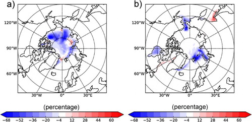
Figure 4.1.2. Ocean heat transports in terawatts (TW; 1 TW = 10¹² watt) derived from GREP (product reference 4.1.1). (a) Modelled net northward ocean heat transport into the Arctic based on monthly averages from the product reference 4.1.1. Grey shading shows the ± one standard deviations as ensemble spread. (b) Zoom-in on 2016. Black line and grey shading shows the 1993–2014 seasonal average with associated ± one standard deviations. Red line shows modelled 2016 heat transport. (c) Similar to (b), but shows the relative contributions to the ocean heat transport from the four openings used to calculate the total net Arctic heat transport.

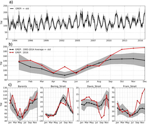
Figure 4.1.3. Maps of anomalies in September 2016 as: (a) Modelled sea-ice concentration (in percentage) from ORAS5 (distributed in product reference 4.1.1). (b) 2 m Atmospheric temperature (in °C) from ERA-interim (product reference 4.1.2). (c) 10 m Wind speed (coloured contours, in m/s) and wind velocity (black arrows) from ERA-interim. Reference climatology is for 1993–2014.

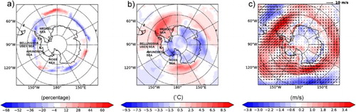
Figure 4.2.1. Location of Argo profiles in the central Labrador Sea during February–March 2016. The colour scale corresponds to the estimated mixed layer depth (in m). The grey line is the 500 m isobath. The black line shows the control box used in Figure 4.2.2. The mixed layer depth is estimated as the depth where the potential density (referenced to 100 m) exceeds the surface value by 0.002 kg/m³ (product reference 4.2.1). The blue square locates Ocean Weather station Bravo.

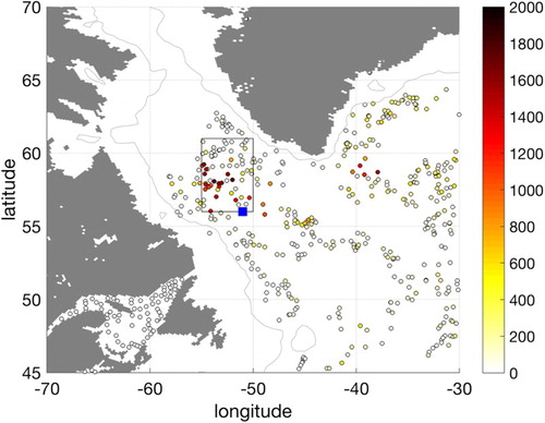
Figure 4.2.2. Upper panel: Depth-time diagram of temperature anomalies (in °C) averaged over the Labrador Sea control box (see Figure 4.2.1) (product reference 4.2.2). The reference period for anomaly computation is the mean over 2003–2014. Lower panel: same for salinity. The monthly temperature optimal analysis fields are averaged over the control box (55–50°W, 56–61°N) and the monthly temperature anomaly field reference is estimated removing their monthly mean over 2003–2014. The black line is the mixed layer depth, estimated as in Figure 4.2.1.

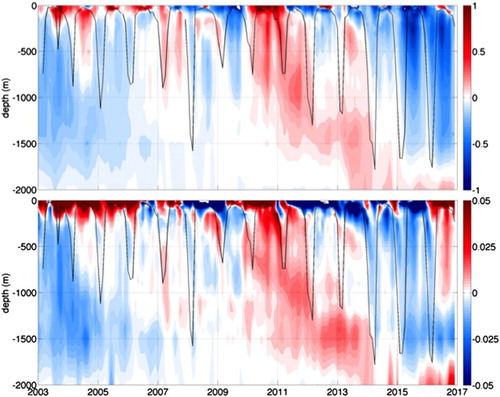
Figure 4.2.3. Top (bottom): April to December 2015 (2016) salinity anomaly integrated vertically from 200 m down to 1000 m (product reference 4.2.2). The reference period for anomaly computation is the mean over 2003–2014. The black line shows the control box used in Figure 2.

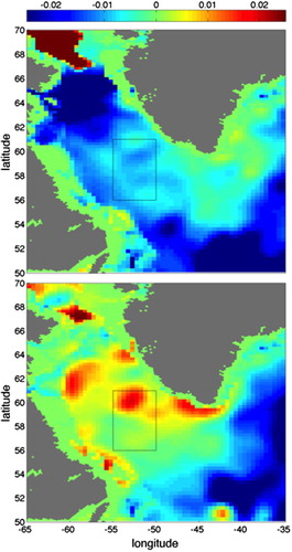
Figure 4.2.4. Top (bottom): mean eddy kinetic energy for 2015 (2016) in m²/s² (product reference 4.2.3)

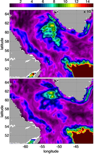
Figure 4.3.1. Top: Temperature anomaly field (in °C) within the 100–400 m depth layer in 2016 (product reference 4.3.1). The reference period for anomaly computation is the mean over 2003–2014. Bottom: same for salinity (in g/kg). The white box corresponds to the control box used in Figure 2 to compute the depth-time diagram.

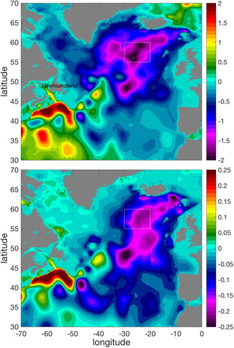
Figure 4.3.2. Top: depth-time diagram of temperature anomalies (in °C) averaged over the control box defined in Figure 4.3.1 (product reference 4.3.1). The reference period for anomaly computation is the mean over 2003–2014. Middle: same for salinity (in g/kg). Bottom: low-pass filtered North Atlantic Oscillation index time series (source: ftp://ftp.cpc.ncep.noaa.gov/wd52dg/data/indices/nao_index.tim).

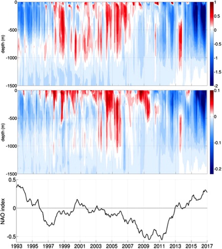
Figure 4.3.3. Location of the 35.1 isohaline estimated from the mean annual salinity field for 2014 (blue), 2015 (green), 2016 (red) and 2003–2014 (black). The black box corresponds to the control box used in Figure 4.3.2 to compute the depth-time diagram (product reference 4.3.1).

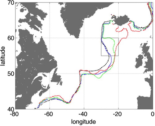
Figure 4.4.1. Map of the positions (colour coded for time) of the floats (a) WMO 6901822 and (b) WMO 6901827 in the South Adriatic Pit. The trajectory of both the floats is confined to the SAP. Sub-figure (c) demonstrated the main circulation scheme of the area. The CMEMS product reference 4.4.1 is used (two Argo float data were selected).

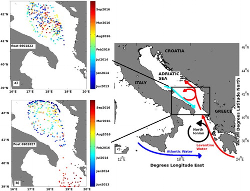
Figure 4.4.2. Hovmöller diagrams of salinity derived from the WMO 6901822 float (upper panel) and WMO 6901827 (lower panel) in the South Adriatic Pit. Temperature (°C) contours are depicted in white over the salinity. Red circles show the two main convection events in 2015 and 2016. The deepening of the LIW during the last four years from about 250 to 700 m (salinity between 38.8 and 38.9) and the intrusion of a salty water mass (salinity larger than 38.9) in the surface–subsurface layer at the end of 2015 are shown in the diagrams.

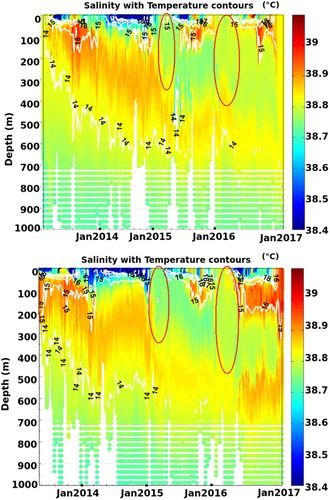
Figure 4.5.1. Seas and locations of tidal gauge stations in the study area of Baltic Sea.

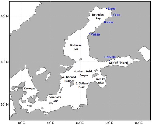
Figure 4.5.2. Sea surface winds at 12GMT in 13 January 2016 from CMEMS Global Ocean Wind L4 Near Real Time product (data sources: product reference 4.5.1).

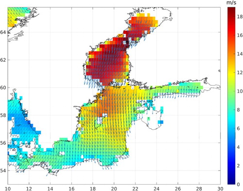
Figure 4.5.3. Hourly sea level at tidal gauge station Kemi in January 2016 (data sources: product reference 4.5.4)

Figure 4.5.4. Sea-ice concentration (%) before and after the storm event in 12–14 January 2016. Left: 14GMT in 12 January 2016; Right: 14GMT in 14 January 2016 (data sources: product reference 4.5.3).

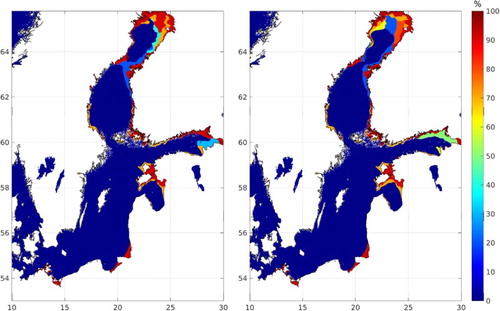
Figure 4.5.5. Monthly minimum sea level (in metre) during January 1978–April 2017 at station Kemi. The five lowest sea level events are indicated with arrows. The blue line shows low sea level with a 20-year return period (data sources: product reference 4.5.4–4.5.5).

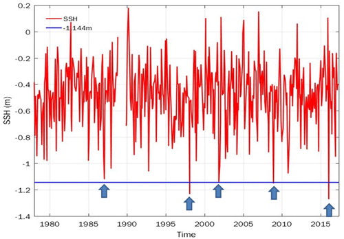
Several regional factors also contributed to the pre-conditioning and maintenance of the Arctic sea-ice anomaly in 2016. The Atlantic Multidecadal Oscillation has remained elevated throughout the 2000s and thus, the temperature of the northward-flowing Atlantic Water is above normal, which is driving negative sea-ice anomalies in the Atlantic sector of the Arctic (Polyakov et al. 2017). The modelled oceanic heat transport towards the Arctic was indeed above average during 2016, especially in fall and early winter (Figure 4.1.2(a,b)). The largest contribution to the heat transport anomaly occurred through the Fram Strait, but anomalously high heat transport was seen also on the Pacific side through the Bering Strait (Figure 4.1.2(c)). Historic sea-ice maps reveal comparable sea-ice extent in the Atlantic sector, most notably the Barents Sea, during a previous period of positive Atlantic Multidecadal Oscillation, e.g. the 1930s (Underhill and Fetterer 2012).

The sea-ice extent in the Barents Sea has been strongly linked to the interannual to multidecadal variations in the oceanic heat transport to the Barents Sea (Sandø et al. 2010; Årthun et al. 2012; Onarheim et al. 2015), that is modulated by temperature anomalies associated with the Atlantic Multidecadal Oscillation (Skagseth et al. 2008; Årthun and Eldevik 2016). 2016 was the warmest year recorded both in the Barents Sea Opening, i.e. the south-western entrance to the Barents Sea, and the interior Barents Sea, as represented by the Kola Section (ICES 2017). This temperature anomaly followed the warm conditions in the upstream Norwegian Sea in 2015 (Larsen et al. 2016), associated with the current, positive phase of the Atlantic Multidecadal Oscillation.

Wind-driven fluctuations in the Barents Sea Atlantic Water throughflow cause coherent ocean heat content anomalies affecting the sea-ice conditions downstream in the interior Barents Sea on timescales up to months (Lien et al. 2013, 2017). Indeed, enhanced low-pressure activity persisted throughout 2016 over the central Barents Sea (ICES 2017), spurring increased Atlantic Water throughflow and subsequent positive ocean heat content anomalies superimposed onto the multidecadal, positive temperature anomaly in the Barents Sea conditioned by the Atlantic Multidecadal Oscillation. Both observations and model results show an anomalous ocean volume and heat transport into the Barents Sea in 2016 (Randi Ingvaldsen, pers. comm.; ICES 2017; Figure 4.1.2(c)), which corroborates the interpretation that an indirectly wind-driven component in 2016 added to the negative anomaly in the sea-ice extent caused by the positive, multidecadal temperature anomaly conditioned by the positive phase of the Atlantic Multidecadal Oscillation.

The Barents Sea has experienced the largest variability in winter sea-ice cover in the Arctic region (Yang et al. 2016), most likely governed by regional driving forces, such as those mentioned above. This variability in sea-ice concentration and extent, and subsequent changes in ocean-to-air heat fluxes have been related to mid-latitude weather patterns in Central Europe, as well as teleconnections to atmospheric pressure systems over the Siberian continent (e.g. Petoukhov and Semenov 2010; Screen et al. 2013; Mori et al. 2014; Schlichtholz 2014, 2016).

Focusing on the Fram Strait region, broad, long-living ice-free areas northeast of Svalbard have been observed in mid-winter in recent years (Ivanov et al. 2015). As in the Barents Sea, the variability of the sea-ice extent northeast of Svalbard is strongly influenced by the characteristics of the inflowing Atlantic Water through the Fram Strait (Polyakov et al. 2017). The variable characteristics are due to propagating anomalies in temperature and salinity generated as far upstream as in the North Atlantic due to Atlantic Multidecadal Oscillation and to the variable strength of the subpolar gyre, regulating the fresh water supply into the Nordic Seas (Hátún et al. 2005). In addition, the atmospheric circulation in the northern Nordic Seas is affecting the ocean circulation on the shorter time scale (Chafik et al. 2015), equivalent to the variability on different time scales as described above for the Barents Sea.

The formation of the strong and re-emerging sea-ice anomalies northeast of the Svalbard archipelago (Figure 4.1.1(b)) has been linked to decreased sea-ice cover during summer, enabling greater influence of oceanic heat on sea-ice from the Atlantic Water deeper below in the water column (e.g. Polyakov et al. 2017). The stronger the heat and freshwater anomalies, the stronger is the influence of Atlantic Water on the sea-ice concentration, and after 2000 there has been a progressive trend of increasing temperature and salinity in the western Nansen Basin northeast of Svalbard, resulting in an upward movement of the thermocline and the halocline.

Furthermore, the variable northward heat transport is a function of variable temperature and volume transports, which again is a function of North Atlantic Oscillation, particularly into the Nordic Seas (Nilsen et al. 2003; Sandø et al. 2012). Hence, the observed sea-ice retreat north of Svalbard in recent winters can be explained by a positive feedback between the decay in summer sea-ice and the growing influence of oceanic heat. For this to happen, several necessary conditions must act jointly to obtain the observed result; depletion of the Arctic Ocean sea-ice extent and ice-free areas northeast of Svalbard, favourable winds in mid-winter, high Atlantic Water inflow and high temperature and salinity of this inflow.

Antarctic sea-ice melted at a pace far faster than ever observed since the onset of satellite sea-ice observations in the early 1980s during the austral summer months of 2016/2017. This resulted in record low values of sea-ice area for each of these months, e.g. sea-ice extent in November 2016 is ∼3.3 Mils km² below the climatological mean (see Figure 1.7.3 in Chapter 1.7), i.e. far outside the previously observed trend and variability.

In the climate scale, a significant correlation between the Nino-3 index and sea-ice extent in the Bellingshausen and Amundsen Seas and the Weddell Gyre has been identified (Yuan and Martinson 2000). The regional distribution and the timing of the Antarctic sea-ice anomalies are also related with the El Niño–Southern Oscillation (ENSO) events (Yuan 2004). Some negative sea-ice extent anomalies were already established in late 2015, suggesting teleconnections between Antarctic sea-ice anomalies and the 2015/2016 El Niño event. Map of ORAS5 (Zuo et al. 2017, 2018) sea-ice concentration anomalies in September 2016 shows a distinct asymmetric pattern (Figure 4.1.3(a)) which travelled around the continent and has developed since southern fall. This is associated with atmospheric zonal wave three pattern (Raphael 2004). This atmospheric circulation pattern can transfer extra poleward (warmer) flow from the sub-tropics and is believed to influence the sea-ice extent mostly in the southern fall and early winter (Raphael 2007).

The temperature difference between the atmosphere and the ocean affects the transfer of sensible heat, which could be reflected in regional growth or melt of the sea-ice. A map of atmospheric 2 m temperature anomalies from ERA-interim (Dee et al. 2011) for the same month suggests that the negative sea-ice concentration anomalies are normally aligned under regions with a positive atmospheric temperature anomaly (Figure 4.1.3(b)), e.g. in the Bellingshausen Sea and Weddell Gyre, and sectors bordering the western Indian Ocean and parts of the Pacific between 130° and 200°E. Regional forcing such as surface winds and ocean currents can also drive movement of sea-ice, to a region where it would either melt or accumulate. Thin sea-ice is more susceptible to dispersion or compression by winds. The strong reduction of sea-ice extent in September 2016 at the Bellingshausen Sea and Weddell Gyre is associated with the anomalously strong north-westerly winds in the Atlantic sectors (Figure 4.1.3(c)), and subsequently related to the positive sea-ice concentration anomalies in the eastern Atlantic Ocean sector. Similar anomalous north-westerly winds in the Pacific sector also enhanced the Antarctic sea-ice lost between 130° and 200°E.

The mean ocean current and relative long memory of ocean heat content also play an important role in the advection of sea-ice anomalies and predictability of sea-ice extent (Holland et al. 2013). The strong negative Antarctic sea-ice extent anomalies developed in the last three months of 2016 (Figure 1.7.3(b)) were likely pre-conditioned by a persistent positive surface heat flux anomaly in the ocean throughout the year (Tietsche et al. 2017).

4.2. Deep convection in the Labrador Sea

Leading authors: Julie Deshayes, Jérôme Gourrion

Contributing authors: Mélanie Juza, Tanguy Szekely, Joaquín Tintore

Statement of outcome: Deep convection has been monitored in the central Labrador Sea in winter 2016, followed by positive salinity anomalies at 200–1000 m depth presumably due to intensified turbulent salt fluxes from the boundaries. The latter contrasts with 2014 and 2015, when deep convection also occurred but was followed by negative salinity anomalies in the central Labrador Sea.

Products used:

Table

Ref. no.	Product name and type	Documentation
4.2.1	INSITU_GLO_TS_REP_OBSERVATIONS_013_001_B In situ	PUM: http://marine.copernicus.eu/documents/PUM/CMEMS-INS-PUM-013-001-b.pdf QUID:http://marine.copernicus.eu/documents/QUID/CMEMS-INS-QUID-013-001b.pdf
4.2.2	INSITU_GLO_TS_OA_REP_OBSERVATIONS_013_002_B In situ	PUM: http://marine.copernicus.eu/documents/PUM/CMEMS-INS-PUM-013-002-ab.pdf QUID: http://marine.copernicus.eu/documents/QUID/CMEMS-INS-QUID-013-002b.pdf
4.2.3	SEALEVEL_GLO_PHY_L4_REP_OBSERVATIONS_008_047 Remote sensing	PUM: http://marine.copernicus.eu/documents/PUM/CMEMS-SL-PUM-008-032-051.pdf QUID: http://marine.copernicus.eu/documents/QUID/CMEMS-SL-QUID-008-032-051.pdf

The North Atlantic basin hosts the unique northern hemisphere deep convection regions where most dense water is formed, supplying the deep limb of the Atlantic Meridional Overturning Circulation (AMOC). The latter, controlled by a variety of processes worldwide (Kuhlbrodt et al. 2007), in turn controls the ocean's capability to store heat and anthropogenic carbon. European climate variability is strongly regulated by fluctuations in the intensity and extent of AMOC. While direct observations of the AMOC are limited, monitoring fluctuations of deep convection in the North Atlantic may be useful to picture past, present and future changes in the AMOC. Nevertheless, the North Atlantic is an area with strong ocean-ice–atmosphere interactions, high interannual and decadal variability and its long-term changes in temperature and salinity over the last century are still a matter of debate. After a monotonic decrease of winter convection intensity (often suggested as an indicator of AMOC slowing down) since the mid-1990s (Yashayaev and Loder 2016), intense convection has been reported since 2014. It still remains to be understood if the AMOC intensity is actually decreasing at multidecadal time scales (Terray 2012) or is directly controlled by fluctuations in the Labrador Sea deep convection. In order to contribute to the debate, this section provides an insight on the recent Labrador Sea convective activity and the associated anomalies in hydrographic properties at intermediate depth.

Several Argo profiles have monitored mixed layer deeper than 1000 m in February–March 2016 in the central part of the Labrador Sea, with some values reaching 2000 m and beyond (Figure 4.2.1). The deepest profiles are in the vicinity of Ocean Weather station Bravo where convection was historically detected (Lilly et al. 1999). Newly formed Labrador Sea Water is cooler than surrounding water masses, hence the negative temperature anomalies seen in the depth-time Hovmöller diagrams after 2014 (Figure 4.2.2, top panel). An extended version of this figure (not shown) suggests that convection in 2016 actually reached levels observed before 1995. This illustrates the magnitude and significance of interannual to decadal-scale variations in the Labrador Sea. Consequently, deriving long-term trends of hydrographic properties in that region requires comprehensive observations with high-frequency space and time sampling rates.

Contrasting with temperature observations, the salinity anomalies at 200–1000 m depth in the central Labrador Sea, which are negative in 2014 and 2015, become positive in 2016 after the mixed layer has shoaled back to the surface (Figures 4.2.2 and 4.2.3). According to previous studies (Lilly et al. 2003; Straneo 2006; Chanut et al. 2008), the post-convective phase is characterised by lateral turbulent fluxes in between the central Labrador Sea and the surrounding boundary currents, particularly the West Greenland Current to the southwest of Greenland. Hence the positive salinity anomaly in 2016 presumably comes from increased turbulent salt fluxes at depth in the central Labrador Sea.

Turbulent fluxes of tracers in the upper ocean are related to the level of surface eddy kinetic energy. Thus, the increase in turbulent fluxes that presumably happened in 2016 in the Labrador Sea should be detected via an increase in eddy kinetic energy. However, eddy kinetic energy in the Labrador Sea derived from altimetry was of similar intensity in 2014 (not shown), 2015 and 2016 (Figure 4.2.4). In order to solve this contradiction, it could be argued that the turbulent fluxes of salt in between the central Labrador Sea and the surrounding boundary currents are achieved by three types of eddies, of which only one, namely the Irminger rings, is large enough to be detected by altimetry at this latitude (Chanut et al. 2008). As a result, the absence of an anomaly in eddy kinetic energy in 2016 as derived from altimetry cannot be used to repudiate the hypothesis that turbulent salt fluxes have increased at the same time.

Turbulent fluxes of heat and salt in the Labrador Sea are produced by the mixed barotropic-baroclinic instability of the boundary currents (Katsman et al. 2004). Hence, their intensity depends on boundary current strength, vertical structure and horizontal gradients in density in between the boundary current and the central Labrador Sea. In 2016, positive salinity anomalies are found at depth (200–1000 m) in the boundary currents of Labrador Sea (Figure 4.2.3): to the south of Greenland, in the north-west, and along the Labrador Current, which supports the hypothesis of increased turbulent salt fluxes in 2016. At the surface, a similar positive anomaly is observed in the East and West Greenland currents (see Figure 1.3.1). The positive salinity anomaly in the central Labrador Sea (53°W, 60°N) as visible in the Hovmöller diagram (Figure 4.2.2) is presumably a consequence. Several mechanisms may be responsible for salinity anomalies in Labrador Sea boundary currents at depth, among which [i] anomalies in freshwater input from the Arctic and Nordic Seas via the East Greenland Current, and [ii] anomalies in the penetration of salty subtropical water masses in the eastern subpolar gyre. Both may be related to the strength and shape of the cyclonic subpolar gyre circulation, ultimately influenced by dense water formation in the Labrador Sea. Hence, it is possible that the intensified convection in 2014–2015 has contributed to the positive anomalies seen in the central Labrador Sea at depth in 2016.

Finally, it is important to mention that convection in the Labrador Sea is not isolated from convection in the Irminger Sea (Deshayes et al. 2007), hence a detailed analysis of recent convective events in the subpolar gyre should encompass both regions. Besides, it remains an open question whether the AMOC time series, as derived from direct observations, indirect products (e.g. altimetry) and/or ocean reanalyses, reflect the observed time series of convection in the subpolar gyre.

4.3. A persisting regional cold and fresh water anomaly in the Northern Atlantic

Leading authors: Jérôme Gourrion, Julie Deshayes

Contributing authors: Mélanie Juza, Tanguy Szekely, Joaquín Tintore

Statement of outcome: A regional cold and fresh anomaly in the North Atlantic, strengthening since late 2013, has been observed in 2016. It is suggested that the physical explanation of this event cannot be based only on air–sea fluxes but should also account for the modification of the subpolar gyre dynamics such as the circulation intensification and the eastward migration of its eastern boundary during repeated winters with North Atlantic Oscillation index increasing strongly over a few years.

Products used:

Table

Ref. no.	Product name and type	Documentation
4.2.1	INSITU_GLO_TS_REP_OBSERVATIONS_013_001_B In situ	PUM: http://marine.copernicus.eu/documents/PUM/CMEMS-INS-PUM-013-001-b.pdf QUID:http://marine.copernicus.eu/documents/QUID/CMEMS-INS-QUID-013-001b.pdf

While the global ocean temperatures in the last decade are the warmest ever observed since modern record keeping, a regional ‘cold blob’ pattern has been observed in 2014 in the North Atlantic near 55°N, 30°W (NASA 2016), growing in 2015 (Henson 2016) and persisting in 2016 (Ortega 2017). Using the global CMEMS in situ observation reprocessed dataset (product reference 4.3.1), it is shown that such a cold anomaly is accompanied by anomalously fresh water with similar spatial pattern (Figure 4.3.1). These signatures appear from 40°W to 15° W and from 45°N to 60°N, which sits within the eastern part of the subpolar gyre and around the North Atlantic Current (e.g. Bower and von Appen 2008). From the surface to 1000 m depth, these cold and fresh anomalies exceed 1°C and 0.2 g/kg in 2016 (Figure 4.3.2).

Besides the low occurrence of such intense anomalies in the climatic-scale time series, these extreme events are located in an oceanic area of particular importance since it is the pathway of the poleward meridional heat transport that controls the northern temperate Earth climate. Moreover, at interannual scale such anomalies alternate with warm and salty ones, their pattern is very similar with that of the linear temperature trend over the twentieth century (Rahmstorf et al. 2015), suggesting that they are getting more frequent and/or intense.

Similar events of large fresh and cold anomalies have already been reported in the literature, named as the Great Salinity Anomalies in the 1970s (Dickson et al. 1988; Belkin et al. 1998), 1980s and 1990s. They occurred over time periods with persistent and positive winter North Atlantic Oscillation index, i.e. during atmospheric conditions of intensified westerly winds leading to increased ocean heat loss and eastward water mass transport. The fresh and cold waters can be of remote origin from the Arctic basin and transferred to the Labrador Sea through the Canadian archipelago. Under positive North Atlantic Oscillation index conditions, positive sea-ice extent anomaly systematically appears (Drinkwater 1994; Prinsenberg et al. 1997), leading to increased negative temperature and salinity anomalies east of Newfoundland within 1–2 years (Deser and Timlin 1996). Aagaard et al. (1996) have shown that the additional volume of Arctic sea-ice export through Fram strait in the early 1970s was large enough to explain the exceptional intensity of the 1970's Great Salinity Anomaly. Beyond the contribution of the remote Arctic waters, a recurrent source of cold and fresh water at depth in the southern Labrador Sea is localised through deep convection events in the central Labrador Sea basin (see Section 4.2). Once the anomalies were generated, they were advected eastwardly up to the Barents Sea 8–10 years later for the 1970s’ Great Salinity Anomaly, and 6–7 years for 1980s’ and 1990s’ ones, suggesting a change in the advection velocity likely explained by an intensification of the gyre circulation (Belkin 2004). Several authors have also suggested that the persistence of such anomalies might be explained by a 300–400 km eastward shift of the eastern boundary of the subpolar gyre (Ellett and McDougall 1983; Dooley et al. 1984; Martin et al. 1984).

The causes of rapid warming of the North Atlantic subpolar gyre during the 1990s have been analysed in Robson et al. (2012). The pre-1995 period is characterised by a prolonged positive North Atlantic Oscillation phase (Figure 4.3.2, bottom panel), with temperature anomalies in the upper subpolar gyre negatively correlated with the atmospheric index and maximum correlations found when the index leads by one year. As the atmospheric index reaches its peak value in the early 1990s, a large layer of anomalously cold water is formed in the Labrador Sea (Yashayaev et al. 2007) through increased deep convection, particularly in the years 1990–1993 (Lazier et al. 2002). During the winter 1995–1996, the upper subpolar gyre warms rapidly, coincidently with unusually low North Atlantic Oscillation index. In contrast, with the previous period, while the index returns to near neutral levels, the positive heat content anomalies persist and are not simply responding to the concurrent or previous year’s atmospheric conditions, suggesting that some other mechanism influences the relationship between the North Atlantic Oscillation and ocean heat content. Robson et al. (2012) concluded that the spatial pattern of heat content anomalies cannot be driven only by the surface heat fluxes and likely results from a dynamic change in the ocean circulation forced by anomalous buoyancy fluxes. As a result of a cold subpolar gyre in the early 1990s, the meridional density gradient between subtropical and subpolar gyres is anomalously high, leading to a particularly intense circulation of both gyres; the authors showed how the subpolar gyre barotropic stream function anomaly peaks in 1994, indicating an acceleration of the gyre circulation after a few years of positive North Atlantic Oscillation index, before decreasing to negative values coinciding with the warming event. They also showed that the Atlantic Meridional Overturning Circulation strength anomaly at 45°N, close to 1 Sv in the early 1990s, peaks to 3 Sv just before the warming event in their simulation. They concluded that the warming event is led by the ocean heat transport convergence and amplified by the westward displacement of the eastern subpolar gyre boundary. The wind forcing contributes but is not the primary cause.

Lagrangian drifter and altimetry data have been used over the period 1992–1998 to compare circulation changes between years with positive (1992–1995) and negative (1995–1998) North Atlantic Oscillation index (Figure 4.3.2, bottom panel) (Flatau et al. 2003). The positive index years were associated with a strengthening of the eastward flow, making the eastern subpolar front sharper and located farther east. Diagnosing that the air–sea heat flux does not explain the sea surface temperature changes, it was suggested that cooling in this region may be explained by changes in sea surface temperature advection (i.e. anomaly) and an eastward shift in the North Atlantic Current location (Bower and von Appen 2008). Using the 7°C and 8°C isotherms as rough indicators of North Atlantic Current axis, the authors observed their eastward displacement during positive North Atlantic Oscillation years.

Using simulations, Hátún et al. (2005) focused on the gyre shape to understand its impact on the thermohaline circulation during the 1990's Great Salinity Anomaly. Considering the 35.1 isohaline as an indicator of the subpolar gyre boundary, they found that the transition from cold/fresh to warm/salty anomalies in the 1990s was accompanied by a westward displacement of the eastern subpolar gyre edge.

Since the extension/contraction of the subpolar gyre might be crucial in maintaining such anomalies, the location of the eastern boundary of the subpolar gyre for the recent period is estimated using the 35.1 isohaline (Figure 4.3.3), as done by Hátún et al. (2005). The results suggest that, jointly with the intensification and propagation of the present cold/fresh anomaly, the eastern boundary of the subpolar gyre has been recently migrating eastward from 2014 to 2016 by about 1000 km.

In order to address the possible relation with the gyre circulation variations, Hakkinen and Rhines (2004, 2009) used altimetry and Lagrangian drifter trajectories during the 1990s to characterise a change in the near-surface current pattern accompanying a transition from warm/salty anomalies and low North Atlantic Oscillation index to cold/fresh ones and high index. They showed that such a transition is associated with a strengthening of the gyre and a northeastward flow acceleration in the subpolar gyre in its eastern part.

Frankignoul et al. (2009) compared two extreme opposite periods in terms of temperature and salinity anomalies and North Atlantic Oscillation index using simulations to investigate the variability of the Atlantic Meridional Overturning Circulation. During 1973–1977, the atmospheric index was predominantly positive and the subpolar front in an eastward position, restricting the salty subtropical waters to the region east of 20°W in the eastern subpolar domain; by contrast, in 1998–2002 when the index had retreated to a negative or neutral phase, the subpolar front was retracted westward, and the salty subtropical waters extended further into the subpolar basins. They found that, following a positive phase, the Atlantic Meridional Overturning Circulation intensifies due to the gyre acceleration, but the associated northward salt transport does not; indeed, the acceleration of the North Atlantic Current is compensated by the inter-gyre boundary migration and the overall transport is not modified.

Finally, the 2016 temperature and salinity anomalies in the mid-latitude North Atlantic can be described in the light of the above description of past similar events, i.e. as a delayed consequence of a rapid change of the North Atlantic Oscillation index. Analogy with the Great Salinity Anomalies from the past decades, i.e. similar transition from low to high index values in the 1970s or opposite changes during the 1990s, is used to analyse the present situation. Past events analysis suggests that a rapid adjustment to local anomalies of air–sea heat or horizontal freshwater fluxes is not sufficient to explain both the vertical distribution of the observed anomalies and their temporal persistence. Due to the increased meridional temperature and salinity gradients, the subpolar and subtropical gyres as well as the North Atlantic Current are accelerated, leading to increased meridional mass transport; nevertheless, the eastward migration of the gyre boundary brings a compensatory effect that allows the overall meridional heat and salt transports to be maintained.

It is proposed that a regional adjustment of the basin-scale dynamic structures is likely responsible for the present thermohaline variations observed since 2014. Anomalies at the boundaries of the present area of interest can be interpreted on the basis of the same dynamic modifications (see Section 4.2 on the convection in the Labrador Sea). Similar considerations suggest that in the coming years, we might observe the propagation of the present anomalies further northward. In the context of the present report on the 2016 ocean state at global scale, other possible contributing mechanisms are not detailed here as the literature on similar past events suggests that they cannot explain the vertical distribution and temporal persistence of such observed anomalies.

4.4. Unusual salinity pattern in the South Adriatic Sea in 2016

Leading authors: Zoi Kokkini, Giulio Notarstefano

Contributing authors: Pierre-Marie Poulain, Elena Mauri, Riccardo Gerin, Simona Simoncelli

Statement of outcome: A double maximum salinity pattern has been observed since the late 2015 in the South Adriatic Sea. The first maximum is located in the near-surface layer at the depth of about 50 m with salinity larger than 38.9 and the second at about 400–500 m with salinity of about 38.8, which is traditionally considered as the Levantine Intermediate Water. The winter convection of 2016 led to a more homogeneous water column but these saline veins continued flowing in the South Adriatic even after the convection and throughout 2016, maintaining this double salinity maximum. Our study hypothesised that the Adriatic–Ionian bimodal oscillating system is one of the factors that contributes to this double salinity maximum pattern by feeding the Adriatic with this saline vein. Due to the importance of the South Adriatic as a fundamental source of dense water for the Eastern Mediterranean Sea, the continuous monitoring of such pattern changes could help in thermohaline circulation studies in the area.

Products used:

Table

Ref. no.	Product name and type	Documentation
4.4.1	INSITU_MED_NRT_OBSERVATIONS_013_035 In situ	PUM: http://cmems-resources.cls.fr/documents/PUM/CMEMS-INS-PUM-013.pdf QUID: http://cmems-resources.cls.fr/documents/QUID/CMEMS-INS-QUID-013-041.pdf

A particular salinity pattern is observed since the end of 2015 in the South Adriatic and characterised by a double salinity maximum. Data are mainly used from Argo floats during the period 2013–2016 (floats WMO 6901822 and WMO 6901827, see Figure 4.4.1 for details on data). The first maximum (and with the stronger signal centred at about 50 m depth) is located in the near-surface layer and the second at about 400–500 m, which is traditionally considered as the Levantine Intermediate Water (Giorgetti 1999). We speculate about its origin and find a possible connection with the upper-layer circulation in the North Ionian Sea. This circulation mechanism, called the Adriatic–Ionian bimodal oscillating system (Gačić et al 2011), drives the Northern Ionian circulation reversal from cyclonic to anticyclonic and strongly affects the distribution of salt in the South Adriatic (Gačić et al. 2010, 2011). The South Adriatic is also one of the site of deep water convection in the Mediterranean Sea and a fundamental source of dense water for the Eastern Mediterranean (Demirov and Pinardi 2002), as presented in Section 3.4 of this issue. For this reason, the area is an important site that is continuously monitored with several oceanographic platforms, like profiling floats and gliders. These mobile autonomous platforms provide a huge amount of profiles which give the opportunity to study new and existing features.

Two Argo floats (see Figure 4.4.1 for details on data) were operating continuously inside the South Adriatic Pit since 2013. The analysis of the salinity revealed interesting haline characteristics for these years and mainly for 2016. The floats were trapped by the South Adriatic cyclone and remained in the area, leading to a continuous monitoring of its thermohaline properties. The floats remained in the Pit until the end of 2016, when one of them exited from the Otranto Strait (their positions in time are showed in Figure 4.4.1). These float data depicted well the seasonal and the spatial variability of the thermohaline characteristics of the area.

Here, we focus on the analysis of the salinity data which are presented in the Hovmöller diagrams (Figure 4.4.2). The seasonality is depicted for most of the years. The surface waters are getting warmer and lighter and this drives stratification and the creation of the thermocline in the South Adriatic Pit. The salinity follows the temperature profile and the stratification remains until October–November of every year, when it starts to get weaker and eventually breaks during the convection events that are taking place in the end of February and driving to the mixing of the water column. This mixing is visible, sometimes, down to 400 m or deeper (as it happened in winter 2013 with a convection event deeper than 500 m), depending on the intensity of each convection episode and the severity of the winter. The convection events led to the deepening of the Levantine Intermediate Water in the South Adriatic Pit during the last four years. At the end of summer 2013, the salinity maximum was placed around 250 m and it was at about 38.9, much higher than the expected value for the entering Levantine Intermediate Water. In 2014, this maximum went deeper than 300 m and in 2015 it was found at about 500 m depth. Meanwhile, at the end of 2015 an intrusion of a salty water mass in the near-surface layer was observed by the two floats. It was characterised by a salinity higher than 38.92 and it was placed in the first 100 m, while the existing ‘old’ Levantine Intermediate Water continued deepening. This intrusion resulted to an abnormal salinity pattern in the South Adriatic Pit. The water column is now characterised by a double salinity maximum. The first one is placed in the first 100 m and it is the saltier one (S _P > 38.9) while the second is extended from 400 m to almost 700 m (S _P ∼ 38.8), while the layer in between them has an intermediate salinity (S _P ∼ 38.7). The convection in the end of February 2016 led to the mixing of the water column with an increased salinity, as observed also in the entire Mediterranean Sea down to 500 m (see Section 1.4). The saline vein continued entering in the South Adriatic after the convection and for the whole 2016, maintaining this double salinity maximum.

We can hypothesise that the inversion of the Adriatic–Ionian bimodal oscillating system from anticyclonic to cyclonic mode after 2011 contributed to the salinification of the South Adriatic Pit in 2016 by limiting the Atlantic water from entering in the area and boosting the surface saline waters advected from the eastern Ionian Sea on their pathway to the Adriatic Sea (Gačić et al. 2011). The aforementioned particular circulation alongside, together with other factors that could be predominant in the area, such as river discharges and meteorological conditions, could have led to the creation of this double salinity pattern. The saline evolution of the South Adriatic should be carefully monitored because it is an important site of deep water convection (Zore-armanda 1969, 1972; Demirov and Pinardi 2002) in the Mediterranean Sea and a fundamental source of dense water for the Eastern Mediterranean Sea (see also Section 3.4 of this issue). The aforementioned changes in the thermohaline pattern of the South Adriatic Pit may be indicative of the contribution of other factors, probably underestimated until now. Our ongoing work focuses on investigating the impact of these factors (such as river discharges and meteorological condition) on the thermohaline pattern and circulation of the South Adriatic area.

4.5. Extremes of low sea level in the Northern Baltic Sea

Leading author: Jun She

Contributing author: Viktorsson Lena

Statement of outcome: A new record of low sea level since 1922 was observed at the Bothnian Bay station Kemi. This low sea level is caused by a storm with strong northeasterly winds. It is found that there is a significant increase of extreme low sea level events in 1998–2016 in comparing with period of 1978–1997. The potential relation between low sea-ice extent and the extreme low sea level in the Bothnian Bay is discussed. It was also found that, in order to correctly forecast this event, it is important to predict the ice condition correctly in the model.

Products used:

Table

Ref. No.	Product name & type	Documentation
4.5.1	WIND_GLO_WIND_L4_NRT_OBSERVATIONS_012_004 Remote sensing	PUM: http://marine.copernicus.eu/documents/PUM/CMEMS-OSI-PUM-012-004.pdf QUID: http://marine.copernicus.eu/documents/QUID/CMEMS-OSI-QUID-012-004.pdf
4.5.2	BALTICSEA_ANALYSIS_FORECAST_PHY_003_006 Model	PUM: http://marine.copernicus.eu/documents/PUM/CMEMS-BAL-PUM-003-006.pdf QUID: http://marine.copernicus.eu/documents/QUID/CMEMS-BAL-QUID-003-006.pdf
4.5.3	SEAICE_BAL_SEAICE_L4_NRT_OBSERVATIONS_011_004 Remote sensing	PUM: http://marine.copernicus.eu/documents/PUM/CMEMS-OSI-PUM-011-004.pdf QUID: http://marine.copernicus.eu/documents/QUID/CMEMS-OSI-QUID-011-004.pdf
4.5.4	INSITU_BS_TS_REP_OBSERVATIONS_013_042 In situ	PUM: http://marine.copernicus.eu/documents/PUM/CMEMS-INS-PUM-013-042.pdf QUID: http://marine.copernicus.eu/documents/QUID/CMEMS-INS-QUID-013-042.pdf
4.5.5	INSITU_BS_NRT_OBSERVATIONS_013_034 In situ	PUM: http://marine.copernicus.eu/documents/PUM/CMEMS-INS-PUM-013-042.pdf QUID: http://marine.copernicus.eu/documents/QUID/CMEMS-INS-QUID-013-042.pdf

Very low sea level in the Baltic Sea may cause small harbours to fall dry and may cause severe problems for navigation. In the Northern Baltic Sea, such events are often generated by storms with strong offshore winds (Wolski et al. 2014). During the past 20 years (before 2016), storms have caused extreme low sea level events in the north-eastern Baltic Sea coast in 31 January 1998 and 28 January 2010 (Wolski et al. 2014). The 1998 storm generated record low sea level of −1.24 m at station Kemi (Figure 4.5.1) since 1922 while the 2010 storm mainly affects the Gulf of Finland, generating the record low sea level in Helsinki since 1904 (−0.93 m). In 2016, a new low sea level of −1.28 m was recorded at the station Kemi, due to a strong storm affecting the northern Baltic Sea during 12–14 January 2016.

The storm affects the region from 18GMT on the 12th of January 2016 with northeasterly winds of 12–14 m/s, prevailing in the northern Baltic Sea. The winds increase to 20 m/s at 12GMT in 13 January (Figure 4.5.2). The water level at Kemi reaches −1.28 m in the morning of 14 January 2016 (Figure 4.5.3), which is the lowest sea level ever observed at Kemi and also the third lowest sea level in the Finnish coast ever recorded since 1904. The previous records are −1.29 m at Raahe station and −1.31 m at Oulu station, both in 1922. The storm in January 2016 also causes low sea level at other Finnish stations, e.g. Oulu (−1.10 m), Raahe (−1.12 m) and Vaasa (−0.71 m).

The presence of sea ice would inevitably affect the sea level in the storm case. If the water surface is covered by a significant amount of sea ice, the momentum flux into the water will be closely linked to the sea-ice extent, density and drift velocity. In order to give right sea level in icing waters, tt is essential for the forecasting models to predict both the sea level dynamics and the sea-ice conditions. This can be quite challenging to the ocean-ice forecast models as it is difficult to in correctly resolve full ice rheology in the model. This issue is investigated in the 2016 storm. The sea-ice concentration right before and after the storm is shown in Figure 4.5.4. A comparison with daily Bothnian Bay sea-ice coverage climatology during 1978–2016 shows that the sea-ice concentration in 12 January 2016 is slightly lower than climatology (Figure 4.5.4, left). The further decreased sea-ice concentration after the storm (Figure 4.5.4, right) suggests that the storm leads to intense dispersion of the sea ice.

The importance of the sea-ice state in the Baltic Sea during the lowest sea level event is also shown in CMEMS model results but in a different way. It was found that CMEMS model forecast in the Baltic Sea missed this event as the model predicted much more sea ice than the observations during 12–14 January 2016 (not be shown here).

Another question is whether there are significant climate change signals on the low sea level events. Figure 4.5.5 displays the time series of monthly minimum sea level at Kemi during January 1978–April 2017. Based on extreme sea level analysis using tidal gauge observations in 1960–2010, it was found that the low sea level with a 20-year return period is −1.14 m at Kemi (Wolski et al. 2014). Figure 4.5.5 shows that, during 1998–2017, there are four events reach or exceed this level, while no low sea level event reaching the 20-year return period was recorded during the period 1978–1997. This suggests that the extreme low sea level events in the Bothnian Bay occur much more frequently during the last 20 years. Further investigation shows that the two of them happen in November (2001 and 2008) with almost free sea-ice condition as November is the very beginning of the sea-ice season. The other two events, in January 1998 and January 2016, are in the normal sea-ice extent comparing to the normal years. This suggests that the extreme low sea level events in the Bothnian Bay tend to coincide with winters with normal or less sea-ice coverage.

Over the past 100 years, significant climate warming and increasing sea-ice melt have been detected (HELCOM 2013). During the past 30 years, the trend of sea surface temperature in the Bothnian Bay has reached 1°C/decade, which is the largest warming in the entire Baltic Sea. The sea-ice coverage in the Baltic Sea has decreased by 20% as well as the length of the sea-ice season which has been reduced by 18 days over the past 100 years. It is speculated that the increasing sea-ice melt in this region may be in favour of occurrence of the low sea level events in the Bothnian Bay. However, this may not be the main reason for the increasing number of low sea level events in the past 20 years. Changes in storm directions, frequencies and strength may also lead to such variations. It should be noted that the reasons for low sea level events in the Bothnian Bay are complicated and may not all be caused by storms and in related to the low sea-ice extent. One example is the low sea level (−1.12 m) recorded on 26 January 1987 at Kemi when the Bothnian Bay and Bothnian Sea are almost fully covered by sea ice. There were also no particular strong local winds blowing during this particular event. In 26 January 1987, heavy sea ice covers the Bothnian Bay and eastern part of Bothnian Sea. In Bothnian Bay and Bothnian Sea, calm weather prevails before 06GMT 25 January. The winds turn to northerly and becomes relatively strong (12–16 m/s) in the rest of the day and first half of 26 January (figures are not shown). In the central Baltic Sea, strong north-westerly winds prevail (>16 m/s). Such wind pattern can drive the waters in Bothnian Sea southward which may be one of the reasons for the low sea level at Kemi in 1987. Detailed mechanism of the low sea level event in 1987 needs further modelling investigations, which is not done in this paper. The above results strongly underline the need for in-depth exploration of atmosphere–ocean-ice interaction and basin-scale transport in the role of forming the low sea level events in the northern Baltic Sea.

Chapter 5 – Synthesis

5.1. Long-term changes

Ocean temperatures have been increasing during the past two decades (1993–2016) at a global scale and particularly in the European regional seas. The global ocean warms at a rate of +0.8±0.1 W/m². Accordingly, we estimate a current Earth Energy Imbalance of +0.7 W/m² over the ‘golden’ period 2005–2016 (i.e. when best sampling coverage of the global ocean observing system is available). In the European regional seas, the rates of mean sea surface temperature trends during the past 24 years are particularly strong (Figure 5.1.1). Upper ocean (0–700 m) warming rates in the regional seas range from +0.6±0.1 W/m² in the Arctic area up to +1.3 ±0.1 W/m² in the Mediterranean Sea. Mean sea level has been rising during the period 1993–2016 at a global rate of +3.3 mm/year, and about one-third of this rise is driven by ocean warming. In the European regional seas, sea level rates range from +2.6 (North West Shelf) up to +4 mm/year (Baltic Sea, Figure 5.1.1).

Both the sea ice volume and extent have shown concomitant long-term changes in the northern and southern hemisphere polar regions and in the Baltic Sea. In the Arctic, sea ice extent decreased at a rate of −0.78 × 10⁶ km² per decade over the period 1993–2016 which corresponds to a decrease of 6.15% per decade (Figure 5.1.1). Arctic sea ice loses volume at a rate of 15.4% per decade over the past 24 years. Arctic Ocean freshwater content increased since the mid-90s which is linked to the reported sea ice volume change. In the Antarctic, sea ice extent increased by 1.6% per decade and by 8.8% per decade for sea ice volume over the period 1993–2016.

Important changes in the North Atlantic area have been reported as well. During the past 24 years, the Gulf Stream decelerated. Deep penetrating (∼1000 m) year-to-year temperature and salinity changes prevailed in the subpolar North Atlantic during the period 1993–2016 and persist over three to five years, with fundamental impact on the hydrographic conditions in this region. The Atlantic Meridional Overturning Circulation showed considerable variability on monthly and interannual timescales over the period 1993–2016, and its strength weakened since about the year 2005, which is driven by long-term variability rather than an ongoing trend.

Western boundary current systems show spatial displacements and changes in current strength over the 1993–2016 study period. In the North Pacific, the Kuroshio is currently in a stable mode but shifted northward. In the southern hemisphere, both the Malvinas current and Agulhas current branch decelerated, and the latter shifted southward. The Tasman front decelerated over the 1993–2016 study period.

Chlorophyll-a, the main photosynthetic pigment contained in all phytoplankton, has shown significant trends during the past 18 years (1998–2016). In high latitudes, chlorophyll-a showed an increasing trend, whereas, in the tropical areas a decreasing trend is observed. The previously reported expansion of ocean biological deserts in the North Pacific subtropical gyre areas decelerated over the past decade, and even reversed in the North Atlantic and South Pacific. However, given the length of the chlorophyll-a time series (less than two decades), these results have to be seen as evidence of climate variability during the study period, rather than as evidence of climate change. In the European regional seas, chlorophyll-a trend was positive over the same period, with the exception of the Black Sea. In this European regional sea, however, the vertical extent of the Black Sea oxygenated layer narrowed from 140 to ∼70 m during the past 60 years, following a deoxygenation trend recently intensified by anthropogenic atmospheric warming.

Figure 5.1.1. Schematic overview on trends over the 1993–2016 (black) and 2005–2016 (blue) periods. More details are given in the text, and information on uncertainty estimates can be found in the corresponding sections, respectively. Abbreviations: GLOB, global ocean; MED, Mediterranean Sea; IBI, Iberia-Biscay-Ireland; NWS, North West Shelf; BS, Black Sea; BAL, Baltic Sea.

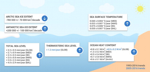
Figure 5.2.1. Schematic overview on anomalous changes taking place in the marine environment during the year 2016. Upward arrow indicates anomalous positive values, downward arrow indicates anomalous negative values, and the star points to deep convection events. Abbreviations: SSS, sea surface salinity; SST, sea surface temperature; T, subsurface temperature; S, subsurface salinity; OHC, ocean heat content; SL, – sea level; CO2, sea-to-air CO₂ flux; CHL-a, chlorophyll-a; CUR, surface currents; MTH, meridional heat transport; ITF, Indonesian Throughflow; NI, nitrate; Sea ice, sea ice extent.

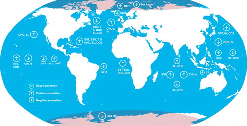
Figure 5.2.2. Schematic overview on anomalous changes taking place in the European regional marine environment during the year 2016. Upward arrow indicates anomalous positive values, downward arrow indicates anomalous negative values, a cross means ‘no event’ and the star points to deep convection events. Abbreviations see Figure 5.2 and WCUR, winter surface currents; HYP, open ocean hypoxia; BAC, cyanobacteria bloom; TRA, Atlantic Water transport; MBI, major Baltic inflow.

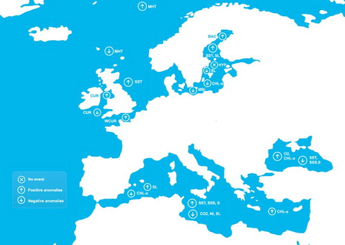
5.2. Anomalous changes during the year 2016

Prevailing conditions of the so-called ‘cold event’ in the subpolar North Atlantic occurred also during the year 2016 (Figure 5.2.1). A concurrent ‘warm event’ is reported in the western subtropical North Atlantic, and a number of Essential and Climate Ocean Variables such as ocean temperature and salinity, ocean heat content, sea level and sea-to-air CO₂ flux undergo these changes simultaneously. Deep convection has been monitored in the central Labrador Sea during winter 2016. In the tropical Atlantic, anomalous high sea surface salinity, currents and sea-to-air CO₂ fluxes are detected, whereas the northward meridional heat transport is anomalously low.

The sea ice extent in the Antarctic decreased dramatically over the last month of the year 2016 and showed the smallest values over the past two decades. This low Antarctic sea ice extent in 2016 is associated with anomalous warm atmospheric surface temperatures, driven by anomalous strong north-westerly winds in the Atlantic and Pacific sectors. In the Arctic, continue dropping in sea ice extent and volume in 2016 (Figure 5.2.1) is related to anomalous high ocean heat transport through Fram and Bering straits into the Arctic region (Figure 5.2.2). In addition, the highest freshwater content in the last 24 years has been observed in the Arctic.

In the subpolar North Pacific, anomalous low values of sea surface temperature, nitrates, sea-to-air CO₂ flux are reported (Figure 5.2.1). In the northern subtropics, a zonal seesaw pattern dominates with high ocean heat content and sea level values in the east, and low values in the west. The tropical Pacific is generally warm at the surface and shows strong currents and low chlorophyll-a concentration. In addition, a zonal seesaw pattern characterises the tropics with positive anomalies of sea surface salinity and negative anomalies of sea level and ocean heat content, which are counteracted in the eastern tropics.

The Indian Ocean shows anomalous high values for sea surface temperature and anomalous low chlorophyll-a values during 2016 (Figure 5.2.1). The northern tropical and subtropical areas are characterised by anomalous high sea level and ocean heat content, and vice-versa in the southern hemisphere. Anomalous low heat and volume transport through the Indonesian Throughflow is reported.

In the Mediterranean Sea, temperature and salinity were anomalously high in almost the entire basin and air-to-sea CO₂ flux and nitrate were anomalously low (Figure 5.2.2). In the eastern and central basin, sea level (thermosteric driven) and chlorophyll-a were anomalously negative and positive in the western basin.

In the Black Sea, observations indicate ongoing deoxygenation with an average oxygen penetration depth of 72 m in 2016, against 90 m in 2010–2015 and 140 m in 1955. Moreover, anomalous strong positive sea surface temperature and salinity anomalies are reported over the entire basin (Figure 5.2.2). A significant negative anomaly in chlorophyll-a concentration can be observed in the whole basin.

No open sea hypoxia events are reported in the Baltic Sea (Figure 5.2.2). A zonal seesaw pattern dominates the Baltic Sea with low sea surface salinity in the east, and high values in the western part. Surface waters of the entire basin are anomalously warm, and absolute sea level is high. An inflow of water from the North Sea into the Baltic Sea through the Danish strait is reported during winter 2016/2017, but is not categorised as Major Baltic Inflows. Chlorophyll-a in the Baltic Sea is higher in the Bothanian Bay and low in Kattegat, Gulf of Riga and Gulf of Finland. The cyanobacteria bloom in 2016 has started in late August and lasted until 21 September, with particular signatures in the eastern and western Gotland Basin. A new record (since 1922) low sea level was observed at the Bothanian Bay station Kemi caused by strong northeasterly winds and weak sea ice conditions.

The North West Shelf area undergoes anomalous positive sea surface temperatures, and low sea surface salinity conditions (Figure 5.2.2). In the annual mean, the surface current magnitudes were weaker in the Celtic Sea, and stronger in the Irish Sea, than in the climatology. In addition, some regions have some of the strongest positive winter anomalies, particularly through the Dover Strait.

At the entrance to the Arctic, evidence exists of a strong increase in the northward heat transport through the Fram Strait (Figure 5.2.2). Upstream in the Færøy-Shetland Channel, however, there is an indication of decreased northward Atlantic Water transport in 2016 that is likely to affect the Nordic Seas and Arctic heat budgets in the years to come due to the advective nature of the Nordic Seas.

References

- CMEMS . 2014. Technical annex to the delegation agreement with Mercator Ocean for the implementation of the Copernicus Marine Environment Monitoring Service (CMEMS). www.copernicus.eu/sites/default/files/library/CMEM_TechnicalAnnex_PUBLIC.docx.pdf .
- CMEMS . 2016. High level service evolution strategy, a document prepared by Mercator Ocean with the support of the CMEMS STAC.
- Hernandez F , Blockley E , Brassington GB , Davidson F , Divakaran P , Drévillon M , Ishizaki S , Garcia-Sotillo M , Hogan PJ , Lagemaa P , et al. 2015. Recent progress in performance evaluations and near real-time assessment of operational ocean products. J Oper Oceanogr. 8(2):s221–s238. doi:10.1080/1755876X.2015.1050282.
- IPCC. 2013. Climate change 2013: The physical science basis. Contribution of working group I to the fifth assessment report of the intergovernmental panel on climate change [Stocker TF, Qin D, Plattner G-K, Tignor M, Allen SK, Boschung J, Nauels A, Xia Y, Bex V, Midgley PM, editors]. Cambridge: Cambridge University Press, 1535. doi:10.1017/CBO9781107415324.
- Le Quéré C , Andrew RM , Canadell JG , Sitch S , Korsbakken JI , Peters GP , Manning AC , Boden TA , Tans PP , Houghton RA , et al. 2016. Global carbon budget 2016. Earth Syst Sci Data. 8(2):605–649. doi: 10.5194/essd-8-605-2016
- Le Traon PY , et al. 2017. The Copernicus marine environmental monitoring service: main scientific achievements and future prospects. Mercator Ocean J. 56. https://www.mercator-ocean.fr/wp-content/uploads/2017/06/Journal56_SpecialV6.pdf .
- OECD . 2016. The ocean economy in 2030. Paris : OECD Publishing. doi:10.1787/9789264251724-en.
- Turpin V , Remy E , Le Traon PY. 2016. How essential are Argo observations to constrain a global ocean data assimilation system? Ocean Sci., 12, 257–274. doi: 10.5194/os-12-257-2016
- UN . 2017. Report of the United Nations conference to support the implementation of sustainable development goal 14: Conserve and sustainably use the oceans, seas and marine resources for sustainable development (Advance unedited version). https://sustainabledevelopment.un.org/content/documents/15662FINAL_15_June_2017_RepoRe_Goal_14.pdf .
- von Schuckmann K , Le Traon PY , Alvarez-Fanjul E , Axell L , Balmaseda M , Breivik LA , Brewin RJW , Bricaud C , Drevillon M , Drillet Y , et al. 2016. The Copernicus Marine Environment Monitoring Service Ocean State report. J Oper Oceanogr. 9:s235–s320. doi:10.1080/1755876X.2016.1273446.
- Armour KC , Marshall J , Scott JR , Donohoe A , Newsom ER. 2016. Southern Ocean warming delayed by circumpolar upwelling and equatorward transport. Nat Geosci. 9(7):549–554. doi: 10.1038/ngeo2731
- Assmy P , Fernández-Méndez M , Duarte P , Meyer A , Randelhoff A , Mundy CJ , Olsen LM , Kauko HM , Bailey A , Chieric M , et al. 2017. Leads in Arctic pack ice enable early phytoplankton blooms below snow-covered sea ice. Scientific Reports, 7, 40850. doi: 10.1038/srep40850
- Beckley BD , Callahan PS , Hancock III, DW , Mitchum GT , Ray RD. 2017. On the “cal mode” correction to TOPEX satellite altimetry and its effect on the global mean sea level time series. J Geophys Res-Oceans. 122:8371–8384. doi:10.1002/2017JC013090
- Boyer T , Domingues CM , Good SA , Johnson GC , Lyman JM , Ishii M , Gourestki V , Willis JK , Antonov J , Wijffels S , et al. 2016. Sensitivity of global upper-ocean heat content estimates to mapping methods, XBT bias corrections, and baseline climatologies. J Clim. 29. doi:10.1175/JCLI-D-15-0801.1.
- Carmack EC , Yamamoto-Kawai M , Haine TWN , Bacon S , Bluhm BA , Lique C , Melling H , Polyakov IV , Straneo F , Timmermans ML , Williams WJ. 2016. Freshwater and its role in the Arctic marine system: sources, disposition, storage, export, and physical and biogeochemical consequences in the Arctic and global oceans. J Geophys Res Biogeosci. 121:675–717. doi: 10.1002/2015JG003140
- Curry R , Dickson B , Yashayaev I. 2003. A change in the freshwater balance of the Atlantic Ocean over the past four decades. Nature. 426:826–829. doi:10.1038/nature02206
- Dai A , Qian T , Trenberth KE. 2009. Changes in continental freshwater discharge from 1948 to 2004. J Clim. 22:2773–2792. doi: 10.1175/2008JCLI2592.1
- Dettinger MD , Diaz HF. 2000. Global characteristics of stream flow seasonality and variability. J Hydrometeor. 1:289–310. doi: 10.1175/1525-7541(2000)001<0289:GCOSFS>2.0.CO;2
- Dieng HB , Cazenave A , Meyssignac B , von Schuckmann K , Palanisamy H. 2017. Sea and land surface temperatures, ocean heat content, Earth’s energy imbalance and net radiative forcing over the recent years. Int J Climatol. 37:218–229. doi:10.1002/joc.4996.
- Durack PJ. 2015. Ocean salinity and the global water cycle. Oceanography. 28(1):20–31. doi: 10.5670/oceanog.2015.03.
- Durack PJ , Lee T , Vinogradova NT , Stammer D. 2016. Keeping the lights on for global ocean salinity observation. Nat Clim Chang. 6:228–231. doi:10.1038/nclimate2946.
- Durack PJ , Wijffels SE , Gleckler PJ. 2014. Long-term sea-level change revisited: the role of salinity. Environ Res Lett 9:114017. doi:10.1088/1748-9326/9/11/114017.
- England MH , McGregor S , Spence JP , Meehl GA , Timmermann A , Cai W , Gupta AS , McPhaden MJ , Purich A , Santoso A. 2014. Recent intensification of wind-driven circulation in the Pacific and the ongoing warming hiatus. Nat Clim Change. 4(3):222–227. doi:10.1038/nclimate2106.
- Forget G , Wunsch C. 2007. Estimated global hydrographic variability. J Phys Oceanogr. 37:1997–2008. doi:10.1175/JPO3072.1.
- Frankignoul C , de Coëtlogon G , Joyce TM , Dong S. 2001. Gulf stream variability and ocean-atmosphere interactions. J Phys Oceanogr. 31:3516–3529. doi: 10.1175/1520-0485(2002)031<3516:GSVAOA>2.0.CO;2
- Han W , Meehl GA , Stammer D , Hu A , Hamlington B , Kenigson J , Palanisamy H , Thompson P. 2017. Spatial patterns of sea level variability associated with natural internal climate modes. Surv Geophys. 38:217–250. doi:10.1007/s10712-016-9386-y.
- Horvat C , Jones DR , Iams S , Schroeder D , Flocco D , Feltham D. 2017. The frequency and extent of sub-ice phytoplankton blooms in the Arctic Ocean. Sci Adv. 3:e1601191. doi: 10.1126/sciadv.1601191
- IFSOO, 2012 . 2012. A framework for ocean observing. By the task team for an integrated framework for sustained ocean observing, UNESCO 2012, IC/INF-1284. doi:10.5270/OceanObs09-FOO.
- IPCC 5th Assessment Report . 2013. The physical Science Basis. Contribution of Working Group I to the Fifth Assessment Report of the Intergouvernmental Panel on Climate Change.
- Kuhlbrodt T , Griesel A , Montoya M , Levermann A , Hofmann M , Rahmstorf S. 2007. On the driving processes of the Atlantic meridional overturning circulation. Rev Geophys. 45(2):RG2001. doi: 10.1029/2004RG000166
- Legeais J-F , von Schuckmann K , Dagneaux Q , Melet A , Meyssignac B , Bonaduce A , Ablain M , Pérez Gomez B. 2016. Sea level. In von Schukmann et al., 2016. The Copernicus Marine Environment Monitoring Service Ocean State Report. J Oper Oceanogr. 9(sup2): s235–s320. doi:10.1080/1755876X.2016.1273446.
- Lenoir S , Beaugrand G , Lecuyer E. 2011. Modelled spatial distribution of marine fish and projected modifications in the North Atlantic Ocean. Global Change Biol. 17(1):115–129. doi:10.1111/j.1365-2486.2010.02229.x.
- Le Quéré C , Andrew RM , Canadell JG , Sitch S , Korsbakken JI , Korsbakken JI , Peters GP , Manning AC , Boden TA , Tans PP , et al. 2016. Global carbon budget 2016. Earth Syst Sci Data. 8(2):605–649. doi: 10.5194/essd-8-605-2016
- Llovel W , Lee T. 2015. Importance and origin of halosteric contribution to sea level change in the southeast Indian Ocean during 2005–2013. Geophys Res Lett. 42(4):1148–1157. doi: 10.1002/2014GL062611
- Lüthi D , Le Floch M , Bereiter B , Blunier T , Barnola JM , Siegenthaler U , Raynaud D , Jouzel J , Fischer H , Kawamura K , et al. 2008. High-resolution carbon dioxide concentration record 650,000–800,000 years before present. Nature. 453(7193):379–382. doi: 10.1038/nature06949
- O’Kane TJ , Monselesan DP , Maes C. 2016. On the stability and spatiotemporal variance distribution of salinity in the upper ocean. J Geophys Res Oceans. 121(6):4128–4148. doi: 10.1002/2015JC011523
- Penduff T , Juza M , Barnier B , Zika J , Dewar WK , Treguier AM , Molines JM , Audiffren N. 2011. Sea level expression of intrinsic and forced ocean variabilities at interannual time scales. J Clim. 24(21):5652–5670. doi: 10.1175/JCLI-D-11-00077.1
- Riser SC , Freeland HJ , Roemmich D , Wijffels S , Troisi A , Belbéoch M , Gilbert D , Xu J , Pouliquen S , Thresher A , et al. 2016. Fifteen years of ocean observations with the global Argo array. Nat Clim Chang. 6(2):145–153. doi: 10.1038/nclimate2872
- Robinson IS. 2004. Measuring the oceans from space: the principles and methods of satellite oceanography. Chichester : Springer Praxis Books.
- Roemmich D , Church J , Gilson J , Monselesan D , Sutton P , Wijffels S. 2015. Unabated planetary warming and its ocean structure since 2006. Nat Clim Chang. 5:240–245. doi:10.1038/NCLIMATE2513.
- Sarmiento JL , Gruber N. 2006. Ocean biogeochemical dynamics. Princeton : Princeton University Press.
- Sérazin G , Penduff T , Grégorio S , Barnier B , Molines JM , Terray L. 2015. Intrinsic variability of sea level from global ocean simulations: spatiotemporal scales. J Clim. 28(10):4279–4292. doi: 10.1175/JCLI-D-14-00554.1
- Sprintall J , Gordon AL , Koch-Larrouy A , Lee T , Potemra JT , Kandaga Pujiana K , Wijffels SE. 2014. The Indonesian seas and their role in the coupled ocean–climate system. Nat Geosci. 7:487–492. doi:10.1038/ngeo2188.
- Trenberth KE , Fasullo JT , Mackaro J. 2011. Atmospheric moisture transports from ocean to land and global energy flows in reanalyses. J Clim. 24:4907–4924. doi:10.1175/2011JCLI4171.1.
- Vargas-Hernandez JM , Wijffels S , Meyers G , Holbrook NJ. 2015. Slow westward movement of salinity anomalies across the tropical South Indian Ocean. J Geophys Res Oceans. 120(8):5436–5456. doi: 10.1002/2015JC010933
- Ward PJ , Beets W , Bouwer LM , Aerts CJCH , Renssen H. 2010. Sensitivity of river discharge to ENSO. Geophys Res Lett. 37(12):L12402. doi: 10.1029/2010GL043215
- Ward PJ , Eisner S , Flörke M , Dettinger MD , Kummu M. 2014a. Annual flood sensitivities to El Niño–Southern Oscillation at the global scale. Hydrol Earth Syst Sci. 18:47–66. doi: 10.5194/hess-18-47-2014
- Ward PJ , Jongman B , Kummu M , Dettinger MD , Weiland FCS , Winsemius HC. 2014b. Strong influence of El Niño Southern Oscillation onflood risk around the world Proc. Natl Acad Sci., USA. 111:5659–5664.
- Yang H , Liu J , Lohmann G , Shi X , Hu Y , Chen X. 2016. Ocean-atmosphere dynamics changes associated with prominent ocean surface turbulent heat fluxes trends during 1958–2013. Ocean Dynam. 66:353–365. doi:10.1007/s10236-016-0925-3.
- Yu L , Jin X , Josey SA , Lee T , Kumar A , Wen C , Xue Y. 2017. The global ocean water cycle in atmospheric reanalysis, satellite, and ocean salinity. J Clim. 30(10):3829–3852. doi:10.1175/JCLI-D-16-0479.1.
Section 1.1
- Abraham JP , Baringer M , Bindoff NL , Boyer T , Cheng LJ , Church JA , Conroy JL , Domingues CM , Fasullo JT , Gilson J , et al. 2013. Monitoring systems of global ocean heat content and the implications for climate change, a review. Rev Geophys. 51:450–483. doi:10.1002/rog.20022.
- Buongiorno Nardelli B , Tronconi C , Pisano A , Santoleri R. 2013. High and ultra-high resolution processing of satellite Sea surface temperature data over Southern European Seas in the framework of MyOcean project. Remote Sens Environ. 129:1–16. doi:10.1016/j.rse.2012.10.012.
- Donlon CJ , Martin M , Stark J , Roberts-Jones J , Fiedler E , Wimmer W. 2012. The operational sea surface temperature and sea ice analysis (OSTIA) system. Remote Sens Environ. 116:140–158. ISSN 0034-4257. doi:10.1016/j.rse.2010.10.017.
- Droghei R , Buongiorno Nardelli B , Santoleri R. 2016. Combining in-situ and satellite observations to retrieve salinity and density at the ocean surface. J Atmos Ocean Technol. 33:1211–1223. doi:10.1175/JTECH-D-15-0194.1.
- Droghei R , Buongiorno Nardelli B , Santoleri R. 2018. A new global sea surface salinity and density dataset from multivariate observations (1993–2016). Front Mar Sci. 5(March):1–13. doi:10.3389/fmars.2018.00084.
- Escudier P , Couhert A , Mercier F , Mallet A , Thibaut P , Tran N , Amarouche L , Picard B , Carrère L , Dibarboure G , et al. 2017. Satellite radar altimetry: principle, geophysical correction and orbit, accuracy and precision. In: Stammer D, Cazenave A, guest editors. CRC Book on satellite altimetry.
- Kennedy J , Dunn R , McCarthy M , Titchner H , Morice C. 2017. Global and regional climate in 2016. Weather. 72:219–225. doi:10.1002/wea.3042.
- Liang Y , Chou C , Yu J , Lo M. 2016. Mapping the locations of asymmetric and symmetric discharge responses in global rivers to the two types of El Niño. Environ Res Lett. 11(4). doi:10.1088/1748-9326/11/4/044012.
- Milliman JD , Farnsworth KL , Jones PD , Xu KH , Smith LC. 2008. Climatic and anthropogenic factors affecting river discharge to the global ocean, 1951–2000. Global Planet Chang. 62(3–4):187–194. doi: 10.1016/j.gloplacha.2008.03.001
- Paek H , Yu JY , Qian C. 2017. Why were the 2015/2016 and 1997/1998 extreme El Niño different? Geophys Res Lett. 44:1848–1856.
- Pezzulli S , Stephenson DB , Hannachi A. 2005. The variability of seasonality. J Clim. 18:71–88. doi:10.1175/JCLI-3256.1.
- Roquet H , Pisano A , Embury O. 2016. Sea surface temperature. In: von Schuckmann et al. 2016, The Copernicus marine environment monitoring service ocean state report. J Oper Ocean. 9(suppl. 2). doi:10.1080/1755876X.2016.1273446.
- Sen PK. 1968. Estimates of the regression coefficient based on Kendall’s tau. J Am Statist Assoc. 63:1379–1389. doi: 10.1080/01621459.1968.10480934
- Shapiro GI , Aleynik DL , Mee LD. 2010. Long term trends in the sea surface temperature of the Black Sea. Ocean Sci. 6:491–501. doi:10.5194/os-6-491-2010.
Section 1.2
- Ablain M , Cazenave A , Larnicol G , Balmaseda M , Cipollini P , Faugère Y , Fernandes MJ , Henry O , Johannessen JA , Knudsen P , et al. 2015. Improved sea level record over the satellite altimetry era (1993–2010) from the climate change initiative project. Ocean Sci. 11:67–82. doi:10.5194/os-11-67-2015.
- Ablain M , Larnicol G , Faugere Y , Cazenave A , Meyssignac B , Picot N , Benveniste J. 2012. Error characterization of altimetry measurements at climate scales. Proceedings of the ‘20 Years of Progress in Radar Altimetry’ symposium; Venice, Italy; September 24–29. In: Benveniste J, Morrow R, editors, ESA Special Publication SP-710. doi:10.5270/esa.sp-710.altimetry2012.
- Ablain M , Legeais JF , Prandi P , Fenoglio-Marc L , Marcos M , Dieng HB , Benveniste J , Cazenave A. 2017. Satellite altimetry-based Sea level at global and regional scales. Surv Geophys. 38:7–31. doi:10.1007/s10712-016-9389-8.
- Chambers DP , Cazenave A , Champollion N , Dieng H , Llovel W , Forsberg R , von Schuckmann K , Wada Y. 2017. Evaluation of the global mean sea level budget between 1993 and 2014. Surv Geophys. 38:309–327. doi:10.1007/978-3-319-56490-6_14
- Chen X , Zhang X , Church JA , Watson CS , King MA , Monselesan D , Legresy B , Harig C. 2017. The increasing rate of global mean sea-level rise during 1993–2014. Nature Clim Change. 7:492–495. doi:10.1038/nclimate3325.
- Cipollini P , Birol F , Fernandes MJ , Obligis E , Passaro M , Strub PT , Valladeau G , Vignudelli S , Wilkin J. 2017b. Satellite altimetry in coastal regions. In: Stammer D, Cazenave A, guest editors. CRC Book on satellite altimetry.
- Cipollini P , Calafat FM , Jevrejeva S , Melet A , Prandi P. 2017a. Monitoring sea level in the coastal zone with satellite altimetry and tide gauges. Sur Geophys. 38:35–59. doi:10.1007/978-3-319-56490-6_3.
- Couhert A , Cerri L , Legeais JF , Ablain M , Zelensky N , Haines B , Lemoine F , Bertiger W , Desai S , Otten M. 2014. Towards the 1mm/y stability of the radial orbit error at regional scales. Adv Space Res. 55:2–23. doi:10.1016/j.asr.2014.06.041.
- Durack PJ , Wijffels SE. 2010. Fifty-year trends in global ocean salinities and their relationship to broad-scale warming. J Clim. 23:4342–4362. doi:10.1175/2010JCLI3377.1.
- Fukumori I , Menemenlis D , Lee T. 2007. A near-uniform basin-wide sea level fluctuation of the Mediterranean Sea. J Phys Ocean. 37:338–358. doi: 10.1175/JPO3016.1
- Legeais J-F , Ablain M , Thao S. 2014. Evaluation of wet troposphere path delays from atmospheric reanalyses and radiometers and their impact on the altimeter sea level. Ocean Sci. 10:893–905. doi:10.5194/os-10-893-2014.
- Legeais J-F , Ablain M , Zawadzki L , Zuo H , Johannessen JA , Scharffenberg MG , Fenoglio-Marc L , Fernandes MJ , Andersen O , Rudenko S , et al. 2017. An accurate and homogeneous altimeter sea level record from the ESA climate change initiative. Earth Syst Sci Data Discuss. doi:10.5194/essd-2017-116, in review.
- Legeais J-F , Ablain M , Zawadzki L , Zuo H , Johannessen JA , Scharffenberg MG , Fenoglio-Marc L , Fernandes MJ , Andersen OB , Rudenko S , et al. 2018. An improved and homogeneous altimeter sea level record from the ESA Climate Change Initiative. Earth Syst Sci Data. 10:281–301. doi:10.5194/essd-10-281-2018.
- MacIntosh CR , Merchant CJ , von Schuckmann K. 2017. Uncertainties in steric sea level change estimation during the satellite altimeter era: concepts and practices. Surv Geophys. 38:61–89. doi:10.1007/978-3-319-56490-6_4
- Melet A , Almar R , Meyssignac B. 2016. What dominates sea level at the coast: a case study for the Gulf of Guinea. Ocean Dynam. 66:623–636. doi:10.1007/s10236-016-0942-2.
- Meyssignac B , Piecuch CG , Merchant CJ , Racault M-F , Palanisamy H , MacIntosh C , Sathyendranath S , Brewin R. 2017. Causes of the regional variability in observed Sea level, Sea surface temperature and ocean colour over the period 1993–2011. Surv Geophys. 38:191–219. doi:10.1007/978-3-319-56490-6_9
- Meyssignac B , Salas-Melia D , Becker M , Llovel W , Cazenave A. 2012. Tropical pacific spatial trend patterns in observed sea level: internal variability and/or anthropogenic signature? Clim Past. 8:787–802. doi:10.5194/cp-8-787-2012.
- Mohrholz V , Naumann MM , Nausch G , Krüger S , Gräwe U. 2015. Fresh oxygen for the Baltic Sea – an exceptional saline inflow after a decade of stagnation. J Mar Sys. 148:152–166. doi: 10.1016/j.jmarsys.2015.03.005
- Nerem RS , Ablain M , Cazenave A , Church J , Leuliette E. 2017. A 25-year long satellite altimetry-based global mean sea level record: Closure of the sea level budget & missing components. In: Stammer D, Cazenave A, guest editors. CRC Book on satellite altimetry.
- Palanisamy H , Meyssignac B , Cazenave A , Delcroix T. 2015. Is anthropogenic sea level fingerprint already detectable in the Pacific Ocean? Environ Res Lett. 10(2015):084024. doi:10.1088/1748-9326/10/8/084024.
- Pisano A , Buongiorno Nardellia B , Tronconia C , Santoleria R. 2016. The new Mediterranean optimally interpolated pathfinder AVHRR SST dataset (1982–2012). Remote Sens Environ. 176:107–116. doi:10.1016/j.rse.2016.01.019.
- Peltier R. 2004. Global glacial isostasy and the surface of the ice-age earth: the ICE-5G (VM2) model and GRACE. Annu Rev Earth Planet Sci. 32:111–149. doi: 10.1146/annurev.earth.32.082503.144359
- Pinardi N , Masetti E. 2000. Variability of the large scale general circulation of the Mediterranean Sea from observations and modelling: a review. Palaeogeogr Palaeocl. 158:153–173. doi:10.1016/S0031-0182(00)00048-1.
- Pujol M-I , Faugère Y , Taburet G , Dupuy S , Pelloquin C , Ablain M , Picot N. 2016. DUACS DT2014: the new multi-mission altimeter data set reprocessed over 20 years. Ocean Sci. 12:1067–1090. doi:10.5194/os-12-1067-2016.
- Roberts-Jones J , Fiedler EK , Martin MJ. 2012. Daily, global, high-resolution SST and Sea Ice reanalysis for 1985–2007 using the OSTIA system. J Clim. 25:6215–6232. doi:10.1175/JCLI-D-11-00648.1.
- Schiermeier Q. 2015. Hunting the Gozilla El Nino. Nature. 526:490–491. doi:10.1038/526490a.
- Spada G. 2017. Glacial isostatic adjustment and contemporary sea level rise: an overview. Surv Geophys. 38:155–187. doi: 10.1007/978-3-319-56490-6_8
- Stammer D , Cazenave A , Ponte RM , Tamisiea ME. 2013. Causes for contemporary regional sea level changes. Annu Rev Mar Sci. 5:21–46. doi:10.1146/annurev-marine-121211-172406.
- Tamisiea ME , Mitrovica JX. 2011. The moving boundaries of sea level change: understanding the origins of geographic variability. Oceanography. 24(2):24–39. doi: 10.5670/oceanog.2011.25
- Watson CS , White NJ , Church JA , King MA , Burgette RJ , Legresy B. 2015. Unabated global mean sea-level rise over the satellite altimeter era. Nat Clim Chang. 5:565–568. doi:10.1038/NCLIMATE2635.
- Zawadzki L , Ablain M. 2016. Accuracy of the mean sea level continuous record with future altimetric missions: jason-3 vs. sentinel-3a. Ocean Sci. 12:9–18. doi:10.5194/os-12-9-2016.
Section 1.3
- Drévillon M , Balmaseda M , Gasparin F , von Schuckmann K , Greiner E. 2016. The 2015 El Niño event, in von Schuckmann et al., the Copernicus Marine Environment Monitoring Service Ocean State report. J Oper Oceanogr. 9. doi:10.1080/1755876X.2016.1273446.
- Schott FA , JP McCreary Jr . 2001. The monsoon circulation of the Indian Ocean. Prog Oceanogr. 51:1–123. doi: 10.1016/S0079-6611(01)00083-0
- Tinker J , O’Dea E , Sykes P , Hyder P , Holt J , Dye S. 2016. Regional seas: north-west European shelf seas, in von schuckmann et al., the Copernicus marine environment monitoring service ocean state report. J Oper Oceanogr. 9. doi:10.1080/1755876X.2016.1273446.
Section 1.4
- Chevallier M , Smith GC , Dupont F , Lemieux J-F , Forget G , Fujii Y , Hernandez F , Msadek R , Peterson KA , Storto A , et al. 2016. Intercomparison of the Arctic sea ice cover in global ocean–sea ice reanalyses from the ORA-IP project. Clim Dyn. 49:1107–1136. doi: 10.1007/s00382-016-2985-y
- Ivanova N , Johannessen OM , Pedersen LT , Tonboe RT. 2014. Retrieval of Arctic Sea ice parameters by satellite passive microwave sensors: A comparison of eleven sea ice concentration algorithms. IEEE Trans Geosci Remote Sens. 52:7233–7246. doi: 10.1109/TGRS.2014.2310136
- Kauker F , Kaminski T , Ricker R , Toudal-Pedersen L , Dybkjaer G , Melsheimer C , Eastwood S , Sumata H , Karcher M , Gerdes R. 2015. Seasonal sea ice predictions for the Arctic based on assimilation of remotely sensed observations. Cryosph Discuss. 9:5521–5554. doi: 10.5194/tcd-9-5521-2015
- Ricker R , Hendricks S , Helm V , Skourup H , Davidson M. 2014. Sensitivity of CryoSat-2 Arctic sea-ice freeboard and thickness on radar-waveform interpretation. Cryosphere. 8:1607–1622. doi: 10.5194/tc-8-1607-2014
- Samuelsen A , Breivik L-A , Raj RP , Garric G , Axell L , Olason E. 2016. 1.7 Sea ice. In: Copernicus Mar Environ Monit Serv Ocean State Report, von Schuckmann et al. [place unknown]; p. 88.
- Tian-Kunze X , Kaleschke L , Maaß N , Mäkynen M , Serra N , Drusch M , Krumpen T. 2014. SMOS-derived thin sea ice thickness: algorithm baseline, product specifications and initial verification. Cryosphere. 8:997–1018. doi: 10.5194/tc-8-997-2014
- Uiboupin R , Axell L , Raudsepp U , Sipelgas L. 2010. Comparison of operational ice charts with satellite based ice concentration products in the Baltic Sea. 2010 IEEE/OES US/EU Balt Int Symp Balt 2010.
- Xie J , Counillon F , Bertino L , Tian-Kunze X , Kaleschke L. 2016. Benefits of assimilating thin sea ice thickness from SMOS into the TOPAZ system. Cryosphere. 10:2745–2761. doi: 10.5194/tc-10-2745-2016
- Zygmuntowska M , Rampal P , Ivanova N , Smedsrud LH. 2014. Uncertainties in Arctic sea ice thickness and volume: New estimates and implications for trends. Cryosphere. 8:705–720. doi: 10.5194/tc-8-705-2014
Section 1.5
- Jackson T , Sathyendranath S , Mélin F. 2017. An improved optical classification scheme for the ocean colour essential climate variable and its applications. Remote Sens Environ. doi:10.1016/j.rse.2017.03.036.
- Longhurst AR. 2006. Ecological geography of the sea. 2nd ed. San Diego (CA) : Academic Press.
- Müller D , Krasemann H , Brewin RJW , Brockmann C , Deschamps P-Y , Doerffer R , Fomferra N , Franz BA , Grant MG , Groom SB , et al. 2015. The ocean colour climate change initiative: I. A methodology for assessing atmospheric correction processors based on in-situ measurements. Remote Sens Environ. 162:242–256. doi: 10.1016/j.rse.2013.11.026
- Sathyendranath S , Brewin RJW , Jackson T , Mélin F , Platt T. 2017. Ocean-colour products for climate-change studies: what are their ideal characteristics? Remote Sens Environ. 203:125–138. doi:10.1016/j.rse.2017.04.017.
- Sathyendranath S , Grant M , Brewin RJW , Brockmann C , Brotas V , Chuprin A , Doerffer R , Dowell M , Farman A , Groom S , et al. , 2018. ESA Ocean Colour Climate Change Initiative (Ocean_Colour_cci): Version 3.1 Data. Centre for Environmental Data Analysis. http://catalogue.ceda.ac.uk/uuid/9c334fbe6d424a708cf3c4cf0c6a53f5
- Vantrepotte V , Mélin F. 2009. Temporal variability of 10-year global Sea WiFS time-series of phytoplankton chlorophyll a concentration. ICES J Mar Sci. 66:1547–1556. doi:10.1093/icesjms/fsp107.
Section 1.6
- Radenac MH , Menkès C , Vialard J , Moulin C , Dandonneau Y , Delcroix T , Dupouy C , Stoens A , Deschamps PY. 2001. Modeled and observed impacts of the 1997–1998 El Niño on nitrate and new production in the equatorial Pacific. J Geophys Res Ocean. 106(C11):26879–26898. doi: 10.1029/2000JC000546
- Wang X , Christian JR , Murtugudde R , Busalacchi AJ. 2005. Ecosystem dynamics and export production in the central and eastern equatorial Pacific: a modeling study of impact of ENSO. Geophys Res Lett. 32(2):LO2608. doi: 10.1029/2004GL021538
Section 1.7
- Bakker DCE , Pfeil B , Smith K , Hankin S , Olsen A , Alin SR , Cosca C , Harasawa S , Kozyr A , Nojiri Y , et al. 2014. An update to the surface ocean CO2 atlas (SOCAT version 2). Earth Syst Sci Data. 6:69–90. doi: 10.5194/essd-6-69-2014
- Ballantyne AP , Alden CB , Miller JB , Tans PP , White JWC. 2012. Increase in observed net carbon dioxide uptake by land and oceans during the past 50 years. Nature. 488(7409):70–72. doi: 10.1038/nature11299
- Bauer JE , Cai WJ , Raymond PA , Bianchi TS , Hopkinson CS , Regnier PA. 2013. The changing carbon cycle of the coastal ocean. Nature. 504(7478):61–70. doi: 10.1038/nature12857
- Bopp L , Resplandy L , Orr JC , Doney SC , Dunne JP , Gehlen M , Halloran P. , Heinze C. , Ilyina T. , Séférian R. , et al. 2013. Multiple stressors of ocean ecosystems in the twenty-first century: projections with CMIP5 models. Biogeosciences. 10:6225–6245. doi: 10.5194/bg-10-6225-2013
- Bourgeois T , Orr JC , Resplandy L , Terhaar J , Ethé C , Gehlen M , Bopp L. 2016. Coastal-ocean uptake of anthropogenic carbon. Biogeosciences. 13(14):4167–4185. doi: 10.5194/bg-13-4167-2016
- Ciais P , Sabine C , Bala G , Bopp L , Brovkin V , Canadell J , Chhabra A , DeFries R , Galloway J , Heimann , et al. 2013. Carbon and other biogeochemical cycles. In climate change 2013: The physical science basis. Contribution of Working Group I to the Fifth Assessment Report of the Intergovernmental Panel on Climate Change. Chapter 6.
- Conway TJ , Tans PP , Waterman LS , Thoning KW , Kitzis DR , Masarie KA , Zhang N. 1994. Evidence for interannual variability of the carbon cycle from the NOAA/CMDL global air sampling network. J Geophys Res. 99(22):831–22.
- Cossarini G , Lazzari P , Solidoro C. 2015. Spatiotemporal variability of alkalinity in the Mediterranean Sea. Biogeosciences. 12(6):1647–1658. doi: 10.5194/bg-12-1647-2015
- DeVries T , Holzer M , Primeau F. 2017. Recent increase in oceanic carbon uptake driven by weaker upper-ocean overturning. Nature. 542:215–218. doi:10.1038/nature21068.
- Gehlen M , Gruber N , Gangstø R , Bopp L , Oschlies A. 2011. Biogeochemical consequences of ocean acidification and feedbacks to the earth system. Ocean Acidif. 1:230–248.
- Jacobson AR , Mikaloff Fletcher SE , Gruber N , Sarmiento JL , Gloor M. 2007. A joint atmosphere-ocean inversion for surface fluxes of carbon dioxide: 1. methods and global-scale fluxes. Global Biogeoche Cycles. 21(1). doi:10.1029/2005GB002556.
- Landschützer P , Gruber N , Bakker DCE , Schuster U. 2014. Recent variability of the global ocean carbon sink. Global Biogeochem Cycle. 28(9):927–949. doi: 10.1002/2014GB004853
- Le Quéré C , Andrew RM , Friedlingstein P , Sitch S , Pongratz J , Manning AC , Korsbakken JI , Zhu D. 2017. Global Carbon Budget 2017. Earth Syst Sci Data. doi:10.5194/essd-2017-123, in review.
- Masarie KA , Tans PP. 1995. Extension and integration of atmospheric carbon dioxide data into a globally consistent measurement record. J Geophys Res. 100(D6):11593–11610. doi: 10.1029/95JD00859
- Melaku Canu D , Ghermandi A , Nunes PALD , Cossarini C , Lazzari P , Solidoro S. 2015. Estimating the value of carbon sequestration ecosystem services in the Mediterranean Sea: an ecological economics approach. Global Environ Change. 32:87–95. doi: 10.1016/j.gloenvcha.2015.02.008
- Resplandy L , Séférian R , Bopp L. 2015. Natural variability of CO2 and O2 fluxes: what can we learn from centuries-long climate models simulations? J Geophys Res Ocean. 120(1):384–404. doi: 10.1002/2014JC010463
- Rödenbeck C , Bakker DC , Gruber N , Iida Y , Jacobson AR , Jones S , Landschützer P , Metzl N , Nakaoka S , Olsen A , et al. 2015. Data-based estimates of the ocean carbon sink variability–first results of the surface ocean pCO2 mapping intercomparison (SOCOM). Biogeosciences. 12:7251–7278. doi: 10.5194/bg-12-7251-2015
- Roy T , Bopp L , Gehlen M , Schneider B , Cadule P , Frölicher TL , Segschneider J , Tjiputra J , Heinze C , Joos F. 2011. Regional impacts of climate change and atmospheric CO2 on future ocean carbon uptake: a multimodel linear feedback analysis. J Clim. 24(9):2300–2318. doi: 10.1175/2010JCLI3787.1
- Sarmiento JL , Gruber N. 2006. Ocean biogeochemical dynamics. Princeton, NJ : Princeton University Press.
- Schott FA , McCreary JP , Johnson GC. 2004. Shallow overturning circulations of the tropical-subtropical oceans. Earth Clim. 147:261–304. doi:10.1029/147GM15.
- Séférian R , Iudicone D , Bopp L , Roy T , Madec G. 2012. Water mass analysis of effect of climate change on air–sea CO2 fluxes: the Southern Ocean. J Clim. 25(11):3894–3908. doi: 10.1175/JCLI-D-11-00291.1
- Séférian R , Ribes A , Bopp L. 2014. Detecting the anthropogenic influences on recent changes in ocean carbon uptake. Geophys Res Lett. 41(16):5968–5977. doi: 10.1002/2014GL061223
- Takahashi T , Sutherland SC , Sweeney C , Poisson A , Metzl N , Tilbrook B , Bates N , Wanninkhof R , Feely RA , Sabine C , et al. 2002. Global sea–air CO2 flux based on climatological surface ocean p CO2, and seasonal biological and temperature effects. Deep Sea Res II: Topical Stud Oceanogr. 49(9):1601–1622. doi: 10.1016/S0967-0645(02)00003-6
- Wanninkhof R. 1992. Relationship between wind speed and gas exchange over the ocean. J Geophys Res Ocean. 97(C5):7373–7382. doi: 10.1029/92JC00188
- World Data Centre for Greenhouse Gases . 2017. [Url visited on June 2017]. http://ds.data.jma.go.jp/gmd/wdcgg/cgi-bin/wdcgg/map_search.cgi .
Section 1.8
- Belmonte Rivas M , Stoffelen A , Verspeek J , Verhoef A , Neyt X , Anderson C. 2017. Cone metrics: a new tool for the intercomparison of scatterometer records. IEEE J Select Topic Appl Earth Obs Remote Sens. 10(5). doi:10.1109/JSTARS.2017.2647842.
- Chelton DB , Schlax MG , Freilich MH , Milliff RF. 2004. Satellite measurements reveal persistent small-scale features in ocean winds. Science. 303(5660):978–983. doi:10.1126/science.1091901.
- Dee DP , Uppala SM , Simmons AJ , Berrisford P , Poli P , Kobayashi S , Andrae U , Balmaseda MA , Balsamo G , Bauer P , et al. 2011. The ERA-interim reanalysis: configuration and performance of the data assimilation system. Q J R Meteorol Soc. 137:553–597. doi:10.1002/qj.828.
- Sandu I , Beljaars A , Bechtold P , Mauritsen T , Balsamo G. 2013. Why is it so difficult to represent stably stratified conditions in numerical weather prediction (NWP) models? J Adv Model Earth Syst. 5:117–133. doi: 10.1002/jame.20013
- Stoffelen A , Aaboe S , Calvet J-C , Cotton J , De Chiara G , Figa Saldaña J , Mouche A , Portabella M , Scipal K , Wagner W. 2017b. Scientific developments and the EPS-SG scatterometer. IEEE J Select Topic Appl Earth Obs Remote Sens. 10(5). doi:10.1109/JSTARS.2017.2696424.
- Stoffelen A , Verspeek J , Vogelzang J , Verhoef A. 2017a. The CMOD7 geophysical model function for ASCAT and ERS wind retrievals. IEEE J Select Topic Appl Earth Obs Remote Sens. 10(5). doi:10.1109/JSTARS.2017.2681806.
- Verhoef A , Vogelzang J , Verspeek J , Stoffelen A. 2017a. Long-term scatterometer wind climate data records. IEEE J Select Topic Appl Earth Obs Remote Sens. 10(5): 2186–2194. doi:10.1109/JSTARS.2016.2615873.
- Verhoef A , Vogelzang J , Stoffelen A. 2017b. ERS L2 winds data record validation report 25 km wind products (OSI-152). Version 1.1. doi:10.15770/EUM_SAF_OSI_0009.
- Vogelzang J , Stoffelen A , Verhoef A , Figa-Saldana J. 2011. On the quality of high-resolution scatterometer winds. J Geophys Res. 116:C10033. doi:10.1029/2010JC006640.
- Wang Z , Stoffelen A , Zhao C , Vogelzang J , Verhoef A , Verspeek J , Lin M , Chen G. 2017. An SST-dependent Ku-band geophysical model function for RapidScat. J Geophys Res-Oceans. 122. doi:10.1002/2016JC012619.
- Wentz FJ , Ricciardulli L , Rodriguez E , Stiles BW , Bourassa MA , Long DG , Hoffman RN , Stoffelen A , Verhoef A , O'Neill LW , et al. 2017. Evaluating and extending the ocean wind climate data record. IEEE J Sel Top Appl. doi:10.1109/JSTARS.2016.2643641.
- Dee DP. 2011. The ERA-Interim reanalysis: configuration and performance of the data assimilation system. Royal Meterol Soc. 137:553–597. doi:10.1002/qj.828.
- Dieng HB , Cazenave A , Meyssignac B , von Schuckmann K , Palanisamy H. 2017. Sea and land surface temperatures, ocean heat content, earth’s energy imbalance and net radiative forcing over the recent years. Int J Climatol. doi:10.1002/joc.4996.
- Doney SC , Ruckelshaus M , Emmett Duffy J , Barry JP , Chan F , English CA , Galindo HM , Grebmeier JM , Hollowed AB , Knowlton N , et al. 2012. Climate change impacts on marine ecosystems. Ann Rev Mar Sci. 4:11–37.
- Drijfhout S , van Oldenborgh GJ , Cimatoribus A. 2012. Is a decline of AMOC causing the warming hole above the North Atlantic in observed and modeled warming patterns? J Clim. 25(24):8373–8379.
- Duchez A , Eleanor F-W , Josey SA , Evans DG , Grist JP , Marsh R , McCarthy GD , Sinha B , Berry DI , Hirschi JJ-M. 2016. Drivers of exceptionally cold North Atlantic Ocean temperatures and their link to the 2015 European heat wave. Environ Res Lett. 11(7):074004. doi:10.1088/1748-9326/11/7/074004.
- Grist JP , Josey SA , Jacobs ZL , Marsh R , Sinha B , van Sebille E. 2016. Extreme air–sea interaction over the North Atlantic subpolar gyre during the winter of 2013–2014 and its sub-surface legacy. Clim Dyn. 46:4027–4045. doi:10.1007/s00382-015-2819-3.
- Hansen J , Sato M , Kharecha P , von Schuckmann K. 2011. Earth’s energy imbalance and implications. Atmos Chem Phys. 11:13421–13449. www.atmos-chem-phys.net/11/13421/2011/ . doi:10.5194/acp-11-13421-2011.
- Kessler WS , McPhaden MJ , Weickmann KM. 1995. Forcing of intraseasonal Kelvin waves in the equatorial Pacific. J Geophys Res: Oceans. 100(C6):10613–10631.
- Marshall J. 2001. North Atlantic climate variability: phenomena, impacts and mechanisms. Int J Climatol. 21:1863–1898.
- Polyakov IV , Pnyushkov AV , Alkire MB , Ashik IM , Baumann TM , Carmack EC , Goszczko I , Guthrie J , Ivanov VV , Kanzow T , et al. 2017. Greater role for Atlantic inflows on sea-ice loss in the Eurasian Basin of the Arctic Ocean. Science. 356(6335):285–291. doi:10.1126/science.aai8204.
- Woollings T , Gregory JM , Pinto JG , Reyers M , Brayshaw DJ. 2012. Response of the North Atlantic storm track to climate change shaped by ocean–atmosphere coupling. Nat Geosci. 5(5):313–317.
- Section 2.1
- Balmaseda MA , Trenberth KE , Källén E. 2013. Distinctive climate signals in reanalysis of global ocean heat content. Geophys Res Lett. 40. doi:10.1002/grl.50382.
- Buckley M , Marshall J. 2016. Observations, inferences, and mechanisms of the Atlantic Meridional Overturning Circulation: a review. Rev Geophys. 54. doi:10.1002/2015RG000493.
- Cazenave A , Dieng H-B , Meyssignac B , von Schuckmann K , Decharme B , Berthier E. 2014. The rate of sea level rise. Nature Geosci. doi:10.1038/NCLIMATE2159.
- Fratianni C , Simoncelli S , Pinardi N , Cherchi A , Grandi A , Dobricic S. 2015. Mediterranean RR 1955–2015 (Version 1) [dataset]. Copernicus Monitoring Environment Marine Service (CMEMS).
- Hansen J , Kharecha P , Sato M , Masson-Delmotte V , Ackerman F , Beerling D , Hearty PJ , Hoegh-Guldberg O , Hsu S-L , Parmesan C , et al. 2013. Scientific prescription to avoid dangerous climate change to protect young people. Future generations, and nature. Plos One. 8:e81648. doi:10.1371/journal.pone.0081648.
- Hansen J , Sato M , Kharecha P , von Schuckmann K. 2011. Earth’s energy imbalance and implications. Atmos Chem Phys 11:13421–13449. www.atmos-chem-phys.net/11/13421/2011/ . doi:10.5194/acp-11-13421-2011.
- IPCC 5th Assessment Report . 2013. The physical science basis. Contribution of Working Group I to the Fifth Assessment Report of the Intergouvernmental Panel on Climate Change.
- Levitus S , Antonov JI , Boyer TP , Baranova OK , Garcia HE , Locarnini RA , Mishonov AV , Reagan JR , Seidov D , Yarosh ES , Zweng MM , et al. 2012. World ocean heat content and thermosteric sealevel change (0–2000 m), 1955–2010. Geophys Res Lett 39:L10603. doi:10.1029/2012GL051106.
- Loeb GN , Lyman JM , Johnson GC , Allan RP , Doelling DR , Wong T , Soden BJ , Stephens GL. 2012. Observed changes in top-of-the-atmosphere radiation and upper-ocean heating consistent within uncertainty. Nat Geosci. 5:110–113.
- Loeb NG , Wielicki BA , Doelling DR , Smith GL , Keyes DF , Kato S , Manalo-Smith N , Wong T. 2009. Toward optimal closure of the earth’s top-of-atmosphere radiation budget. J Clim. 22(3):748–766.
- Mayer M , Haimberger L , Balmaseda MA. 2014. On the energy exchange between tropical ocean basins related to ENSO. J Clim. 27(17):6393–6403.
- Mayer M , Haimberger L , Pietschnig M , Storto A. 2016. Facets of Arctic energy accumulation based on observations and reanalyses 2000–2015. Geophys Res Lett. 43(19):10420–10429. doi:10.1002/2016GL070557.
- Purkey SG , Johnson GC. 2010. Warming of global abyssal and deep southern ocean waters between the 1990s and 2000s: contributions to global heat and sea level rise budgets. J Clim. 23. doi:10.1175/2010JCLI3682.1.
- Riser SC , Freeland HJ , Roemmich D , Wijffels S , Troisi A , Belbéoch M , Gilbert D , Xu J , Pouliquen S , Thresher A , et al. 2016. Fifteen years of ocean observations with the global Argo array. Nat Clim Change. doi:10.1038/NCLIMATE2872.
- Roemmich D , Church J , Gilson J , Monselesan D , Sutton P , Wijffels S. 2015. Unabated planetary warming and its ocean structure since 2006. Nat Clim Change. doi:10.1038/NCLIMATE2513.
- Simoncelli S , Fratianni C , Pinardi N , Grandi A , Drudi M , Oddo P , Dobricic S. 2014. Mediterranean Sea physical reanalysis (MEDREA 1987–2015) (Version 1) [dataset]. Copernicus Monitoring Environment Marine Service (CMEMS).
- Trenberth KE , Fasullo JT , Balmaseda MA. 2014. Earth’s energy imbalance. J Clim. 27:3129–3144. doi:10.1175/JCLI-D-13-00294.1.
- Trenberth KE , Fasullo JT , von Schuckmann K , Cheng L. 2016. Insights into earth’s energy imbalance from multiple sources. J Clim. doi:10.1175/JCLI-D-16-0339.1.
- von Schuckmann K , Cazenave A , Chambers D , Hansen J , Josey S , Kosaka Y , Loeb N , Mathieu P-P , Meyssignac B , Palmer M , et al. 2016a. An imperative to monitor Earth’s energy imbalance. Nat Clime Change. 6:138–144. doi:10.1038/nclimate2876.
- von Schuckmann K , Le Traon P-Y. 2011. How well can we derive global ocean indices from Argo data? Ocean Sci. 7:783–791. www.ocean-sci.net/7/783/20 .
- von Schuckmann K , Le Traon P-Y , Alvarez-Fanjul, E , Axell, L , Balmaseda, M , Breivik, L-A , Brewin, RJW , Bricaud, C , Drevillon, M , Drillet, Y , et al. 2016b. The CMEMS ocean state report. J Oper Oceanogr. 9. doi:10.1080/1755876X.2016.1273446.
- Section 2.2
- Boening C , Willis JK , Landerer FW , Nerem RS , Fasullo J. 2012. The 2011 La Niña: so strong, the oceans fell. Geophys Res Lett. 39:L19602. doi:10.1029/2012GL053055.
- Chambers DP , Bonin JA. 2012. Evaluation of release-05 GRACE time-variable gravity coefficients over the ocean. Ocean Sci. 8:859–868. doi:10.5194/os-8-859-2012.
- Chambers DP , Cazenave A , Champollion N , Dieng H , Llovel W , Forsberg R , von Schuckmann K , Wada Y. 2016. Evaluation of the global mean sea level budget between 1993 and 2014. Clim Dyn. 38(1):309–327. doi:10.1007/s10712-016-9381-3.
- Dieng HB , Cazenave A , Meyssignac B , von Schuckmann K , Palanisamy H. 2017. Sea and land surface temperatures, ocean heat content, Earth’s energy imbalance and net radiative forcing over the recent years. Int J Climatol. doi:10.1002/joc.4996.
- Durack PJ , Wijffels SE , Gleckler PJ. 2014. Long-term sea level change revisited: the role of salinity. Environ Res Lett. 9:114017. doi:10.1088/1748-9326/9/11/114017.
- IPCC 5th Assessment Report . 2013. The physical science basis. Contribution of Working Group I to the Fifth Assessment Report of the Intergovernmental Panel on Climate Change.
- Johnson GC , Chambers DP. 2013. Ocean bottom pressure seasonal cycles and decadal trends from GRACE release-05: ocean circulation implications. J Geophys Res Oceans. 118:4228–4240. doi:10.1002/jgrc.20307.
- Leuliette EW , Miller L. 2009. Closing the sea level rise budget with altimetry, Argo, and GRACE. Geophys Res Lett. 36:L04608. doi:10.1029/2008GL036010.
- Lowe JA , Gregory JM. 2006. Understanding projections of sea level rise in a Hadley centre coupled climate model. J Geophys Res. 111:C11014. doi:10.1029/2005JC003421.
- Macintosh CR , Merchant CJ , von Schuckmann K. 2016. Uncertainties in steric sea level change estimation during the altimeter era: concepts and practices. Clim Dyn. 38(1):59–87. doi:10.1007/s10712-016-9387-x.
- Rietbroek R , Brunnabenda S-E , Ju K , Schröter J , Dahle C. 2016. Revisiting the contemporary sea-level budget on global and regional scales. PNAS. doi:10.1073/pnas.1519132113.
- Stammer D , Cazenave A , Ponte RM , Tamisiea ME. 2013. Causes for contemporary regional sea level changes. Annu Rev Mar Sci. 5. doi:10.1146/annurev-marine-121211-172406.
- Storto A , Masina S , Balmaseda M , Guinehut S , Xue Y , Szekely T , Fukumori I , Forget G , Chang Y-S , Good SA , et al. 2015. Steric sea level variability (1993–2010) in an ensemble of ocean reanalyses and objective analyses. Clim Dyn. 1–21. doi:10.1007/s00382-015-2554-9.
- Tomczak M , Godfrey JS. 1994. Regional oceanography: an introduction. New York : Pergamon. p. 21–24.
- von Schuckmann K , Palmer MD , Trenberth KE , Cazenave A , Chambers D , Champollion N , Hansen J , Josey SA , Loeb N , Mathieu P-P , et al. 2016a. An imperative to monitor earth’s energy imbalance. Nat Clim Change. 6:138–144. doi:10.1038/nclimate2876.
- von Schuckmann K , Sallée J-B , Chambers D , Le Traon P-Y , Cabanes C , Gaillard F , Speich S , Hamon M. 2014. Consistency of the current global ocean observing systems from an Argo perspective. Ocean Sci. 10:547–557. www.ocean-sci.net/10/547/2014/ . doi:10.5194/os-10-547-2014.
- Willis JK , Chambers DP , Nerem RS. 2008. Assessing the globally averaged sea level budget on seasonal to interannual timescales. J Geophys Res. 113:C06015. doi:10.1029/2007JC004517.
- Section 2.3
- Bricaud C , Drillet Y , Garric G. 2016. Ocean mass and heat transport. In CMEMS ocean state report. J Oper Oceanogr. 9. doi:10.1080/1755876X.2016.1273446.
- Colin de Verdière A , Ollitrault M. 2016. A direct determination of the world ocean barotropic circulation. J Phys Oceanogr. 46:255–273. doi:10.1175/JPO-D-15-0046.1.
- Crosnier L , Barnier B , Treguier AM. 2001. Aliasing inertial oscillations in a 1/6° Atlantic circulation model: impact on the mean meridional heat transport. Ocean Model. 3(1-2):21–31. doi:10.1016/S1463-5003(00)00015-9.
- Cunningham SA , Alderson SG , King BA , Brandon MA. 2003. Transport and variability of the Antarctic circumpolar current in drake passage. J Geophys Res. 108(C5):854. doi:10.1029/2001JC001147.
- Donohue KA , Tracey KL , Watts KL , Chidichimo MP , Chereskin TK. 2016. Mean Antarctic circumpolar current transport measured in drake passage. Geophys Res Lett. 43(11):11760–11767. doi:10.1002/2016GL070319.
- Ganachaud A , Wunsch C. 2000. Improved estimates of global ocean circulation, heat transport and mixing from hydrographic data. Nature. 408:453–457.
- Ganachaud A , Wunsch C. 2003. Large-scale ocean heat and freshwater transports during the world ocean circulation experiment. J Clim. 16:696–705. doi:10.1175/1520-0442(2003)016<0696:LSOHAF>2.0.CO;2.
- Gordon AL. 2005. Oceanography of the Indonesian seas and their throughflow. Oceanography. 18:14–27.
- Gordon AL , Fine RA. 1996. Pathways of water between the pacific and Indian oceans in the Indonesian seas. Nature. 379(6561):146–149.
- Koenig Z , Provost C , Park YH , Ferrari R , Sennéchael N. 2016. Anatomy of the Antarctic circumpolar current volume transports through drake passage. J Geophys Res Oceans. 121:2572–2595. doi:10.1002/2015JC011436.
- Liu QY , Feng M , Wang D , Wijffels S. 2015. Interannual variability of the Indonesian Throughflow transport: a revisit based on 30 year expendable bathythermograph data. J Geophys Res Oceans. 120:8270–8282. doi:10.1002/2015JC011351.
- Lumpkin R , Speer K. 2007. Global ocean meridional overturning. J Phys Oceanogr. 37:2550–2562. doi:10.1175/JPO3130.1.
- Meyers G. 1996. Variation of Indonesian Throughflow and the El Niño-Southern oscillation. J Geophys Res Oceans. 101(C5):12255–12263.
- Sprintall J , Gordon AL , Koch-Larrouy A , Lee T , Potemra JT , Pujiana K , Wijffels SE. 2014. The Indonesian seas and their role in the coupled ocean–climate system. Nat Geosci. 7:487–492.
- Sprintall J , Wijffels SE , Molcard R , Jaya I. 2009. Direct estimates of the Indonesian Throughflow entering the Indian ocean: 2004–2006. J Geophys Res. 114:12239. doi:10.1029/2008JC005257.
- Valdivieso M , Haines K , Balmaseda M , Chang Y-S , Drevillon M , Ferry N , Fujii Y , Köhl A , Storto A , Toyoda T , et al. 2017. An assessment of air–sea heat fluxes from ocean and coupled reanalyses. Clim Dyn. 49:983–1008. doi:10.1007/s00382-015-2843-3.
- Von Schuckmann K , Le Traon P-Y , Alvarez-Fanjul E , Axell L , Balmaseda M , Breivik L-A , Brewin RJW , Bricaud C , Drevillon M , Drillet Y , et al. 2016. The Copernicus Marine Environment Monitoring service ocean state report. J Oper Oceanogr. 9(Suppl 2):s235–s320.
- Vranes K , Gordon AL , Ffield A. 2002. The heat transport of the Indonesian Throughflow and implications for the Indian ocean heat budget. Deep Sea Res Part II Top Stud Oceanogr. 49(7):1391–1410.
- Woodgate RA , Aagaard K , Weingartner TJ. 2006. Interannual changes in the Bering Strait fluxes of volume, heat and freshwater between 1991 and 2004. Geophys Res Lett. 33:L15609. doi:10.1029/2006GL026931.
- Woodgate RA , Weingartner TJ , Lindsay R. 2012. Observed increases in Bering Strait oceanic fluxes from the pacific to the Arctic from 2001 to 2011 and their impacts on the Arctic ocean water column. Geophys Res Lett 39:L24603. doi:10.1029/2012GL054092.
- Section 2.4
- Bruchert V , Currie B , Peard KR , Lass U , Endler R , Dubecke A , Julies E , Leipe T , Zitzman S. 2006. Biogeochemical and physical control of shelf anoxia and water column hydrogen sulphide in the Benguela coastal upwelling system. In: L. N. Neretin , editor. Past and present water column anoxia. New York : Springer; p. 161–193.
- Chan F , Barth JA , Lubchenco J , Kirincich A , Weeks H , Peterson WT , Menge BA. 2008. Emergence of anoxia in the California current large marine ecosystem. Science. 319:920–920. doi:10.1126/science.1149016.
- Chavez FP , Messié M. 2009. A comparison of eastern boundary upwelling ecosystems. Prog Oceanogr. 83:80–96.
- Cline JD , Richards FA. 1972. Oxygen-deficient conditions and nitrate reduction in the eastern tropical north pacific. Limnol Oceanogr. 17:885–900.
- Codispoti LA. 2010. Interesting times for marine N2O. Science. 327:1339–1340. doi:10.1126/science.1184945.
- Conley DJ , Humborg C , Rahm L , Savchuk OP , Wulff F. 2002. Hypoxia in the Baltic Sea and basin-scale changes in phosphorus biogeochemistry. Environ Sci Technol. 36:5315–5320.
- Dugdale R , Goering J , Barber R , Smith R , Packard T. 1977. Denitrification and hydrogen sulfide in the Peru upwelling region during 1976. Deep Sea Res. 24:601–608.
- Emerson S , Watanabe YW , Ono T , Mecking S. 2004. Temporal trends in apparent oxygen utilization in the upper pycnocline of the North Pacific: 1980–2000. J Oceanogr. 60:139–147. doi:10.1023/B:JOCE.0000038323.62130.a0.
- Falkowski PG , Algeo T , Codispoti L , Deutsch C , Emerson S , Hales B , Huey RB , Jenkins WJ , Kump LR , Levin LA , et al. 2011. Ocean deoxygenation: past, present, and future. Eos Trans AGU. 92(46):409–410.
- Feely RA , Sabine CL , Hernandez-Ayon JM , Ianson D , Hales B. 2008. Evidence for upwelling of corrosive ‘acidified’ water onto the continental shelf. Science. 320(5882):1490–1492. doi:10.1126/science.1155676.
- Franco AC , Hernandez-Ayon JM , Beier B , Garcon V , Maske H , Paulmier A , Farber-Lorda J , Castro R , Sosa-Avalos R. 2014. Air-sea CO2 fluxes above the stratified oxygen minimum zone in the coastal region off Mexico. J Geophys Res Oceans. 119. doi:10.1002/2013JC009337.
- Glessmer MS , Eden C , Oschlies A. 2009. Contribution of oxygen minimum zone waters to the coastal upwelling off Mauritania. Prog Oceanogr. 83:143–150.
- Gruber N. 2004. The dynamics of the marine nitrogen cycle and its influence on atmospheric CO2 variations. In: Follows M , Oguz T , editor. The ocean carbon cycle and climate. NATO ASI Series. Dordrecht : Kluwer Academic; p. 97–148.
- Hamersley MR , Lavik G , Woebken D , Rattray JE , Lam P , Hopmans EC , Sinninghe Damsté JS , Krüger S , Graco M , Gutiérrez D , Kuypers MMM. 2007. Anaerobic ammonium oxidation contributes significantly to nitrogen loss from the Peruvian oxygen minimum zone. Limnol Oceanogr. 52(3):923–933.
- Hofmann GE , Barry JP , Edmunds PJ , Gates RD , Hutchins DA , Klinger T , Sewell MA. 2010. The effect of ocean acidification on calcifying organisms in marine ecosystems: an organism-to-ecosystem perspective. Annu Rev Ecol Evol Syst. 41:127–147.
- Kalvelage T , Lavik G , Lam P , Contreras S , Arteaga L , Löscher C , Oschlies A , Paulmier A , Stramma L , Kuypers MMM. 2013. Nitrogen cycling driven by organic matter export in the south pacific oxygen minimum zone. Nat Geosci. doi:10.1038/NGEO1739.
- Karstensen J , Stramma L , Visbeck M. 2008. Oxygen minimum zones in the eastern tropical Atlantic and Pacific Oceans. Prog Oceanogr. 77:331–350.
- Keeling RE , Kortzinger A , Gruber N. 2010. Ocean deoxygenation in a warming world. Annu Rev Mar Sci. 2:199–229. doi:10.1146/annurev.marine.010908.163855.
- Kuypers MMM , Lavik G , Woebken D , Schmid M , Fuchs BM , Amann R , Jørgensen BB , Jetten MSM. 2005. Massive nitrogen loss from the Benguela upwelling system through anaerobic ammonium oxidation. Proc Natl Acad Sci USA. 102:6478–6483.
- Lavik G , Stührmann T , Bruchert V , Van der Plas A , Mohrholz V , Lam P , Mußmann M , Fuchs BM , Amann R , Lass U , et al. 2009. Detoxification of sulphidic African shelf waters by blooming chemolithotrophs. Nature. 457(7229):581–584.
- Long MC , Deutsch CA , Ito T. 2016. Finding forced trends in oceanic oxygen. Glob Biogeochem Cycles. 30:381–397.
- Löscher CR , Bange HW , Schmitz RA , Callbeck CM , Engel A , Hauss A , Kanzow T , Kiko R , Lavik G , Loginova A , et al. 2015. Water column biogeochemistry of oxygen minimum zones in the eastern tropical North Atlantic and eastern tropical south Pacific Oceans. Biogeosci Discuss. 12:4495–4556. doi:10.5194/bgd-12-4495-2015.
- Paulmier A , Ruiz-Pino D. 2009. Oxygen minimum zones (OMZs) in the modern ocean. Prog Oceanogr. 80:113–128. doi:10.1016/j.pocean.2008.08.001.
- Paulmier A , Ruiz-Pino D , Garçon V. 2008. The Oxygen Minimum Zone (OMZ) off Chile as intense source of CO2 and N2O. Cont Shelf Res. 28(20):2746–2756. doi:10.1016/j.csr.2008.09.012.
- Paulmier A , Ruiz-Pino D , Garçon V. 2011. CO2 maximum in the oxygen minimum zone (OMZ). Biogeosciences. 8:239–252.
- Schmidtko S , Stramma L , Visbeck M. 2017. Decline in global oceanic oxygen content during the past five decades. Nature. 542:335–339. doi:10.1038/nature21399.
- Schunck H , Lavik G , Desai DK , Groβkopf T , Kalvelage T , Loescher CR , Paulmier A , Muβmann M , Holtappels M , Contreras S , et al. 2013. Giant hydrogen sulfide plume in the oxygen minimum zone off Peru stimulates high chemoautotrophy. Plos One. doi:10.1371/journal.pone.0068661.
- Stramma L , Johnson GC , Sprintall J , Mohrholz V. 2008. Expanding oxygen minimum zones in the tropical oceans. Science. 320:655–658.
- Tomczak M , Godfrey JS. 1994. Regional oceanography: an introduction. Oxford : Elsevier. p. 422.
- Section 2.5
- Aiken J , Brewin RJW , Dufois F , Polimene L , Hardman-Mountford NJ , Jackson T , Loveday B , Hoya SM , Dall’Olmo G , Stephens J , et al. 2016. A synthesis of the environmental response of the North and South Atlantic sub-tropical gyres during two decades of AMT. Prog Oceanogr. doi:10.1016/j.pocean.2016.08.004.
- McClain CR , Signorini SR , Christian JR 2004. Subtropical gyre variability observed by ocean-color satellites. Deep Sea Res Part II Top Stud Oceanogr. 51:281–301. doi:10.1016/j.dsr2.2003.08.002.
- Polovina JJ , Howell EA , Abecassis M 2008. Ocean’s least productive waters are expanding. Geophys Res Lett. 35:270. doi:10.1029/2007GL031745.
- Signorini SR , Franz BA , McClain CR 2015. Chlorophyll variability in the oligotrophic gyres: mechanisms, seasonality and trends. Front Mar Sci. 2. doi:10.3389/fmars.2015.00001.
- Section 2.6
- Corbett CM , Subrahmanyam B , Giese BS. 2017. A comparison of sea surface salinity in the equatorial Pacific Ocean during the 1997–1998, 2012–2013, and 2014–2015 ENSO events. Clim Dyn. 49:3513–3526.
- Dee DP , Uppala SM , Simmons AJ , Berrisford P , Poli P , Kobayashi S , Andrae U , Balmaseda MA , Balsamo G , Bauer P , et al. 2011. The ERA-interim reanalysis: configuration and performance of the data assimilation system. Quart J R Meteorol Soc. 137:553–597.
- Drévillon M , Balmaseda M , Gasparin F , von Schuckmann K , Greiner E. 2016. The 2015 El Niño event, in ‘The copernicus marine environment monitoring service ocean state report’. J Oper Oceanogr. 9:s235–s320.
- Gasparin F , Roemmich D. 2017. The seasonal march of the equatorial pacific upper-ocean and its El Niño variability. Prog Oceanogr. 156:1–16.
- Glantz M. 2001. Currents of change: impacts of El Niño and La Niña on climate and society. Camebridge, UK: Cambridge University Press.
- Hackert E , Busalacchi AJ , Ballabrera-Poy J. 2014. Impact of Aquarius sea surface salinity observations on coupled forecasts for the tropical Indo-Pacific Ocean. J Geophys Res Oceans. 119:4045–4067. doi:10.1002/2013JC009697.
- Hu S , Fedorov AV. 2016. Exceptionally strong easterly wind burst stalling El Niño of 2014. Proc Natl Acad Sci USA 113(8):2005–2010.
- Jacox MG , Hazen EL , Zaba KD , Rudnick DL , Edwards CA , Moore AM , Bograd SJ. 2016. Impacts of the 2015–2016 El Niño on the California current system: early assessment and comparison to past events. Geophys Res Lett. 43:7072–7080.
- Johnson GC , Lyman JM , Purkey SG. 2015. Informing deep Argo array design using Argo and full-depth hydrographic section data. J Atmos Oceanic Technol. 32:2187–2198.
- Legler DM , Freeland HJ , Lumpkin R , Ball G , McPhaden MJ , North S , Crowley R , Goni GJ , Send U , Merrifield MA. 2015. The current status of the real-time in situ global ocean observing system for operational oceanography. J Oper Oceanogr. 8(Suppl. 2):s189–s200.
- L’Heureux ML , Takahashi K , Watkins AB , Barnston AG , Becker EJ , Liberto TED , Gamble F , Gottschalck J , Halpert MS , Huang B , et al. 2017. Observing and predicting the 2015–16 El Niño. Bull Am Meteor Soc. 98:1363–1382.
- McPhaden MJ. 1999. Genesis and evolution of the 1997–98 El Niño. Science. 283:950–954.
- McPhaden MJ. 2015. Playing hide and seek with El Niño. Nat Clim Change. 5:791–795. doi:10.1038/nclimate2775.
- Radenac M-H , Léger F , Singh A , Delcroix T. 2012. Sea surface chlorophyll signature in the tropical pacific during eastern and central pacific ENSO events. J Geophys Res 117:C04007. doi:10.1029/2011JC007841.
- Roemmich D , Gilson J. 2011. The global ocean imprint of ENSO. Geophys Res Lett 38:L13606. doi:10.1029/2011GL047992.
- Schiermeier Q. 2015. Hunting the Gozilla El Niño. Nature. 526:490–491. doi:10.1038/526490a.
- Shi L , Alves O , Wedd R , Balmaseda MA , Chang Y , Chepurin G , Ferry N , Fujii Y , Gaillard F , Good SA , et al. 2015. An assessment of upper ocean salinity content from the ocean reanalyses inter-comparison project (ORAIP). Clim Dyn. doi:10.1007/s00382-015-2868-7.
- von Schuckmann K , Balmaseda M , Simoncelli S. 2016. Ocean heat content, in ‘The Copernicus Marine Environment Monitoring service ocean state report’. J Oper Oceanogr. 9:s264–s266.
- Wang CD , Yu J-Y , DiNezio P , Clement A. 2017. El Niño and Southern Oscillation (ENSO): a review, coral reefs of the eastern tropical pacific: persistence and loss in a dynamic environment. In: W. Glynn , D. P. Manzello , I. C. Enoch , editor. Coral reefs of the world, Vol. 8. Springer; p. 85–106. doi:10.1007/978-94-017-7499-4_4.
- Wolter K , Timlin MS. 2011. El Niño/southern oscillation behaviour since 1871 as diagnosed in an extended multivariate ENSO index (MEI.ext). Intl J Climatol. 31:1074–1087.
- Xue Y , Kumar A. 2017. Evolution of the 2015/16 El Niño and historical perspective since 1979. Sci China Earth Sci. 60:1572–1588. doi:10.1007/s11430-016-0106-9.
- Zhu J , Huang B , Zhang R-H , Hu Z-Z , Kumar A , Balmaseda MA , Marx L , Kinter JL III . 2014. Salinity anomaly as a trigger for ENSO events. Sci Rep. 4:6821. doi:10.1038/srep06821.
- Section 2.7
- Bessières L , Rio MH , Dufau C , Boone C , Pujol MI. 2013. Ocean state indicators from MyOcean altimeter products. Ocean Sci. 9:545–560. [ accessed 2017 Nov 2]. www.ocean-sci.net/9/545/2013/ . doi:10.5194/os-9-545-2013.
- Ducet N , Le Traon PY , Reverdin G. 2000. Global high-resolution mapping of ocean circulation from TOPEX/poseidon and ERS-1 and-2. J Geophys Res Oceans. 105(C8):19477–19498.
- Imawaki S , Bower AS , Beal L , Qiu B. 2013. Western boundary currents. In: Siedler G , Griffies SM , Gould J , Church JA , editor. International geophysics volume. 103. Ocean circulation and climate: a 21st century perspective. Oxford : Elsevier; p. 305–338.
- Larnicol G , Guinehut S , Rio MH , Drevillon M , Faugere Y , Nicolas G. 2006, March. The global observed ocean products of the French mercator project. In: Proceedings of ‘15 years of progress in radar altimetry’, Vol. 15. Venice (Italy): ESA publications; p. 614.
- Ma X , Jing Z , Chang P , Liu X , Montuoro R , Small RJ , Bryan FO , Greatbatch RJ , Brandt P , Wu D , et al. 2016. Western boundary currents regulated by interaction between ocean eddies and the atmosphere. Nature. 535(7613):533–537.
- Overland J , Rodionov S , Minobe S , Bond N. 2008. North pacific regime shifts: definitions, issues and recent transitions. Prog Oceanogr. 77(2):92–102.
- Watelet S , Beckers J , Barth A. 2017. Reconstruction of the gulf stream from 1940 to the present and correlation with the North Atlantic oscillation. J Phys Oceanogr. 47(11):2741–2754.
- Wu L , Cai W , Zhang L , Nakamura H , Timmermann A , Joyce T , McPhaden MJ , Alexander M , Qiu B , Visbeck M M , et al. 2012. Enhanced warming over the global subtropical western boundary currents. Nat Clim Change. 2(3):161–166.
- Yang H , Lohmann G , Wei W , Dima M , Ionita M , Liu J. 2016a. Intensification and poleward shift of subtropical western boundary currents in a warming climate. J Geophys Res Oceans. 121:4928–4945.
- Section 2.8
- Ba J , Keenlyside NS , Latif M , Park W , Ding H , Lohmann K , Mignot J , Menary M , Otterå OH , Wouters B , et al. 2014. A multi-model comparison of Atlantic multidecadal variability. Clim Dyn. 43:2333–2348. doi:10.1007/s00382-014-2056-1.
- Bryden HL , King BA , McCarthy GD , McDonagh EL. 2014. Impact of a 30% reduction in Atlantic meridional overturning during 2009–2010. Ocean Sci. 10:683–691. doi:10.5194/os-10-683-2014.
- Collins M , Knutti R , Arblaster J , Dufresne JL , Fichefet T , Friedlingstein P , Gao X , Gutowski WJ , Johns T , Krinner G , et al. 2013. Long-term climate change: projections, commitments and irreversibility. In: Stocker TF , Qin D , Plattner GK , Tignor M , Allen SK , Boschung J , Nauels A , Xia Y , Bex V , Midgley PM , editor. Climate change 2013: The physical science basis. Contribution of Working Group I to the fifth Assessment Report of the Intergovernmental Panel on Climate Change. Cambridge : Cambridge University Press; p. 1029–1136.
- Cunningham SA , Roberts CD , Frajka-Williams E , Johns WE , Hobbs W , Palmer MD , Rayner D , Smeed DA , McCarthy G. 2013. Atlantic meridional overturning circulation slowdown cooled the subtropical ocean. Geophys Res Lett. 40:6202–6207. doi:10.1002/2013GL058464.
- Jackson LC , Kahana R , Graham T , Ringer MA , Woollings T , Mecking JV , Wood RA. 2015. Global and European climate impacts of a slowdown of the AMOC in a high resolution GCM. Clim Dyn. 45:3299–3316.
- Jackson LC , Peterson KA , Roberts CD , Wood RA. 2016. Recent slowing of Atlantic overturning circulation as a recovery from earlier strengthening. Nature Geosci. 9:518–522. doi:10.1038/ngeo2715.
- Josey SA , Hirschi JJ-M , Sinha B , Duchez A , Grist JP , Marsh R. 2018. The recent Atlantic cold anomaly: causes, consequences and related phenomena. Ann Rev Mar Sci. doi:10.1146/annurev-marine-121916-063102.
- McCarthy G , Frajka-Williams E , Johns WE , Baringer MO , Meinen CS , Bryden HL , Rayner D , Duchez A , Roberts C , Cunningham CA. 2012. Observed interannual variability of the Atlantic meridional overturning circulation at 26.5°N. Geophys Res Lett. 39:L19609. doi:10.1029/2012GL052933.
- Roberts CD , Waters J , Peterson KA , Palmer MD , McCarthy GD , Frajka-Williams E , Haines K , Lea DJ , Martin MJ , Storkey D , et al. 2013. Atmosphere drives recent interannual variability of the Atlantic meridional overturning circulation at 26.5N. Geophys Res Lett. 40:5164–5170.
- Robson J , Hodson D , Hawkins E , Sutton R. 2014. Atlantic overturning in decline? Nature Geosci. 7:2–3.
- Robson J , Ortega P , Sutton R. 2016. A reversal of climatic trends in the North Atlantic since 2005. Nat Geosci. 9:513–517. doi:10.1038/ngeo2727.
- Smeed D , McCarthy G , Rayner D , Moat BI , Johns WE , Baringer MO , Meinen CS. 2017. Atlantic meridional overturning circulation observed by the RAPID-MOCHA-WBTS (RAPID-Meridional Overturning Circulation and heatflux array-western boundary time series) array at 26N from 2004 to 2017. British Oceanographic Data Centre – Natural Environment Research Council. doi:10.5285/5acfd143-1104-7b58-e053-6c86abc0d94b.
- Smeed DA , McCarthy GD , Cunningham SA , Frajka-Williams E , Rayner D , Johns WE , Meinen CS , Baringer MO , Moat BI , Duchez A , et al. 2014. Observed decline of the Atlantic meridional overturning circulation 2004-2012. Ocean Sci. 10:29–38.
- Zhao J , Johns W. 2014. Wind-forced interannual variability of the Atlantic meridional overturning circulation at 26.5°N. J Geophys Res Oceans. 119:2403–2419. doi:10.1002/2013JC009407.
Section 2.9
- Brunnabend SE , Schröter J , Rietbroek R , Kusche J. 2015. Regional sea level change in response to ice mass loss in Greenland, the West Antarctic and Alaska. J Geophys Res Oceans. 120:7316–7328.
- Häkkinen S , Rhines PB , Worthen DL. 2015. Heat content variability in the North Atlantic Ocean in ocean reanalyses. Geophys Res Lett. 42:2901–2909.
- Hermanson L , Eade R , Robinson NH , Dunstone NJ , Andrews MB , Knight JR , Scaife AA , Smith DM. 2014. Forecast cooling of the Atlantic subpolar gyre and associated impacts. Geophys Res Lett. 41:5167–5174.
- Hurrell JW. 1995. Decadal trends in the North Atlantic oscillation and relationships to regional temperature and precipitation. Science. 269(5224):676–679.
- Jackson LJ , Peterson KA , Roberts CD , Wood RA. 2016. Recent slowing of Atlantic overturning circulation as a recovery from earlier strengthening. Nature Geosci. 9:518–522.
- Josey SA , Grist J , Kieke D , Yashayaev I , Yu L. 2015. Extraordinary ocean cooling and new dense water formation in the North Atlantic (Sidebar 3.2), in: the state of the climate in 2014. Bull Amer Met Soc. 96(7):66–67.
- Josey SA , Hirschi JJ-M , Sinha B , Duchez A , Grist JP , Marsh R. 2017. The recent Atlantic cold anomaly: causes, consequences and related phenomena. Ann Rev Mar Sci. 10:475–501.
- Kieke D , Yashayaev I. 2015. Studies of Labrador Sea water formation and variability in the subpolar North Atlantic in the light of international partnership and collaboration. Prog Oceanogr. 132(3):220–232. doi:10.1016/j.pocean.2014.12.010.
- Klower M , Latif M , Ding H , Greatbatch RJ , Park W. 2014. Atlantic meridional overturning circulation and the prediction of north Atlantic sea surface temperature. Earth Planet Sc Lett. 406:1–6.
- McCarthy GD , Haigh ID , Hirschi JJ-M , Grist JP , Smeed DA. 2015. Ocean impact on decadal Atlantic climate variability revealed by sea-level observations. Nature. 521:508–510.
- Piron A , Thierry V , Mercier H , Caniaux G. 2017. Gyre scale deep convection in the subpolar North-Atlantic Ocean during winter 2014-2015. Geophys Res Lett. doi:10.1002/2016GL071895.
- Robson J , Sutton R , Lohmann K , Smith D , Palmer MD. 2012. Causes of the rapid warming of the North Atlantic Ocean in the Mid-1990s. J Climate. 25:4116–4134.
- Robson J , Sutton R , Smith D. 2014. Decadal predictions of the cooling and freshening of the North Atlantic in the 1960s and the role of ocean circulation. Clim Dynam. 42:2353–2365.
- Smeed D , McCarthy GD , Cunningham SA , Frajka-Williams E , Rayner D , Johns WE , Meinen CS , Baringer MO , Moat BI , Duchez A , et al. 2014. Observed decline of the Atlantic meridional overturning circulation 2004–2012. Ocean Sci. 10:29–38.
- Yang Q , Dixon TH , Myers PG , Bonin J , Chambers D , van den Broeke MR. 2016. Recent increases in Arctic freshwater flux affects Labrador Sea convection and Atlantic overturning circulation. Nat Commun. 7:10275. doi:10.1038/ncomms10525.
- Yashayaev I , Loder JW. 2016. Recurrent replenishment of Labrador Sea water and associated decadal-scale variability. J Geophys Res Oceans. 121:8095–8114. doi:10.1002/2016JC012046.
- Yashayaev I , Loder JW. 2017. Further intensification of deep convection in the Labrador Sea in 2016. Geophys Res Lett. 44:1429–1438. doi:10.1002/2016GL071668.
- Yeager S , Karspeck A , Danabasoglu G , Tribbia J , Teng HY. 2015. A decadal prediction case study: late twentieth-century north Atlantic Ocean heat content. J Climate. 25:5173–5189.
- Section 2.10
- Aagaard K , Carmack EC. 1989. The role of sea ice and other fresh water in the Arctic circulation. J Geophys Res. 94(C10):14485–14485.
- Beszczynska-Möller A , Woodgate RA , Lee C , Melling H , Karcher M. 2011. A synthesis of exchanges through the main oceanic gateways to the Arctic Ocean. Oceanography. 24(3):82–99. doi:10.5670/oceanog.2011.59.
- Carmack EC , Yamamoto-Kawai M , Haine TWN , Bacon S , Bluhm BA , Lique C , Melling H , Polyakov IV , Straneo F , Timmermans M-L , Williams WJ. 2016. Freshwater and its role in the Arctic marine system: sources, disposition, storage, export, and physical and biogeochemical consequences in the Arctic and global oceans. J Geophys Res Biogeosci. 121:675–717. doi:10.1002/2015JG003140.
- Condron A , Winsor P , Hill C , Menemenlis D. 2009. Simulated response of the Arctic freshwater budget to extreme NAO wind forcing. J Clim. 22:2422–2437.
- Haine TW , Curry B , Gerdes R , Hansen E , Karcher M , Lee C , Rudels B , Spreen G , de Steur L , Stewart KD , et al. 2015. Arctic freshwater export: status, mechanisms, and prospects. Glob Planet Change. 125:13–35.
- Ilıcak M , Drange H , Wang Q , Gerdes R , Aksenov Y , Bailey D , Bentsen M , Biastoch A , Bozec A , Böning C , et al. 2016. An assessment of the Arctic ocean in a suite of interannual CORE-II simulations. Part III: hydrography and fluxes. Ocean Model. 100:141–161. ISSN 1463-5003. doi:10.1016/j.ocemod.2016.02.004.
- Jahn A , Aksenov Y , de Cuevas BA , de Steur L , Hakkinen S , Hansen E , Herbaut C , Houssais M-N , Karcher M , Kauker F , et al. 2012. Arctic Ocean freshwater: How robust are model simulations? J Geophys Res. 117(C00D16). doi:10.1029/2012JC007907.
- Lique C , Holland MM , Dibike YB , Lawrence DM , Screen JA. 2016. Modeling the Arctic freshwater system and its integration in the global system: lessons learned and future challenges. J Geophys Res Biogeosci. 121:540–566. doi:10.1002/2015JG003120.
- Mauritzen C , Melsom A , Sutton RT. 2012. Importance of density-compensated temperature change for deep north Atlantic Ocean heat uptake. Nature Geosci. 5. doi:10.1038/ngeo1639.
- Mysak LA , Wright KM , Sedláček J , Eby M , Earth System Modelling Group . 2005. Simulation of sea ice and ocean variability in the Arctic during 1955–2002 with an intermediate complexity model. Atmos Ocean. 43:101–118.
- Proshutinsky A , Krishfield R , Timmermans M-L , Toole J , Carmack E , McLaughlin F , Williams WJ , Zimmermann S , Itoh M , Shimada K. 2009. Beaufort gyre freshwater reservoir: state and variability from observations. J Geophys Res. 114:C00A10-6. doi:10.1029/2008JC005104.
- Prowse T , Bring A , Mård J , Carmack E. 2015a. Arctic freshwater synthesis: introduction. J Geophys Res Biogeosci. 120. doi:10.1002/2015JG003127.
- Prowse T , Bring A , Mård J , Carmack E , Holland M , Instanes A , Vihma T , Wrona FJ. 2015b. Arctic freshwater synthesis: summary of key emerging issues. J Geophys Res Biogeosci. 120:1887–1893. doi:10.1002/2015JG003128.
- Rabe B , Karcher M , Kauker F , Schauer U , Toole JM , Krishfield RA , Pisarev S , Kikuchi T , Su J. 2014. Arctic Ocean basin liquid freshwater storage trend 1992–2012. Geophys Res Lett. 41:961–968. doi:10.1002/2013GL058121.
- Rahmstorf S , Crucifix M , Ganopolski A , Goosse H , Kamenkovich I , Knutti R , Lohmann G , Marsh R , Mysak LA , Wang Z , et al. 2005. Thermohaline circulation hysteresis: A model intercomparison. Geophys Res Lett. 32:301. doi:10.1029/2005GL023655.
- Serreze MC , Barrett AP , Slater AG , Woodgate RA , Aagaard K , Lammers RB , Steele M , Moritz R , Meredith M , Lee CM. 2006. The large-scale freshwater cycle of the Arctic. J Geophys Res. 111:14485. doi:10.1029/2005JC003424.
- Stouffer RJ , Yin J , Gregory JM , Dixon KW , Spelman MJ , Hurlin W , Weaver AJ , Eby M , Flato GM , Hasumi H , et al. 2006. Investigating the causes of the response of the thermohaline circulation to past and future climate changes. J Clim. 19(8):1365–1387. doi:10.1175/JCLI3689.1.
- Wang Q , Ilicak M , Gerdes R , Drange H , Aksenov Y , Bailey DA , Bentsen M , Biastoch A , Bozec A , Böning C. 2016. An assessment of the Arctic ocean in a suite of interannual CORE-II simulations. Part II: liquid freshwater. Ocean Modelling. 99:86–109.
- Woodgate RA , Weingartner TJ , Lindsay R. 2012. Observed increases in Bering Strait oceanic fluxes from the pacific to the Arctic from 2001 to 2011 and their impacts on the Arctic ocean water column. Geophys Res Lett. 39. doi:10.1029/2012GL054092.
- Zhang R , Vallis GK. 2006. Impact of great salinity anomalies on the low-frequency variability of the North Atlantic climate. J Clim. 19:470–482.
- Section 3.1
- Araújo IB , Pugh DT. 2008. Sea levels at Newlyn 1915 to 2005: analysis of trends for future flooding risks. J Coast Res. 4:203–212. doi: 10.2112/06-0785.1
- Barstow SF. 1996. World wave atlas. AVISO Altimeter Newslett. 4:24–25.
- Bertin X , Prouteau E , Letetrel C. 2013. A significant increase in wave height in the North Atlantic Ocean over the 20th century. Glob Planet Change. 106:77–83. doi: 10.1016/j.gloplacha.2013.03.009
- Cid A , Menéndez M , Castanedo S , Abascal A , Méndez F , Medina R. 2015. Long-term changes in the frequency, intensity and duration of extreme storm surge events in Southern Europe. Clim Dyn 1–14. doi:10.1007/s00382-015-2659-1.
- Chronis T , Papadopoulos V , Nikolopoulos EI. 2011. Quickscat observations of extreme wind events over the Mediterranean and Black Seas during 2000-2008. Int J Climatol. 31:2068–2077. doi: 10.1002/joc.2213
- Church J , Clark PU , Cazenave A , Gregory JM , Jevrejeva S , Levermann A , Merrifield MA , Milne GA , Nerem RS , Nunn PD , et al. 2013. Climate change 2013: The physical science basis: Sea level change. Contribution of Working Group I to the Fifth Assessment Report of the Intergovernmental Panel on Climate Change. Cambridge : Cambridge University Press; p. 1137–1216.
- Church JA , White NJ. 2011. Sea-level rise from the late 19th to the early 21st century. Surv Geophys 32:585–602. doi: 10.1007/s10712-011-9119-1
- Church JA , White NJ , Hunter JR. 2006. Sea-level rise at tropical Pacific and Indian Ocean islands. Glob Planet Change. 53(3):155–168. doi: 10.1016/j.gloplacha.2006.04.001
- Copernicus Marine In Situ Team . 2017. Copernicus. Situ TAC, real time quality control for WAVES. CMEMS-INS-WAVES-RTQC. doi:10.13155/46607.
- Dangendorf S , Müller-Navarra S , Jensen J , Schenk F , Wahl T , Weisse R. 2014. North Sea storminess from a novel storm surge record since AD 1843. J Clim. 27:3582–3595. doi: 10.1175/JCLI-D-13-00427.1
- Donlon CJ , Martin M , Stark J , Roberts-Jones J , Fiedler E , Wimmer W. 2011. The operational sea surface temperature and sea ice analysis (OSTIA). Remote Sens Environ. doi:10.1016/j.rse.2010.10.017.
- EuroGOOS DATA-MEQ working group . 2010. Recommendations for in-situ data near real time quality control. doi:10.13155/36230.
- Gulev SK , Grigorieva V , Sterl A , Woolf D. 2003. Global climatology of ocean waves from the VOS data. J. Geophys Res Oceans. 108 (C7):3236. doi: 10.1029/2002JC001437
- Hay CC , Morrow E , Kopp RE , Mitrovica JX. 2015. Probabilistic reanalysis of twentieth-century sea level rise. Nature. 517:481–484. doi: 10.1038/nature14093
- Hibbert A , Royston SJ , Horsburgh KJ , Leach H , Hisscott A. 2015. An empirical approach to improving tidal predictions using recent real-time tide gauge data. J Oper Oceanogr. 8(1):40–51. doi:10.1080/1755876X.2015.1014641.
- Holgate SJ , Woodworth PL. 2004. Evidence for enhanced coastal sea level rise during the 1990s. Geophys Res Lett. 31:L07305. doi: 10.1029/2004GL019626
- IPCC . 2013. Climate change 2013: The physical science basis. Contribution of the Working Group I to the 5th Assessment Report of the Intergovernmental Panel on Climate Change. Cambridge : Cambridge University Press; p. 1535.
- Jevrejeva S , Moore JC , Grinsted A , Woodworth PL. 2008. Recent global sea level acceleration started over 200 years ago? Geophys Res Lett. 35:L08715. doi: 10.1029/2008GL033611
- Lionello P , Rizzoli PM , Boscolo R , editors 2006. Mediterranean climate variability. Developments in earth and environmental sciences. 4. Amsterdam : Springer.
- Marcos M , Calafat FM , Berihuete A , Dangendorf S. 2015. Long term variations in global sea level extremes. J Geophys Res Oceans 120(12):8115–8134. doi: 10.1002/2015JC011173
- Marcos M , Jordá G , Gomis D , Pérez-Gómez B. 2011. Changes in storm surges in Southern Europe from a regional model under climate change scenarios. Glob Planet Change. 77:116–128. doi: 10.1016/j.gloplacha.2011.04.002
- Marcos M , Woodworth PL. 2017. Spatio-temporal changes in extreme sea levels along the coasts of the North Atlantic and the Gulf of Mexico. J Geophys Res Oceans. 122:7031–7048. doi: 10.1002/2017JC013065
- Menéndez M , García-Díez M , Fita L , Fernández J , Méndez FJ , Gutiérrez JM. 2014. High-resolution sea wind hindcasts over the Mediterranean area. Clim Dyn. 42:1857–1872. doi: 10.1007/s00382-013-1912-8
- Menéndez M , Woodworth PL. 2010. Changes in extreme high water levels based on a quasi-global tide-gauge data set. J Geophys Res. 115:C10011. doi:10.1029/2009JC005997.
- Merrifield MA , Genz AS , Kontoes CP , Marra JJ. 2013. Annual maximum water levels from tide gauges: contributing factors and geographic patterns. J Geophys Res Oceans 118:2535–2546. doi:10.1002/jgrc.20173.
- Merrifield MA , Merrifield ST , Mitchum GT. 2009. An anomalous recent acceleration of global sea level rise. J Clim. 22(21):5772–5781. doi: 10.1175/2009JCLI2985.1
- Pérez-Gómez B , Álvarez-Fanjul E , She J , Pérez-González I , Manzano F. 2016. Extreme sea level events, Section 4.4, p 300. In: Von Schuckmann K, Le Traon PY, Alvarez-Fanjul E, Axell L, Balmaseda M, Breivik LA, Brewin RJW, Bricaud C, Drevillon M, Drillet Y, et al. The copernicus Marine environment monitoring service Ocean state Report. J Oper Oceanogr. 9(Suppl 2):235–320. doi:10.1080/1755876X.2016.1273446.
- Pérez-Gómez B , Manzano F , Alvarez-Fanjul E , González c , Cantavella JV , Schindelé F. 2016. Lessons derived from two high-frequency Sea level events in the Atlantic: implications for coastal risk analysis and tsunami detection. Front Mar Sci. 3:206. doi:10.3389/fmars.2016.00206.
- Rayner NA , Parker DE , Horton EB , Folland CK , Alexander LV , Rowell DP , Kent EC , Kaplan A. 2003. Global analyses of sea surface temperature, sea ice, and night marine air temperature since the late nineteenth century. J Geophys Res. 108:4407. doi:10.1029/2002JD002670.
- Riser SC , Freeland HJ , Roemmich D , Wijffels S , Troisi A , Belbeoch M , Gilbert D , Xu J , Pouliquen S , Thresher A , et al. 2016. Fifteen years of ocean observations with the global Argo array. Nat Clim Chang. 6:145–153. doi:10.1038/nclimate2872.
- Soomere T , Weisse R , Behrensin A. 2011. Wave climate in the Arkona Basin, the Baltic Sea. Ocean Sci Discuss. 8(6). doi:10.5194/osd-8-2237-2011.
- Talke SA , Orton P , Jay DA. 2014. Increasing storm tides in New York Harbor, 1844–2013. Geophys Res Lett. 41:3149–3155. doi:10.1002/2014GL059574.
- Vilibić I , Šepić J. 2010. Long-term variability and trends of sea level storminess and extremes in European seas. Glob Planet Change. 71:1–12. doi: 10.1016/j.gloplacha.2009.12.001
- Wahl T , Chambers DP. 2015. Evidence for multidecadal variability in US extreme sea level records. J Geophys Res Oceans. 120:1527–1544. doi:10.1002/2014JC010443.
- Weisse R , Bellafiore D , Menéndez M , Méndez F , Nicholls RJ , Umgiesser G , Willems P. 2014. Changing extreme sea levels along European coasts. Coastal Eng. 87:4–14. doi: 10.1016/j.coastaleng.2013.10.017
- WMO . 2016. 19-meter wave sets new record – highest significant wave height measured by a buoy. World Meteorological Organization; [accessed 2017 May]. https://public.wmo.int/en/media/press-release/19-meter-wave-sets-new-record-highest-significant-wave-height-measured-buoy .
- Woodworth PL , Blackman DL. 2002. Changes in extreme high waters at Liverpool since 1768. Int J Climatol. 22(6):697–714. doi: 10.1002/joc.761
- Woodworth PL , Blackman DL. 2004. Evidence for systematic changes in extreme high waters since the mid-1970s. J Clim. 1190–1197. doi: 10.1175/1520-0442(2004)017<1190:EFSCIE>2.0.CO;2
Section 3.2
- Årthun M , Eldevik T , Smedsrud LH , Skagseth Ø , Ingvaldsen RB. 2012. Quantifying the influence of Atlantic heat on Barents Sea Ice variability and retreat*. J Clim. 25:4736–4743. doi:10.1175/JCLI-D-11-00466.1.
- Beszczynska-Möller A , Fahrbach E , Schauer U , Hansen E. 2012. Variability in Atlantic water temperature and transport at the entrance to the Arctic Ocean, 1997-2010. ICES J Mar Sci. 69(5):852–863. doi: 10.1093/icesjms/fss056
- Borenäs KM , Lundberg PA. 2004. The Faroe-Bank channel deep-water overflow. Deep-Sea Res II. 51:335–350. doi: 10.1016/j.dsr2.2003.05.002
- Clarke RA , Swift JH , Reid JL , Koltermann KP. 1990. The formation of Greenland sea deep-water – double diffusion or deep convection. Deep-Sea Res Part A. 37(9):1385–1424. doi: 10.1016/0198-0149(90)90135-I
- de Steur L , Pickart RS , Macrander A , Våge K , Harden B , Jónsson S , Østerhus S , Valdimarsson H. 2017. Liquid freshwater transport estimates from the East Greenland current based on continuous measurements north of Denmark strait. J Geophys Res Oceans. 122(1):93–109. doi: 10.1002/2016JC012106
- Dickson RR , Brown J. 1994. The production of north-atlantic deep-water – sources, rates, and pathways. J Geophy Res Oceans. 99(C6):12319–12341. doi: 10.1029/94JC00530
- Eldevik T , Nilsen JEØ , Iovino D , Olsson KA , Sandø AB , Drange H. 2009. Observed sources and variability of Nordic seas overflow. Nat Geosci. 2(6):405–409. doi: 10.1038/ngeo518
- Fossheim M , Primicerio R , Johannesen E , Ingvaldsen RB , Aschan MM , Dolgov AV. 2015. Recent warming leads to a rapid borealization of fish communities in the Arctic. Nat Clim Change. 5:673–678. doi: 10.1038/nclimate2647
- Furevik T. 2001. Annual and interannual variability of Atlantic water temperatures in the Norwegian and Barents Seas: 1980-1996. Deep-Sea Res I. 48:383–404. doi: 10.1016/S0967-0637(00)00050-9
- Furevik T , Nilsen JEØ . 2005. Large-Scale atmospheric circulation variability and its impacts on the Nordic seas ocean climate – a review. Nordic Seas Integr Perspect. 158:105–136.
- Hansen B , Larsen KMH , Hátún H , Kristiansen R , Mortensen E , Østerhus S. 2015. Transport of volume, heat, and salt towards the Arctic in the Faroe current 1993-2013. Ocean Sci. 11:743–757. doi: 10.5194/os-11-743-2015
- Hansen B , Larsen KMH , Hátún H , Østerhus S. 2016. A stable Faroe Bank channel overflow 1995-2015. Ocean Sci. 12(6):1205–1220. doi: 10.5194/os-12-1205-2016
- Hansen B , Østerhus S. 2000. North Atlantic – Nordic seas exchanges. Prog Oceanogr. 45:109–208. doi: 10.1016/S0079-6611(99)00052-X
- Hansen B , Østerhus S , Hátún H , Kristiansen R , Larsen KMH. 2003. The Iceland-Faroe inflow of Atlantic water to the Nordic seas. Prog Oceanogr. 59(4):443–474. doi: 10.1016/j.pocean.2003.10.003
- Ingvaldsen R , Loeng H , Asplin L. 2002. Variability in the Atlantic inflow to the Barents Sea based on a one-year time series from moored current meters. Cont Shelf Res. 22:505–519. doi: 10.1016/S0278-4343(01)00070-X
- Jochumsen K , Moritz M , Nunes M , Quadfasel D , Larsen KMH , Hansen B , Valdimarsson H , Jónsson S. 2017. Revised transport estimates of the Denmark strait overflow. J Geophys Res. 122(4):3434–3450. doi: 10.1002/2017JC012803
- Lien VS , Trofimov AG. 2013. Formation of Barents Sea branch water in the north-eastern Barents Sea. Polar Res. 32:18905. doi: 10.3402/polar.v32i0.18905
- Lien VS , Hjøllo SS , Skogen MD , Svendsen E , Wehde H , Bertino L , Counillon F , Chevallier M , Garric G. 2016. An assessment of the added value from data assimilation on modeled Nordic Seas hydrography and ocean transports. Ocean Model. 99:43–59. doi: 10.1016/j.ocemod.2015.12.010
- Martin S , Cavalieri DJ. 1989. Contributions of the Siberian shelf polynyas to the Arctic Ocean intermediate and deep water. J Geophys Res. 94:12725–12738. doi: 10.1029/JC094iC09p12725
- Mauritzen C. 1996. Production of dense overflow waters feeding the North Atlantic across the Greenland-scotland ridge. 1. Evidence for a Revised Circulation Scheme. Deep-Sea Res Part I. 43(6):769–806. doi: 10.1016/0967-0637(96)00037-4
- Mauritzen C , Hansen E , Andersson M , Berx B , Beszczynzka-Möller A , Burud I , Christensen KH , Debernard J , de Steur L , Dodd P , et al. 2011. Closing the loop – approaches to monitoring the state of the Arctic Mediterranean during the International Polar Year 2007-2008. Prog Oceanogr. 90:62–89. doi: 10.1016/j.pocean.2011.02.010
- Midttun L. 1985. Formation of dense bottom water in the Barents Sea. Deep-Sea Res. Part A. 32:1233–1241. doi: 10.1016/0198-0149(85)90006-8
- Mork KA , Skagseth Ø . 2010. A quantitative description of the Norwegian Atlantic current by combining altimetry and hydrography. Ocean Sci. 6(4):901–911. doi: 10.5194/os-6-901-2010
- Onarheim IH , Eldevik T , Årthun M , Ingvaldsen RB , Smedsrud LH. 2015. Skillful prediction of Barents Sea ice cover. Geophys Res Lett. 42(13):5364–5371. doi: 10.1002/2015GL064359
- Orvik KA , Skagseth Ø , Mork M. 2001. Atlantic inflow to the Nordic Seas: current structure and volume fluxes from moored current meters, VM-ADCP and SeaSoar-CTD observations, 1996-1999. Deep-Sea Res. Part I. 48:937–957. doi: 10.1016/S0967-0637(00)00038-8
- Piechura J , Walczowski W. 2009. Warming of the West Spitsbergen current and sea ice north of Svalbard. Oceanologia. 51(2):147–164. doi: 10.5697/oc.51-2.147
- Polyakov I , Beszczynska-Möller A , Carmack E , Dmitrenko I , Fahrbach E , Frolov I , Gerdes R , Hansen E , Holfort J , Ivanov V , et al. 2005. One more step toward a warmer Arctic. Geophys Res Lett. 32(17):L17605. doi:10.1029/2005GL023740.
- Polyakov IV , Pnyushkov AV , Alkire MB , Ashik IM , Baumann TM , Carmack EC , Goszczko I , Guthrie J , Ivanov VV , Kanzow T , et al. 2017. Greater role for Atlantic inflows on sea-ice loss in the Eurasian Basin of the Arctic Ocean. Science. doi:10.1126/science.aai8204.
- Polyakov IV , Pnyushkov AV , Timokhov LA. 2012. Warming of the intermediate Atlantic water of the Arctic Ocean in the 2000s. J Clim. 25(23):8362–8370. doi: 10.1175/JCLI-D-12-00266.1
- Raj RP , Johannessen JA , Eldevik T , Nilsen JEØ , Halo I. 2016. Quantifying mesoscale eddies in the Lofoten Basin. J Geophys Res Oceans. 121. doi:10.1002/2016JC011637.
- Rhines PB , Hakkinen S , Josey S , et al. 2008. Is oceanic heat transport significant in the climate system? In: Dickson , editor. Arctic-Subarctic Ocean flux: defining the role of the northern seas in climate. New York : Springer; p. 87–109.
- Rudels B. 2012. Arctic Ocean circulation and variability – advection and external forcing encounter constraints and local processes. Ocean Sci. 8(2):261–286. doi: 10.5194/os-8-261-2012
- Sakov P , Counillon F , Bertino L , Lisæter KA , Oke PR , Korablev A. 2012. Topaz4: an ocean-sea ice data assimilation system for the North Atlantic and Arctic. Ocean Sci. 8(4):633–656. doi: 10.5194/os-8-633-2012
- Sandø AB , Nilsen JEØ , Gao Y , Lohmann K. 2010. Importance of heat transport and local air-sea heat fluxes for the Barents Sea climate variability. J Geophys Res Oceans. 115:701. doi:10.1029/2009JC005884.
- Schauer U , Fahrbach E , Østerhus S , Rohardt G. 2004. Arctic warming through the Fram Strait: Oceanic heat transport from 3 years of measurements. J Geophys Res. 109:C06026. doi: 10.1029/2003JC001823
- Segtnan OH , Furevik T , Jenkins AD. 2011. Heat and freshwater budgets of the Nordic seas computed from atmospheric reanalysis and ocean observations. J Geophys Res Oceans. 116:C11003. doi: 10.1029/2011JC006939
- Skogseth R , Smedsrud LH , Nilsen F , Fer I. 2008. Observations of hydrography and downflow of brine-enriched shelf water in the Storfjorden Polynya, Svalbard. J Geophys Res. 113:C08049. doi: 10.1029/2007JC004452
- Smedsrud LH , Esau I , Ingvaldsen RB , Eldevik T , Haugan PM , Li C , Lien VS , Olsen A , Omar AM , Otterå OH , et al. 2013. The role of the Barents Sea in the climate system. Rev Geophys. 51:415–449. doi: 10.1002/rog.20017
- Sundby S. 2000. Recruitment of Atlantic cod stocks in relation to temperature and advection of copepod populations. Sarsia. 85:277–298. doi: 10.1080/00364827.2000.10414580
- Sundby S , Fossum P , Sandvik A , Vikebø FB , Aglen A , Buhl-Mortensen L , Folkvord A , Bakkeplass K , Buhl-Mortensen P , Johannessen M , et al. 2013. Kunnskapsinnhenting barentshavet-lofoten-vesterålen (KILO). Fisken og Havet. 3–2013. 188pp. (In Norwegian).
- Walczowski W , Piechura J , Goszczko I , Wieczorek P. 2012. Changes in Atlantic water properties: an important factor in the European Arctic marine climate. ICES J Mar Sys. 69(5):864–869. doi: 10.1093/icesjms/fss068
- Xie JP , Counillon F , Bertino L , Tian-Kunze X , Kaleschke L. 2016. Benefits of assimilating thin sea ice thickness from SMOS into the TOPAZ system. Cryosphere. 10(6):2745–2761. doi: 10.5194/tc-10-2745-2016
Section 3.3
- Bozec A , Lozier MS , Chassignet EP , Halliwell GR. 2011. On the variability of the Mediterranean outflow water in the North Atlantic from 1948 to 2006. J Geophys Res 116:C09033. doi:10.1029/2011JC007191.
- Daniault N , Maze JP , Arhan M. 1994. Circulation and mixing of MediterraneanWater west of the Iberian Peninsula. Deep Sea Res. Part I. 41:1685–1714. doi: 10.1016/0967-0637(94)90068-X
- García Lafuente J , Sánchez Román A , Díaz del Río G , Sannino G , Sánchez Garrido JC. 2007. Recent observations of seasonal variability of the Mediterranean outflow in the strait of Gibraltar. J Geophys Res. 112(C10):C10005. doi:10.1029/2006JC003992.
- Holliday NP. 2003. Air-sea interaction and circulation changes in the northeast Atlantic. J Geophys Res. 108(C8):3259. doi:10.1029/2002JC001344.
- Holliday PN , Hughes SL , Bacon S , Beszczynska-Möller A , Hansen B , Lavín A , Loeng H , Mork KA , Østerhus S , Sherwin T , et al. 2008. Reversal of the 1960s to 1990s freshening trend in the northeast North Atlantic and Nordic Seas. Geophys Res Lett. 35(3):L03614. doi:10.1029/2007GL032675.
- Iorga CI , Lozier MS. 1999. Signatures of the Mediterranean outflow from a North Atlantic climatology 1. Salinity and density fields. J Geophys Res. 104(C11):25985–26009. doi: 10.1029/1999JC900115
- Leadbetter SJ , Williams RG , McDonagh EL , King BA. 2007. A twenty year reversal in water mass trends in the subtropical North Atlantic. Geophys Res Lett. 34:L12608. doi:10.1029/2007GL029957.
- Lozier MS , Stewart NM. 2008. On the temporally varying northward penetration of Mediterranean overflow water and eastward penetration of Labrador Sea water. J Phys Oceanogr. 38(9):2097–2103. doi:10.1175/2008JPO3908.1.
- Mazé JP , Arham M , Mercier H. 1997. Volume budget of the eastern boundary layer off the Iberian Peninsula. Deep Sea Res. 44(9-10):1543–1574. doi: 10.1016/S0967-0637(97)00038-1
- Paillet J , Arhan M , McCartney M. 1998. Spreading of labrador Sea water in the eastern North Atlantic. J Geophys Res. 103(C5):10223–10239. doi: 10.1029/98JC00262
- Prieto E , González-Pola C , Lavín A , Sánchez RF , Ruiz-Villarreal M. 2013. Seasonality of intermediate waters hydrography west of the Iberian Peninsula from an 8 yr semiannual time series of an oceanographic section. Ocean Sci. 9:411–429. doi:10.5194/os-9-411-2013.
- Reid JL. 1979. On the contribution of the Mediterranean Sea outflow to the Norwegian-Greenland Sea. Deep Sea Res. 26(11):1199–1223. doi:10.1016/0198-0149(79)90064-5.
- Van Aken HM. 2000. The hydrography of the mid-latitude northeast Atlantic Ocean I: the deep water masses. Deep Sea Res. Part I. 47:757–788. doi: 10.1016/S0967-0637(99)00092-8
Section 3.4
- Adani M , Dobricic S , Pinardi N. 2011. Quality assessment of a 1985-2007 Mediterranean Sea reanalysis. J Atmos Ocean Technol. 28(4):569–589. doi: 10.1175/2010JTECHO798.1
- Bensi M , Velaoras D , Meccia VL , Cardin V. 2016. Effects of the eastern Mediterranean Sea circulation on the thermohaline properties as recorded by fixed deep-ocean observatories. Deep Sea Res Part I. 112:1–13. ISSN 0967-0637. doi:10.1016/j.dsr.2016.02.015.
- Bessières L , Rio MH , Dufau C , Boone C , Pujol MI. 2013. Ocean state indicators from MyOcean altimeter products. Ocean Science. 9(3):545. doi: 10.5194/os-9-545-2013
- Castellari S , Pinardi N , Leaman K. 2000. Simulation of water mass formation processes in the Mediterranean Sea: influence of the time frequency of the atmospheric forcing. J Geophys Res Oceans. 105(C10):24157–24181. doi: 10.1029/2000JC900055
- Gačić M , Civitarese G , Eusebi Borzelli GL , Kovačević V , Poulain PM , Theocharis A , Menna M , Catucci A , Zarokanellos N. 2011. On the relationship between the decadal oscillations of the northern Ionian Sea and the salinity distributions in the eastern Mediterranean. J Geophys Res 116:C12002. doi:10.1029/2011JC007280.
- Herrmann M , Estournel C , Déqué M , Marsaleix P , Sevault F , Somot S. 2008. Dense water formation in the Gulf of lions shelf: impact of atmospheric interannual variability and climate change. Cont Shelf Res. 28(15):2092–2112. ISSN 0278-4343. doi:10.1016/j.csr.2008.03.003.
- Houpert L , de Madron XD , Testor P , Bosse A , D'Ortenzio F , Bouin MN , Dausse D , Le Goff H , Kunesch S , Labaste M , et al. 2016. Observations of open-ocean deep convection in the northwestern Mediterranean Sea: seasonal and interannual variability of mixing and deep water masses for the 2007-2013 period. J Geophys Res Oceans. 121:8139–8171. doi: 10.1002/2016JC011857
- Houpert L , Testor P , de Madron XD , Somot S , D’Ortenzio F , Estournel C , Lavigne H. 2015. Seasonal cycle of the mixed layer, the seasonal thermocline and the upper-ocean heat storage rate in the Mediterranean Sea derived from observations. Prog Oceanogr. 132:333–352. ISSN 0079-6611. doi:10.1016/j.pocean.2014.11.004.
- Kontoyiannis H , Theocharis A , Nittis K. 1999. Structures and characteristics of newly formed water masses in the NW levantine during 1986, 1992, 1995. In: Malanotte-Rizzoli P. , Eremeev V.N. , editor. The eastern Mediterranean as a laboratory basin for the assessment of contrasting ecosystems. NATO science series (series 2: environmental security), Vol. 51. Springer : Dordrecht.
- Krokos G , Velaoras D , Korres G , Perivoliotis L , Theocharis A. 2014. On the continuous functioning of an internal mechanism that drives the eastern Mediterranean thermohaline circulation: the recent activation of the Aegean Sea as a dense water source area. J Mar Sys. 129:484–489. ISSN 0924-7963. doi:10.1016/j.jmarsys.2013.10.002.
- Lascaratos A , Williams RG , Tragou E. 1993. A mixed-layer study of the formation of levantine intermediate water. J Geophys Res 98(C8):14739–14749. doi:10.1029/93JC00912.
- Leaman KD , Schott FA. 1991. Hydrographic structure of the convection regime in the Gulf of lions: winter 1987. J Phys Oceanogr 21:575–598. doi:10.1175/1520-0485(1991)021<0575:HSOTCR>2.0.CO;2.
- Manca B , Kovacevic V , Gačić M , Viezzoli D. 2002. Dense water formation in the Southern Adriatic Sea and spreading into the Ionian Sea in the period 1997–1999. J Mar Sys. 33/34:33–154. doi: 10.1016/S0924-7963(02)00056-8
- Mantziafou A , Lascaratos A. 2004. An eddy resolving numerical study of the general circulation and deep-water formation in the Adriatic Sea. Deep-Sea Res Part I. 51:921–952. doi: 10.1016/j.dsr.2004.03.006
- Pinardi N , Masetti E. 2000. Variability of the large scale general circulation of the Mediterranean Sea from observations and modelling: a review. Palaeogeogr Palaeoclimatol Palaeoecol. 15:153–173. doi: 10.1016/S0031-0182(00)00048-1
- Pinardi N , Zavatarelli M , Adani M , Coppini G , Fratianni C , Oddo P , Simoncelli S , Tonani M , Lyubartsev V , Dobricic S , Bonaduce A. 2015. Mediterranean Sea large-scale low-frequency ocean variability and water mass formation rates from 1987 to 2007: a retrospective analysis. Prog Oceanogr. 132:318–332. ISSN 0079-6611. doi:10.1016/j.pocean.2013.11.003.
- Schroeder K , Chiggiato J , Bryden HL , Borghini M , Ismail SB. 2016. Abrupt climate shift in the Western Mediterranean Sea. Sci Rep. 6:L08707. doi:10.1038/srep23009.
- Schroeder K , Chiggiato J , Josey SA , Borghini M , Aracri S , Sparnocchia S. 2017. Rapid response to climate change in a marginal sea. Sci Rep. 7(1):4065. doi:10.1038/s41598-017-04455-5.
- Schroeder K , Gasparini GP , Tangherlini M , Astraldi M. 2006. Deep and intermediate water in the western Mediterranean under the influence of the eastern Mediterranean transient. Geophys Res Lett. 33. doi:10.1028/2006GL02712.
- Schroeder K , Millot C , Bengara L , Ben Ismail S , Bensi M , Borghini M , Budillon G , Cardin V , Coppola L , Curtil C , et al. 2013. Long-term monitoring programme of the hydrological variability in the Mediterranean Sea: a first overview of the HYDROCHANGES network. Ocean Sci. 9:301–324. doi:10.5194/os-9-301-2013.
- Schroeder K , Ribotti A , Borghini M , Sorgente R , Perilli A , Gasparini GP. 2008. An extensive western Mediterranean deep water renewal between 2004 and 2006. Geophys Res Lett. 35(18):L18605. doi:10.1029/2008GL035146.
- Simoncelli S , Fratianni C , Pinardi N , Grandi A , Drudi M , Oddo P , Dobricic S. 2014. Mediterranean Sea physical reanalysis (MEDREA 1987-2015) (Version 1) [dataset]. Copernicus Monitoring Environment Marine Service (CMEMS). doi: 10.25423/medsea_reanalysis_phys_006_004
- Simoncelli S , Masina S , Axell L , Liu Y , Salon S , Cossarini G , Bertino L , Xie J , Samuelsen A , Levier B , et al. 2016. MyOcean regional teanalyses: overview of reanalyses systems and main results. Mercator Ocean J 54: Special issue on main outcomes of the MyOcean2 and MyOcean follow-on projects. https://www.mercator-ocean.fr/wp-content/uploads/2016/03/JournalMO-54.pdf .
- Smith RO , Bryden HL , Stansfield K. 2008. Observations of new western Mediterranean deep water formation using Argo floats 2004-2006. Ocean Sci. 4(2):133–149. doi: 10.5194/os-4-133-2008
- Somot S , Houpert L , Sevault F , Testor P , Bosse A , Taupier-Letage I , Bouin MN , Waldman R , Cassou C , Sanchez-Gomez E , et al. 2016. Characterizing, modelling and understanding the climate variability of the deep water formation in the North-Western Mediterranean Sea. Clim Dyn. 1–32. doi:10.1007/s00382-016-3295-0.
- The LIWEX Group . 2003. The Levantine intermediate water experiment (LIWEX) group: Levantine Basin. A laboratory for multiple water mass formation processes. J Geophys Res. 108(C9):89. doi:10.1029/2002JC001643.
- Theocharis A , Krokos G , Velaoras D , Korres G. 2014. An internal mechanism driving the alternation of the Eastern Mediterranean dense/deep water sources. In: G.L.E. Borzelli , M. Gačić , P. Lionello , P. Malanotte-Rizzoli , editor. The Mediterranean Sea: temporal variability and spatial patterns. AGU geophysical monograph series, 202. Oxford : John Wiley & Sons., Inc.; p. 113–137.
- Tziperman E , Speer K. 1994. A study of water mass transformation in the Mediterranean Sea: analysis of climatological data and a simple three-box model. Dyn Atmos Oceans. 21(2):53–82. ISSN 0377-0265. doi:10.1016/0377-0265(94)90004-3.
- Velaoras D , Krokos G , Nittis K , Theocharis A. 2014. Dense intermediate water outflow from the Cretan Sea: a salinity driven, recurrent phenomenon, connected to thermohaline circulation changes. J Geophys Res Oceans. 119:4797–4820. doi:10.1002/2014JC009937.
- Verri G , Pinardi N , Oddo P , Ciliberti S , Coppini G. 2017. River runoff influences on the central Mediterranean overturning circulation. Clim Dyn. 1–29. doi:10.1007/s00382-017-3715-9.
- Vilibić I , Šantić D. 2008. Deep water ventilation traced by Synechococcus cyanobacteria. Ocean Dyn 58:119–125. doi:10.1007/s10236-008-0135-8.
- Von Schuckmann K , Le Traon P-Y , Alvarez-Fanjul E , Axell L , Balmaseda M , Breivik LA , Brewin RJW , Bricaud C , Drevillon M , Drillet Y , et al. 2016. The Copernicus Marine Environment Monitoring Service ocean state report. JOper Oceanogr. 9(2):s235–s320.
Section 3.5
- Borghini M , Bryden H , Schroeder K , Sparnocchia S , Vetrano A. 2014. The Mediterranean is becoming saltier. Ocean Sci. 10:693–700. http://www.ocean-sci.net/10/693/2014/ . doi: 10.5194/os-10-693-2014
- García Lafuente J , Delgado J , Sánchez Román A , Soto J , Carracedo L , Díaz del Río G. 2009. Interannual variability of the Mediterranean outflow observed in Espartel sill, western Strait of Gibraltar. J Geophys Res Ocean. 114:3457. doi: 10.1029/2009JC005496
- López-Jurado JL , González-Pola C , Vélez-Belchí P. 2005. Observation of an abrupt disruption of the long-term warming trend at the Balearic Sea, western Mediterranean Sea, in summer 2005. Geophys Res Lett. 32. doi: 10.1029/2005GL024430
- Marshall J , Schott F. 1999. Open-ocean convection: observations, theory, and models. Rev Geophys. 37:1–64. doi:10.1029/98RG02739.
- Medoc G. 1970. Observation of formation of deep water in the Mediterranean Sea, 1969. Nature. 227:1037–1040. doi:10.1038/2271037a0.
- Naranjo C , García-Lafuente J , Sammartino S , Sánchez‐Garrido JC , Sánchez‐Leal R , Jesús Bellanco M. 2017. Recent changes (2004–2016) of temperature and salinity in the Mediterranean outflow. Geophys Res Lett. 44:5665–5672. doi:10.1002/2017GL072615.
- Sammartino S , García Lafuente J , Naranjo C , Sánchez Garrido JC , Sánchez Leal R , Sánchez Román A. 2015. Ten years of marine current measurements in Espartel Sill, Strait of Gibraltar. J Geophys Res Ocean. 120. doi: 10.1002/2014JC010674
- Schroeder K , Chiggiato J , Bryden HL , Borghini M , Ben Ismail S. 2016. Abrupt climate shift in the Western Mediterranean Sea. Sci Rep. 6:23009. http://www.ncbi.nlm.nih.gov/pmc/articles/PMC4786855/ . doi: 10.1038/srep23009
- Schroeder K , Ribotti A , Borghini M , Sorgente R , Perilli A , Gasparini GP. 2008. An extensive western Mediterranean deep water renewal between 2004 and 2006. Geophys Res Lett. 35:L18605. doi:10.1029/2008GL035146.
- Simoncelli S , Fratianni C , Pinardi N , Grandi A , Drudi M , Oddo P , Dobricic S. 2014. Mediterranean Sea physical reanalysis (MEDREA 1987-2015) (version 1) [dataset]. Copernicus Monitoring Environment Marine Service (CMEMS). doi:10.25423/medsea_reanalysis_phys_006_004.
- Zunino P , Schroeder K , Vargas-Yáñez M , Gasparini GP , Coppola L , García-Martínez MC , Moya-Ruiz F. 2012. Effects of the Western Mediterranean transition on the resident water masses: pure warming, pure freshening and pure heaving. J Mar Syst. 96:15–23. http://www.sciencedirect.com/science/article/pii/S0924796312000280 . doi: 10.1016/j.jmarsys.2012.01.011
Section 3.6
- Capet A , Stanev E , Beckers JM , Murray J , Grégoire M. 2016. Decline of the Black Sea oxygen inventory. Biogeosciences. 13:1287–1297. doi: 10.5194/bg-13-1287-2016
- Capet A , Troupin C , Carstensen J , Grégoire M , Beckers JM. 2014. Untangling spatial and temporal trends in the variability of the Black Sea cold intermediate layer and mixed layer depth using the DIVA detrending procedure. Oce Dyn. 64(3):315–324. doi: 10.1007/s10236-013-0683-4
- Garcia HE , Locarnini RA , Boyer TP , Antonov JI , Mishonov AV , Baranova OK , Zweng MM , Reagan JR , Johnson JR. 2013. World Ocean Atlas 2013. Vol. 3: dissolved oxygen, apparent oxygen utilization, and oxygen saturation. S. Levitus, editor; Mishonov A, Technical editors. NOAA Atlas NESDIS 75, 27 pp.
- Jaccard P , Norli M , Ledang AB , Hjermann DØ , Reggiani E R , Sørensen K , Wehde H , Kaitala S , Folkestad A. 2015. Real time quality control of biogeochemical measurements, version 2.5. My Ocean document.
- Konovalov S , Murray JW. 2001. Variations in the chemistry of the Black Sea on a time scale of decades (1960–1995). J Marine Syst. 31:217–243. doi: 10.1016/S0924-7963(01)00054-9
- Murray J , Jannasch H , Honjo S , Anderson R , Reeburgh W , Top Z , Friederich G , Codispoti L , Izdar E. 1989. Unexpected changes in the oxic/anoxic interface in the Black Sea. Nature. 338:411–413. doi: 10.1038/338411a0
- Ostrovskii A , Zatsepin A. 2011. Short-term hydrophysical and biological variability over the northeastern Black Sea continental slope as inferred from multiparametric tethered profiler surveys. Ocean Dyn. 61:797–806. doi: 10.1007/s10236-011-0400-0
- Özsoy E , Ünlüata Ü . 1997. Oceanography of the Black Sea: a review of some recent results. Earth Sci Rev. 42(4):231–72. doi: 10.1016/S0012-8252(97)81859-4
- Schmechtig C , Thierry V and the Bio Argo Team . 2015. Argo quality control manual for biogeochemical data. doi:10.13155/40879.
- Stanev E , He Y , Grayek S , Boetius A. 2013. Oxygen dynamics in the Black Sea as seen by Argo profiling floats. Geophys Res Lett. 40(12):3085–3090. doi: 10.1002/grl.50606
- Stramma L , Prince ED , Schmidtko S , Luo J , Hoolihan JP , Visbeck M , Wallace DW , Brandt P , Körtzinger A. 2012. Expansion of oxygen minimum zones may reduce available habitat for tropical pelagic fishes. Nat Clim Change. 2(1):33–7. doi: 10.1038/nclimate1304
- Tugrul S , Basturk O , Saydam C , Yilmaz A. 1992. Changes in the hydrochemistry of the Black Sea inferred from water density profiles. Nature. 359:137–139. doi: 10.1038/359137a0
Section 3.7
- Lass HU , Matthäus W. 1996. On temporal wind variations forcing salt water inflows into the Baltic Sea. Tellus A. 48:663–671. doi: 10.3402/tellusa.v48i5.12163
- Lehmann A , Höflich K , Post P , Myrberg K. 2017. Pathways of deep cyclones associated with large volume changes (LVCs) and major Baltic inflows (MBIs). J Mar Syst. 167:11–18. doi: 10.1016/j.jmarsys.2016.10.014
- Lessin G , Raudsepp U , Stips A. 2014. Modelling the influence of major Baltic inflows on near-bottom conditions at the entrance of the Gulf of Finland. PLoS ONE. 9(11):e112881. doi: 10.1371/journal.pone.0112881
- Matthäus W , Franck H. 1992. Characteristics of major Baltic inflows – a statistical analysis. Cont Shelf Res. 12:1375–1400. doi: 10.1016/0278-4343(92)90060-W
- Mohrholz V , Naumann M , Nausch G , Krüger S , Gräwe U. 2015. Fresh oxygen for the Baltic Sea – an exceptional saline inflow after a decade of stagnation. J Mar Syst. 148:152–166. doi: 10.1016/j.jmarsys.2015.03.005
- Myllykangas J-P , Jilbert T , Jakobs G , Rehder G , Werner J , Hietanen S. 2017. Effects of the 2014 major baltic inflow on methane and nitrous oxide dynamics in the water column of the Central Baltic Sea. Earth Syst Dynam Discuss. doi:10.5194/esd-2017-14.
- Neumann T , Radtke H , Seifert T. 2017. On the importance of Major Baltic Inflows for oxygenation of the central Baltic Sea. J Geophys Res Oceans. 122:1090–1101. doi: 10.1002/2016JC012525
- Raudsepp U , Axell L , Almoroth-Rosell E , Viktorsson L. 2016. Baltic Sea. In: von Schuckmann K. et al. 2016. The Copernicus Marine Environment Monitoring Service ocean state report. J Oper Oceanogr. 9 Suppl:S235–320.
- Schimanke S , Dieterich C , Meier HEM. 2014. An algorithm based on sea-level pressure fluctuations to identify major Baltic inflow events. Tellus A. 66:21. doi: 10.3402/tellusa.v66.23452
- Schinke H , Matthäus W. 1998. On the causes of major Baltic inflows – an analysis of long time series. Cont Shelf Res. 18:67–97. doi: 10.1016/S0278-4343(97)00071-X
Section 3.8
- Brewin R , Sathyendranath S , Müller D , Brockmann C , Deschamps P-Y , Devred E , Doerffer R , Fomferra N , Franz B , Grant M , et al. 2015. The ocean colour climate change initiative: III. A round-robin comparison on in-water bio-optical algorithms. Remote Sens. Environ. 162:271–294. doi: 10.1016/j.rse.2013.09.016
- Carstensen J , Sanchez-Camacho M , Duarte CM , Krause-Jensen D , Marbà N. 2011. Connecting the dots: responses of coastal ecosystems to changing nutrient concentrations. Environ Sci Technol. 45:9122–9132. doi: 10.1021/es202351y
- Funkey CP , Conley DJ , Reuss NS , Humborg C , Jilbert T , Slomp CP. 2014. Hypoxia sustains cyanobacteria blooms in the Baltic Sea. Environ Sci Technol 48:2598–2602. doi: 10.1021/es404395a
- Hansen JLS , Bendtsen J. 2013. Parameterisation of oxygen dynamics in the bottom water of the Baltic Sea-north Sea transition zone’. Mar Ecol Prog Ser. 481:25–39. doi:10.3354/meps10220.
- Hansson M , Håkansson B. 2007. The Baltic algae watch system – a remote sensing application for monitoring cyanobacterial blooms in the Baltic Sea. J Appl Remote Sens 1. doi: 10.1117/1.2834769
- Hansson M , Pamberton P , Hakansson B , Reinart A , Alikas K. 2010, December. Operational nowcasting of algal blooms in the Baltic Sea using MERIS and MODIS. ESA Living Planet Symposium, Vol. 686.
- [HELCOM] Helsinki Convention on the Protection of the Marine Environment of the Baltic Sea Area . 2009. Eutrophication in the Baltic Sea – an integrated thematic assessment of the effects of nutrient enrichment in the Baltic Sea region. Baltic Sea Environment Proceedings 115B:148.
- [HELCOM] Helsinki Convention on the Protection of the Marine Environment of the Baltic Sea Area . 2014. Eutrophication status of the Baltic Sea 2007-2011 – a concise thematic assessment. Baltic Sea Environment Proceedings No. 143. http://helcom.fi/Lists/Publications/BSEP143.pdf .
- Kabel K , Moros M , Porsche C , Neumann T , Adolphi F , Andersen TJ , Siegel H , Gerth M , Leipe T , Jansen E , Sinninghe Damsté JS. 2012. Impact of climate change on the health of the Baltic Sea ecosystem over the last 1000 years. Nat Clim Change. doi:10.1038/nclimate1595.
- Öberg J. 2016. Cyanobacteria blooms in the Baltic Sea. HELCOM Baltic Sea Environment Fact Sheets 2016.
- O'Reilly JE , Maritorena S , Mitchell BG , Siegel DA , Carder KL , Garver SA , Kahru M , McClain C. 1998. Ocean color chlorophyll algorithms for SeaWiFS. J Geophys Res. 103(C11):24937–24954. doi: 10.1029/98JC02160
- Section 4.1
- Årthun M , Eldevik T. 2016. On anomalous ocean heat transport toward the Arctic and associated climate predictability. J Clim. 29:689–704. doi: 10.1175/JCLI-D-15-0448.1
- Årthun M , Eldevik T , Smedsrud LH , Skagseth Ø , Ingvaldsen RB. 2012. Quantifying the influence of Atlantic heat on Barents Sea ice variability and retreat. J Clim. 25:4736–4743. doi: 10.1175/JCLI-D-11-00466.1
- Chafik L , Nilsson J , Skagseth Ø , Lundberg P. 2015. On the flow of Atlantic water and temperature anomalies in the Nordic Seas toward the Arctic Ocean. J Geophys Res. 120:7897–7918. doi: 10.1002/2015JC011012
- Dee DP , Uppala SM , Simmons AJ , Berrisford P , Poli P , Kobayashi S , Andrae U , Balmaseda MA , Balsamo G , Bauer P , et al. 2011. The ERA-interim reanalysis: configuration and performance of the data assimilation system. Q J R Meteorol Soc. 137(656):553–597. doi: 10.1002/qj.828
- Hátún H , Hansen B , Sandø AB , Drange H , Valdimarsson H . 2005. De-stabilization of the North Atlantic thermohaline circulation by a gyre mode. Science. 309:1841–1844. doi:10.1126/science.1114777.
- Holland MM , Blanchard-Wrigglesworth E , Kay J , Vavrus S. 2013. Initial-value predictability of Antarctic sea ice in the community climate system model 3. Geophys Res Lett. 40(10):2121–2124. doi: 10.1002/grl.50410
- ICES . 2017. Report of the working group on the integrated assessments of the Barents Sea. WGIBAR 2017 Report 16–18 March 2017. Murmansk, Russia. ICES CM 2017/SSGIEA:04. 186 pp.
- Ivanov V , Alexeev VA , Koldunov NV , Repina I , Sandø AB , Smedsrud LH , Smirnov A. 2015. Arctic Ocean heat impact on regional ice decay – a suggested positive, feedback. J Phys Oceanogr. doi: 10.1175/JPO-D-15-0144.1
- Larsen KMH , Gonzales-Pola C , Fratantoni P , Beszczynska-Möller A , Hughes SL , editors. 2016. ICES report on ocean climate 2015. ICES Cooperative Research Report No. 331. 79pp.
- Li C , Stevens B , Marotzke J. 2015. Eurasian winter cooling in the warming hiatus of 1998–2012. Geophys Res Lett. 42:8131–8139. doi: 10.1002/2015GL065327
- Lien VS , Schlichtholz P , Skagseth Ø , Vikebø FB. 2017. Wind-driven Atlantic water flow as a direct mode for reduced Barents Sea ice cover. J Clim. 30:803–812. doi: 10.1175/JCLI-D-16-0025.1
- Lien VS , Vikebø FB , Skagseth Ø . 2013. One mechanism contributing to co-variability of the Atlantic inflow branches to the Arctic. Nat Commun. 4:1533. doi: 10.1038/ncomms2505
- Mori M , Watanabe M , Shiogama H , Inoue J , Kimoto M. 2014. Robust Arctic sea-ice influence on the frequent Eurasian cold winters in past decades. Nat Geosci. 7:869–873. doi: 10.1038/ngeo2277
- Nilsen JEØ , Gao Y , Drange H , Furevik T , Bentsen M. 2003. Simulated North Atlantic–Nordic seas water mass exchanges in an isopycnic coordinate OGCM. Geophys Res Lett. 30(10):1536. doi: 10.1029/2002GL016597
- Perovich DK , Richter-Menge JA , Jones KF , Light B. 2008. Sunlight, water, and ice: extreme Arctic sea ice melt during the summer of 2007. Geophys Res Lett. 35(11):2–5. doi: 10.1029/2008GL034007
- Petoukhov V , Semenov VA. 2010. A link between reduced Barents-Kara sea ice and cold winter extremes over northern continents. J Geophys Res. 115:890. doi: 10.1029/2009JD013568
- Polyakov IV , Pnyushkov AV , Alkire MB , Ashik IM , Baumann TM , Carmack EC , Goszczko I , Guthrie J , Ivanov VV , Kanzow T , Krishfield R , Kwok R , Sundfjord A , Morison J , Rember R , Yulin A. 2017. Greater role for Atlantic inflows on sea-ice loss in the Eurasian Basin of the Arctic Ocean. Science. doi: 10.1126/science.aai8204
- Raphael MN. 2004. A zonal wave 3 index for the Southern Hemisphere. Geophys Res Lett. 31(23):1–4. doi: 10.1029/2004GL020365
- Raphael MN. 2007. The influence of atmospheric zonal wave three on Antarctic sea ice variability. J Geophys Res Atmos. 112(12):1–9. doi: 10.1029/2006JD007852
- Sandø AB , Nilsen JEØ , Eldevik T , Bentsen M. 2012. Mechanisms for variable North Atlantic-Nordic Seas exchanges. J Geophys Res Oceans. 117:C12006. doi: 10.1029/2012JC008177
- Sandø AB , Nilsen JEØ , Gao Y , Lohmann K. 2010. Importance of heat transport and local air-sea heat fluxes for the Barents Sea climate variability. J Geoph Res Oceans. 115:C07013. doi: 10.1029/2009JC005884
- Schlichtholz P. 2014. Local wintertime tropospheric response to oceanic heat anomalies in the Nordic Seas area. J Clim. 27:8686–8706. doi: 10.1175/JCLI-D-13-00763.1
- Schlichtholz P. 2016. Empirical relationships between summertime oceanic heat anomalies in the Nordic seas and large-scale atmospheric circulation in the following winter. Clim Dyn. 47:1735–1753. doi: 10.1007/s00382-015-2930-5
- Screen JA , Simmonds I , Deser C , Tomas R. 2013. The atmospheric response to three decades of observed Arctic sea ice loss. J Clim. 26:1230–1248. doi: 10.1175/JCLI-D-12-00063.1
- Skagseth Ø , Tore F , Randi I , Harald L , Kjell AM , Kjell AO , Vladimir O. 2008. Volume and heat transports to the Arctic Ocean via the Norwegian and Barents Seas. In: Dickson R , Meincke J , Rhines P , editors. Arctic Subarctic ocean fluxes: defining the role of the Northern Seas in climate. New York : Springer; p. 45–64.
- Tietsche S , Mayer M , Balmaseda MA , Zuo H. 2017. The 2016/17 record melt of Antarctic sea ice in ECMWF atmospheric and oceanic reanalyses. Poster in the Polar Prediction Workshop.
- Toole JM , Timmermans ML , Perovich DK , Krishfield RA , Proshutinsky A , Richter-Menge JA. 2010. Influences of the ocean surface mixed layer and thermohaline stratification on Arctic Sea ice in the central Canada Basin. J Geophys Res. 115(C10):2359. doi: 10.1029/2009JC005660
- Underhill V , Fetterer F. 2012. Arctic Sea ice charts from Danish Meteorological Institute, 1893–1956, Version 1. Boulder, CO : National Snow and Ice Datacenter.
- Woodgate RA , Weingartner TJ , Lindsay R. 2012. Observed increases in Bering Strait oceanic fluxes from the Pacific to the Arctic from 2001 to 2011 and their impacts on the Arctic Ocean water column. Geophys Res Lett. 39:L24603. doi: 10.1029/2012GL054092
- Yang X-Y , Yuan X , Ting M. 2016. Dynamical link between the Barents-Kara Sea ice and the Arctic oscillation. J Clim. 29:5103–5122. doi: 10.1175/JCLI-D-15-0669.1
- Yuan X. 2004. ENSO-related impacts on Antarctic sea ice: a synthesis of phenomenon and mechanisms. Antarct Sci. 16(4):415–425. doi: 10.1017/S0954102004002238
- Yuan X , Martinson DG. 2000. Antarctic sea ice extent variability and its global connectivity. Journal of Climate. 13:1697–1717.
- Zuo H , Balmaseda MA , Boisseson E , Hirahara S , Chrust M , Rosnay P. 2017. A generic ensemble generation scheme for data assimilation and ocean analysis. ECMWF Tech Memo. 795.
- Zuo H , Balmaseda MA , Mogensen K , Tietsche S. 2018. OCEAN5: the ECMWF Ocean Reanalysis System and its Real-Time analysis component. ECMWF Tech Memo. 823.
- Section 4.2
- Chanut J , Barnier B , Large W , Debreu L , Penduff T , Molines JM , Mathiot P. 2008. Mesoscale eddies in the Labrador Sea and their contribution to convection and restratification. J Phys Oceanogr. 38(8):1617–1643. doi: 10.1175/2008JPO3485.1
- Deshayes J , Frankignoul C , Drange H. 2007. Formation and export of deep water in the Labrador and Irminger Seas in a GCM. Deep-Sea Res I: Oceanogr Res Pap. 54(54):510–532. doi: 10.1016/j.dsr.2006.12.014
- Katsman CA , Spall MA , Pickart RS. 2004. Boundary current eddies and their role in the restratification of the Labrador Sea. J Phys Oceanogr. 34:1967–1983. doi: 10.1175/1520-0485(2004)034<1967:BCEATR>2.0.CO;2
- Kuhlbrodt T , Griesel A , Montoya M , Levermann A , Hofmann M , Rahmstorf S. 2007. On the driving processes of the Atlantic meridional overturning circulation. Rev Geophys. 45:1424. doi: 10.1029/2004RG000166
- Lilly JM , Rhines PB , Schott F , Lavender K , Lazier J , Send U , D’Asaro E. 2003. Observations of the Labrador Sea eddy field. Prog Oceanogr. 59(1):75–176. doi: 10.1016/j.pocean.2003.08.013
- Lilly JM , Rhines PB , Visbeck M , Davis R , Lazier JRN , Schott F , Farmer D. 1999. Observing deep convection in the Labrador Sea during winter 1994/95. J Phys Oceanogr. 29:2065–2098. doi: 10.1175/1520-0485(1999)029<2065:ODCITL>2.0.CO;2
- Straneo F. 2006. Heat and freshwater transport through the central Labrador Sea. J Phys Oceanogr. 36:606–628. doi: 10.1175/JPO2875.1
- Terray L. 2012. Evidence for multiple drivers of North Atlantic multi-decadal climate variability. Geophys Res Lett. 39(L19712). doi: 10.1029/2012GL053046
- Yashayaev I , Loder JW. 2016. Recurrent replenishment of Labrador Sea Water and associated decadal-scale variability. J Geophys Res Oceans. 121(11):8095–8114. doi: 10.1002/2016JC012046
- Section 4.3
- Aagaard K , Roach AT , Moritz RE , Schweiger AJ. 1996. Ice export from the Arctic Ocean, 1991–1994. In: Wilburn AM , editor. The Atlantic climate change program, proceedings from the principal investigators meeting. Woods Hole, MA : WHOI; p. 1–5.
- Belkin IM. 2004. Propagation of the ‘great salinity anomaly’ of the 1990s around the northern North Atlantic. Geophys Res Lett. 31(8):28317. doi: 10.1029/2003GL019334
- Belkin IM , Levitus S , Antonov J , Malmberg SA. 1998. ‘Great salinity anomalies’ in the North Atlantic. Prog Oceanogr. 41(1):1–68. doi: 10.1016/S0079-6611(98)00015-9
- Bower AS , von Appen WJ. 2008. Interannual variability in the pathways of the North Atlantic current over the Mid-Atlantic Ridge and the impact of topography. J Phys Oceanogr. 38:104–120. doi: 10.1175/2007JPO3686.1
- Deser C , Timlin MS. 1996. Decadal variations in sea ice and sea surface temperature in the subpolar North Atlantic. In: Wilburn AM , editor. The Atlantic climate change program, proceedings from the principal investigators meeting, May 14–16. Woods Hole, MA : WHOI; p. 36–40.
- Dickson RR , Meincke J , Malmberg SA , Lee AJ. 1988. The ‘great salinity anomaly’ in the northern North Atlantic 1968–1982. Prog Oceanogr. 20(2):103–151. doi: 10.1016/0079-6611(88)90049-3
- Dooley HD , Martin JHA , Ellett DJ. 1984. Abnormal hydrographic conditions in the Northeast Atlantic during the 1970s. Rapp PV Reun Cons Int Explor Mer. 185:179–187.
- Drinkwater KF. 1994. Climate and oceanographic variability in the Northwest Atlantic during the 1980s and early 1990s. NAO SCR Doc. 94(71):39.
- Ellett DJ , MacDougall N. 1983. Some monitoring results from west of Britain. IOC Techn Ser Rept. 24:21–25.
- Flatau MK , Talley L , Niiler PP. 2003. The North Atlantic Oscillation, surface current velocities, and SST changes in the subpolar North Atlantic. J Clim. 16(14):2355–2369. doi: 10.1175/2787.1
- Foukal NP , Susan Lozier M. 2017. Assessing variability in the size and strength of the North Atlantic subpolar gyre. J Geophys Res Oceans. 122:6295–6308. doi: 10.1002/2017JC012798
- Frankignoul C , Deshayes J , Curry R. 2009. The role of salinity in the decadal variability of the North Atlantic meridional overturning circulation. Clim Dyn. 33(6):777–793. doi: 10.1007/s00382-008-0523-2
- Häkkinen S , Rhines PB. 2004. Decline of subpolar North Atlantic circulation during the 1990s. Science. 304(5670):555–559. doi: 10.1126/science.1094917
- Hakkinen S , Rhines PB. 2009. Shifting surface currents in the northern North Atlantic Ocean. J Geophys Res Oceans. 114(C4). doi:10.1029/2008JC004883.
- Henson B. 2016. The North Atlantic blob: a marine cold wave that won’t go away. WunderBlog, Weather Underground. https://www.wunderground.com/blog/JeffMasters/the-north-atlantic-blob-a-marine-cold-wave-that-wont-go-away.html .
- Lazier J , Hendry R , Clarke A , Yashayaev I , Rhines P. 2002. Convection and restratification in the Labrador Sea, 1990–2000. Deep-Sea Res I Oceanogr Res Pap. 49(10):1819–1835. doi: 10.1016/S0967-0637(02)00064-X
- Martin JHA , Dooley HD , Shearer W. 1984. Ideas on the origin and biological consequences of the 1970’s salinity anomaly. ICES CM 1984. Gen, 18 .
- NASA . 2016. See http://www.climateplus.info/2016/10/23/global-temperature-the-north-atlantic-cold-blob-and-the-gulf-stream / .
- Ortega P. 2017. An update on the North Atlantic cold blob (January 2017). Weather and Climate at Reading, http://blogs.reading.ac.uk/weather-and-climate-at-reading/2017/an-update-on-the-north-atlantic-cold-blob-january-2017/ .
- Prinsenberg SJ , Peterson IK , Narayanan S , Umoh JU. 1997. Interaction between atmosphere, ice cover, and ocean off Labrador and Newfoundland from 1962 to 1992. Can J Fish Aquat Sci. 54(S1):30–39. doi: 10.1139/f96-150
- Rahmstorf S , Box JE , Feulner G , Mann ME , Robinson A , Rutherford S , Schaffernicht EJ. 2015. Exceptional twentieth-century slowdown in Atlantic Ocean overturning circulation. Nat Clim Change. 5(5):475–480. doi: 10.1038/nclimate2554
- Robson J , Sutton R , Lohmann K , Smith D , Palmer MD. 2012. Causes of the rapid warming of the North Atlantic Ocean in the mid-1990s. J Clim. 25(12):4116–4134. doi: 10.1175/JCLI-D-11-00443.1
- Yashayaev I , van Aken HM , Holliday NP , Bersch M. 2007. Transformation of the Labrador Sea Water in the subpolar North Atlantic. Geophys Res Lett. 34(22):L13614. doi: 10.1029/2007GL031812
- Section 4.4
- Demirov E , Pinardi N. 2002. Simulation of the Mediterranean Sea circulation from 1979 to 1993: Part I. The interannual variability. J Mar Syst. 33-34:23–50. doi: 10.1016/S0924-7963(02)00051-9
- Gačić M , Eusebi Borzelli GL , Civitarese G , Cardin V , Yari S. 2010. Can internal processes sustain reversals of the ocean upper circulation? The Ionian Sea example. J Geophys Res Letters. 37(L09608):1–5.
- Gačić M , Civitarese G , Eusebi Borzelli GL , Kovačević V , Poulain PM , Theocharis A , Menna M , Catucci A , Zarokanellos N. 2011. On the relationship between the decadal oscillations of the northern Ionian Sea and the salinity distributions in the eastern Mediterranean. J Geophys Res. 116(C12002):1–9.
- Giorgetti A. 1999. Climatological analysis of the Adriatic Sea thermohaline characteristics. B Geofis Teor Appl. 40(1):53–73.
- Zore-armanda M. 1969. Water exchange between the Adriatic and the Eastern Mediterranean. Deep-Sea Res PTI. 16:171–178.
- Zore-Armanda M. 1972. Response of the Mediterranean to the oceanographic/meteorological conditions of the Northern Atlantic. Rapp Comm Int Mer Médit. 21:203–205.
- Section 4.5
- [HELCOM] Helsinki Convention on the Protection of the Marine Environment of the Baltic Sea Area . 2013. Climate change in the Baltic Sea Area - HELCOM thematic assessment in 2013. Baltic Sea Environment Proceedings No. 137.
- Wolski T , Winiewski B , Giza A , KowalewskaKalkowska H , Boman H , Grabbi-Kaiv S , Hammarklint T , Holfort J , Lydeikait Ž . 2014. Extreme sea levels at selected stations on the Baltic Sea coast. Oceanologia. 56(2):259–290. doi: 10.5697/oc.56-2.259