Applying area-locked, shallow water Argo floats in Baltic Sea monitoring

ABSTRACT

Argo floats have been successfully used for more than 10 years in the world's ocean. The Finnish Meteorological Institute began to develop practices to use Argo floats in the shallow brackish water Baltic Sea in 2011. Since 2012, Argo floats have been in continuous use in the Baltic Sea and are now a part of the Euro–Argo European Research Infrastructure Consortium (ERIC). The floats are kept in the different basins of the Baltic Sea, usually for a year and then recovered and replaced with a new float. The observation cycle is usually a week in monitoring mode, but we have also used shorter intervals up to one day. With proper piloting practices, Argo floats are of great value in monitoring and for research of shallow marginal seas, as they give regular and frequent data around the year, regardless of weather conditions. Operating the floats has matured to a level where we can state that Argo monitoring of the Baltic Sea is an operative reality.

KEYWORDS:

• Argo
• stratification
• oxygen
• monitoring
• baltic sea
• water masses

1. Introduction

Argo floats are an essential component of the global ocean observing system, as they provide a large amount of data with high temporal and spatial resolution at relatively low cost (Riser et al. 2016). Until recent years, their use on marginal seas have been scarce, as the typical mode of operation expects a depth of 2 km and a large area.

The semi-enclosed, shallow, brackish water Baltic Sea is a European marginal sea that suffers from serious environmental problems, mainly eutrophication. The population in the catchment area is around 85 million inhabitants, and the sea is important for the coastal countries. Therefore the environmental conditions of the Baltic Sea have been monitored in international cooperation under the Baltic Sea Environment Protection Commissions – Helsinki Commission (HELCOM) monitoring programs since 1979 (HELCOM 2017). All the coastal countries of the Baltic Sea are members of HELCOM. Today the HELCOM hydrography and chemistry monitoring dataset also includes all earlier observations from the monitoring stations, so there is data since 1898. The data is available at International Council for the Exploration of the Sea – ICES (www.ices.dk).

The Baltic Sea consists of a series of basins that are mostly separated by underwater sills. The limited connection to the North Sea through the narrow and shallow Danish straits have a great effect on the hydrography and consequently on the ecosystem health of the Baltic Sea. The halocline, usually located between 40–80 m depth, typically isolates the deep water from the upper layer that overturns seasonally. The deep water masses in the southern and central Baltic and in the western Gulf of Finland renew only when large amounts of more saline- and oxygen-rich waters flow to the Baltic Sea from outside as Major Baltic Inflows (MBIs). The frequency of MBIs has been variable, but after the mid 1970s there have been few episodes (Matthäus 2006).

Seasonal thermocline develops in spring and reaches 15–30 m depth in late summer. It erodes in the autumn due to cooling and wind-induced mixing. The dynamics of the forming and eroding of the mixed surface layer has a great influence on various biological processes and the carbon interactions on the Baltic Sea. Modelling the mixed layer is also still a challenge (Tuomi et al. 2012; Dietze and Löptien 2016). Argo observations complement monitoring of these processes and can give valuable information on the stratification of the Baltic Sea (e.g. Westerlund and Tuomi 2016).

The Gotland Deep is a relatively small deep area surrounded by shallower areas. The over 150 m deep part of the basin is roughly 80 km long and 40 km wide and includes the second deepest part of the Baltic proper (c. 250 m). This makes it an ideal place to test whether an Argo float can be confined in a closed area.

There is a permanent halocline at 60–80 m depth, which is also a pycnocline where the density difference across it is around 2.5 kg/m³. This pycnocline restricts the penetration of wind-induced mixing and seasonal overturning of the upper layers to the deeper layers. Therefore the deep layers of the Gotland Deep and some other sub-basins suffer from hypoxia in stagnation periods when MBIs do not happen. During the stagnation periods, the water below the halocline renews mainly by diffusion, which is a slow process. For example, in the Gotland Deep the water age in the bottom layer during stagnation periods is about 5 years (Meier et al. 2006).

Observation station BY15 in the Gotland Deep (57.32 N 20.05 E) is one of the most visited monitoring stations in the Baltic Sea Proper, and it is a benchmark of the state of the Baltic Sea. A profiling mooring station has also been used in the area (Prien and Schulz-Bull 2016). HELCOM member countries are committed to visit it at least once a month. The number of visits reported to HELCOM has been on average 20 per year since 1963 and almost 30 per year in the 2000s. Thus the evolution of hydrochemical conditions from the surface down to the bottom are considered to be well-known there. The importance of the processes affecting the deep water oxygen conditions justifies even more frequent monitoring of that important area to catch the details of those processes.

FMI has been operating Argo floats in the Baltic Sea since 2012 (Purokoski et al. 2013). In this paper, we will present Argo float data around the Gotland Deep and demonstrate how the floats can be kept in a confined area for a year or more to collect time-series data. While not completely stationary in position, a float operated this way collects data that can be used for monitoring temporal and spatial changes of the ocean properties.

We evaluate the quality of the Argo measurements compared to traditional monitoring. We also demonstrate the benefits of measuring with high temporal resolution with the results from the data collected after the Major Baltic Inflows and data on mixed layer formation and oxygen interactions. The extra benefit of using Argo floats is that we can react to changes in environmental conditions for example by shortening the time step between profiles during intensive storms.

2. Operating Argo floats in the Baltic Sea

Typical Argo floats are constructed to be deployed in oceans, where they spend most of their time drifting in the depth of 1000 m. Usually they do profile measurements from 2000 m to the surface once every 10 days (Le Traon 2013). The alkaline battery used in the floats offers approximately 150 such cycles. They complete the measurements with little or no user interference after deployment. At the end of its mission, the float runs out of battery power and sinks to the ocean bottom. Typical oceanic deployment areas are free of ice and deep enough that the float has no risk of hitting the bottom during normal operations.

We have used Teledyne Webb research APEX floats in our operations. The Gotland Deep floats have been Bio-Argo floats with the following sensors:

• SBE 41CP CTD

• Aanderaa optode 4330 oxygen sensor

• Wetlabs FLBB-AP2 turbidity and fluorescence sensor

The manufacturer states that the alkaline batteries of the float will provide up to 4 years or 150 profile lifetimes in ocean conditions (Table 1).

Table 1. Argo missions in the Gotland Deep.

WMO number	Deployed	Recovered	Active(d)	Avg.depth(m)	Profiles
6902014	2013-08-14	2014-08-21	372	121	93
6902019	2014-08-21	2015-08-05	348	168	62
6902020	2015-08-05	2016-08-03	363	203	68

The floats can change their density up to 9 kg/m³. The Baltic Sea has strong vertical density gradients, and the densities also differ horizontally from basin to basin, with surface densities roughly from 1005 to 1010 kg/m³ (Leppäranta and Myrberg 2009). The density changes within one profile due to salinity and temperature differences are on the same scale as the float's ability to change density. For this reason, it is important to balance the float to match the expected densities of the target area. The floats we used were ordered as balanced for the target area by the manufacturer.

When defining the deployment site, a suggested method is to choose a place where the depth is among the deepest points of the intended operating area. At the start of the mission, the float first checks its depth every two hours to see if it should activate itself. Therefore the original buoyancy must be set large enough for it to evade the bottom before it activates, and low enough to ensure that it descends down to at least 25 dbar pressure level to make it wake up.

The profiling cycle in our measurements consists of:

1. descending to the parking depth

2. drifting at the parking depth measuring pressure, salinity and temperature

3. ascending to the surface, measuring the profile with all available instruments

4. sending the data and receiving new instructions with IRIDIUM satellites

In oceans, before the ascent, the float dives first from the parking depth down to usually a 2 km depth before making the profile. In shallow seas, this step is not practical because the drifting depth is already close to the bottom. The Baltic Sea is on average only 54 m deep with a maximum depth of 459 m.

The main concern for further diving depths is twofold:

1. Bottom contacts should be avoided, as muddy bottom can get the float stuck.

2. The float should dive close enough to the bottom, as it will then stay better in the designated area and measure the whole profile to as great a depth as possible.

During this work, we determined the two most common cases when the bottom contacts occur: First, if the initial deployment density of the float is considerably larger than the density at the bottom of the location. Similar risk occurs if the target diving pressure is set higher than the water density at the bottom of the measurement area. In that case, the float will increase its density to the maximum as it tries to descend beyond the bottom. In addition to the risk of losing the float, this unnecessarily consumes the batteries.

The most often-used cycle length in the Gotland Deep missions was one week. The ascent from parking depth to the surface and measuring the profile took roughly 2.5 h. The communication took typically something between 15 and 45 min, depending on how quickly the float could establish the contact. For most of the cycle time, the float drifts in the parking depth. Diving cycles are planned to have surfacing times at nights. This minimises the chances of collisions with small boats or someone picking it up.

We found out during this work that the float can be kept within the deep area around the deployment point by adjusting the parking depth deep enough to follow lower layer currents but at the same time avoiding bottom contacts. The pilot of the float must anticipate the conditions in the target area till the next surfacing, as the float receives instructions only at the surface. We determined the parking depths using the floats last-known position, the bathymetry from marine charts at that location and weather forecasts for the time of surfacing.

If there arises a need to change the parking depth before the next scheduled measurement, the pilot can shorten the observation cycle. Our experiences showed that strong surface currents could make the float drift on the surface farther than intended. Such conditions need to be recognised from the weather forecasts beforehand in order to shorten or lengthen the surfacing time to either avoid the surface drift or to use it in letting the float drift to the desired direction at the surface.

Our experience from the beginning of the operation up to now has shown that if the float is kept deep enough, the deep currents following the bathymetry tend to keep it in the closed area. In the Baltic Sea, the bottom boundary layer is often interesting, and there is a scientific risk when the float is kept too safe leaving the interesting near-bottom layer unobserved.

Seasonal ice cover is an extra challenge for the year-round operations, especially in the northern areas of the Baltic Sea, as the float cannot communicate when under ice, and a collision with the ice cover can harm the sensors. For these reasons, a float designed to operate in such an area must be able to detect the ice before collisions and may need to stay months without the possibility to change instructions.

As of the writing of this paper, we have completed four different Argo missions in the Gotland Deep with two Argo floats. Here we look in detail at the data from the three first missions during 2013–2015, which show the evolution of the operational process and some interesting cases. All float missions in the Argo program are identified by their individual WMO numbers. Coriolis service (Coriolis 2001) offers the data publicly available from a single source according to the WMO numbers. Our missions which we analyse here had the WMO numbers 6902014, 6902019 and 6902020. Of these, 6902014 and 6902020 are performed with the same float. The relatively compact size of the Baltic Sea makes retrieval of the floats possible during regular monitoring cruises or with the help of the coast guard.

3. Data acquired from the Gotland Basin

3.1. Overview

Here we use data from three Argo float missions in the Gotland Deep area. The deployment times and average profile depths are presented in Table 1. Originally, floats measured salinity as PSU and oxygen concentration as $\mu \mathrm{mol}/\mathrm{kg}$. Absolute salinity and oxygen concentration in $\mathrm{ml}/\mathrm{l}$ for the Argo and CTD profiles were calculated using the Python implementation (https://anaconda.org/pypi/gsw) of the Thermodynamic Equation of Seawater - 2010, TEOS-10 (IOC, SCOR, IAPSO 2010).

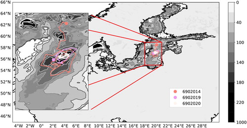
The floats have stayed relatively well in the deep areas of the Gotland Deep (Figure 1). The first float escaped from the area around May 2014. It escaped partly due to diving depth that was too low and partly due to the strong winds during the time.

Figure 1. Routes of the Argo floats near the Gotland Deep (left) and the location of the Gotland Basin on the Baltic Sea (right). The routes are identified by their WMO number. Topography data iowtopo2 (Seifert et al. 2001).

Usually the floats measured one profile per week. After deployments and in some high wind events, we changed to daily profiling to get better time resolution of the data and to keep control of the floats. On average, the diving depth within the study period was 160 m with a minimum of 100 m and a maximum of 210 m. The average diving depth was increased with each mission from 121 to 168 m, then to 203 m as we grew more experienced in operating the Argo floats.

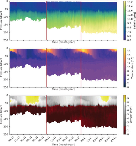
Data from the three missions was combined into one time series (Figure 2). From this series, we can see the seasonal stratification patterns, oxygen behaviour (Section 5.2) and inflow events (Section 5.1).

Figure 2. Measurements of the three Argo missions studied. Salinity (up), temperature (middle) and oxygen (bottom). Red lines indicate float changes.

3.2. Diving depth and bottom contacts

The mission profile depths, approximated bathymetry (Seifert et al. 2001), and float cycles with bottom contacts are shown in Figure 3. The average profile depth was increased from first to last mission by approximately 75 m, as can be seen in Figure 3. The grey areas show cycles with bottom contacts, and thus the profile depth at those times gives accurate bathymetry information. The bottom contacts were determined from the float's drifting data by assuming that if the float parking depth varies less than 0.05 m during 10 h, the float was at the bottom. The resolution of the reference bathymetry data used is about 1 nmi. On average, the distance between the float coordinates and the closest bathymetry grid point was 730 m. The float depth during the bottom contact mostly corresponds well with the closest bathymetric data.

Figure 3. Profile depth (solid lines) and approximated bathymetry along the float drift route (dashed lines) during different missions (colours). The shaded grey areas show float cycles with bottom contact at some point during the cycle. Bathymetry approximated from the Leibniz Institute for Baltic Sea Research (IOW) bathymetry dataset (Seifert et al. 2001).

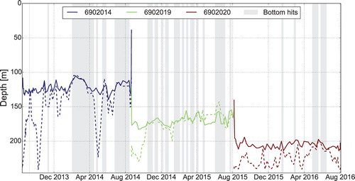
The number of bottom contacts changed considerably from one float to another. The First one managed to avoid them until it drifted to north to a shallower area. Of the 93 profiles, 24 had a bottom contact. The second mission had slightly more bottom contacts (23 of the 63 profiles). The float managed to rise from the bottom without problems after each contact, even if the general type of bottom in the area were muddy (Winterhalter et al. 1981, Figure 140a). With the experience gained from the first bottom contacts, the risk of getting stuck to the bottom was deemed minor in the float's operating area. Based on this, we decided to keep the float close to the bottom to prevent it from escaping from the desired area.

With the third mission, the diving depth was successfully chosen, preventing the float from drifting into areas that were too shallow. As such, it had bottom contact in only 8 of the 68 profiles.

During these missions, the practice of operating shallow Argo floats was developed and improved. With the increased knowledge of the float behaviour, we were able to keep the float deeper with every mission. The initial mission had an average diving depth of 121 m, the second 169 m and the third 204 m. Initially, we limited the diving depth as we were over-cautiously avoiding the bottom contacts. This led on the first mission to the escaping from the designated deep area, and thus a further need for shallower dives. With the second float, we increased the diving depth, which kept it in the deeper area, but it ended up having a considerable number of bottom contacts. In the third one, we increased the diving depth further, and thus managed to keep the float deep enough to stay in its designated area and thus having less bottom contacts, as it remained mostly in the deepest area.

3.3. Deployment and operating area

The floats were deployed and recovered during R/V Aranda's annual COMBINE monitoring cruises. The active float was recovered, and another float was put instead. All three floats were deployed at 5 km from the first deployment point (20${}^{\circ }$ 2' E 57${}^{\circ }$ 19' N).

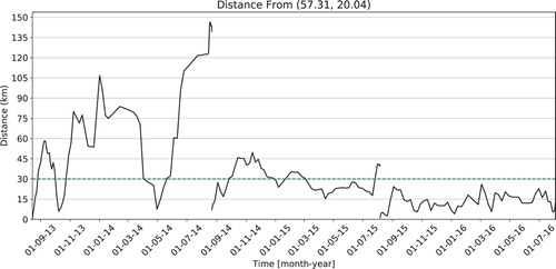
The distance of the floats from their original point of deployment can be seen in Figure 4. After staying in the area over half a year, the first float escaped the deployment area in May 2014, ending up over 100 km north from the point of deployment (see Figure 4). The other two floats stayed mostly within 40 km of the deployment point during their entire mission.

Figure 4. The distance of the float from the original deployment point as a function of time. The green line marks the 30 km distance.

3.4. Faulty measurements and quality control

The Coriolis data centre has quality-controlled the data on their system for consistency in for example timestamps and locations, and marked them with quality flags. For ocean profiles, Coriolis also performs numerous quality control steps (Carval et al. 2017), incompatible for the Baltic Sea, as the profiles differ considerably from the ocean profiles. As such, we removed faulty profiles with the quality control described below:

Most of the profiles were measured successfully. However, in some cases the CTD sensor had probably been clogged. These can be identified if either surface salinity exceeded 7.5 or if the salinity dropped quickly between two measurements. Here the limit of a quick sudden drop was set to 0.3 g/kg between two measurements if the following and previous measurement changes were less than 0.03 g/kg. This was set to not reject a profile with a strong halocline, as a real one would be visible in more than one consecutive measurement. In total, 12 out of 446 profiles (≈3%) were marked as flawed. This method detects clearly faulty profiles, but does not ensure all clogged measurements are detected, especially if the fault has been just temporal.

The recovered floats were sent back to the manufacturer where they were inspected, their sensors calibrated, maintenance-serviced, batteries replaced, and sent back to us so that we could deploy them again.

4. Argo data compared to other monitoring data

As Baltic Sea Argo floats are part of the global Argo program for monitoring the World Ocean, it is natural to reflect their data against the data from regular monitoring cruises of the Baltic Sea, which is done within the HELCOM cooperation. HELCOM has many monitoring programs, and from those we refer to the Cooperative Monitoring in the Baltic Marine Environment (COMBINE) and to the data that is publicly available from the ICES data centre as a dataset by the HELCOM area.

The COMBINE program has two types of observing stations: mapping stations and high-frequency stations (HELCOM 2017). The data consists of water sample data and CTD measurements collected by various countries and institutions. The HELCOM dataset is now maintained at the ICES data centre, and it includes data since 1898 from HELCOM monitoring stations listed in the ICES station dictionary (http://ices.dk/marine-data/tools/pages/station-dictionary.aspx). The mapping stations are visited only a couple of times per year, and the high-frequency stations are aimed at giving information on the annual course of the processes.

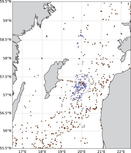
The HELCOM dataset is a subset of ICES CTD and bottle data, which also contains data from stations other than the HELCOM monitoring stations. That data is also publicly available from ICES. Because we wanted to compare our Argo data to data from ship observations as near to the Argo profiles as possible, we downloaded the relevant ICES data for our comparisons. Figure 6 shows the locations of CTD measurements in the ICES data and the locations of our Argo profiles studied here.

The most consistent fixed location time series from the Gotland Deep HELCOM monitoring station BY15 consists of on average two profiles per month during the Argo operational period (Figure 5). From the 1960s to the early 2000s the profiling frequency at BY15 increased from one to four profiles per month, after which it decreased to the present two per month. The Argo float profiles nearby the monitoring station therefore more than doubles the temporal data coverage there. This added frequency helps studying events taking days or weeks, like stratification, and increase the chances of getting measurements of shorter incidents like storm-induced mixing. In Section 5, we consider some of the phenomena detected.

Figure 5. Number of Argo and shipborne CTD profiles per month 30 km from HELCOM monitoring station BY15 (57.32 N 20.05 E) for the study period.

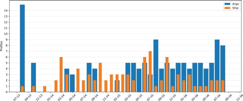
Figure 6. Locations of CTD profiles from ICES data (red stars) and Argo profiles (blue crosses) studied in this paper. The Most frequent measuring point, BY15 (57.32 N 20.05 E), which is also the starting point of all three Argo missions, is marked with a light red circle. The light blue circle marks the 30 km radius from the By15.

The advantage of the monitoring points, compared to the Argo measurement, is their consistency in place. With the Argo floats, we need to consider more of the drift in both time and location.

To validate Argo measurements against CTD, we searched the closest matches from both datasets both in time and location, and we checked how different the given results were on average. To determine the closest pair, we used the relative distance ($D_r$), which was determined as:(1) $D_r=D_{km}+3\frac{km}{d}\cdot D_d$(1) Where $D_{km}$ is the distance of measuring points in kilometres, and $D_d$ is their distance in days. 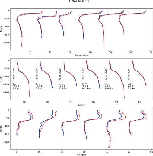The constant 3 was chosen for the equation after testing, as $3km/d$ is in the range of drifting speeds of the floats in the area, and it gave a reasonable compromise between distances in days and kilometres. Figure 7 shows examples of the best matches for the float 6902019.

Figure 7. Best CTD matches for Argo 6902019. Temperature (a), salinity (b) and oxygen(c) are represented. Red indicates CTD measurements, Blue Argo. Each profile is shifted 10 units on their respective x-axis from the next one. The date of the Argo measurement is next to each salinity profile. Numbers under the date indicate the relative distance from the ship CTD, distance in days and distance in km. Negative day difference indicates an Argo float measurement earlier than the ship CTD.

We got closer matches between the Argo float and ship profiles in later missions as we gained more experience in operating the floats. We managed to increase the average diving depth with each mission and thus keep the floats more confined, which increased the amount of concurrent ship CTDs, as the float stayed closer to the BY15.

Each Argo profile was paired with the closest (smallest $D_r$) ship CTD. This often means that the same ship CTD will be the best match for several Argo profiles, especially on occasions when the Argo float measured once a day, during deployment and pick-up. This would cause most of the best matches to describe the same situation, which is undesired. For this reason, for the pairs with the same ship CTD, we only picked for further analysis the one with smallest $D_r$. This left us with 18, 14 and 25 unique pairs for each mission. Of these, we picked for analysis the ones with $D_r<35.0$, leaving 6, 7 and 20 profiles, respectively (Table 2). The importance of the measuring point BY15 in the comparisons shows for the first mission 3 out of 6 selected missions is within 10 km of it, and for the second and third missions the same rates are 2 out of 7 and 19 out of 20, respectively.

Table 2. Comparison of the bias between ship CTD measurements and Argo floats. Profile pairs with $D_r<35$ were used for analysis. Lower values of the first float have been omitted, as none of its profiles reached the full 150 m depth.

Bias between CTD and Argo measurements
	Surface layer (0–30 m)			Bottom layer (80–150 m)
Float WMO	O${}_2$ (ml/l)	Salinity (g/kg)	T${}^{\circ }$C	O${}_2$ (ml/l)	Salinity (g/kg)	T${}^{\circ }$C	Pair No
6902014	0.3	−0.08	−0.66	–	–	–	6
6902019	1.1	−0.05	−0.10	0.17	0.05	0.03	7
6902020	0.6	−0.01	−0.06	0.19	−0.05	−0.01	20

The remaining pairs were used to get an idea of possible systematic bias in the measurements. The best matches for each float were less than two kilometres away and within a day; and for the last accepted, the higher distance was either under 10 days or 20 km. With these distances, single profiles can have considerable differences, but the average differences are interesting to look at.

The biases are listed in Table 2. The depth studied were divided into surface layer (0–30 m) and bottom layer (80–150 m). The in–between area (30–80 m) was omitted, as it is less homogeneous and as such would require taking into account the properties of the sensors in much more detail. In addition the changes in location and time are more dominant in this layer. The bottom layer data was discarded from the first float, as its average diving depth was 121 m, with no profiles covering the whole 80–150 m range.

Temperature and salinity differences between the Argo float and ship data are small, considering that the matches are not in exactly the same places or times. The biases are small, generally under 0.1${}^{\circ }$C. The first float has the highest bias of 0.7${}^{\circ }$C on the surface layer, with also the highest average differences in the measurements. This is partly due to it escaping the Gotland Deep to the north, where there were fewer profiles to match, partly for the number of comparable profile pairs being only 6.

The oxygen values in the upper layer in the first and last mission were 0.3–0.6 ml/l, and on the middle float about 1 ml/l lower than the corresponding CTD measurements. The manufacturer gives an accuracy of 5% for the sensor (Aanderaa Data Instruments AS 2001). In the surface layer, with O${}_2$ of 8–10 ml/l these differences are within expectations, taking into account the differences in place and time for the first and third mission; but for the second mission, the oxygen values are lower than expected. This can also be seen from Figure 2, as oxygen in summer 2015 is lower than others in the Argo float measurements. Such a difference cannot be seen in ship CTD measurements. It seems that based on this, there are differences in the oxygen calibrations on the floats, which should be taken into account.

5. Case studies in the Gotland Basin

To show the potential of the Argo data in the Baltic Sea monitoring and research, we briefly deal with two case studies. The first case in the major Baltic inflow that occurred in December 2014. The other case is related to process studies and deals with upper-layer mixing.

5.1. Detected Baltic inflow effects on oxygen and salinity

A Major Baltic Inflow occurred in 2014 December (Mohrholz et al. 2015; Holtermann et al. 2017). More saline, oxygen rich, inflowing waters flowed slowly north along the bottom or along certain density layers. The MBI became visible in the Gotland Deep after Feb 2015 (Schmale et al. 2016). The first half of 2015 was still in the middle of the learning curve of our Argo operations, and therefore our profiles did not reach the near bottom waters of the Gotland Deep. Holtermann et al. (2017) measured the oxic situation in the Gotland Sea at the Gotland Deep Environmental Sampling Station (GODESS) in 2015 and noticed the intrusion of the MBI-induced water masses at the bottom-most layer (around 200 m) in February 2015, with salinity and oxygen peaking at the end of April 2015.

In our Argo measurements, the changes in the deep water salinity and oxygen content became visible in mid-April 2015, as our profile depth at the time was around 170 m (Figure 8). The decay of the oxygen content in the intermediate deep waters is seen from September 2015 to March 2016. Another small rise in oxygen can be interpreted at the lowest depths from the data during March–May 2016.

Figure 8. Salinity and oxygen measurements at the time when the 2014 MBI reached the Gotland Deep. Red lines indicate float change.

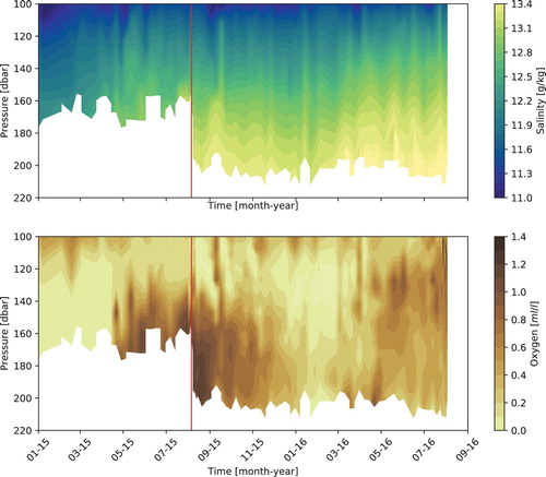
The zero level of the Argo oxygen sensors differed by roughly 0.1 ml/l. This is seen as a discontinuity in the time series at time points where the missions changed (Figure 9). The different calibration of the Argo floats was also visible in our analysis of the differences between the Argo float data and the ship data, with the differences between the missions the largest at the surface, roughly 0.5 ml/l (Table 2).

Figure 9. The salinity (above) and oxygen (below) as a function of time, from the Argo profiles, from 120, 150 and 180 m depths, where the float went deep enough. The change in salinity was slightly under 1 g/kg from both 120 and 150 m. The change was sharper at 150 m. Oxygen in 120 m rose at highest to 1 ml/l

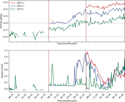
Figure 9 shows the change in salinity and oxygen at 120, 150 and 180 m depths during the MBI. The salinity at 120 m depth increased roughly by 0.5 g/kg from May 2014 to Feb 2015. Between February and March 2015 the salinity increased by approximately another 0.5 g/kg and then stabilised to 12.3 g/kg. At the same time, oxygen conditions changed from near zero to 0.8 ml/l by April 2015 at 120 m depth.

At 150 m depth, the Argo measurements started in July 2014. Salinity has been rather constant there until March 2015. Between March and May 2015, the salinity at 150 m depth increased rapidly by 0.6 to 12.6. The change in oxygen content was stronger at this depth, approximately 1 ml/l starting from April 2015. The peak oxygenation here was reached in July 2015 at nearly 1.1 ml/l. In the beginning of 2016, the oxygen vanished from this depth. At 180 m depth, we mainly got measurements from the last float. Both the salinity and oxygen there followed the same trends as at 150 m. These results are consistent with the results of Holtermann et al. (2017), considering that the float moves and that the lower-most layer is missing due to the diving depths, especially in earlier missions.

The Argo data from the Gotland Deep gives additional information on the MBIs and will give even more in the future when the routine operations have matured to catch a more complete column. The advantage is that if an MBI is identified by other means, we can increase the frequency of observations during the phase when the MBI reaches the Gotland Deep.

5.2. Wind-induced mixing in the surface layer

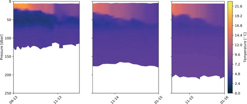
The Argo dataset that we analyse here covers three springs and three autumns. As the floats measure approximately one profile a week, the time scale fits well for monitoring the general spring and autumn stratification cycle. We can see both the formation and the decay of the thermocline during three years from the dataset (Figure 2).

For example in 2013, the thermocline eroded faster than in 2014 and 2015 (Figure 10), which was caused by the hurricane class storm ‘Christian’. The storm crossed the Baltic Proper along its pathway from southern Scandinavia to southern Finland on October 28, 2013. In Denmark, the wind speeds reached the classification of violent storm and the maximum 10 min average speed measured was 39.5 m/s at the Danish Meteorological Institute station number 615900, Røsnæs Fyr. From the 28th to the 29th of October, the wind speed was from 17.4 to 22.1 m/s at the Östergarnsholm weather station, on the Gotland island in Sweden. This is the closest weather station to the Argo Baltic Proper locations. The maximum significant wave height in the northern Baltic Proper wave buoy during that event was 5.2 m.

Figure 10. Autumn stratifications (2013, 2014 and 1015). At the far left (2013), the stratification dissolved quicker, due to hurricane ‘Christian’. White colour indicates no data.

The strong thermocline eroded between two Argo profiles measured on the 24th and 29th of October (Figures 10 and 11), and denser water seems to have entered the area. The total salinity increase from the profiles before the storm to after the storm is explained by the float drifting nearly 40 km south, where the salinity is higher.

Figure 11. Argo profiles of temperature (left) and salinity (right) before and after the hurricane class storm ‘Christian’.

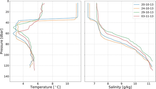
After the storm event, the thermocline started to re-establish until 20 November, after which it continued to deteriorate like in other autumns.

In 2014 and 2015, the thermocline erosion was not as dramatic as in 2013. These autumns were more calm, and the strong winds appeared later in the year when the stratification had already eroded due to the cooling of the water and milder weather events.

6. Discussion

Before the FMI's Argo missions in the Baltic Sea, the overall expectations of the possibility to operate them in marginal seas was rather pessimistic. The assumptions were that they most likely either get stuck on the bottom or drift to the shores pretty soon, before having time to do a proper measurement series. Luckily these expectations turned out to be too pessimistic, and now we are able to operate the Argo floats operationally in the Baltic Sea. Our operational Argo activity in the Gotland Deep has continued since the missions studied here with two floats (WMO numbers 6902024 and 6902027).

Operating an Argo float is relatively cheap in comparison to ship days: one Argo costs roughly as much as one ship day with a medium-sized, well-equipped research ship (National Research Council 2009; Argo project 2018, p. 68). The manpower needed during the Argo operations is small, and the work is done remotely. Ship-borne measurements and Argo operations are, however, very different in nature and will complement each other in the Baltic Sea: Research vessels can choose the exact time and location of the measurements and have a high depth resolution. A research vessel can also easily carry out a wide range of measurements on the same spot. The drawbacks are the limitations of hard weather and the cost of measuring. The ship's mission must also be planned far ahead, and changing weather can force the plans to change or be completely cancelled at worst. Argo floats are practically weather-independent and can measure frequently for long time periods. Their observation time step can be changed when needed, and the data is almost real-time. As Argo float profiles are usually recorded with constant intervals, it is likely to get profiles near before and after sudden events, occasionally even during them also in routine missions.

One drawback in our Argo data is the loss of the topmost metres of the surface layer. The algorithm that protects the SBE CTD sensor of our APEX floats shuts down the measurements well before the sensors reach the surface (Haavisto et al. 2018).

Argo floats are freely drifting platforms. In the Gotland Deep, the floats stayed most of the time within 30 km of the deployment point, occasionally drifting over 60 km away (Figure 4). As such, the whole dataset has profiles from a rather large area. The separation of temporal and spatial variations from the data needs to be considered carefully. To solve this problem, it is possible to select profiles according to the distance from a defined point for further time series analysis. This way, fewer profiles can be used in the analysis, but they are the ones which describe a similar area. This can be desired when comparing data with another, stationary system, or when the float circulates in an area with inhomogeneous properties to monitor the differences between these areas. It should also be kept in mind that Argo floats move with currents and can follow the movements of water masses. In contrast, shipborne CTD can be taken in the same spot regardless of the movements of water. With the float series, where new float replaces another, the jump in location and possibly also in calibration from one float to the another must be handled carefully (Figure 4).

The frequency of the Argo profiles makes it possible to monitor the evolution of the oxygen content for a longer period. The choice of the diving depth, however, is a compromise between the completeness of the profile down to the bottom and with the risk of losing the float in a bottom hit. Even with the cautious approach on the first missions described in this paper, the diving depths were enough to detect the major inflow event. With the improved understanding of how to operate Argo floats in the area, we will have even more complete data from the coming inflow events. As the oxygen measurements did have a higher bias than the CTD measurements, one should be careful when interpreting them.

Quality control of the Argo data needs further research when applied to marginal seas like the Baltic Sea. Consequent profiles can have large differences in salinities caused by a drifting of relatively small distances or strong salinity gradients. The well-established methods used in the large oceans can falsely flag these changes as measurement errors. In this work, we have presented a rudimentary method for detecting the faulty profiles, but further work is needed. Oxygen-sensor calibration needs further improvement. With the aid of close-by ship CTD measurements, it is possible to detect and account for the oxygen measurement bias. The procedures for doing this need to be further studied.

The tests in the Black Sea have found that the greater number of the Argo floats in the area had a larger impact on data assimilation quality than increasing the profiling frequency by the same amount (Grayek et al. 2015). The possibilities for increasing the number of Argo floats in the Gotland Deep are therefore studied. They are a very cost-efficient means of monitoring, and their use is agreed on within the IOC at least in the ocean. In the optimal case, several floats could be used after an MBI to more accurately measure the spread of the water masses.

The Argo floats applied in the Gotland Deep and the Baltic Sea in general can be used to study various cases other than the ones presented in this paper. In case of MBIs, the spreading of the incoming water is of interest, and then spatial variability is important. With enough Argo floats for longer time periods, the deep currents of the areas can also be researched (Roiha et al. 2018). Especially in the northern parts of the Baltic Sea, with proper ice avoidance, the possibility to measure under ice can provide valuable information that is hard to obtain in other ways. With a large enough fleet of Argo floats, modelling work on the Baltic Sea would also benefit through verification and assimilation of the Argo data. Occasional events, like Major Baltic inflows or storms, can be studied in more detail even with a regular weekly cycle of Argo floats. MBIs can be detected months before their effects arrive in the Gotland Deep. Because of this we can increase the Argo float measurement frequency in due time for the study of the coming MBIs at virtually no extra cost.

For further advancing the Argo measurements in the Baltic Sea, the controlling methods should be further developed and automated as the number of floats in operation increases. This requires developing algorithmic or artificial intelligence based control schemes and further study of the behaviour of the floats at given depths, areas and weather conditions. For northern parts, the application of ice-avoidance systems should be further advanced and studied with both algorithmic systems and physical solutions.

The topography plays an important role when planning further deployments of the Argo floats in marginal seas. Based on these experiences, the Gotland Deep is a suitable location, as it is relatively deep, and the deeper drift kept the float circulating around the area rather than moving it away. The size of the area confines the float to roughly a 40 km radius area, which is small enough to give meaningful local time series and large enough that weather fluctuations will not easily push it out of the area. Other basins with similar characteristics should be considered for further float deployments. Another larger area is operated in the Gulf of Bothnia (Haavisto et al. 2018; Roiha et al. 2018). Other interesting areas for deployment in the Baltic Sea include Bay of Bothnia, Gulf of Gdansk, Bornholm Basin (IOPAN 2018) and Western Gotland Basin. Poland is an observer at Euro-Argo, and the Institute of Oceanology of the Polish Academy of Sciences (IOPAS) in Sopot has begun to use Argo floats since November 2016 in the southern Baltic Sea including the Bornholm Basin. That data is also available at the Coriolis Argo data centre.

We study the options to keep the floats even closer to the bottom on certain occasions. Up to now the missions have followed a safety strategy with minimised risks of instrument losses and sensor faults. We have tried to guarantee the recovery of the floats by limiting the measurements in a way that the energy consumption is on the level where the float remains active until the next suitable research cruise for recovery. Webb Research specifications give 4 years and 150 ascents nominal operation capacity for the Apex float in the ocean with 2000 m profiling depth. With such specifications, about a one year mission time in the Gotland Deep is very feasible with one profile per week sampling.

Because the Argo floats are freely drifting devices, there is a concern about misinterpreting the data in respect to time and horizontal variations. There may be ways to decrease the danger of misinterpretations due to horizontal variations by using satellite data, though that data is surface data and Argo data is not, but mesoscale features may be identified from satellite images. The other way is to benefit from Alg@Line data, from where horizontal correlation scales can be estimated along the ship routes.

7. Conclusions

FMI has experimented with Argo floats in the Baltic Sea since 2011, first in the Bothnian Sea and then extended to the Gotland Deep. Operating the floats has matured to a level where we can state that Argo monitoring of the Baltic Sea is now an operative reality. The data goes in near real–time to the global Argo data centre and is available on the Internet. Finland is a member of Euro–Argo and has Argo floats in the North Atlantic, too. This membership should guarantee continuity of this operative monitoring and gives possibilities to develop the Baltic Sea monitoring. However, when operating in the area, the various national jurisdictions should be considered, especially as the Intergovernmental Oceanographic Commission's Executive Council adopted in June 2018 (IOC 2018) a decision that expands the standard bio-Argo float sensors to include oxygen, pH, nitrate, chlorophyll, backscatter and irradiance.

Operating Argo floats, which were originally planned for deep ocean use, in a shallow marginal sea is demonstrated to be feasible, cost-efficient and useful in the varying conditions in the Baltic Sea. It complements measurements done by other means like research ships, moored stations and gliders. The latter ones are coming to the Baltic Sea after Argo floats, as both Estonia and Finland are now using shallow water gliders there, too.

The Argo floats supplement well the data gathered from other instruments. The investment is relatively low cost. The floats are recoverable during regular monitoring cruises; they are reusable after maintenance; they are practically weather-independent; and the data comes in near real-time within an international data exchange system and is freely available. The telemetry costs are feasible and ‘piloting’ costs are rather low, too. Argo floats are meant to be autonomous without the need for piloting. However, in the Baltic Sea some ‘piloting’ guarantees they keep running in the desired areas. This means that their location must be monitored on a weekly basis, and there needs to be established practices to give them new instructions if needed. Since the floats studied here, we have constantly maintained at least one active Argo float in the Gotland Deep and various numbers of active Argo floats in the Bothnian Sea.

We have shown that the resolution of the measurements is capable of systematically detecting changes in the dynamics of the sea on the scale of days, for example the thermocline erosion in autumn 2013 during the hurricane class storm.

The effects of the late 2014 MBI was also detected in the Argo data. The first signs were seen in the deepest observations.

Argo floats detected the first signs of the late 2014 MBI around April, 2015, with increasing salinity and oxygen levels at the depths of 150 m. Around the same time, it was visible on CTD measurements that reached the bottom (235 m) (Neumann et al. 2017).

Acknowledgments

ICES Dataset on Ocean Hydrography. The International Council for the Exploration of the Sea, Copenhagen. 2014 Argo data was collected and made freely available by the International Argo Program and the national programs that contribute to it. (http://www.argo.ucsd.edu, http://argo.jcommops.org). The Argo Program is part of the Global Ocean Observing System.

Disclosure statement

No potential conflict of interest was reported by the authors.

ORCID

Simo Siiriä http://orcid.org/0000-0001-8261-8370

Petra Roiha http://orcid.org/0000-0001-9585-206X

Laura Tuomi http://orcid.org/0000-0003-2471-6815

Pekka Alenius http://orcid.org/0000-0002-8033-4830

References

- Aanderaa Data Instruments AS. 2001. Oxygen optode. [accessed 2018-03-20]. https://www.aanderaa.com/media/pdfs/oxygen-optode-4330-4330f.pdf.
- Argo project. 2018. Argo, part of the integrated ocean observation strategy. [accessed 2018-06-06]. http://www.argo.ucsd.edu/FAQ.html#cost.
- IOPAN. 2018. Baltic Argo floats deployed by IO PAN. https://www.iopan.pl/hydrodynamics/po/Argo/argo.html.
- Carval T, Keeley R, Takatsuki Y, Yoshida T, Loch S, Schmid C, Goldsmith R, Wong A, McCreadie R, Thresher A, et al. 2017. Argo user's manual v3.2.
- Coriolis. 2001. Coriolis data portal. [accessed 2017 Sep 7]. http://www.coriolis.eu.org/.
- Dietze H, Löptien U. 2016. Effects of surface current/wind interaction in an eddy-rich general ocean circulation simulation of the Baltic Sea. Ocean Sci. 12:977–986. http://oceanrep.geomar.de/31634/. doi: 10.5194/os-12-977-2016
- Grayek S, Stanev EV, Schulz-Stellenfleth J. 2015. Assessment of the Black Sea observing system. A focus on 2005-2012 Argo campaigns. Ocean Dyn. 65(12):1665–1684. https://doi.org/10.1007/s10236-015-0889-8.
- Haavisto N, Tuomi L, Roiha P, Siiriä SM, Alenius P, Purokoski T. 2018. Argo floats as a novel part of the monitoring the hydrography of the Bothnian Sea. Front Mar Sci. 5:324. https://www.frontiersin.org/article/10.3389/fmars.2018.00324.
- Holtermann PL, Prien R, Naumann M, Mohrholz V, Umlauf L. 2017. Deepwater dynamics and mixing processes during a major inflow event in the central Baltic Sea. J Geophys Res Oceans. 122(8):6648–6667. http://dx.doi.org/10.1002/2017JC013050.
- National Research Council. 2009. Science at sea: meeting future oceanographic goals with a robust academic research fleet. Washington (DC): The National Academies Press. https://www.nap.edu/catalog/12775/science-at-sea-meeting-future-oceanographic-goals-with-a-robust.
- IOC. 2018. Intergovernmental oceanographic commission: fifty-first session of the executive council, draft summary report, Part 2. http://ioc-unesco.org.
- IOC, SCOR, IAPSO. 2010. The international thermodynamic equation of seawater – 2010: calculation and use of thermodynamic properties. UNESCO. (Intergovernmental Oceanographic Commission, Manuals and Guides; 56).
- Leppäranta M, Myrberg K. 2009. Physical oceanography of the Baltic Sea. Berlin, Heidelberg: Springer-Verlag.
- Le Traon PY. 2013. From satellite altimetry to Argo and operational oceanography: three revolutions in oceanography. Ocean Sci. 9:901–915. doi: 10.5194/os-9-901-2013
- HELCOM. 2017. Manual for marine monitoring in the COMBINE Programme of HELCOM. http://www.helcom.fi/action-areas/monitoring-and-assessment/manuals-and-guidelines/combine-manual/.
- Matthäus W. 2006. The history of investigation of salt water inflows into the Baltic Sea–from the early beginning to recent results. Rostock-Warnemünde: Inst. für Ostseeforschung.
- Meier HEM, Feistel R, Piechura J, Arneborg L, Burchard H, Kuzmina N, Mohrholz V, Nohr C, Paka VT, Sellschopp J, et al. 2006. Ventilation of the Baltic Sea deep water: a brief review of present knowledge from observations and models. Oceanologia. 48(S):133–164.
- Mohrholz V, Naumann M, Nausch G, Krüger S, Gräwe U. 2015. Fresh oxygen for the Baltic Sea – an exceptional saline inflow after a decade of stagnation. J Mar Syst. 148:152–166. http://dx.doi.org/10.1016/j.jmarsys.2015.03.005.
- Neumann T, Radtke H, Seifert T. 2017. On the importance of major Baltic inflows for oxygenation of the central Baltic Sea. J Geophys Res Oceans. 122(2):1090–1101. http://dx.doi.org/10.1002/2016JC012525.
- Prien RD, Schulz-Bull DE. 2016. Technical note: godess – a profiling mooring in the Gotland Basin. Ocean Sci. 12(4):899–907. https://www.ocean-sci.net/12/899/2016/. doi: 10.5194/os-12-899-2016
- Purokoski T, Aro E, Nummelin A. 2013. First long-term deployment of Argo float in Baltic Sea. Sea Technol. 54:41–44.
- Riser SC, Freeland HJ, Roemmich D, Wijffels S, Troisi A, Belbéoch M, Gilbert D, Xu J, Pouliquen S, Thresher A, et al. 2016. Fifteen years of ocean observations with the global Argo array. Nat Clim Chang. 6(2):145. doi: 10.1038/nclimate2872
- Roiha P, Siiriä SM, Haavisto N, Alenius P, Westerlund A, Purokoski T. 2018. Estimating currents from Argo trajectories in the Bothnian Sea, Baltic Sea. Front Mar Sci. 5:308. https://www.frontiersin.org/article/10.3389/fmars.2018.00308.
- Schmale O, Krause S, Holtermann P, Guerra NCP, Umlauf L. 2016. Dense bottom gravity currents and their impact on pelagic methanotrophy at oxic/anoxic transition zones. Geophys Res Lett. 43(10):5225–5232. https://agupubs.onlinelibrary.wiley.com/doi/abs/10.1002/2016GL069032.
- Seifert T, Tauber F, Kayser B. 2001. A high resolution spherical grid topography of the Baltic Sea – 2nd ed. Baltic Sea Science Congress, Stockholm Nov 25–29, Poster #147. www.io-warnemuende.de/iowtopo.
- Tuomi L, Myrberg K, Lehmann A. 2012. The performance of the parameterisations of vertical turbulence in the 3D modelling of hydrodynamics in the Baltic Sea. Cont Shelf Res. 50:64–79. doi: 10.1016/j.csr.2012.08.007
- Westerlund A, Tuomi L. 2016. Vertical temperature dynamics in the northern Baltic Sea based on 3D modelling and data from shallow-water Argo floats. J Mar Syst. 158:34–44. http://www.sciencedirect.com/science/article/pii/S0924796316000191. doi: 10.1016/j.jmarsys.2016.01.006
- Winterhalter B, Flodén T, Ignatius H, Axberg S, Niemistö L. 1981. Chapter 1. Geology of the Baltic Sea. In: Voipio A, editor. The Baltic Sea. Elsevier; p. 1–121. (Elsevier oceanography series; vol. 30). http://www.sciencedirect.com/science/article/pii/S0422989408701387.