Interpolated fields of satellite-derived multi-algorithm chlorophyll-a estimates at global and European scales in the frame of the European Copernicus-Marine Environment Monitoring Service

ABSTRACT

The new level-4 daily chlorophyll-a interpolated products described in this paper and freely available in the Copernicus-Marine Environment Service, aim at providing daily continuous fields (cloud-free) of satellite-derived chlorophyll-a surface concentration at two different resolutions: 4*4 km over the world and 1*1 km resolution over Europe. The multi-sensor daily analyses, by filling the cloudy pixels, provide high-frequency retrievals of chlorophyll-a which can contribute to a better monitoring of the phytoplankton biomass. From a methodological point of view our approach is a combination of a water-typed merge of chlorophyll-a estimates and an optimal interpolation based on the kriging method with regional anisotropic covariance models. These analysed products have been designed to meet the expectations of the end users, by considering both the typical lack of observations during cloudy conditions and the historical multiplicity of available algorithms involved by case 1 (oligotrophic) and case 2 (turbid) water classifications. These products gather MODIS (Moderate Resolution Imaging Spectroradiometer), MERIS (MEdium Resolution Imaging Spectrometer), SeaWiFS (Sea-viewing Wide Field-of-view Sensor), VIIRS (Visible Infrared Imaging Radiometer Suite) and OLCI (Ocean and Land Colour Instrument) daily observations from 1997 to the present. A total product uncertainty, i.e. a combination of the interpolation and the product error, is provided for each pixel.

1. Introduction

In the ocean colour chain, observations from the Top Of Atmosphere (TOA), i.e. the level 1 products, are firstly corrected for the atmospheric signal using a specific method for each sensor to obtain the level 2 products, i.e. water leaving reflectances or radiances (Antoine and Morel 1999; Wang 2010; Saulquin et al. 2016). Given the level 2 products, oligotrophic case 1 (Bricaud et al. 1998; Loisel and Morel 1998; O’Reilly et al. 2000; Morel et al. 2006, 2007) or regional case 2 algorithms, for coastal turbid waters, are used to estimate the water constituent properties such as chlorophyll-a (chl-a) concentration, suspended matter concentration or the coloured dissolved organic matter absorption (Sathyendranath 2000; Doxaran et al. 2002; Siegel et al. 2005; Bowers and Binding 2006; Lee 2006; Doerffer and Schiller 2007; Saulquin et al. 2013, 2015). The multiplicity of both the atmospheric correction processors and the different algorithms used to estimate the same water constituents typically lead to a large number of available products for ocean colour. Another issue for users is that the sea surface observation in the optical range is not possible during cloudy conditions. As a consequence of all these issues, in many cases, scientists use monthly or weekly temporal composites of a specific chl-a product (case 1 or 2) that poorly address the real variability of the estimated parameter. We propose here daily analyses of satellite-derived surface chl-a concentration. The chl-a analyses involve multiple sensors, available since 1997, multiple chl-a algorithms and an interpolation scheme based on the kriging method using anisotropic covariance models. Such a daily space–time interpolation scheme is already available for Sea Surface Temperature (SST, Donlon et al. 2012) and Sea Surface Height (SSH, Schaeffer et al. 2011). However few experiments exist for ocean colour (e.g. Krasnopolsky et al. 2016) and this product is the first operational one at global scale, following the evolution towards multi-sensor products directly available to the user community as promoted by the Ocean Colour Climate Change Initiative of ESA (Melin et al. 2017).

Conversely to the standard daily, single sensor and single algorithm level 2 or level 3 products, the proposed level 4 products avoid end users having to consider both the typical lack of data (outside of the satellite swath or observed during cloudy conditions) and the historical multiplicity of available chl-a algorithms. Compared to our first version of the level 4 for the MyOcean project (Saulquin et al. 2010), precursor of the CMEMS, we introduced the optimal merging of different chl-a algorithms and an improved interpolation scheme with anisotropic covariance models near the coasts. The method is also now applied at global scale and a total uncertainty is provided with each pixel. Table 1 gathers the main characteristics of the products and Figures 1 and 2 show two examples of daily interpolated fields freely distributed in the frame of the Copernicus Marine Environment Monitoring Service (CMEMS).

Figure 1. Example of the OCEANCOLOUR_ATL_CHL_L4_NRT_OBSERVATIONS_009_037 daily L4 chl-a product for 20160801.

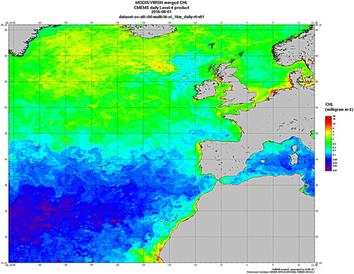
Figure 2. Example of the OCEANCOLOUR_GLO_CHL_L4_NRT_OBSERVATIONS_009_033 daily L4 chl-a product for 20160801.

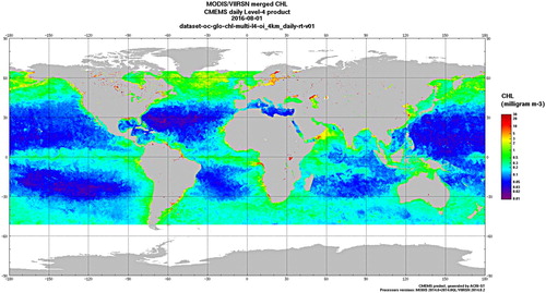
Table 1. Summary of the main characteristics of the L4 daily analysed chl-a products provided in the frame of the CMEMS for the global ocean and the European North-West Shelf Seas. Registration is required to freely access the data. J0 is the day of acquisition.

		CMEMS product reference (link to access)	Period	Availability	Used sensors
Near Real Time (NRT)	GLOBAL 4 km	OCEANCOLOUR_GLO_CHL_L4_NRT_OBSERVATIONS_009_033/	[2015-present]	J0+1, updated at J0+9	MODIS, VIIRS and OLCI^6
	ATLANTIC 1km	OCEANCOLOUR_ATL_CHL_L4_NRT_OBSERVATIONS_009_037	[2012-present]	J0+1, updated at J0+9	MODIS, VIIRS and OLCI^6
Reprocessing (REP)	GLOBAL 4 km	OCEANCOLOUR_GLO_CHL_L4_REP_OBSERVATIONS_009_082	[1997–2016]	n.a.	MODIS, MERIS, SeaWiFS, VIIRS and OLCI^6
	ATLANTIC 1 km	OCEANCOLOUR_ATL_CHL_L4_REP_OBSERVATIONS_009_098	[1997–2016]	n.a.	MODIS, MERIS, SeaWiFS, VIIRS and OLCI^6

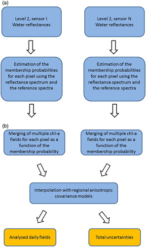
Figure 3 shows a synthetic flow diagram describing the two-step algorithm involved for processing the chl-a analyses. The first step aims at merging chl-a fields estimated using different algorithms, starting from the level 2 reflectances. The qualification of each algorithm has been performed in a previous validation step using an independent in-situ dataset (cf. §2.2). The aim of this probabilistic merging is to provide to end-users the ‘best’ estimate of the chl-a concentration for the observed pixel depending on the local conditions. The second step consists in a space–time interpolation of the chl-a merged fields of each sensor. Our interpolation technique is an advanced version of the standard optimal interpolation technique (OI) that includes anisotropic covariance models (Matheron 1971; Saulquin et al. 2010; Tandeo et al. 2014).

Figure 3. Synthetic flow diagram for the L4 products.

2. Methodology

2.1. Multi-algorithm merging to optimise chl-a estimates for a single pixel

We test in this study the suitability of the most popular chl-a algorithms for different types of water, typically the oligotrophic waters, the chl-a dominated waters and the coastal turbid waters. We have characterised in a first step the water types using the shape of in-situ radiometric spectra. To estimate the reference shapes, we used 7952 in-situ spectra, extracted from the MERMAID database (see annex 1) and an updated version of the k-means algorithm (Flannery 2007). The MERMAID dataset gathers more than 30 independent datasets, including the NOMAD and AERONET-OC datasets. Each spectrum is defined using 6 wavelengths: 412, 442, 490, 510, 555 and 670 nm. These in-situ measurements have been acquired all over the world and the sampling is considered here to be large enough to characterise the three selected water types (a minimum of 1,000 spectra was assigned to the smaller class). The metric used in the segmentation procedure is the mean spectral angle $\theta \left(i|k\right)$ between the k^th reference and the observed spectrum for pixel i (Kuching 2007):(1) $\theta \left(i|k\right)=\mathrm{arcos}\left(\frac{{\sum }_{\lambda }s{p}_i\left(\lambda \right)\ast sp\mathrm{\_}re{f}_k\left(\lambda \right)}{\left|s{p}_i\right|\ast \left|sp\mathrm{\_}re{f}_k\right|}\right)$(1) Where λ is the wavelength. 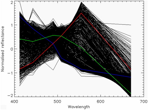|$s{p}_i$| and |$sp\mathrm{\_}re{f}_k$| are respectively the norm of the observed spectrum and the k^th reference spectrum (i.e. oligotrophic, chl-a dominated or turbid waters). Conversely to the approach proposed by Moore et al. (2001), our metric in (1) is only sensitive to the shape of the spectra and not the amplitude. The in-situ normalised spectra and the estimated reference spectra are shown in Figure 4.

Figure 4. The 3 normalised reference spectra estimated to characterise the water types. In blue, the reference shape for the clear oceanic waters. In green, the reference shape for the chl-a dominated waters. In red, the reference shape for the coastal waters influenced by suspended matters, chl-a and cdom absorption. In black, the spectrum database used to estimate the reference spectra with the updated k-means procedure.

The posterior membership probability of the observed spectrum at pixel i to the reference water type k is estimated as:(2) $P\left(i=k\right)=\frac{\theta {\left(i|k\right)}^{-1}}{{\sum }_{k=1}^N\theta {\left(i|k\right)}^{-1}}$(2)

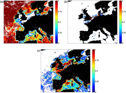
The posterior membership probability is thus estimated for all pixels and each sensor using the level 2 satellite-derived reflectance data in the first step of the processing (cf Figure 3). Figure 5 shows an example of the estimated spatial distribution of the observed water types using the MODIS Level 2 data for the month of March 2010 and eq. 2. To ensure the spatial continuity of the estimated chl-a merged fields, i.e. avoid zero to one probability switch, the merging between algorithms is performed using the membership probability weighted sum:(3) $\mathrm{Chla}\left(i\right)=\sum _{k=1}^{\mathrm{ncluster}}P\left(i=k\right).\mathrm{Chla}\left(k\right)$(3) (4) $\mathrm{With}:\sum _{k=1}^{\mathrm{ncluster}}P\left(i=k\right)=1,\mathrm{\forall }i$(4) Where $\mathrm{Chla}\left(k\right)$ is the estimated chl-a concentration for pixel i using the k^th algorithm.

Figure 5. The spatial distribution of the different water types observed in March 2010 using the MODIS data and eq. 2. Top, left, clear oceanic waters; top, right, chl-a dominated waters, bottom, coastal waters influenced by the suspended matters, chl-a and cdom absorption. White areas mean zero probability.

2.2. Interpolation methodology applied to the chl-a fields: the regional kriging with anisotropic covariance models at the shore

2.2.1. From isotropic to anisotropic covariance models in the optimal interpolation procedure

The interpolated variable is the chl-a anomaly for each sensor with respect to a global daily climatology computed at global scale using the chl-a merging technique and all sensors available (1997–2010). The isotropic distribution of the chl-a anomalies is an assumption that clearly fails in coastal areas where the coastal gradients are not constant in time and space. The chl-a analyses involve therefore anisotropic covariance models in the 0–200 km range from the shore. Conversely to the isotropic covariance models that state that the covariance only depends on the distance between two observations, the anisotropic model states that the covariance is a 2D function (e.g. the covariance follows gradient isolines near the shores). We use here two parameters to modify our initial interpolation scheme based on the isotropic hypothesis (Saulquin et al. 2010) to integrate the anisotropic hypothesis: the anisotropic ratio that estimates the local level of anisotropy, and the direction of the main covariance axis (see Tandeo et al. 2014, Figure 2, for the definition of a 2D semi-empirical variogram).

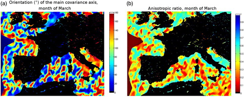
The estimation of both the local main covariance axis direction and the anisotropic ratio contribute to a better interpolation by first seeking for observations along the principal axis of covariance and second, by giving more important weights in the interpolation to the observations close to the main covariance axis. Figure 6 shows the monthly climatological anisotropic ratio (right) and the direction of the main covariance axis (left) for the month of March. An anisotropic ratio equal to 1 is equivalent to the isotropic situation, i.e. the covariance of the chl-a anomalies is independent of the direction and depends only on the distance (Matheron 1971; Saulquin et al. 2010).

Figure 6. Left, climatological orientation of the main covariance axis ϕ of the chl-a anomalies over European seas and the month of March (the zero is in the East direction). Right, climatological anisotropic ratio of the chl-a anomalies over European seas and the month of March.

Our operational interpolation scheme is thus based on maps of climatological monthly means for the variogram parameters, namely ${\sigma }_i$ the local sill for pixel i, px_i and pt_i respectively the local spatial and temporal nuggets, spatial_range_i and temporal_range_i respectively the local estimates of the maximum distance and time between two observations significantly correlated, ϕ_i the direction of the main covariance axis and ratio_i, the anisotropic ratio (see Saulquin et al. 2010 and Tandeo 2014 for details). These maps have been computed in a previous step using a regular grid of 0.15*0.15° resolution and the MODIS 2006–2013 training dataset. We introduce here the formalism used to update the classical spherical variogram to take into account the anisotropy. The experimental semi-variogram, ${\gamma }_{\mathrm{i}}\left({\mathrm{d}}_{\mathrm{t}},{\mathrm{d}}_{\mathrm{s}}\right)$, is obtained using the following equation applied to n(d_s, d_t) observations (chl-a anomalies) separated from distance d_s and time d_t (Matheron 1971; Saulquin et al. 2010):(5) ${\gamma }_{\mathrm{i}}\left({\mathrm{d}}_{\mathrm{t}},{\mathrm{d}}_{\mathrm{s}}\right)={\sigma }_{\mathrm{i}}\left(1.5\mathrm{d}-0.5{\mathrm{d}}^3\right)+\mathrm{p}{\mathrm{x}}_{\mathrm{i}}+\mathrm{p}{\mathrm{t}}_{\mathrm{i}}$(5) Where d is the spatio-temporal distance:(6) $\mathrm{d}=\sqrt{\frac{{\mathrm{d}}_s}{\mathrm{spatial}\mathrm{\_}\mathrm{rang}{\mathrm{e}}_{\mathrm{i}}}+\frac{{\mathrm{d}}_t}{\mathrm{temporal}\mathrm{\_}\mathrm{rang}{\mathrm{e}}_{\mathrm{i}}}}$(6) ${\mathrm{d}}_s$ is the Euclidian distance between two observations, ${\mathrm{d}}_t$ is the time interval. In case of anisotropic covariance, i.e. a ratio smaller than 1, the spatial distance ${\mathrm{d}}_s$ of eq. 6 is weighted using the anisotropic ratio and direction:(7) ${\mathrm{d}}_{\mathrm{aniso}}=\frac{{\mathrm{d}}_s\sqrt{\mathrm{rati}{\mathrm{o}}_{\mathrm{i}}}}{\sqrt{{\cos }^2\left({\varphi }_i\right)+\mathrm{rati}{\mathrm{o}}_{\mathrm{i}}{\sin }^2\left({\varphi }_i\right)}}$(7)

2.3. Total uncertainty associated with the CMEMS L4 chl-a daily products

The L4 chl-a analyses are provided with a total uncertainty in mg.m⁻³, ${\sigma }_i$, for each pixel n. ${\sigma }_i^2$ is expressed as the quadratic sum of the interpolation and the product errors:(8) ${\sigma }_i=\sqrt{{\sigma }_{i\mathrm{products}}^2+{\sigma }_{i\mathrm{interpolation}}^2}$(8) ${\sigma }_i\mathrm{interpolation}$ is the classical kriging variance (Saulquin et al. 2010)_: (9) ${\sigma }_{i\mathrm{interpolation}}^2=-\sum _{l=1}^n\sum _{j=1}^n{\lambda }_l{\lambda }_j\gamma \left(x_l,t_l;x_j,t_j\right)+2\sum _{l=1}^n{\lambda }_l\gamma \left(x_l,t_l;x_i,t_i\right)$(9) With $l$ and j the couples of observations used in the estimation of the interpolated value at pixel i.

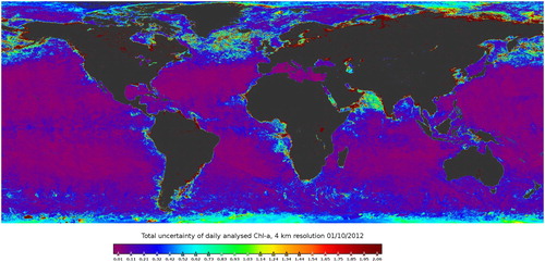
${\sigma }_i\mathrm{products}$ is the weighted sum of the uncertainty for each water type σ_k:(10) ${\sigma }_{i\mathrm{products}}=\sqrt{\sum _{k=1}^{\mathrm{ncluster}}P\left(i=k\right){\sigma }_k^2}$(10) P(i = k) is the membership probability of the spectrum at pixel i to the k^th reference water type, estimated using Eq. 2. σ_k is the chl-a k^th product uncertainty, estimated in a previous step using in-situ data (see §2.2 for the validation of the selected chl-a algorithms per water type) (Figure 7 shows an example of the total uncertainty provided for each pixel and the Level 4 products for the 01 October 2012.).

Figure 7. An example of the total chl-a uncertainty, in mg.m⁻³, provided with the chl-a L4 daily analysed fields (cf Eq 8). The stripes, or spatial discontinuities in the total uncertainty, refer to the observation temporal distribution: if some observations are available for the current day, the interpolation error term is lower leading to a lower total uncertainty.

3. Results of the validation of the chl-a fields

3.1. Protocol for the validation with matchups

The Copernicus-GlobColour products include comparisons between the MERIS, SeaWiFS, MODIS Aqua and VIIRS products and multiple in-situ datasets available in MERMAID (see Annex 1). The Principle Investigators (PI) are here duly acknowledged for providing these in-situ measurements. To establish the matchups, i.e. collocated observations in time and space between satellite observations and in-situ, the following protocol described here is used. The time difference between the in-situ record and the satellite overpass should not exceed ±12 h. For buoys/stations (where many in-situ measurements can be available) only the nearest in time is kept. A minimum of 10 valid pixels in a 5 × 5 pixel box centred on the in-situ location is required. Valid pixels means pixels for which no flag is raised (including clouds, ice, hilt, straylight, clouds, highglint, sensor zenith angle greater than 60^o, sun zenith angle greater than 70°, see SeaWiFS Postlaunch Technical report series 2003; MERIS Level 2 DPM 2011). For all the statistics, we used the reprocessed (REP) dataset. All the statistics are here computed the natural unit for the chl-a (no log-transformation).

3.2. Validation of the satellite-derived chl-a algorithms per water type

The tested chl-a algorithms were OC3 (Antoine and Morel 1999), GSM (Siegel et al. 2005), AP2 (Doerffer and Schiller 2007), and OC5 (Gohin et al. 2002). The statistical indices are ordered using their importance: number of matchups, bias, correlation coefficient and standard deviation. Underlined results highlight the ‘best’ algorithm for the considered water type. Table 2 confirms that the selected chl-a algorithms perform differently depending on the water type. This simple analysis justifies the merging approach of the chl-a estimates. Using the validation results in Table 2, for each water type, the following chl-a algorithms were selected for the creation of the level 3 multi-algorithm product used as input for the interpolation procedure (cf §1.1): clear oligotrophic waters, OC3; chl-a dominated waters, OC3; coastal waters, OC5. This qualification has been recently confirmed in Tilstone et al. (2017).

Table 2. Qualification of the most popular chl-a algorithms per water type. The ‘best’ algorithm is underlined for each water type I (results are estimated using the chl-a in mg.m⁻³).

	Clear waters	chl-a dominated waters	Coastal waters
OC3V5 (nb, bias, r², σ)	123, −0.004, 0.83, 0.18	239, −0.03, 0.81, 0.27	471, 0.16, 0.62, 0.25
GSM (nb, bias, r², σ)	117,0.002, 0.82, 0.18	204, −0.06, 0.74, 0.39	195, −0.27, 0.39, 0.45
AP2, MERIS neural network (nb, bias, r², σ)	124, −0.048, 0.49, 0.26	239, −0.14, 0.58, 0.37	475, 0.18, 0.63, 0.32
OC5 (nb, bias, r², σ)	124, 0.11, 0.77, 0.20	239, −0.04, 0.79, 0.29	475, 0.1, 0.67, 0.24

3.3. Validation of the water-typed chl-a merge (level 3) and the analysed fields (level 4)

Figure 8 shows the distribution of errors for the Global (4km resolution, top) and European products (1km resolution, bottom). On the left are shown the water-typed chl-a merged product validation (without interpolation) and on the right the corresponding interpolated products.

Figure 8. Histograms of the errors in mg.m⁻³ of the water-typed merge of chl-a (left) and interpolated fields (right) compared with in-situ chl-a measurements for (top) the global 4 km resolution products (033 & 082), and (bottom) the European 1km resolution products (037 & 098).

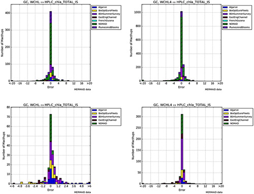
Table 3 provides a synthesis of the validation results with N the number of matchups, r, the Pearson correlation coefficient, slope and offset of the regression estimated vs in-situ, mean bias and standard deviation. Note that the interpolated products showed similar results to the non-interpolated products when the observation is available (i.e. when no interpolation is needed).

Table 3. Estimated accuracy statistics of the validation of the level 4 chl-a products (results are estimated using the chl-a in mg.m⁻³).

Variable (dataset)	N	r²	Slope	Offset	Bias	σ
All available matchups
chl-a analysis ATL 1 km resolution	500	0.81	0.78	0.05	0.07	0.29
chl-a analysis GLOB 4 km resolution	1765	0.81	0.85	0.01	0.02	0.28
chl-a water-typed merge (not interpolated) ATL 1 km resolution	119	0.82	0.79	0.03	0.05	0.27
chl-a water-typed merge (not interpolated) GLOB 4 km resolution	706	0.84	0.87	0.01	0.01	0.27
Interpolated data only (when no observation is available)
chl-a analysis ATL 1 km resolution	381	0.80	0.78	0.05	0.07	0.30
chl-a analysis GLOB 4 km resolution	1059	0.82	0.82	0.02	0.02	0.29

4. Conclusions

The observed differences in the performances of the four selected chl-a algorithms on three different water types (oligotrophic, chl-a dominated and coastal turbid) justified the water-typed merging of the chl-a estimates. The algorithm merging is performed for each pixel using a probabilistic approach based on the spectral mean angle between the observed spectrum and the three reference water types. The aim of this merging is to provide to end-users the ‘best’ estimate of the chl-a concentration for the observed pixel depending on the local conditions. In the near future, new algorithms will be evaluated, such as the one proposed by Hu et al. (2012) for oligotrophic waters, and included to either replace a selected algorithm for a specific type of water or address a new water type contributing hence to the continuous enhancement of the level 4 products for end users.

The spatio-temporal interpolation is performed using an optimal interpolation involving an anisotropic covariance model at the shore for a better reconstruction of the coastal gradients. The daily analysed fields are available since 1997. Compared with the multiple single sensor level 2 or level 3 products available in the CMEMS catalogue the approach proposed here simplifies the use of ocean-colour products and limits the number of datasets to be downloaded: the users do not have to take into account case 1 and case 2 issues anymore, nor cloudy conditions.

Results of the chl-a analyses validation exercise show a comparable quality, in term of bias and standard deviation, between the water-typed merged fields of chl-a and the corresponding interpolated products. We observe at the same time a multiplication by about 2.5 of the number of available matchups. Comparisons with in-situ data for the chl-a analysed global product show a low bias of 0.02 mg.m−3 with a coefficient of determination (r²) of 0.81. A total uncertainty, i.e. a combination of interpolation and product errors, is also provided for each daily product pixel. The CMEMS L4 daily chl-a products are freely available at a global scale at 4 km resolution (product id 009_033 & 009_082) and on the European North-West Shelf Seas at 1km resolution (product id 009_037& 009_098).

Acknowledgements

This work has been financed by the E.U. Copernicus Marine Service Information http://marine.copernicus.eu/. Thanks to Leanne Fraser, ARGANS, for reviewing the English.

Disclosure statement

No potential conflict of interest was reported by the authors.

Additional information

Funding

This work was supported by Copernicus Marine (CMEMS) [77-CMEMS-TAC-OC].

Annex: List of the in-situ datasets used for the validation

AAOT (AERONET-OC)	Giuseppe Zibordi	North Adriatic Sea 45.314N 12.508E
Abu Al-Bukhoosh (AERONET-OC)	Giuseppe Zibordi	Arabian Gulf 25.49N 53.14E
Algarve	John Icely	Sagres, Portugal 36/37N 8W
BioOptEuroFleets	Giuseppe Zibordi (ρw) J.F Berthon (IOP) Elisabetta Canuti (Chl)	Black Sea 42/45N 37/31E
BOUSSOLE	David Antoine	W. Mediterranean 43.367N 7.9E
Bristol Channel and Irish Sea	David McKee	Bristol Channel & Irish Sea 51/54N −3/-4E
BSH	BSH	North Sea
BSHSummerSurvey	Holger Klein	North sea English Channel 49.0/62.5N −6.0/8.25E
CALCOFI	CALCOFI PI^a	California
CaliforniaCurrent	Greg Mitchell Mati Kahru	California 32.2/34.8N 120.3/123.8W
CASES	Simon belanger Selima Ben Mustapha	Beaufort Sea 69.52/71.96N 123.22/138.93W
ChesapeakeBay	Michael Ondrusek	Chesapeake Bay 38.70/39.00N −76.30/.76.50W
CoveSEAPRISM (AERONET-OC)	Greg Schuster Brent Holben	Chesapeake Lighthouse 36.90N 75.71W
DYFAMED	Funding projects: EUROSITES (grant 202955), MOOSE, EMSO and FIXO3 (grant 312463).	Mediterranean NW Pacific Tropical South
EastEngChannel	Hubert Loisel	Eastern English channel 49.4/51.4N 0.0/3.0E
FrenchGuiana	Hubert Loisel	French Guiana 4.7/5.0S 51.9/52.3W
Gageocho (AERONET-OC)	Jae-Seol Shim Joo-Hyung Ryu	China Sea
Galata (AERONET-OC)	Giuseppe Zibordi	Black Sea
Gloria (AERONET-OC)	Giuseppe Zibordi	Black Sea 44.60N 29.36E
GotSeaprism (AERONET-OC)	Brent	Malaka straight
Gustav Dalen Tower (AERONET-OC)	Giuseppe Zibordi	Baltic Sea 58.59N 17.47E
Helgoland (AERONET-OC)	Roland Doerffer	North Sea 54N 7.5/8.5E
Helsinki Lighthouse (AERONET-OC)	Giuseppe Zibordi	Baltic Sea 59.95N 24.93E
Ieodo (AERONET-OC)	Youngje Park Joo-Hyung Ryu	China Sea
IMR	IMR	Baltic
KAUST (AERONET-OC)	Kaust	22.30N 39.10E
LISCO (AERONET-OC)	Sam Ahmed Alex Gilerson	Long Island Sound 40.95N 73.34W
LJCO	Vittorio Brando	Lucinda Australia 18.52S 146.38E
Lucinda (AERONET-OC)	Thomas Schroeder	Queensland, Australia
MAREL	Catherine Belin	French Coast 4 buoys at: 43.32N, 4.85E 40.74N, 1.57E 47.46N, 2.57W 48.36N, 4.55W
MOBY	Kenneth Voss Kent Hughes	Lanai, Hawaii 20.822N, 157.187W
MUMMTriOS	Kevin Ruddick	European Waters 27.35N/53.83N −11.98E/12.50E
MVCO (AERONET-OC)	Hui Feng Heidi Sosik	Massachusetts 41.30N 70.55W
NOMAD	NOMAD PI^b
	World wide
Pålgrunden (AERONET-OC)	Susanne Kratzer	Pålgrunden, Sweden 58.75N 13.15E
PlumesAndBlooms	David Siegel	California 34.9/34.1N 119.1/12.1W
PortCoast	Vanda Brotas	Portuguese coast 38.08/40.69N 8.79/10.50W
REPHY	Catherine Belin	French Coast 41.53/51.10N 9.79/5.10W
SIMBADA	Pierre-Yves Deschamps	World wide
SHOM	Shom	Mediterranean NW Biscay Gulf, North Channel
Thornton (AERONET-OC)	Dimitri Vanderzande	Belgian
UscSEAPRISM (AERONET-OC)	Burton Jones	California
Wadden Sea	Annelies Hommersom	Wadden Sea 52-53N4-6W
WaveCIS (AERONET-OC)	Bill Gibson Alan Weidemann	Gulf of Mexico 28.86N 90.48W
Zeebrugge (AERONET-OC)	Kevin Rudick & Vanderzande	Belgian

^a CALCOFI PI: The California State Department of Fish and Wildlife, NOAA, National Marine Fisheries Service, Southwest Fisheries Science Center, and the University of California, Integrative Oceanography Division at the Scripps Institution of Oceanography, UCSD.

^b NOMAD PI: Robert Arnone, William Balch, Ken Carder, Richard Gould, Larry Harding, Stan Hooker, Zhongping Lee, Ru Morrison, Antonio Mannino, Greg Mitchell, Frank Muller-Karger, Norman Nelson, David Siegel, Dariusz Stramski, Ajit Subramaniam, Jeremy Werdell.

References

- Antoine D, Morel A. 1999. A multiple scattering algorithm for atmospheric correction of remotely sensed ocean colour (MERIS instrument): principle and implementation for atmospheres carrying various aerosols including absorbing ones. Int J Remote Sens. 20(9):1875–1916. doi: 10.1080/014311699212533
- Bowers DG, Binding CE. 2006. The optical properties of mineral suspended particles: a review and synthesis. Estuarine Coastal Shelf Sci. 67(1):219–230. doi: 10.1016/j.ecss.2005.11.010
- Bricaud A, Morel A, Babin M, Allali K, Claustre H. 1998. Variations of light absorption by suspended particles with chlorophyll a concentration in oceanic (case 1) waters: analysis and implications for bio-optical models. J Geophys Res Oceans. 103(C13):31033–31044. doi: 10.1029/98JC02712
- CMEMS. Quality Information Document. http://marine.copernicus.eu/documents/QUID/CMEMS-OC-QUID-009-033-037-082.pdf
- Doerffer R, Schiller H. 2007. The MERIS case 2 water algorithm. Int J Remote Sens. 28(3-4):517–535. doi: 10.1080/01431160600821127
- Donlon CJ, Martin M, Stark J, Roberts-Jones J, Fiedler E, Wimmer W. 2012. The operational sea surface temperature and sea ice analysis (OSTIA) system. Remote Sens Environ. 116:140–158. doi: 10.1016/j.rse.2010.10.017
- Doxaran D, Froidefond JM, Lavender S, Castaing P. 2002. Spectral signature of highly turbid waters: application with SPOT data to quantify suspended particulate matter concentrations. Remote Sens Environ. 81(1):149–161. doi: 10.1016/S0034-4257(01)00341-8
- Flannery B. 2007. Gaussian Mixture models and k-means Clustering. 3rd ed. Numerical Recipes: The Art of Scientific Computing, Section 16.1.
- Gohin F, Druon JN, Lampert L. 2002. A five channel chlorophyll concentration algorithm applied to SeaWiFS data processed by SeaDAS in coastal waters. Int J Remote Sens. 23(8):1639–1661. doi: 10.1080/01431160110071879
- Hu C, Lee Z, Franz B. 2012. Chlorophyll a algorithms for oligotrophic oceans: a novel approach based on three-band reflectance difference. J Geophys Res. 117(C1). doi: 10.1029/2011jc007395
- Krasnopolsky V, Nadiga S, Mehra A, Bayler E, Behringer D. 2016. Neural networks technique for filling gaps in satellite measurements: application to ocean color observations. Comput Intell Neurosci. Article ID 6156513:9. doi: 10.1155/2016/6156513
- Kuching S. 2007. The performance of maximum likelihood, spectral angle mapper, neural network and decision tree classifiers in hyperspectral image analysis. J Comput Sci. 3(6):419–423. doi: 10.3844/jcssp.2007.419.423
- Lee ZP. 2006. Remote sensing of inherent optical properties: fundamentals, tests of algorithms, and applications. IOCCG report, 5.
- Loisel H, Morel A. 1998. Light scattering and chlorophyll concentration in case 1 waters: a reexamination. Limnol Oceanogr. 43(5):847–858. doi: 10.4319/lo.1998.43.5.0847
- Matheron G. 1971. The Theory of Regionalized Variables and Its Applications. Paris, France: Cahier du centre de Morphologie Mathémathique de Fontainblea. p. 211, No. 5.
- Melin F, Vantrepotte V, Chuprin A, Grant M, Jackson T, Sathyendranath S. 2017. Assessing the fitness-for-purpose of satellite multi-mission ocean color climate data records: a protocol applied to OC-CCI chlorophyll- a data. Remote Sens Environ. 203:139–151. doi: 10.1016/j.rse.2017.03.039
- MERIS Level 2 Detailed Processing Model. [Online]. Available: https://earth.esa.int/documents/700255/707222/MERIS-DPM-L2-i8r0B.pdf/c5249b79-bf8d-4a27-b397-bfb4a74753db.
- Moore TS, Campbell JW, Feng H. 2001. A fuzzy logic classification scheme for selecting and blending satellite ocean color algorithms. IEEE Trans Geosci Remote Sens. 39(8):1764–1776. doi: 10.1109/36.942555
- Morel A, Gentili B, Chami M, Ras J. 2006. Bio-optical properties of high chlorophyll case 1 waters, and of yellow substance-dominated case 2 waters. Deep Sea Res Part I. 53:1439–1459. doi: 10.1016/j.dsr.2006.07.007
- Morel A, Huot Y, Gentili B, Werdell PJ, Hooker SB, Franz BA. 2007. Examining the consistency of products derived from various ocean color sensors in open ocean (case 1) waters in the perspective of a multi-sensor approach. Remote Sens Environ. 111:69–88. doi: 10.1016/j.rse.2007.03.012
- O'Reilly JE, Maritorena S, Siegel DA, O'Brien MC, Toole D, Mitchell BG, Hooker SB, et al. 2000. Ocean colorchlorophyll a algorithms for SeaWiFS, OC2, and OC4: Version 4. SeaWiFS postlaunch calibration and validation analyses, Part, 3, 9–23.
- Saulquin B, Fablet R, Ailliot P, Mercier G, Doxaran D, Mangin A, d'Andon OHF. 2015. Characterization of time-varying regimes in remote sensing time series: application to the forecasting of satellite-derived suspended matter concentrations. IEEE J STARS. 8:406–417.
- Saulquin B, Fablet R, Bourg L, Mercier G, d'Andon OF. 2016. MEETC2: ocean color atmospheric corrections in coastal complex waters using a Bayesian latent class model and potential for the incoming sentinel 3—OLCI mission. Remote Sens Environ. 172:39–49. doi: 10.1016/j.rse.2015.10.035
- Saulquin B, Gohin F, Garrello R. 2010. Regional objective analysis for merging high-resolution MERIS, MODIS/Aqua, and SeaWiFS chlorophyll-a data from 1998 to 2008 on the European Atlantic Shelf. IEEE Trans. Geosc. and Remote Sensing.
- Saulquin B, Hamdi A, Gohin F, Populus J, Mangin A, d'Andon OF. 2013. Estimation of the diffuse attenuation coefficient KdPAR using MERIS and application to seabed habitat mapping. Remote Sens Environ. 128:224–233. doi: 10.1016/j.rse.2012.10.002
- Schaeffer P, Faugere Y, Legeais JF, Picot N. 2011. The CNES CLS 2011 global mean sea surface. San-Diego: OST-ST.
- SeaWiFS Postlaunch Technical report series Nasa Tech. Memo., 2003–206892, vol. 22.
- Siegel DA, Maritorena S, Nelson NB, Behrenfeld MJ, McClain CR. 2005. Colored dissolved organic matter and its influence on the satellite-based characterization of the ocean biosphere. Geophys Res Lett. 32(20). doi: 10.1029/2005GL024310
- Tandeo P, Autret E, Chapron B, Fablet R, Garello R. 2014. SST spatial anisotropic covariances from METOP-AVHRR data. Remote Sens Environ. 141:144–148. doi: 10.1016/j.rse.2013.10.024
- Tilstone G, Mallor-Hoya S, Gohin F, Couto AB, Sá C, Goela P, Groom S. 2017. Which ocean colour algorithm for MERIS in North West European waters? Remote Sens Environ. 189:132–151. doi: 10.1016/j.rse.2016.11.012
- Wang M. 2010. Atmospheric correction for remotely-sensed ocean-colour products. Reports and Monographs of the International Ocean-Colour Coordinating Group (IOCCG).