Assessing the extended-range predictability of the ocean model HYCOM with the REMO ocean data assimilation system (RODAS) in the South Atlantic

ABSTRACT

The Brazilian Oceanographic Modeling and Observation Network (REMO, acronym for ‘Rede de Modelagem e Observação Oceanográfica’ in Portuguese) has developed the REMO Ocean Data Assimilation System (RODAS). It is based on an Ensemble Optimal Interpolation scheme applied into the Hybrid Coordinate Ocean Model (HYCOM). This study aims to investigate the extended-range predictability of the HYCOM + RODAS System over the western South Atlantic by using its analyses as initial condition for 48 hindcasts, each covering 30 days. The outputs were compared to persistence (no change from the initial condition) and to a model free run. The hindcasts had the lowest root mean square difference (RMSD) and highest correlation of sea surface temperature (SST) and sea level anomaly (SLA) at all lead times. By the 30th day, persistence RMSD reached 1.09°C and 0.08 m for SST and SLA, respectively, while the hindcast RMSD reached 0.46°C and 0.05 m. The free run RMSD was almost constant with an average of 0.88°C and 0.13 m. In the subsurface, hindcast RMSD increase was even lower. The results suggest that HYCOM + RODAS predictive skill extends for more than a month and the thermohaline state of the ocean was consistently improved with respect to the free model run.

KEYWORDS:

• Ocean data assimilation
• predictability
• Atlantic Ocean
• ensemble optimal interpolation

Introduction

Ocean forecasting systems have a fundamental role to deliver services to society and their operational evolution has been extremely significant over the last years (Dombrowsky 2011). An eddy-resolving ocean model is a key component for ocean prediction at the mesoscale (Hurlburt et al. 2009). The Hybrid Coordinate Ocean Model (HYCOM) is a sophisticated model, which incorporates numerical techniques that are optimal for dynamically different regions of the ocean. However, model forecasts are likely to have errors due to limitations in the numerical methods, physical parameterizations, resolution, atmospheric forcing and initial and boundary conditions (Bleck 2002; Chassignet et al. 2007; Chassignet et al. 2009).

Observational data can be effectively used to minimise these errors as they constrain ocean models with data assimilation systems. These systems comprise a set of techniques for estimating the oceanic state by combining model predictions with observed data in an optimal manner. As a result, data assimilation produces an objective analysis in order to represent the most accurate description of the past and best initial condition for the forecast. Given that ocean model forecasts are highly sensitive to the initial condition, initialising the model with conditions that represent as accurately as possible the actual state of the ocean at eddy-resolving resolution can lead to a gain in predictability and produce more reliable predictions (Brasseur 2006; Chassignet et al. 2007).

In Brazil, the Oceanographic Modeling and Observation Network (REMO, acronym for ‘Rede de Modelagem e Observação Oceanográfica’ in Portuguese) developed the REMO Ocean Data Assimilation System (RODAS), in collaboration with the Global Ocean Data Assimilation Experiment (GODAE) OceanView and the Institute of Atmospheric Physics by the Chinese Academy of Sciences (IAP/CAS) (Lima et al. 2013). RODAS employs HYCOM in a nested grid system with 1/24^o, 1/12° and 1/4^o horizontal resolution and 21 hybrid vertical layers with focus on the South Atlantic Ocean. It is based on the Ensemble Optimal Interpolation (EnOI) scheme and it assimilates sea surface temperature (SST), sea level anomaly (SLA) and temperature and salinity (T/S) profiles into the model (Tanajura et al. 2014; Costa and Tanajura 2015; Mignac et al. 2015). RODAS is able to constrain the ocean model towards observation using a set of different model states to estimate the model errors. It is computationally efficient and, therefore, suitable for operational purposes (Xie and Zhu 2010; Tanajura et al. 2014; Mignac et al. 2015). The model domain employed in the present work encompasses the Atlantic Metarea V (from 36°S to 7°N and from 20°W up to the Brazilian coast), which is an area of high interest to the Brazilian Navy and has high economic and environmental relevance due to petroleum extraction.

The present work aims at investigating the extended-range forecast skills of the HYCOM + RODAS System. The analyses produced by RODAS were used as initial condition for 48 HYCOM 30-day simulations, which were then compared to persistence (no change from the initial condition) and to a model free run initialised with no assimilation. The simulations were forced by reanalyses fields produced by the National Centers for Environmental Prediction/National Oceanic and Atmospheric Administration (NCEP/NOAA) Climate Forecast System Reanalysis (CFSR). Forcing the model with reanalysis allows us to minimise the impacts of errors in the atmospheric forcing and to examine the performance of the ocean model and its data assimilation scheme (Zhu 2011). The atmospheric reanalysis can also be seen as the best possible atmospheric forcing the system could use. Therefore, the 30-day HYCOM simulations could be considered forecasts in which the atmospheric reanalysis would lead to the lowest bound of the ocean model errors considering all possible atmospheric forcings.

The following section describes the model configuration, the data assimilation scheme and the numerical experiments. Then results and discussion are presented, followed by the conclusions.

Materials and methods

The ocean model

HYCOM is a primitive equation general circulation model, which uses isopycnic layers in the open stratified ocean, terrain-following coordinates in shallow coastal regions and fixed depth (z) coordinates in the surface mixed layer (Bleck 2002). The model is formulated in terms of target densities and the vertical coordinate distribution is chosen at every time step and in every grid column individually, allowing the model to optimally simulate coastal and open-ocean circulation features (Chassignet et al. 2009).

In the present work, HYCOM was configured with a horizontal resolution of 1/12° approximately, with 601 and 733 grid points in the zonal and meridional directions, respectively, and 21 vertical hybrid layers for the domain 45.2°S–10.2°N, 68°W–18°W. The latter contains Metarea V. The model was nested in another HYCOM configuration with a horizontal resolution of 1/4°, which is described in Tanajura et al. (2014). On the lateral boundaries, interpolated fields of velocities, temperature, salinity and layer thicknesses from the 1/4° run were applied. The boundary conditions were gradually imposed to the model, with restoration time of 0.1–9 days and buffer zones of 0.8–1 degree. Relaxation to climatological SST and sea surface salinity (SSS) were added considering a timescale of 90 and 30 days, respectively, in order to minimise the model bias. The model bathymetry was interpolated from the Earth Topography 2 (ETOPO2) and then adjusted with bathymetric information from the Brazilian Navy.

The surface atmospheric forcing employed here were the 6-hourly reanalysis synoptic fields produced by CFSR with 1/4° spatial resolution. It was composed by wind stress at 10 m, air temperature and mixing ratio at 2 m, precipitation, shortwave and longwave radiation fluxes. Latent and sensible heat fluxes were calculated by the model from bulk formulas employing CFSR fields and model SST.

Mass flux at the surface was calculated by subtracting precipitation from evaporation and adding a relaxation term to monthly salinity from World Ocean Atlas 2013 Climatology. In this case, precipitation is given and evaporation is calculated by the model bulk formulas. Monthly mean climatologies of freshwater fluxes from the main rivers were considered using the same approach of precipitation minus evaporation.

The ocean data assimilation system

RODAS employs the EnOI scheme, which is described in Evensen (2003), Xie and Zhu (2010), Tanajura et al. (2014), Costa and Tanajura (2015) and Mignac et al. (2015). The ensemble members were selected from a long-term model run, corresponding to a 6-year period from 01/01/2008 to 31/12/2013 with assimilation of Argo profiles and SST. In each assimilation step, a different model co-variance matrix was calculated by taking 21 members at 00 UTC for each year of the 6-year period around the date of the corresponding assimilation day, with 3 days between each member, totalising 126 ensemble members.

In RODAS, the assimilation steps are taken sequentially and independently. First, SST is assimilated at 00 UTC in order to constrain the mixed layer. Three hours later, at 03 UTC, T/S profiles are assimilated aiming to correct the model termohaline structure around the observations. Finally, at 06 UTC, SLA is assimilated in order to mainly correct the model mesoscale circulation. This assimilation cycle is performed every 3 days.

For SST assimilation, daily gridded fields from the Ocean Sea Surface Temperature and Sea Ice Analysis (OSTIA) with 1/20° horizontal resolution were used. These data were made available by the Group for High Resolution Sea Surface Temperature (GHRSST). Since OSTIA SST fields present relatively high observational errors near the coast, these data were not assimilated in regions shallower than 30 m.

Different in situ observations were used to assimilate T/S profiles. Argo system has provided measurement down to 2000 m depth in different regions of Metarea V and an average of approximately 15 profiles were assimilated in each cycle. All of them were required to step into a data quality control procedure, which is described in Mignac et al. (2015). XBT profiles from the NOAA line AX97 associated with the Monitoring the Upper Ocean Transport Variability in the Western South Atlantic (MOVAR) project were also assimilated. A 3-day observational window was considered in order to select all valid profiles collected up to 3 days before the assimilation day. Since HYCOM is formulated with hybrid vertical coordinates, these data were projected from z-level into the model vertical space, and the innovation was mostly calculated in the model isopycnic layers. The step functions representing the observed vertical T/S profiles, which were actually assimilated, also contained the pseudo-observed layer thicknesses ($\mathrm{\Delta }{p}_{obs}$) produced in the data projection into each model layer, as in Mignac et al. (2015).

In the assimilation of SLA, RODAS used gridded delayed time product from the French Archiving, Validation et Interpretation des données des Satellites Océanographique (AVISO), with 1/4° spatial resolution. The model SLA was calculated based on the mean sea surface height (SSH) from a six-year period (2008–2013) and the observed SLA is based on the mean SSH from a 20-year period (1993–2012). Due to this temporal incompatibility, the model SLA presented significant discrepancies with respect to the AVISO SLA. Therefore, in each SLA assimilation step, an offset was calculated by the difference between the area averaged SLA from AVISO and from the background. This offset was used to level observed SLA according to the model. Regions shallower than 300 m were not assimilated owing to altimeters uncertainties. The localisation operator was calculated according to Mignac et al. (2015). In the assimilation of SST and SLA, the radius of localisation was 30 km, for the Argo profiles it was 150 km and for XBT data, it was 50 km. In this first version of RODAS, vertical localisation was only applied in the assimilation of T/S profiles and only $\mathrm{\Delta }p$ was localised.

The diagonal co-variance matrix of the observational error depended on the observation type. The SST and SLA data comes with an observational error field. These data were squared to generate the variances in the matrix. In the case of T/S profiles, the observational errors in the model layers were calculated as a function of the depth, according to Mignac et al. (2015). The $\alpha$ term is used in the EnOI scheme to tune the magnitude of the analysis increment. The highest value ($\alpha$ = 1) was stablished for SLA assimilation. For assimilation of SST and XBT profiles, $\alpha$ = 0.3 and for the remaining T/S profiles, $\alpha$ = 0.5.

Numerical experiments and evaluation metrics

In order to investigate the impact of RODAS on the quality of the hindcast, two integrations were performed from 1 January 2011 to 31 December 2012. The first one was a control run without assimilation, hereafter called free run, and the second one was an assimilation run using RODAS. The experiments were objectively evaluated by the root mean square deviation (RMSD) and correlation based on observational data from OSTIA, AVISO and Argo.

Then, an assessment of the extended-range predictive skill of the system was carried out considering three different experiments. They were: (i) 48 HYCOM 30-day hindcasts initialised from RODAS analysed fields. The initial condition was taken from the assimilation run described above, at 06 UTC right after assimilation and the model was integrated for 30 days with no assimilation. From 1 January 2011 to 11 December 2012, a new 30-day hindcast was performed every 15 days, totalising 48 cycles (i.e. from 01/01/2011 to 31/01/2011; from 16/01/2011 to 15/02/2011 and so on); (ii) the free run described above, which had no assimilation at all; and (iii) persistence, which represents a forecast without change from the initial condition employed in each hindcast (the initial condition itself represents the hindcast in all the 30 days). It was included because it allows assessing whether, given the initial condition, the model adds any skill during the following days.

The 2-year RODAS assimilation run was used as reference to evaluate the three experiments. They were compared against the assimilation run fields that are valid for each day of the 30-day cycle and the RMSD and correlation between these fields were calculated. The average of the 48 cycles was plotted as a function of lead time. We must take into account that the RODAS analysis errors were not included in the evaluation. Therefore, these statistics do not give the overall magnitude of the errors, but they can give a bound on the expected accuracy of the hindcast and provide information about the evolution of errors in time, as in Chassignet et al. (2009), Hurlburt et al. (2009), Martin (2011) and Hernandez et al. (2015).

Lastly, a case study was performed to qualitatively assess the HYCOM + RODAS predictive skill. A coastal upwelling event that occurred on 23 February 2011 on the southeast coast of Brazil was investigated and two hindcasts were compared to observation and free run.

Results and discussion

Quantitative assessment of assimilation impact

The quality of the RODAS assimilation run and of the free run was evaluated by calculating the RMSD of SST with respect to OSTIA and the SLA correlation with respect to AVISO over Metarea V. Figure 1 shows the RMSDs of these runs from 1 January 2011 to 31 December 2012. A substantial reduction of the SST RMSD was observed in the RODAS run when compared to the free run in almost all Metarea V. The area averaged RMSD was 0.88°C and 0.43°C in the free run and in the RODAS run, respectively. Around the Brazil-Malvinas Confluence (BMC) and in the northern region of the domain, the RMSD reduction corresponded to more than 75%. The large errors produced by the free run are possibly associated with the high variability observed around the BMC and with a model temperature warm bias, which is more pronounced near the Equator. RODAS was able to effectively constrain the temperature in both regions and to correct the model bias overall. Near the coast, where no data were assimilated, the RMSD was reduced by approximately 25%, indicating that the model is able to extrapolate assimilation information.

Figure 1. SST RMSD (°C) with respect to OSTIA [(a) and (b)] and SLA correlation with respect to AVISO [(c) and (d)] for RODAS analyses and the free run from 1 January 2011 to 31 December 2012. The black contour represents 0.6 correlation.

The SLA correlation map shows that assimilation had a significant impact in the analysis, increasing the overall correlation from 0.44 in the free run to 0.77 in the RODAS run (Figure 1(c) and (d)). Only in small regions, such as near the coast, the RODAS run correlation was lower than 0.6. However, it must be taken into account that due to uncertainties in tidal corrections (Volkov et al. 2007), no altimetric data are assimilated in regions shallower than 300 m. Still, the analysis correlation was much higher than the free run correlation, evidencing that this lower skill did not compromise the substantial positive impact of the assimilation in representing SLA variability.

To assess the assimilation impact in the subsurface temperature and salinity, the vertical mean profile of RMSD with respect to Argo T/S data was calculated for RODAS and the free run from 1 January 2011 to 31 December 2012 (Figure 2). The average temperature RMSD decreased from 1.03°C in the free run to 0.73°C in the assimilation run. The largest improvement was at 75 m depth, where the error was reduced from 2.39°C in the free run to 1.46°C in the RODAS run. This is also where the highest RMSD was observed in both experiments. It is associated with the thermocline region, which is normally very hard to be represented by the models (Xie and Zhu 2010; Mignac et al. 2015; Oke et al. 2015), particularly by the present HYCOM configuration with only 21 layers. Below 1750 m, the RMSD was 20% higher in the assimilation run than in the free run. This increase might be due to the smaller amount of data at this depth, the absence of data below 2000 m and uncertainties in the calculated $\mathrm{\Delta }{p}_{obs}$.

Figure 2. Vertical mean profiles of RMSD with respect to Argo T/S data from 1 January 2011 to 31 December 2012 for temperature (°C) and salinity over Metarea V.

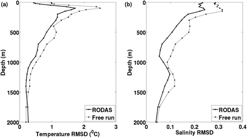
In the subsurface salinity, the assimilation run RMSD was reduced in the whole profile compared to the free run. The mean RMSD was 0.18 and 0.13 in the free run and in the RODAS run, respectively. The biggest impact was at 150 m, where the RMSD reduction corresponded to 29%, from 0.32 to 0.22. As mentioned above, models have difficulties in reproducing sharp gradients and this is also associated with the halocline. Since there is no assimilation of sea surface salinity, there is a high analysis error at the surface and down to 150 m, where it oscillates between 0.22 and 0.24. The free run RMSD oscillates between 0.28 and 0.32 at the same depth range. Below that, the RMSD gradually decreases in both experiments down to 900 m depth, where the RODAS run reaches 0.05 and the free run reaches 0.10. RODAS run surface salinity might decrease even more if SSS from satellite missions are assimilated. Overall, data assimilation effectively constrains the model towards observation and it has been demonstrated that HYCOM + RODAS has a relatively good skill in reproducing the ocean thermohaline state.

Assessment of the extended-range predictive skill

To provide an estimate of the decrease of the HYCOM + RODAS extended forecast skill, Figure 3 shows the RMSD and correlation of SST and SLA averaged over all 48 30-day hindcasts with respect to the RODAS run over Metarea V. It also shows the skill of persistence and free run. For both SST and SLA, the model hindcast had the lowest RMSD and the highest correlation throughout the 30-day windows. The evolution of SST RMSD shows that the hindcast slowly degraded, while persistence did it much more quickly, reaching the free run values by the 22nd day. By the 30th day, the persistence error reached 1.09°C, while the hindcast RMSD was 0.46°C. The free run error was almost constant with an average of 0.88°C. The SST correlation ranged from 1 to 0.94 for the hindcast and from 1 to 0.75 for persistence, which took 11 days to reach free run values. The latter had an average correlation of 0.89.

Figure 3. RMSD and correlation of SST and SLA with respect to RODAS analyses over 48 30-day cycles averaged over Metarea V. Black solid line represents the hindcast, the line with square markers represents persistence and the line with asterisk markers represents the free run.

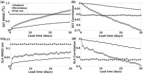
Considering SLA, the sharpest RMSD increase was in the first 24 h, when the hindcast value reached 0.02 m and the persistence error reached 0.05 m. Thereafter, the RMSDs increased at a similar rate, reaching 0.05 m in the hindcast and 0.08 m in persistence by the 30th day. The free run had the highest RMSD at all lead times, with an average of 0.13 m. The hindcast SLA correlation was consistently higher than persistence correlation, ranging from 1 to 0.79, while the latter ranged from 1 to 0.41. The free run correlation was always lower than 0.6. In general, the SLA errors grow more quickly than the SST errors. Although different assimilation systems and ocean models might have very different results, previous studies have had similar results, such as in Oke et al. (2015), where observations were withheld from the forecast system to provide an estimate of the decrease in analysis and forecast skill.

Since the hindcast was better than persistence at all lead times, the results suggest that the model adds some skill to the initialised state over a 30-day forecast. Also, the errors of the SST and SLA hindcasts are smaller than the errors of the free run. As expected, it demonstrates the benefit of data assimilation on the forecast skill and shows that an accurate initial condition considerably enhances predictability. Moreover, it gives an indication of the system tolerance to observation dropouts, as the hindcast error takes more than a month to saturate and reach the free run values. However, it must not be forgotten that the model was forced by atmospheric reanalysis fields. Therefore, it is not expected that the quality of these fields degrade over each forecast cycle as they would if the atmospheric forcing were a true weather forecast.

Figure 4 represents the evolution of the temperature and salinity RMSD in the subsurface for hindcast and persistence. The largest errors were in the upper ocean associated with both the mixed layer and the thermocline/halocline, and there is a gradual decrease in errors with depth, in line with a decrease in variability in the deeper ocean. This behaviour is in accordance with Divakaran et al. (2015). At 10 m depth, persistence had the highest temperature RMSD values and reached 0.76°C in day 30, when the hindcast RMSD reached 0.16°C. As observed in previous studies, in shallow waters and in the surface mixed layer, the ocean state is very sensitive to atmospheric forcing, rather than to the initial condition, therefore persistence quickly loses skill (Hurlburt et al. 2009; Martin 2011; Zhu 2011). At 100 m depth, the hindcast had the largest errors, reaching 0.19°C in day 28. This is associated with the thermocline and is in accordance with what was shown in Figure 2. Persistence took 17 days to reach the same RMSD value at this depth, indicating a positive hindcast skill even in the thermocline. In the deep ocean, the temperature RMSD decreased very slowly in both experiments. In 1000 m depth, persistence RMSD took 8 days to reach 0.01°C and the hindcast took 13 days to reach the same value (not shown). As described by Hurlburt et al. (2009), the deep ocean variability is non-deterministic with respect to atmospheric forcing, and the time scale for predictive skill depends mostly on the quality of the initial state, the accuracy of the model dynamics and the flow instability. In this region, the flow is dominated by the termohaline circulation, which evolves on longer time scales. The free run kept the RMSD values almost constant throughout the 30 days, with the highest values (1.81°C) near the thermocline. At all depths the free run error was higher than those of the hindcast, with an average of 0.63°C at 10 m depth and 0.25°C at 1000 m depth (not shown). Thus, HYCOM + RODAS skill in predicting temperature is not restricted to the surface, but extends to the deep ocean as well.

Figure 4. RMSD of the subsurface temperature (°C) [(a) and (b)] and salinity [(c) and (d)] with respect to RODAS over 48 30-day cycles averaged in Metarea V.

Similarly to temperature, the highest persistence salinity RMSD was near the surface, where the values reached 0.06 in 30-day lead time. In the hindcast, the error was not higher than 0.01 in any lead time at the surface. Near the halocline, hindcast produced the largest error, which is also in agreement with Figure 2. It reached 0.02 in the 26th day and persistence reached the same value in the 17th day. Below this depth, the error was fairly small in both experiments. At 500 m depth, both hindcast and persistence RMSD took 16 days to reach 0.01. In the free run, salinity RMSD was almost constant through time, but varied with depth, ranging from 0.01 at 5000 m to 0.11 at 300 m (not shown). These are reasonable results as salinity is a tracer quantity, which evolves on longer timescales than temperature in large parts of the ocean (Ryan et al. 2015).

Case study – an upwelling event on the southeast coast of Brazil

For a more detailed and qualitative assessment of HYCOM + RODAS predictive skill, a coastal upwelling event that occurred on 23 February 2011 on the southeast coast of Brazil was investigated (Figure 5). This feature evolves in the scale of days and it can be identified by a sharp SST gradient near the coast, due to the intrusion of slope water on the continental shelf (Aguiar et al. 2014). Figure 5 shows the SST fields from OSTIA, free run and two hindcasts, one initialised on 15 February 2011 and the other on 31 January 2011, corresponding to 8-day and 23-day lead time, respectively. Generally, the modelled SST fields compare well with the observation as they all capture a conspicuous surface signal of the event. This was expected, since coastal upwelling is primarily induced by wind-driven mechanisms (Aguiar et al. 2014), and the model representation of these events is strongly dependent on atmospheric forcing. However, free run shows an event with larger horizontal dimension than OSTIA, while in the hindcasts, the shape of the plume is more constrained towards observation. Furthermore, both hindcasts present an offshore stretched cold water filament at 40°W, which indicates a cyclonic circulation pattern. In AVISO SLA field, a cyclonic eddy is present at the same location (Figure 5(e)). The hindcasts were able to capture a signal of this feature, in both SST and SLA fields, while free run did not capture it at all. It is well established in the literature that coastal and oceanic systems do interact and the presence of cyclonic meanders/eddies can cause or enhance coastal upwelling (Campos et al. 2000; Calado et al. 2010; Aguiar et al. 2014). Therefore, the impact of the initial condition on the quality of the forecast is clear. It is also of note the clear warm bias the model develops, since the model SST in the 23-day lead time between 36° and 39°W is higher than in the 8-day lead time and the model free run is much higher than both hindcasts and observations.

Figure 5. SST (°C) [(a) to (d)] and SLA (m) [(e) to (h)] fields during an upwelling event on 23 February 2011. The solid black line represents the position of the vertical section. The black dashed lines represent the 100 and 1000 m isobaths.

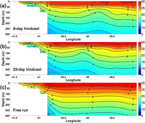
In the subsurface, the model simulations show slope water intrusions in the continental shelf, which is also an indication of upwelling (Figure 6). Both hindcasts were very similar, with 16°C temperatures observed at 50 m depth and the cyclonic eddy was evident from the uplift of the isotherms near 40°W, matching the position in AVISO SLA field (Figure 5(e)). In the free run section, the 16°C isotherm is only raised to 150 m depth and it did not capture the cyclonic eddy. Moreover, in the free run the mixed layer depth is deeper and the thermocline is much more diffuse than in the hindcasts. It reinforces that the assimilation system consistently improves the termohaline state of the ocean and that the model is able to retain some skill for at least 23 days.

Figure 6. Vertical sections of temperature (°C) during an upwelling event on 23 February 2011. The location of the section is shown in Figure 5.

Conclusions

HYCOM + RODAS system was assessed and compared to free run over the Atlantic Ocean Metarea V in 2011 and 2012. The results showed that overall data assimilation had a positive impact in the representation of the ocean state, reducing the RMSD of SST with respect to observations by 48%, and increasing the overall SLA correlation by 65%. On the subsurface, the average RMSD of temperature and salinity was reduced by 29% and 28%, respectively. RODAS was able to better represent areas of high variability and the termohaline state of the ocean was improved.

The predictive skill of 30-day hindcasts initialised with RODAS analysis was evaluated and compared to persistence and free run. The results revealed that for SST and SLA, the model hindcast had the lowest RMSD and highest correlation throughout the 30 days. Persistence degraded much more quickly than the hindcast, with a RMSD increase of 1.09°C for SST and 0.08 m for SLA over 30 days, while the hindcast had an increase of 0.46°C and 0.05 m over the same period. This suggests that the model typically adds some skill to the initialised state over a 30-day forecast. The free run RMSD (correlation) was always higher (lower) than that of the hindcast, demonstrating that an accurate initial condition considerably enhances HYCOM + RODAS predictability and the hindcast error takes more than a month to saturate.

The subsurface temperature and salinity RMSD showed that in small depths persistence RMSD rapidly increased to 0.76°C and 0.06 over 30 days, while hindcast RMSD increased to 0.16°C and 0.01. In shallow waters and in the surface mixed layer, the ocean state is very sensitive to atmospheric forcing, therefore, persistence quickly loses skill. In the deep ocean, temperature and salinity errors were fairly low, reaching 0.01°C and 0.01 after 30 days in both simulations. In this region, the time scale for predictive skill depends mainly on the quality of the initial state, the accuracy of the model dynamics and the time scale of the flow instability.

For a qualitative assessment, an upwelling event on the southeast coast of Brazil was investigated. Free run was able to reproduce the coastal upwelling event at the surface, but not at the subsurface. In contrast, both 8- and 23-day hindcasts represented a well-developed event as a whole and captured a signal of a cyclonic eddy, which was in accordance with AVISO SLA field. It reinforces that the assimilation system consistently improved the termohaline state of the ocean.

Overall, we conclude that the HYCOM hindcast initialised with RODAS analysis typically provides a good estimate of the ocean state over a 30-day window. However, these simulations represent the lowest bound of the ocean model errors considering all possible atmospheric forcings. For a real predictability assessment, true weather forecasts should be employed instead of atmospheric reanalysis fields.

Acknowledgments

We gratefully acknowledge the support of GODAE OceanView, Prof. Jiang Zhu by the Institute of Atmospheric Physics, Chinese Academy of Science (IAP/CAS), and the Project PIE00005/2016 of the State of Bahia Foundation for Research Support (FAPESB) Infrastructure Call 003/2015.

Disclosure statement

No potential conflict of interest was reported by the authors.

Additional information

Funding

The first and fourth authors would like to thank the Brazilian Conselho Nacional de Desenvolvimento Científico e Tecnológico (CNPq) for the research scholarship (123082/2016-1) and infrastructure grant (446528/2014-5). This work was also supported by PETROBRAS and the Brazilian oil regulatory agency ANP (Agência Nacional de Petróleo, Gás Natural e Biocombustíveis), within the special participation research project Oceanographic Modeling and Observation Network (REMO).

References

- Aguiar AL, Cirano M, Pereira J, Marta-Almeida M. 2014. Upwelling processes along a western boundary current in the Abrolhos–Campos region of Brazil. Cont Shelf Res. 85:42–59. doi: 10.1016/j.csr.2014.04.013
- Bleck R. 2002. An oceanic general circulation model framed in hybrid isopycnic-Cartesian coordinates. Ocean Model. 4:55–88. doi: 10.1016/S1463-5003(01)00012-9
- Brasseur P. 2006. Ocean data assimilation using sequential methods based on the Kalman filter. In: Ocean weather forecast. Dordrecht, Netherlands: Springer; p. 271–316.
- Calado L, da Silveira ICA, Gangopadhyay A, de Castro BM. 2010. Eddy-induced upwelling off Cape São Tomé (22°S, Brazil). Cont Shelf Res. 30:1181–1188. doi: 10.1016/j.csr.2010.03.007
- Campos EJD, Velhote D, da Silveira ICA. 2000. Shelf break upwelling driven by Brazil current cyclonic meanders. Geophys Res Lett. 27:751–754. doi: 10.1029/1999GL010502
- Chassignet E, Hurlburt H, Metzger E, Smedstad O, Cummings J, Halliwell G, Bleck R, Baraille R, Wallcraft A, Lozano C, et al. 2009. US GODAE: global ocean prediction with the HYbrid coordinate ocean model (HYCOM). Oceanogr. 22:64–75. doi: 10.5670/oceanog.2009.39
- Chassignet EP, Hurlburt HE, Smedstad OM, Halliwell GR, Hogan PJ, Wallcraft AJ, Baraille R, Bleck R. 2007. The HYCOM (HYbrid coordinate ocean model) data assimilative system. J Mar Sys. 65:60–83. doi: 10.1016/j.jmarsys.2005.09.016
- Costa F, Tanajura C. 2015. Assimilation of sea-level anomalies and Argo data into HYCOM and its impact on the 24 h forecasts in the western tropical and South Atlantic. J Oper Oceanogr. 8:52–62.
- Divakaran P, Brassington G, Ryan A, Regnier C, Spindler T, Mehra A, Hernandez F, Smith G, Liu Y, Davidson F. 2015. GODAE OceanView inter-comparison for the Australian region. J Oper Oceanogr. 8:s112–s126.
- Dombrowsky E. 2011. Overview of global operational oceanography systems. In: Schiller A, Brassington GB, editors. Operational oceanography in the 21st century. Dordrecht: Springer; p. 397–411.
- Evensen G. 2003. The ensemble Kalman filter: theoretical formulation and practical implementation. Ocean Dyn. 53:343–367. doi: 10.1007/s10236-003-0036-9
- Hernandez F, Blockley E, Brassington G, Davidson F, Divakaran P, Drévillon M, Ishizaki S, Garcia-Sotillo M, Hogan P, Lagemaa P, et al. 2015. Recent progress in performance evaluations and near real-time assessment of operational ocean products. J Oper Oceanogr. 8:s221–s238.
- Hurlburt H, Brassington G, Drillet Y, Kamachi M, Benkiran M, Bourdallé-Badie R, Chassignet E, Jacobs G, Galloudec O, Lellouche J, et al. 2009. High-resolution global and basin-scale ocean analyses and forecasts. Oceanogr. 22:110–127. doi: 10.5670/oceanog.2009.70
- Lima J, Martins R, Tanajura C, Paiva A, Cirano M, Campos E, Soares I, França G, Obino R, Alvarenga J. 2013. Design and implementation of the oceanographic modeling and observation network (REMO) for operational oceanography and ocean forecasting. Rev Bras de Geofis. 31:209–228.
- Martin M. 2011. Ocean forecasting systems: product evaluation and skill. In: Schiller A, Brassington GB, editors. Operational oceanography in the 21st century. Dordrecht, Netherlands: Springer Science+Business Media B. V.; p. 611–631.
- Mignac D, Tanajura CAS, Santana AN, Lima LN, Xie J. 2015. Argo data assimilation into HYCOM with an EnOI method in the Atlantic Ocean. Ocean Sci. 11:195–213. doi: 10.5194/os-11-195-2015
- Oke P, Larnicol G, Fujii Y, Smith G, Lea D, Guinehut S, Remy E, Balmaseda M, Rykova T, Surcel-Colan D, et al. 2015. Assessing the impact of observations on ocean forecasts and reanalyses: part 1, global studies. J Oper Oceanogr. 8:s49–s62.
- Ryan A, Regnier C, Divakaran P, Spindler T, Mehra A, Smith G, Davidson F, Hernandez F, Maksymczuk J, Liu Y. 2015. GODAE OceanView Class 4 forecast verification framework: global ocean inter-comparison. J Oper Oceanogr. 8:s98–s111.
- Tanajura C, Santana A, Mignac D, Lima L, Belyaev K, Ji-Ping X. 2014. The REMO ocean data assimilation system into HYCOM (RODAS_H): general description and preliminary results. Atmos Oceanic Sci Lett. 7:464–470. doi: 10.1080/16742834.2014.11447208
- Volkov DL, Larnicol G, Dorandeu J. 2007. Improving the quality of satellite altimetry data over continental shelves. J Geophys Res. 112:1–20.
- Xie J, Zhu J. 2010. Ensemble optimal interpolation schemes for assimilating Argo profiles into a hybrid coordinate ocean model. Ocean Model. 33:283–298. doi: 10.1016/j.ocemod.2010.03.002
- Zhu J. 2011. Overview of regional and coastal systems. In: Schiller A, Brassington GB, editors. Operational oceanography in the 21st century. Dordrecht, Netherlands: Springer Science+Business Media B. V.; p. 413–439.