Underwater noise levels in Indian waters off the coast of Mormugao Port

ABSTRACT

Among various factors influencing the ocean noise levels, shipping traffic radiated underwater noise levels were identified as the major contributors. The increase in ambient noise levels due to natural and anthropogenic sources threatens the marine species communication. India has a coastline of 7,516.6 Km with 12 major and ∼187 minor ports. The hydrophone system measured for 39 days helped in investigating the distant shipping traffic lane noise levels and its influence on ambient noise levels of the region. The ocean noise levels measurement were ∼115 dB re 1 µPa for the prevailing environmental conditions. The noise exposure levels were ∼10 dB higher at <1 kHz due to ship passage to and from the port. The fish noise dominated the ambient sea noise mostly at high frequencies >1 kHz. The maximum and minimum range of shipping noise spectra for both the month’s data indicated peak sound pressure level in the lower frequency. Thus, the outcome of the measurements helped in understanding ocean noise levels off the coast of Mormugao Port and the influence of shipping traffic. A similar study for longer duration shall be useful to develop specific traffic lanes in the port entrance which is free from the mammal movements.

KEYWORDS:

• Ambient noise
• shipping traffic lane
• fish noise and lower frequency

1. Introduction

For the past decade, a concern was raised that a significant portion of the underwater noise generated by human activity may be related to commercial shipping and other sources in the sea (Gassmann et al. 2017) and also recognised to have negative consequences on marine life, especially marine mammals of the region (Merchant et al. 2014; Putland et al. 2018). The acoustic data of a region has always been an important measure to understand the oceans. Underwater ambient noise is continuously generated by wind, waves and other sources in the sea. The coastal waters of India such as in the continental shelves, wind speed appears to determine the noise levels over a wide frequency range (Ramji et al. 2007). Ambient noise measurements along the Indian continental shelf helped in establishing seabed characteristics such as directionality and reflection coefficient, where noise directionality was temporally varying but reflection coefficient is the same for a particular site (Sanjana et al. 2013).

The present purpose of the study is to explore the influence of the shipping radiated noise levels on the ambient noise levels (Mckenna et al. 2012; Merchant et al. 2016; IQOE 2018) and coast of Mormugao Port is an important habitat of several marine mammals’ species (Parson 2006; Jamalabad and Bopardikar 2017). Similar studies on ambient noise levels in the east and west coast of Indian water were carried out with the aim to analyse the influence of rain and wind, which being the abiotic sources (Ashokan et al. 2015). However, this the first study of ambient noise measurements off the coast of Mormugao Port to analyse the shipping traffic influence. The shipping radiated noise levels are mainly due to the onboard machinery, flow around the hull and propeller cavitation, mostly in the low-frequency range <500 Hz (Pricop et al. 2010; MEPC circular 833 2014). Long-term acoustic measurements of the region shall be useful to establish the background noise levels and also for any future investigation to study mammals behaviour responses (Ellison et al. 2012; Merchant et al. 2014). Similar studies also help to see the feasibility of the developed ISO 17208 & other standards for measurements of underwater noise radiated by the ships in Indian waters. It shall also help the ship designer, shipbuilders and ship operators for effective reduction in the ship radiated noise and improve the ship safety and energy efficiency (25th International Towing Tank Conference 2008).

Anthropogenic noise may threatens the ability of vocalising marine species to communicate, which vocalise at low frequency in particular region, mostly close to vessel traffic movement (Putland et al. 2018). The marine mammal's species mainly foraging in the present location of study, where deliberated by researchers in multiple occasions and also sighted many mammals presence in a habitat like humpback dolphins (Sousa chinensis), finless porpoises (Neophocaena phocaenoides), Killer whales (Orcinus orca) and a humpback whales (Megaptera novaeangliae) (Parson 2006; Jamalabad and Bopardikar 2017). Indian humpback dolphins groups where mostly found in the coastline, clusters foraging near river mouths towards the Goa port. The acoustic measured data of communication frequencies of Indian humpback dolphins in the present location is inadequate. But, similar work for the same species is available for west Hong Kong region with whistle and barks disturbance recordings mostly concentrated in the mid-frequency range (Sims et al. 2012). The threshold of hearing of one sound if raised by the presence of another sound masking occurs (Erbe et al. 2015). This may vary with many parameters based on the type of species, ocean condition, distance between source and receiver, depth of the receiver etc.

The study mainly focused to bridge the knowledge gap on the influence of shipping traffic noise to and from the Mormugao Port on the ambient noise levels and establishing the baseline levels which will be useful for future noise monitoring studies. The measured noise data if combined with the ship’s Automatic Identification System (AIS) data shall be useful to establish the ship radiated noise based on ship type, size, propeller rpm and also help in developing soundscapes due to ship movement in the region at different depths (Merchant et al. 2012; Putland et al. 2018). Moreover, the underwater noise levels due to shipping traffic is viewed to mask the marine mammal’s low frequency vocalisation with severe effects on their biological activities and also increase the ambient noise levels due to continuous vessel movement (Morisaka et al. 2005; Nowacek et al. 2007; Hatch et al. 2008).

2. Methods

2.1. Measurement system and deployment location

An autonomous system interfaced with data acquisition system for time series measurements of ocean noise levels was developed by National Institute of Ocean Technology (NIOT), Chennai, Ocean Acoustics and Modelling group. The group was involved in research and development in varied topics such as systems for acoustic applications. One of the research areas is to measure the ambient noise levels of Indian water with real-time communications (NIOT, n.d.). A vertical Omni-directional hydrophone calibrated at Acoustic Testing Facility of NIOT, with specifications as indicated in Table 1 Hydrophone Specifications was deployed in the region. The mean sensitivity measured is −162 [dB re 1 V/μPa] for frequencies 400–1100 Hz at 100 Hz interval. The sensor is encased in an oil filled polyurethane tube, deployed off the coast of Mormugao Port at latitude N15d 21.526 m longitude E73d 3.854 m, which is ∼30 nautical miles from the coastline and ∼27 nautical miles from the port entrance. The hydrophone is deployed at depth of 11 m in a water depth of 22 m. Figure 1 shows the general view of the Indian map indicates the Goa regions. The normal shipping passage traffic lane is ∼18 nautical miles away from the hydrophone deployment site indicated in Figure 2. The data acquisition system and battery are encased in an enclosure and housed in the surface buoy along with data communication modules. Network noise stations setup for data collection has a recording and transmitting signal facility. The measured data is transmitted in total eight datasets per day say (1, 4, 7, 10 am, 1, 4, 7, 10 pm) with time interval gap of 3 h for the total period of 39 days as indicated in Table 2 Data collected period. The total datasets measured are 312 with 8 datasets per day. Because of the system limitation and AIS data restriction, the measured data could not be interrelated to the AIS data. However, all the datasets need to be processed to filter the ambient, anthropogenic and fish noise datasets using a post-processing methodology as discussed in Section 2.2.

Figure 1. Mormugao port general view on Indian map.

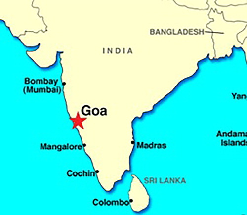
Figure 2. Hydrophone deployment location and Mormugao port ship traffic lane. Map obtained from Marine traffic.com website.

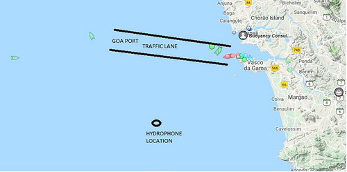
Table 1. Hydrophone specifications.

Make	Keltron
Model	KE10
Sampling frequency	25 kHz
Data duration	30 sec
Receiving sensitivity	−162 dB

Table 2. Data collected period.

Deployment location	Start date	End date	No. of days
Goa	17 May 2012	31 May 2012	15 days
Goa	04 June 2012	27 June 2012	24 days

2.2. Data processing

The autonomous underwater acoustic system recorded data that measured the sound signal as the changes in underwater sound pressure levels (SPL) re 1 µPa in an electrical voltage signal form by the hydrophone transducer. The voltage signal file is processed using MATLAB wave write script to a ‘.wav’ sound file format using hydrophone sample rate and NBITS (MATLAB, n.d.). The power spectral density was calculated using a Hanning window with 75% overlap for all the datasets obtained for 39 days using Spectra plus-SC, Fast Fourier Transformation spectral analysis programme used to post-process the time domain signal to the frequency domain.

An adaptive threshold level (ATL) method was used to identify the ship passage noise level over the background noise levels. The ATL works on the assumption that the minimum SPL over the window duration of all the datasets as the background noise level. Considering a fixed threshold limit of 6 dB over the established minimum SPL shall be identified as of the local shipping, anthropogenic and other noise sources (Merchant et al. 2012). The filtered datasets were later confirmed to be shipping noise or other noises by listening to the corresponding audio file.

3. Environmental conditions

Meteorological data required for the measured site was obtained from the Asia – Pacific Data Research Center open-access database (International Pacific Research Center at the University of Hawaii at Manoa 2008) from University of Hawaii. The dataset obtained from the models iCOADS 1 × 1 enhanced and DASK 1.4 for the location longitude 73.5 E, latitude 15.5 N, it included parameters in the nearest available region to the measured site as indicated in Table 3 Meteorological data. The datasets obtained on daily basis indicated a linear change in the parameters for the two months with no abnormal changes in the weather conditions.

Table 3. Meteorological data.

Dataset (Mean value)	May 2012	June 2012
Wind speed	7 m/s	7.5 m/s
Zonal wind speed	4.2 m/s	5.2 m/s
Sea Surf Temp	28.3 degc	27.9 degc
Sea level pressure	1008.40 mb	1007.40 mb
Salinity 5, 15 and 25 m depths	35.42 psu 35.42 psu 35.46 psu	35.30 psu 35.30 psu 35.38 psu
i current 5, 15 and 25 m depths (x-direction)	0.0165 m/s −0.0070 m/s −0.015 m/s	0.0161 m/s −0.0130 m/s −0.035 m/s
j current 5, 15 and 25 m depths (y-direction)	−0.0303 m/s −0.021 m/s 0.004 m/s	−0.0307 m/s −0.026 m/s −0.0045 m/s

4. Results

The hydrophone measured data was collected from the test site for 15 days in May 2012 and 24 days in June 2012. The data helped in establishing the acoustic signatures of anthropogenic or distant shipping sources and other marine life communication noise levels.

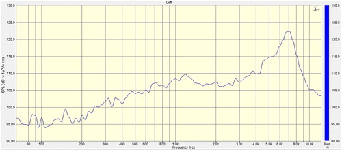
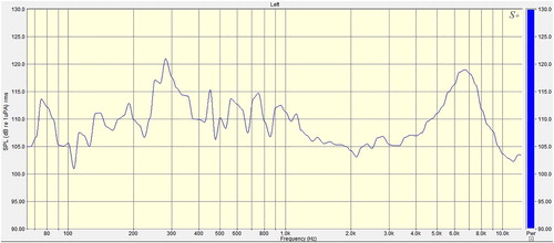
1. The underwater noise levels of the ocean are mostly attributable to wind, tidal process and the fauna of the region, these being sources of underwater ambient noise (Wenz 1962; Bardyshev 2007). The influence of rain and higher wind speeds are associated with broadband noise concentration in the higher frequency range (M Ashokan et al. 2015; Sudhir and Lohani 2016). In the present measurement, the mean peak ocean noise amplitudes are around 102 dB re 1 µPa at frequencies <4 kHz as shown in Figure 3. The maximum sound pressure levels are around 120 dB re 1 µPa at higher frequency ∼6 kHz. This is mainly due to other marine invertebrates sources say sea urchins, snapping shrimp with loud snap sound generated by popping of bubbles (Everest et al. 1947; Johnson et al. 1948; Au and Banks 1998).

Figure 3. Ocean noise levels spectrum indicating peak noise levels at 6.7 kHz.

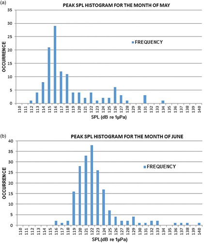
2. From all the datasets collected for the 39 days hydrophone data, the peak sound pressure levels (SPL) histogram indicated that the peak occurrences of SPL is ∼116 dB re 1 µPa for the month of May indicated in ‘A’ Figure 4 and ∼122 dB re 1 µPa for the month of June in ‘B’ Figure 4. This increase in the peak noise levels is due to natural as well as human contributions. This indicates a warning alarm on the increase in ambient levels of the region. However, a similar study for a longer period shall be useful to understand the changes in the ambient noise levels of a region.

Figure 4. The peak sound pressure levels (SPL) histograms indicating the noise levels occurrences in a month (A) May (B) June.

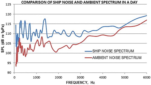
3. On comparison of frequency spectrums of the datasets with shipping noise and without shipping noise for the same day as shown in Figure 5, indicates an increase in daily noise exposure levels above the ambient noise levels by ∼10 dB for frequencies <1 kHz and ∼4 dB > 1 kHz due to ship passage. This indicates that the ship-radiated noise in oceans has influence in raising the ambient noise levels of ocean mostly in the low-frequency range due to ship passage.

Figure 5. Comparison of ship noise and ambient noise spectrums in the frequency range up to 6 kHz.

4. On analysing the ship noise data, it indicated dominant frequencies <500 Hz, with peak RMS noise levels ∼123 dB re 1 µPa at 300 Hz as shown in Figure 6 Ship noise 1/12 octave frequency spectrum from a dataset with 30-sec duration in a day. The peak noise levels in lower frequencies indicate the source frequencies mainly from the propeller, main engine, auxiliary engines, flow noise etc. (Pricop et al. 2010). The exact correlation can be only be made, if the ship details in operation are available from AIS.

Figure 6. Ship noise 1/12 octave frequency spectrum from a dataset with 30-sec duration in a day.

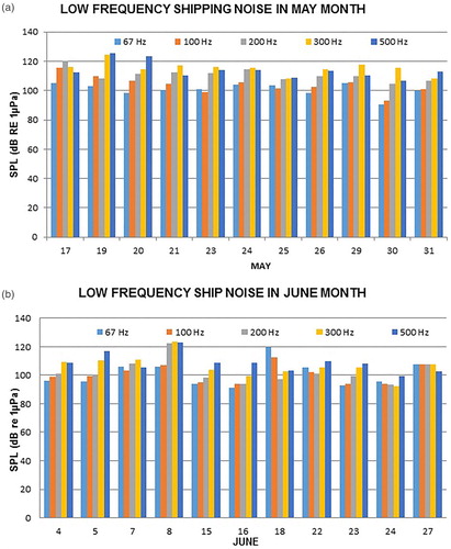
5. The shipping noise datasets of low-frequency noise levels at 67, 100, 200, 300, and 500 Hz, indicates a SPL range between 90–120 dB. The general trend indicates an increase in the noise levels from low to high frequency within the range <500 Hz as shown in Figure 7 Low-frequency day-wise shipping noise levels (A) May (B) June. ‘A’ for the month of May and ‘B’ for the month of June.

Figure 7. Low-frequency day-wise shipping noise levels (A) May (B) June.

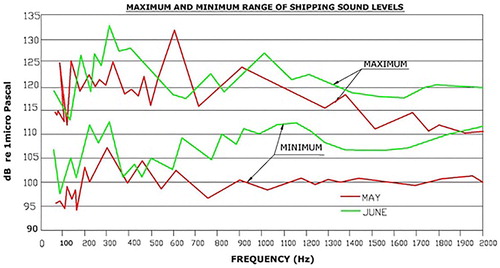
6. The sound levels of all the ship datasets indicate the maximum and minimum SPL in dB re 1 µPa for both May and June months. The maximum SPL is around 132 dB re 1 µPa and minimum SPL is around 95 dB re 1 µPa as shown on Figure 8 Range of sound levels of ship datasets for both May and June months. The maximum and minimum range of sound levels obtained by plotting the envelope of all the ship noise datasets. The variation in the spectra for both the months at different frequencies may be due to the ship type, operation condition and environmental parameters (McKenna et al. 2012; Merchant et al. 2012).

Figure 8. Range of sound levels of ship datasets for both May and June months.

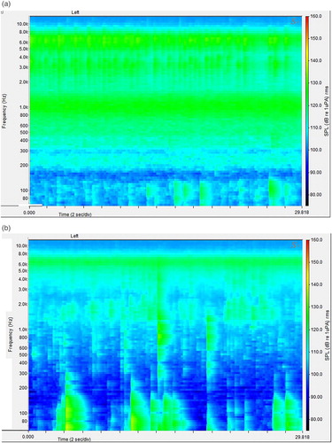
7. Some data also indicated some fish and other marine invertebrates (say snapping shrimp) noises which sound like ‘pop’ and ‘trumpet’. The chorus occurrence dominated the ambient sea noise spectra. The generated sound was higher during hours of dusk with a peak in noise levels ∼125 dB re 1 µPa around 1–2 kHz as shown in spectrogram (‘A’ in Figure 9) and the fish disturbance in the lower frequency are indicated in the spectrogram (‘B’ in Figure 9) (Sims et al. 2012; University of Rhode Island and Inner Space Center. 2017; Putland et al. 2018).

Figure 9. The Fish noise spectrogram indicating the disturbances in (A) High frequency (B) low frequency.

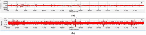
8. The spectrogram of the dataset indicated below show the disturbance created by distant shipping noise in the low-frequency region (‘B’ in Figure 10) as compared with the ambient conditions spectrogram (‘A’ in Figure 10). Figure 11 ‘C’ shows the time series signal of the ambient conditions for the same dataset and Figure 11 ‘D’ show the time series signal of the disturbance due to the ship passage.

Figure 10 . The Ocean noise spectrogram indicating the ambient and ship passage disturbance (A) Ambient on 19 May 2012 at 10:00 AM (B) Ship disturbance 19 May 2012 at 4:00 AM.

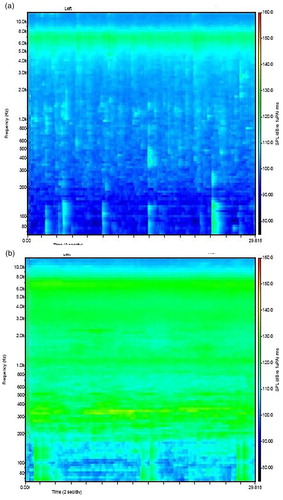
Figure 11. The time series representation of ocean noise levels for the 30-sec duration (C) Ambient 19th May 2012 at 10:00 AM (D). Ship disturbance 19 May 2012 at 4:00 AM.

5. Conclusion

The underwater noise levels off the coast of Mormugao Port are greatly influenced by the presence of noise from the shipping traffic to and from the Port. The present location is a habitat of different marine species like humpback dolphins, Orcas, Finless porpoises, fishes etc., sighted foraging in the region (Jamalabad and Bopardikar 2017). The increase in ambient noise may bring behavioural responses and increase chronic stress in the marine species (Ellison et al. 2012).

In the present study, the 39 days measured data for two months, when analysed helped to establish the baseline noise levels and by using an adaptive threshold limit method helped to identify the shipping and other noise sources. The ocean noise levels are around 105 dB re 1 µPa for frequency <4 kHz and with peak noise levels at 6.7 kHz due to loud snap sound generated by marine invertebrates Figure 3. The month of June observed a higher sound pressure levels around 122 dB re 1 µPa in comparison to the month of May being 116 dB re 1 µPa as indicated in Figure 4. The possible reason for the increase in sound pressure levels may be due to vessel passing near to the deployment system location and also environmental parameters.

The anthropogenic (shipping traffic) noise into the marine environment altered the background noise levels from their natural state. The ship noise became a dominant factor by raising the noise levels by over 10 dB re 1 µPa in the lower frequency range over the ambient levels Figure 5. The maximum and minimum range of the shipping noise datasets indicated a peak sound pressure levels in the lower frequencies Figure 8. Nevertheless, the difference in the sound pressure levels shall further get affected by any future increase in shipping noise in the region.

Most of the studies in the Indian waters are mainly limited to the research on the influence due to wind, rain and flow velocity parameters on ambient noise levels (Ramji et al. 2007; M. Ashokan et al. 2015). Clearly, indicating the knowledge gap in the area of acoustic impact studies on marine life. The measured noise levels also contained other biological sounds such as snapping shrimp and fish communication signals in the low and high frequencies Figure 9. The measured data has limited the study to understand the effects of auditory masking on aquatic mammals of the region.

The present study is first of its kind at the entrance of a port region in India, which helped to establish that the shipping traffic influence the increase in the baseline noise levels of the region. There is a need to develop techniques for long-term underwater noise measurements as a step to understand the changes in the acoustic environment and how it affects marine life. Our measured data had limitation to assess the ship-type based analysis with great clarity due to unavailability of AIS data. However, further work is required to establish a methodology that will aid understanding of the noise exposure levels in connection with AIS data, as has been done in other countries (e.g. Merchant et al. 2012). This will help to develop mitigation measures that are appropriate in Indian waters. These studies shall also help to improve ocean environment for safe habitat of marine fauna.

Acknowledgment

The data collected was provided from National Institute of Ocean Technology (NIOT), Chennai, Ocean Acoustics and Modeling group and Asia Pacific Data Research (APDRC). We thank them for sharing the data which helped in understanding and studying the noise levels of the region.

Disclosure statement

No potential conflict of interest was reported by the authors.

References

- 25th International Towing Tank Conference. 2008. Cavitation survey. The Japan Society of Naval Architects and Ocean Engineers. Fukuoka: ITTC; p. 473–5333.
- Ashokan M, Latha G, Ramesh R, Thirunavukkarasu A. 2015. Analysis of underwater rain noise from shallow water ambient nosie measurements in Indian seas. Journal of Geo-Marine Sciences. 44(2):144–149.
- Au WWL, Banks K. 1998. The acoustics of the snapping shrimp Synalpheus parneomeris in Kaneohe Bay. J Acoust Soc Am. 103(1):41–47. doi: 10.1121/1.423234
- Bardyshev VI. 2007. Underwater ambient noise in shallow-water areas of the Indian ocean within the tropical zone. Acoust Phys. 53:167–171. doi: 10.1134/S1063771007020091
- Ellison WT, Southall BL, Clark CW, Frankel AS. 2012. A new context-based approach to assess marine mammal behavioral responses to anthropogenic sounds. Conserv Biol. 26:21–28. doi: 10.1111/j.1523-1739.2011.01803.x
- Erbe C, Reichmuth C, Cunningham KC, Lucke K, Dooling RJ. 2015. Communication masking in marine mammals: a review and research strategy. Mar Pollut Bull. 103(1-2):15–38. doi: 10.1016/j.marpolbul.2015.12.007
- Everest FA, Johnson MW, Young RW. 1947. The role of snapping shrimp (Crangon and Synalpheus) in the production of underwater noise in the sea. Biol Bull. 93:122–138. doi: 10.2307/1538284
- Gassmann M, Wiggins SM, Hildebrand JA. 2017. Deep-water measurements of container ship radiated noise signatures and directionality. J Acoust Soc Am. 142:1563–1574. doi: 10.1121/1.5001063
- Hatch L, Clark C, Merrick R, Van Parijs S, Ponirakis D, Schwehr K, Thompson M, Wiley D. 2008. Characterizing the relative contributions of large vessels to total ocean noise fields: a case study using the Gerry E. Studds Stellwagen Bank National marine sanctuary. Environ Manag. 42:735–752. doi: 10.1007/s00267-008-9169-4
- International Pacific Research Center at the University of Hawaii at Manoa. 2008. ALL datasets. Asia-Pacific Data Research Center. http://apdrc.soest.hawaii.edu/.
- IQOE. 2018. International quiet ocean experiment. Scientific Committee on Oceanic Research (SCOR) and the Partnership for Observation of the Global Oceans. https://www.iqoe.org/.
- Jamalabad A, Bopardikar I. 2017. Conservation India. http://www.conservationindia.org/wp-content/files_mf/Goa-MPT2.pdf.
- Johnson MW, Young RW, Everest FA. 1948. Acoustical characteristics of noise produced by snapping shrimp. J Acoust Soc Am. 137. doi: 10.1121/1.1906355
- McKenna MF, Ross D, Wiggins SM, Hildebrand JA. 2012. Underwater radiated noise from modern commercial ships. J Acoust Soc Am. 131:92–103. doi: 10.1121/1.3664100
- MEPC1 circular 833. 2014. IMO marine environmental protection committee. IMODOCS. https://docs.imo.org/Category.aspx?cid=108.
- Merchant ND, Brookes KL, Faulkner RC, Bicknell AWJ, Godley BJ, Witt MJ. 2016. Underwater noise levels in UK waters. London: Springer Nature scientific reports.
- Merchant ND, Pirotta E, Barton TR, Thompson PM. 2014. Monitoring ship noise to assess the impact of coastal developments on marine mammals. Mar Pollut Bull. 78:85–95. doi: 10.1016/j.marpolbul.2013.10.058
- Merchant ND, Witt MJ, Blondel P, Godley BJ, Smith GH. 2012. Assessing sound exposure from shipping in coastal waters using a single hydrophone and automatic identification system (AIS) data. Mar Pollut Bull. 64:1320–1329. doi: 10.1016/j.marpolbul.2012.05.004
- Morisaka T, Shinohara M, Nakahara F, Akamatsu T. 2005. Effects of ambient noise on the whistles of Indo-Pacific bottlenose dolphin populations. J Mammal. 86:541–546. doi: 10.1644/1545-1542(2005)86[541:EOANOT]2.0.CO;2
- Nowacek DP, Thorne LH, Johnston DW, Tyack PL. 2007. Responses of cetaceans to anthropogenic noise. Mammal Rev. 37:81–115. doi: 10.1111/j.1365-2907.2007.00104.x
- Parson ECM. 2006. Observations of Indo-Pacific humpbacked dolphins, Sousa chinensis, from Goa, Western India. Mar Mamm Sci. 14(1):166–170. doi: 10.1111/j.1748-7692.1998.tb00702.x
- Pricop M, Chitac V, Florin G, Pazara T, Oncica V, Atodiresei D. 2010. Underwater radiated noise of ships machinery in shallow water. In: 2nd International conference on manufacturing Engineering Quality and Production system. Research Gate. p. 71–76.
- Putland RL, Merchant ND, Farcas A, Radford CA. 2018. Vessel noise cuts down communication space for vocalizing fish and marine mammals. Glob Chang Biol. 24:1708–1721.
- Ramji S, Latha G, Ramakrishnana S. 2007. Analysis of fluctuations in wind dependent shallow water ambient noise spectrum. Fluct Noise Lett. 7(3):L313–L319. doi: 10.1142/S0219477507003969
- Sanjana MC, Latha G, Mahanty MM. 2013. Seabed characteristics from ambient noise at three shallow water sites in Northern Indian ocean. J Acoust Soc Am. 134(4):EL366–EL372. doi: 10.1121/1.4818936
- Sims PQ, Vaughn R, Hung SK, Würsig B. 2012. Sounds of Indo-Pacific humpback dolphins (Sousa chinensis) in west Hong Kong: A preliminary description. J Acoust Soc Am. 131:EL48–EL53. doi: 10.1121/1.3663281
- Sudhir PSR, Lohani RD. 2016. Ambient noise analysis and modeling in shallow water of Arabian Sea. Int J Comput Appl. 142(5):1–3.
- University of Rhode Island and Inner Space Center. 2017. Discovery of sound in the Sea. Dosits: https://dosits.org/.
- Wenz GM. 1962. Acoustic ambient noise in the ocean: spectra and sources. J Acoust Soc Am. 34:1936–1956. doi: 10.1121/1.1909155