Tracking fishing ground parameters in cloudy region using ocean colour and satellite-derived surface flow estimates: A study in the Bay of Bengal

ABSTRACT

A new conceptual framework, based on ocean bio-physical observations from different satellites, has been proposed to track fishing ground parameters to identify Potential Fishing Zones (PFZ) in the Bay of Bengal (BoB). The proposed technique also attempts to provide a short-term forecast based on feature propagation, even under cloudy conditions. The current study has been carried out to understand the link between possible fish catch availability and satellite-derived parameters such as chlorophyll concentration, sea surface temperature, sea-level anomaly, ocean surface currents and wind vectors. Net Ekman transport obtained from the upfront and downfront components of the wind relative to the frontal direction provides valuable information on the forecast of PFZ regions and its possible shift. Comparison of the identified PFZs with limited in situ fish catch data proves that the suggested approach holds the promise in improved monitoring of possible fish catch locations. The study provides a novel approach for the monitoring and short-term forecasting of PFZ even for cloud-contaminated regions by using all possible ocean information from space-based platforms.

KEYWORDS:

• PFZ
• oceanic eddy
• thermal front
• chlorophyll concentration
• upfront/downfront winds

1. Introduction

For fishing industry, at the basic production level, the availability of fishable concentrations of fishes and other marine life is a decisive factor, which controls the economy of fishing operations (Pillai and Abdussamad 2008). Even when well-equipped vessels, fishing gear and experienced fisher are available, the successes of fishing operation are dependent on the availability of fishable concentrations of commercially important marine life in space and time. The behaviour of fish habitats is controlled by variations observed on important environmental parameters such as seawater temperature, salinity, dissolved oxygen concentrations, currents, the presence of phytoplankton, zooplankton, etc. (Mittelbach et al. 2014). The absence of knowledge about the availability of fishes, their schools and shoals can result in waste of valuable time, effort and fuel. In India, with a coastline of more than 7500 km and exclusive economic zone (EEZ) of about 2 million square km, the potential yield of seafood is estimated to be around 3.9 Mt (Sankari 1996). Hence, it is essential to have the potential fishing zone (PFZ) identification, mapping, forecasting and validation on operational basis over the Indian EEZ water by tracking physical and biological parameters.

Satellite-derived chlorophyll concentrations (CHL) and sea surface temperature (SST) have been traditionally used widely across the world for the identification and mapping of PFZ. Oceanic fronts are the boundary between water masses of different physical and chemical properties and these are marked by narrow zones of enhanced temperature, salinity and biological gradients. Ocean thermal fronts are well known for upwelling and high chlorophyll contents (Owen 1981; Reese et al. 2011). Elevated chlorophyll structures associated with fronts are reported for the study area, Bay of Bengal (BoB) (Wijesekera et al. 2016) and high concentrations of chlorophyll are mostly associated with cool waters (low SST), mainly induced from upwelling (Abbott and Zion 1985; Chavez et al. 1999) and they are the indicators of the fish populations (Sissenwine 1984; Carpenter et al. 1985). Fishes are known to respond well with changes in temperature and they congregate around the upwelling boundaries of cold deep waters rich of phytoplankton (Choudhury et al. 2007; Belkin et al. 2009).

Many previous studies have used surface chlorophyll from Ocean Colour Monitor (OCM), SeaWiFS, Coastal Zone Color Scanner (CZCS), etc. and SST from AVHRR (Laurs 1993; Solanki et al. 2001; Solanki et al. 2003; Solanki et al. 2005) extensively to demonstrate the efficient forecast of PFZ. Such satellite remote sensing methods have been adopted by many countries such as India (Nayak et al. 2003; George et al. 2013), China (Mansor et al. 2001), Japan (Yamanaka 1988) etc. to monitor PFZ and to aid fishing folk community. As far as India is concerned, PFZ forecasting plays a significant role for the cost-effective fish catch along its coastal states such as Gujarat coast (Solanki et al. 2001; Nayak et al. 2003; Solanki et al. 2003; Dwivedi et al. 2005), Andaman Nicobar (George et al. 2013), Kerala coast (Pillai and Abdussamad 2008), Odisha coast (Sahu et al. 2012), Mumbai coast (Kamei et al. 2014) etc. Proper utilisation of these ocean features, e.g. thermal front (Nayak et al. 2003; Solanki et al. 2003; Ardianto et al. 2017) and CHL forms the basis for the efficient monitoring of PFZ. Continuous availability of satellite-based high-resolution SST and CHL is a major challenge, especially in the BoB, which is cloudy almost throughout the year (Zuidema 2003). Hence it becomes essential to explore additional parameters from satellite and identify some features which may be useful in the PFZ identification/monitoring. For e.g., mesoscale eddies have a significant role in modulating the distribution of CHL and nutrient cycling in the ocean (Mahadevan 2014; Singh et al. 2015). Other ocean parameters, such as location and evolution of frontal boundaries, upwelling zones, currents, eddies, etc., are important in defining marine fish habitats (Balaguru et al. 2014).

Wind-driven Ekman transport associated with fronts play a crucial role in re-stratifying the frontal features (Wickett 1967) and the frontal features can be reinforced by convective mixing induced by the cross-front Ekman transport forced by down-front wind (Mahadevan 2016). The hypothesis of our study is that by linking these additional features with conventional method based on thermal gradients and chlorophyll fronts will lead to better PFZ identification. With the addition of Ekman transport obtained from relative wind (difference between scatterometer wind and ocean surface currents) and accounting for upfront/downfront transport, it is expected to improve the scope of PFZ identification and forecast (Thomas 2005; Thomas and Lee 2005).

In the present study, a new approach has been developed to aid fishery industry by linking the essential ocean information available from various satellites, such as ocean colour, altimeter, scatterometer and radiometer with marine fishery potential zones. This is done by tracking important fishing ground parameters such as eddies from sea surface height (SSH), thermal fronts from SST, winds, ocean surface currents and CHL using the proposed methodology. The novel part of the methodology lies in the short-range PFZ prediction under cloudy conditions, by synergistically using information of thermal fronts, Ekman transport and ocean surface currents.

2. Study area, data used and methodology

The study area is BoB, where the proposed methodology for monitoring and forecasting of PFZ has been demonstrated. BoB is an area of high biodiversity and the coastal stretch having many fish landings which contribute more than 7% of the world’s catch (Naylor et al. 2000; Islam 2003). BoB is a unique basin as it receives lot of fresh water from Ganges, Brahmaputra and other rivers during southwest monsoon season. The upper layer stratification caused by the fresh water creates the barrier layer and warms the upper ocean, making it a biologically not so productive basin. BoB is home to many cyclonic and anticyclonic eddies. We briefly describe general oceanographic characteristics of this important basin.

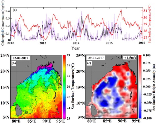
The mean ocean circulation and associated oceanic conditions of the study region are the result of the unique wind patterns associated with Indian Ocean monsoon (Schott and McCreary Jr 2001; Shankar et al. 2002). During summer monsoon, wind blows from south-west and impacts the biodiversity of BoB mainly through the wind-driven upwelling (Sharma 1978; Field et al. 1998; Kahru et al. 2010). The cool and nutrient-rich upwelled waters promote the growth of phytoplankton in BoB; this can be observed in Figure 1(a), depicting low SST and high CHL. High precipitation and river discharge associated with summer monsoon have deep and unique impact on the oceanic conditions of BoB, especially during post monsoon period. A strong barrier layer forms in BoB (Rao and Sivakumar 2003) as a result of intense freshening of surface layers during this period which obstructs the vertical mixing. As the link with subsurface is almost vanished during this period, modulations/disturbances happen at surface get intensified such as winter surface cooling. Another ubiquitous feature of BoB is the mesoscale eddies, which play an important role in the distribution of chlorophyll (Falkowski et al. 1991; Frenger et al. 2018). Figure 1(c) shows the variability of Sea Level Anomaly (SLA) during the winter period (December–February 2016). Chlorophyll patterns associated with the eddies depend on the vorticity of the eddies, which defines them as cyclonic and anti-cyclonic eddies. Cyclonic eddies are cold core eddies and promote the growth of phytoplankton at the eddy centre through positive vertical velocity, which brings more nutrients and subsurface chlorophyll to the surface. A typical distribution of SST and thermal fronts is shown in Figure 1(b) for 2 February 2017, representative of winter month. SST in the north BoB is less as compared to south BoB, clearly exhibiting the impact of cold north-east winter winds. One can clearly see dense frontal features in the North Bay of Bengal. Southern BoB is devoid of such features. Many of these fronts are aligned along the coast, which are extremely useful in identifying PFZ locations.

Figure 1. (a) Three-day running time series (2012–2016) of (left axis) CHL (mg/m³) and (right axis) SST(^oC) averaged over the study region (b) Snapshot of SST (^oC) overlaid with frontal lines (black lines) on 2 February 2017 and, (c) Weekly averaged (centred on 29 January 2017) sea-level anomaly (m) overlaid with ISRO-current.

2.1. Dataset used

Various oceanic and atmospheric parameters from different satellites are processed for understanding the relation between fish catch locations and ocean parameters. Chlorophyll products, (CHL of 4 km resolution daily data) from Globcolour-merged products data archive (European Space Agency, ESA), have been used (http://hermes.acri.fr/). To reduce the cloud coverage, the daily data have been averaged for 3 days and composites have been generated. SST used in this study is a 1 km L4-gridded GHRSST product taken from Global Data Archiving Centre (GDAC) of NASA JPL (http://podaac.jpl.nasa.gov/). Excellent quality observations of ocean surface wind vectors available from ISRO launched scatterometer, SCATSAT-1 is also being used in the study (www.mosdac.gov.in). OSCAR current data of 25 km resolution generated by SAC, ISRO (Sikhakolli et al. 2013), (www.mosdac.gov.in) have been analysed along with SCATSAT −1 scatterometer data to generate relative wind field vectors. Upwelling index computed using SCATSAT-1 winds are used to mark upwelling zones and are obtained from www.mosdac.gov.in. SSH anomaly from merged and gridded satellite product of Absolute Dynamic Topography produced and distributed by AVISO (http://www.aviso.oceanobs.com/) has been used to detect cyclonic (cold core) and anticyclonic (warm core) eddies. This product consists of maps of 7-day intervals on a 0.25^o spatial resolution. The total fish catch data have been received from Fishery Survey of India (FSI) for BoB waters to validate the method. Datasets obtained for the year 2016 have been used to demonstrate the proposed algorithm for the tracking of fishing ground parameters and an independent validation of the algorithm has been done using the data for January–March 2017.

2.2. Methodology for PFZ monitoring and forecasting

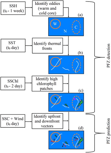
This section explains the major steps adopted to track fishing ground parameters to develop a feature-based PFZ monitoring and prediction system. PFZ algorithm proposed in the study has two parts, namely detection and prediction for the next few days. The first part is the detection/monitoring of PFZ using the information from fishing ground parameters such as eddy, thermal fronts, CHL and upwelling. The second part involves the prediction or tracking of the detected PFZ using information from thermal fronts, down-front and up-front components of relative wind fields and ocean surface current. Different steps in the algorithm have been detailed in the following sections and are shown in Figure 2.

Figure 2. Potential fishing zone identification: A comprehensive schematic from satellite-based multi-sensor observations. Thermal fronts, eddies and chlorophyll concentration patches are shown as white lines, dashed and contineous circles and lightening bolt symbol, respectively. W: Warm core Eddy, C: Cold core Eddy, N: No eddies. different color vectors represent Ekman transport and frontal direction. * in (c) represents the preferable ocean conditions for identifying PFZ.

2.2.1. The detection/monitoring of PFZ using fishing ground parameters

The first part of the methodology involves the identification and tracking of the eddies and the thermal fronts. The eddy location, type and intensity have a key role in the growth of fish schools. For eddy detection, we use a combination of techniques from Chelton et al. (2011) and Mason et al. (2014) that are suitably modified for robust identification and tracking of the BoB eddies. The original algorithms from Chelton et al. (2011) and Mason et al. (2014) were experimented to identify suitable eddy amplitude and size thresholds in order to reduce false alarms for the BoB region. After several experiments, the final threshold of size and amplitude was fixed as 400 km and 5 cm, respectively. To identify the mesoscale eddy features, only the mesoscale features within the diameter of 50–500 km scale are retained. As the method suggests, the closed contours of SSH anomaly that satisfies the criteria for eddy (Kurian et al. 20113]) are defined as an eddy in the study. Once eddies are identified, their size and amplitudes are obtained. Eddies are automatically tracked using weekly SSH data to get their trajectory. As oceanic eddies are one of the important fishing ground parameters (McGillicuddy Jr et al. 1998), a complete eddy statistic (amplitude, size and lifetime) and their propagation have been generated and analysed. The complete eddy statistics for the period from 2006 to 2017 is available at www.mosdac.gov.in.

Thermal fronts are the regions of sharp SST gradients and this intrinsic property of fronts has been used to separate them from other oceanic conditions. The gradient approach suggested by (Kostianoy et al. 2004) has been adopted in the study to identify thermal fronts,$\mathrm{G}\mathrm{r}\mathrm{a}{\mathrm{d}}_{\mathrm{x},\mathrm{y}}=\sqrt{{\left(\frac{\mathrm{\partial }\mathrm{S}\mathrm{S}\mathrm{T}}{\mathrm{\partial }\mathrm{x}}\right)}^2+{\left(\frac{\mathrm{\partial }\mathrm{S}\mathrm{S}\mathrm{T}}{\mathrm{\partial }\mathrm{y}}\right)}^2}$

The temperature gradient has been used as the first-level indicator in the entire flow of methodology as SST variations are too small in the Bay of Bengal and the temperature gradient is found to be in the range of 0.03–0.2°C/km (Sharma et al. 2016). We calculated thermal gradients over a time span of 2013–2018 and we found a maximum thermal gradient with a magnitude of 0.5°C/km and on a very few occasions. Hence, we have considered this feature as just indicative in nature, and not the sufficient and necessary condition in the proposed methodology. For the purpose, a value of 0.03°C/km has been considered to identify significant SST gradients after testing with different thresholds. However, we have focused more on chlorophyll, eddies, SSHA and current. The concentration and distribution of chlorophyll at ocean surface is now available in synoptic scale from space measurements. This information of ocean colour from space is highly appreciable to identify regions of fish schools or PFZ. But the effective data retrieval may account for only 20% of the total observed pixels as the observation from a visible range of electromagnetic spectrum is often hampered by clouds and sometimes by aerosols or sun glint (IOCCG Report 6, 2007). Thus, the availability of chlorophyll information over BoB was a great challenge and has been partly overcome by taking the running average of chlorophyll for three days. Since fish schools prefer the regions of high chlorophyll concentrations, a threshold value of 0.3 mg/m³ is used in the study to identify the regions of high chlorophyll. However, the zooplankton assemblage needs a few days of time lag to have high secondary productivity (Venegas et al. 2008; Suárez-Morales et al. 2013) even if there was high chlorophyll-a concentration and dense phytoplankton biomass. The 3-day moving average CHL data have been used for this study.

The above features/dynamics are linked in order to develop a feature-based PFZ monitoring system and are depicted in Figure 2. The detection of PFZ using tracking of these parameters is explained here. Let t₀ be the starting day on which PFZ identification and prediction has to be given. As a first step, cyclonic and anti-cyclonic eddies are identified using the previous week of merged altimeter product, i.e. t₀-1 week (Figure 2(a)). This eddy information is used as the base datasets for the PFZ algorithm. The SST gradient contour image is generated for the t₀ day to identify major thermal frontal zones and is linked with eddy data base. The regions of thermal fronts coinciding with cold core eddies (cyclonic eddies) are given more weightage as compared to the regions of frontal zones only (Figure 2(b), region marked with *). To locate regions of high chlorophyll values, a running average of three days (t₀-2, t₀-1 and t₀) is considered as the chlorophyll concentration for the particular day (t₀) as the domain of our interest is more prone to cloud activities. Regions encompassing high chlorophyll concentration, thermal fronts and cold core eddies (Figure 2(c), region marked with *) are chosen for the PFZ. In addition to the above-explained ocean features, zones of upwelling are also considered for the demarcation of PFZ regions. Composite maps of the above-explained ocean features are generated for identifying and monitoring PFZ.

2.2.2. The forecasting of PFZ

Once the PFZ locations are identified, the movement of PFZ can be monitored using relative wind fields and Ekman transport. The frontal upwelling transports the subsurface nutrients to surface layers depending on the depth and strength of the vertical motion associated with fronts. Down-front wind, wind component along the frontal direction, strengthens the frontal features by inducing convective mixing through the cross-front Ekman transport of denser water to the less dense side of the front (Thomas and Lee 2005). But, up-front winds, wind component across the frontal direction, act in the opposite direction of down-front component and this wind-induced overturning circulation plays an important role in the reinforcing or restratification of fronts (Mahadevan 2016). Thus if we can track down-front and up-front components, the probability of the persistence of PFZ can be estimated and this information can be used for the prediction of PFZ. Details of this part are explained in section 3.1. Rather than just wind speed, wind-induced Ekman transport mainly depends on the relative motion of wind and ocean current. In order to take care of the impact of ocean surface currents in Ekman transport, wind fields with respect to ocean surface currents (relative wind fields) are computed using ${\overrightarrow{u}}_{rel}={\overrightarrow{u}}_{bg}-{\overrightarrow{u}}_o$. Here, ${\overrightarrow{u}}_{bg}$is the smooth large-scale, background wind vector and ${\overrightarrow{u}}_o$is the surface ocean current vector. The relative wind fields are then used to compute down-front and up-front components, along and opposite to the frontal direction, respectively. Subsequently, net Ekman transport was computed from these two wind components.

Prediction of the detected PFZ (Figure 2(d)) using the probability of the persistence of PFZ regions is analysed by exploring the link between thermal frontal direction and relative wind field after the detection of PFZ. Final PFZ maps are generated, in which the regions are classified as the regions of fish catches with high and very high probability for persistence. Information from Ocean surface currents are then used for the short-term forecast of the identified PFZ with high probability of persistence. Limited validation has been performed using the geotagged fish catch data (catch per unit effort (CPUE) for trawl net operation and Hook Rate for long line operation) obtained from FSI. It is calculated as the total fish catch during a single haul operation of one boat. Its unit is kg/hr.

3. Results and discussion

3.1. Role of relative wind fields and thermal front on PFZ forecast

Since down-front and up-front components of relative wind field have a significant impact on the re-stratification/reinforcement of thermal fronts, different case studies are conducted to understand the impact of net Ekman transport and frontal direction on PFZ forecast. Two cases are identified for the study during April and December 2016, one is during the period when both Ekman transport and frontal directions are aligned in the same direction (hereafter referred as Case I) (Figure 3, upper panel) and the other one, where both are in opposite direction (hereafter, Case II) (Figure 3, lower panel).

Figure 3. Distribution of CHL (mg/m³) shown in shaded colours. This is overlaid by thermal fronts (thin black lines), cyclonic (dashed contour) and anticyclonic (closed contour) eddies, Ekman transport (yellow(in colored print) / white(in black & white print) vector) and frontal direction (pink(color) / grey(b/w) vector). (Upper panel) (Both the vectors are in the same direction) (Case I) and (Lower panel) the vectors are in the opposite direction (Case II). The thick black line shows EEZ boundary.

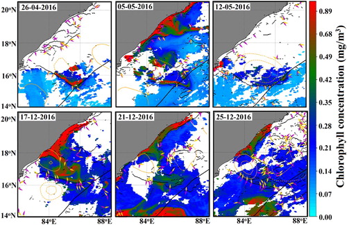
In Case I (Figure 3, upper panel), a strong thermal front with high chlorophyll values can be seen south of 16^oN, where vectors of thermal front and net Ekman transport are aligned almost in the same direction, towards south. During the period 26th April to 12th May 2016, a prominent southward movement of the thermal front can be observed especially in the southwestern part of the front. The frontal arrow indicates the gradient of temperature cold water to hot water. In this case, the cyclonic eddy (cold core) centred at around 16^oN (Figure 4(a)) also plays an important role in distributing the surface chlorophyll. This eddy was weak on 05th April 2016 and was having an amplitude and a radius of 0.06 m and 103 km, respectively. Over the period, it strengthened and was found to have maximum amplitude (0.31 m) and radius (175 km) on 16th May 2016 (Figure 4(a)). Associated changes can be observed in the distribution of chlorophyll and frontal structure also.

Figure 4. The weekly propagation of the eddies, the eddy size is represented by the size of the circle and colour represents amplitude (m) for (a) Case I and (b) Case II. The circle having boundary is indicating the anti-cyclonic eddy. Blue(color) / black(b/w) and red(color) / grey(b/w) lines show the propagation of cyclonic and anti-cyclonic eddies, respectively

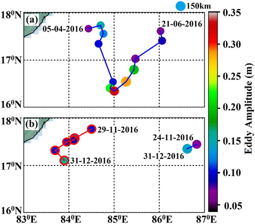
For case II (Figure 3, lower panel), a period of 17th December to 25th December 2016 was chosen where both the vectors are almost in the opposite direction. High chlorophyll water observed along the boundaries of thermal front near to the coast was around 18^oN on 17th December 2017 and subsequently this patch was observed to be dissipating with time. Two things can be observed in this case. First, frontal direction and Ekman transport are in the opposite direction, which suppress the further intensification of front by reducing the thermal gradient. Secondly, the impact of anti-cyclonic eddy formed near the front (Figure 3, lower panel) acts as the opposite force for further intensification of chlorophyll bloom by distributing warm water to cold water regime of the front. Several studies have shown that eddies are good fishing areas (Zainuddin et al. 2008; Lumban-Gaol et al. 2015) and fronts and eddies are also key structures in the habitat of marine fish larvae (Bakun 2006). Along with this, Ekman transport is also supporting the intensification of anti-cyclonic eddy (Figure 4(b), amplitude of the eddy intensified over the period 29th November 2016 (0.1 m) to 31st December 2016 (0.15 m)) by pushing warm water to north-eastern side, which may also result in the dissipation of the chlorophyll patch. Although a cyclonic eddy can be observed on the eastern side of the anti-cyclonic eddy, its impact on chlorophyll and frontal structures is not found to be prominent. This is because this cyclonic eddy is week in comparison to the anti-cyclonic eddy (Figure 4(b)) and hence the impact is not that significant.

In general, an increase in the intensity of front and a significant drift of the frontal filament is observed when front and Ekman transport are aligned in the same direction. If they are not aligned or they are in the opposite direction, Ekman transport suppresses further intensification and drift of thermal fronts.

3.2. Monitoring and forecasting of PFZ by the suggested methodology

A composite map of PFZ is generated using the fishing ground parameters, as explained in section 2, which involves the oceanic features of thermal fronts, upwelling zones, tracked mesoscale eddies and favourable chlorophyll conditions. Defined PFZ regions in the maps are then classified as the regions of fish catches with high and very high probability using the conditions, as explained in Table 1. However, chlorophyll is kept as a mandatory parameter in all the conditions for the accurate identification of PFZ (Solanki et al. 2003; Choudhury et al. 2007; Wilson et al. 2008; Zainuddin et al. 2013). This additional information of high and very high probability of PFZ is to help fishermen to choose suitable PFZ locations according to the fish catch duration, fuel, manpower etc. Figure 5 shows a few examples elucidating the conditions considered for the generation of PFZ maps. Figure 5 is the same as Figure 3 for different dates. Two specific cases are chosen from the figure to explain the high (H) and very high (VH) probability of fish catch, (i) region contains thermal fronts as well as favourable chlorophyll condition (H, light green box) and (ii) region contains thermal fronts, favourable chlorophyll condition as well as a cyclonic eddy (VH, light pink box). As per the suggested methodology, these two regions will be identified as PFZ locations in the map, indicating region 2 as the PFZ of very high probability for the fish catch.

Figure 5. An example showing conditions considered for the generation of PFZ maps. CHL (mg/m³) is shown as a shaded plot, which is overlaid by thermal fronts (thin black lines), cyclonic (dashed contour) and anticyclonic (closed contour) eddies, Ekman transport (yellow(color) / white(b/w) vector) and frontal direction (pink vector(color) / grey(b/w)). The thick black line shows EEZ boundary. The region with high probability (H) and very high probability (VH) are shown in left top and right bottom boxes in figure 5, respectively.

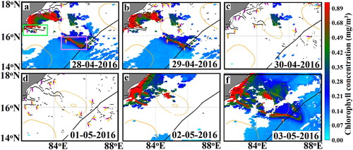
Table 1. Conditions set to filter out regions of fish catches with high and very high probability in PFZ maps.

Ocean conditions in defining PFZ map	Fish catch probability
Thermal fronts, favourable chlorophyll condition, upwelling zones, tracking of cyclonic eddies Or Thermal fronts, favourable chlorophyll condition, tracking of cyclonic eddies	Very High probability (VH)
Thermal fronts, favourable chlorophyll condition Or Favourable chlorophyll condition, upwelling zones	High probability (H)

The next fundamental and more informative step that helps fishermen is regarding the forecasting of the identified fish locations. Since long, the forecasting of PFZ mostly depends only on the wind direction or a likely tendency of PFZ to move according to the prevailing wind conditions (Chandran et al. 2004; Solanki et al. 2005). The method proposed in the paper incorporates various ocean parameters such as ocean surface current, frontal movement in addition to the wind-induced Ekman transport to forecast PFZ. PFZ locations of very high persistence identified using wind and frontal information are then forecasted using information from ocean surface current. Loss of information on chlorophyll is visible for most of the days (Figure 5(c–e) due to cloud coverage and this poses difficulty in PFZ forecasting. The strength of our algorithm is the short-term (up to 2–3 days) forecast of PFZ locations even in the absence of chlorophyll data using other information e.g. relative wind fields and thermal fronts. As per the proposed algorithm, the two specified PFZ regions discussed above (Figure 5) show a chance of persistence since the vectors of front and Ekman transport are aligned in the same direction. PFZ monitoring was only possible for 28th and 29th of April (Figure 5(a,b)) and chlorophyll data were not available for the next three days (Figure 5(c–e)). It can be observed from Figure 5(f) that the PFZ features observed in Figure 5(a,b) are persisted and it is proved that the forecast information given in Figure 5(a,b) is correct even for the cloud-contaminated regions.

3.3. Composite image and final map of PFZ

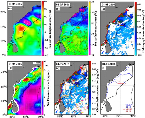
This section provides a comprehensive view of the methodology described in the study to track fishing ground parameters for the accurate detection and forecasting of PFZ locations. Figure 6 shows the final map of PFZ for the day 4th May 2016. Figure 6(a) shows the weekly average of SLA in which cyclonic and anti-cyclonic eddies are demarcated. The continuous and dotted lines are indicating the anti-cyclonic and cyclonic eddies, respectively. It is clear from Figure 6(a) that the western part of the BoB is more prone to eddy activities and the CHL concentrations are found to be maximum in the region of cyclonic eddies (Figure 6(c)). Net Ekman transport is mostly visible along the regions adjacent to coast (Figure 6(d)) and is strong when associated with cyclonic eddies. Strong thermal gradients are also visible mainly along the periphery of cyclonic eddies (Figure 6(b)) and they are associated with large CHL concentration. The PFZ locations were identified using the information from these physical parameters (Figure 6a to 6d) and the final PFZ map has been generated (Figure 6(f)), based on Figure 6(e). In the map, PFZ locations are marked in different colours to demarcate the regions of high and very high probability for the fish catch with the possible status of the PFZ to strengthen (HP, High persistence) or to weaken (LP, Low persistence) in future. H (high probability) and VH (very high probability) demarcate the probability of PFZ.

Figure 6. (a) SSHA(m) overlaid with eddy boundaries (white contour, continuous for anti-cyclonic and dotted for cyclonic eddies), (b) SST(^oC)overlaid with thermal fronts (thin black line) and frontal direction (arrows), (c) chlorophyll concentration(mg/m³), (d) net Ekman transport with its direction (black arrow), (e) comprehensive image of the input parameters. The CHL shown as a shaded plot is overlaid by thermal fronts (thin black lines), cyclonic (dashed contour) and anticyclonic (closed contour) eddies, Ekman transport (yellow(color) / white(b/w) vector) and frontal direction (pink(color) / grey(b/w) vector), (f) Final PFZ map derived from the image is shown as Figure 6e. Very high probability (VH) and high probability (H) regions with high persistence (HP) and low persistence (LP). The thick black line shows EEZ boundary.

3.4. Validation of the proposed algorithm for PFZ

After generating PFZ maps, obviously the next step was to validate the identified PFZ locations. It is a mandatory step in every technique before its implementation and here PFZ validation involves two steps. The first step is to validate the monitored PFZ regions with in situ fish catch data for the period January to March 2017. The second step involves the validation of the forecasting method.

3.4.1. Validation of the monitored PFZ regions

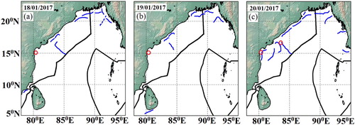
Available in situ fish catch locations are overlaid over PFZ map and are shown as Figure 7. Only the dates of moderate fish catch (> 50 kg/h) are chosen for the validation (18th January 2018 to 20th January 2018) and the fish catch locations are indicated as red circle in the figure. The dominant fishes caught by trawl net operation and long line operation in the study area were mackerels, carangids, sardines, Leiognathids, anchovies, clupeoids, catfishes, Priacanthids, rays, ribbonfish, squids, sharks, barracudas, etc. It is stated that PFZ advisories were not possible over some fish locations due to cloud cover (Figure 7(a,b)). The persistence forecast of PFZ using data from the previous day can be used for these cases. It can be seen from Figure 7(c) that locations of actual fish catch coincide with identified PFZ, which support the accuracy of the suggested methodology. The significance of the satellite images in delineating the multifarious dynamics of PFZ is demonstrated in the present study by exploring various ocean conditions that favours fish availability.

Figure 7. The 3-consecutive dates of PFZ images are overlaid with the in situ fish catch data locations as circles. The thick black line shows EEZ boundary. PFZ locations with high probability with high persistence are marked by continuous lines and high probability with low persistence of PFZ location is marked by dashed lines. PFZ locations with very high probability were not available on these dates.

3.4.2. Validation of the PFZ forecast

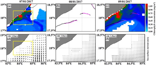
The proposed methodology for PFZ forecast involves two parts; (i) to identify PFZ regions of high persistence, i.e. (H, HP and VH, HP regions) and (ii) to forecast the possible propagation of those identified PFZ regions using current information on t₀ day. The first part is explained in detail in earlier sections. In the second part, the drift of identified PFZ regions is computed using the ocean surface current information on t₀th day (forecasted PFZ). Figure 8 shows thermal fronts overlaid on CHL images for the three consecutive days (7th, 8th and 9th January 2017). Two PFZ regions (VH with HP) in the yellow box (Figure 8(a)) are taken for the validation. Figure 8(b,c) show the monitored PFZ (black line) and forecasted PFZ (pink line) for 8th and 9th January 2017, respectively. Forecasted PFZs are then compared with the persistence PFZ. Here the persistence PFZ means the PFZ on t₀^th day is supposed to persist at the same location for the next two days (t₀+1 and t₀+2 days). But in reality the feature will be drifting along with the surface advective movements. The average distance between forecasted PFZ and persistence PFZ has been computed for the subsequent days (t₀+1 and t₀+2) and the values are coming 0.76 and 1.14 km, respectively. The actual drift has been calculated and the values are coming 0.72 and 1.082 km for t₀+1 and t₀+2, respectively.

Figure 8. (Upper panel) Thermal fronts are overlaid on CHL images for the three consecutive days (7th, 8th and 9th January 2017). Monitored PFZ for the corresponding dates is marked as black line. Pink line(color)/ grey(b/w) in (b) and (c) shows the corresponding forecasted PFZ using the information from (a). (Lower panel) ISRO currents for the corresponding dates. Plots (b, c, e and f) show the enlarged view of the yellow box shown in (a and d).

4. Conclusion and future scope of the work

In the present study, an algorithm has been developed to track fishing ground parameters such as eddies, thermal fronts, CHL etc. for the proper monitoring and forecasting of the PFZ regions in the BoB. For this, a modified methodology has been suggested over the conventional method that uses only satellite-derived SST and CHL. The suggested approach attempts to establish the link between fish catch availability and various ocean parameters available from satellites, such as CHL, SST, SSHA, ocean surface currents and wind vectors. In this study, it has been shown that once the productive zones are identified based on the prevalent eddy information along with SST front and CHL, the Ekman transport obtained from the relative wind direction provides valuable information on the persistence of such feature and their propagation. Hence this technique also provides the probability of the persistence of the identified PFZ, even under cloudy conditions. The results are compared with available limited insitu fish catch data. Results showed the efficiency of the PFZ algorithm in monitoring possible fish catch locations.

Since satellite datasets, especially CHL and SST, suffer from the cloud masking and also the availability of fish catch data was limited, we could not perform a detailed validation of the proposed approach. The purpose of this paper, however, was to put forth a new methodology that can have a persistent forecast capability. A detailed assessment is proposed to be performed in future work. To circumvent the cloud cover issue in CHL and SST, a synergistic approach is planned to be used in PFZ advisory based on satellite and numerical model. The analysed and forecasted fields of SST, CHL and surface ocean currents from the coupled bio-physical model will be used in the PFZ algorithm. One advantage of the model fields is its continuous availability, which will help to provide PFZ advisories without any gap. A continuous validation of ocean parameters from the model with satellite parameters will be routinely done to assure the robustness of the model in forecasting the ocean parameters. To increase the quality of PFZ advisory, a more advanced exercise is planned to be executed. Quality of the model parameters will be improved by assimilating the satellite-derived parameters into the model and this assimilated coupled model will be used to provide inputs into the PFZ algorithm. In future, we propose to use very high-resolution-coupled bio-physical model forecasts synergistically with satellite observations to explore the benefits of synergistic methods for PFZ advisory.

Acknowledgements

The authors would like to express their gratitude to Shri. D. K. Das, Director, Space Applications Centre, and Dr Raj Kumar, Deputy Director, Earth, Ocean, Atmosphere, Planetary Sciences and Applications Area and Dr C. M. Kishtawal, Group Director, AOSG for their support, encouragement and valuable suggestions. Dr Neeraj Agarwal is greatly acknowledged for his comments and suggestions that helped in improving the manuscript significantly. The fish catch data received from Fishery Survey of India, Mumbai are sincerely acknowledged as part of the SAC TDP ‘SAMUDRA’ Program.

Disclosure statement

No potential conflict of interest was reported by the authors.

References

- Abbott MR, Zion PM. 1985. Satellite observations of phytoplankton variability during an upwelling event. Cont Shelf Res. 4(6):661–680.
- Ardianto R, Setiawan A, Hidayat J, Zaky A. 2017. Development of an automated processing system for potential fishing zone forecast. IOP Conference Series: Earth and Environmental Science. 54(1):012081.
- Bakun A. 2006. Fronts and eddies as key structures in the habitat of marine fish larvae: opportunity, adaptive response and competitive advantage. Sci Mar. 70(S2):105–122.
- Balaguru B, Ramakrishnan S, Vidhya R, Thanabalan T. 2014. A Comparative study on utilization of multi-sensor satellite data To detect potential fishing zone (PFZ). Int Arch Photogramm Remote Sens Spatial Inf Sci. 40(8):1017.
- Belkin IM, Cornillon PC, Sherman K. 2009. Fronts in large marine ecosystems. Prog Oceanogr. 81(1-4):223–236.
- Carpenter SR, Kitchell JF, Hodgson JR. 1985. Cascading trophic interactions and lake productivity. BioScience. 35(10):634–639.
- Chandran RV, Solanki H, Dwivedi R, Nayak S, Jeyaram A, Adiga S. 2004. Studies on the drift of ocean colour features using satellite-derived sea surface wind for updating potential fishing zone. Int J Remote Sens. 33(2):122–128.
- Chavez F, Strutton P, Friederich G, Feely R, Feldman G, Foley D, McPhaden M. 1999. Biological and chemical response of the equatorial Pacific Ocean to the 1997–98 El Niño. Science. 286(5447):2126–2131.
- Chelton DB, Schlax MG, Samelson RM. 2011. Global observations of nonlinear mesoscale eddies. Prog Oceanogr. 91(2):167–216.
- Choudhury S, Jena B, Rao M, Rao K, Somvanshi V, Gulati D, Sahu S. 2007. Validation of integrated potential fishing zone (IPFZ) forecast using satellite based chlorophyll and sea surface temperature along the east coast of India. Int J Remote Sens. 28(12):2683–2693.
- Dwivedi R, Solanki H, Nayak S, Gulati D, Somvanshi V. 2005. Exploration of fishery resources through integration of ocean colour with sea surface temperature: Indian experience. Int J Remote Sens. 34(4):430–440.
- Falkowski PG, Ziemann D, Kolber Z, Bienfang PK. 1991. Role of eddy pumping in enhancing primary production in the ocean. Nature. 352(6330):55.
- Field CB, Behrenfeld MJ, Randerson JT, Falkowski P. 1998. Primary production of the biosphere: integrating terrestrial and oceanic components. Science. 281(5374):237–240.
- Frenger I, Münnich M, Gruber N. 2018. Imprint of Southern Ocean mesoscale eddies on chlorophyll. Biogeosciences. 15(15):4781–4798.
- George G, Krishnan P, Dam Roy S, Sarma K, Goutham Bharathi M, Kaliyamoorthy M, Krishnamurthy V, Srinivasa Kumar T. 2013. Validation of potential fishing zone (PFZ) forecasts from Andaman and Nicobar Islands. Fish Technol. 50:1–5.
- Islam MS. 2003. Perspectives of the coastal and marine fisheries of the Bay of Bengal, Bangladesh. Ocean Coast Manag. 46(8):763–796.
- Kahru M, Gille S, Murtugudde R, Strutton P, Manzano-Sarabia M, Wang H, Mitchell B. 2010. Global correlations between winds and ocean chlorophyll. J Geo Res: Oceans. 115(C12):1–11.
- Kamei G, Felix JF, Shenoy L. 2014. Trends of potential fishing zones (PFZs) along the Mumbai coast, Maharashtra. Indian J Fisheries. 61(2):140–142.
- Kostianoy AG, Ginzburg AI, Frankignoulle M, Delille B. 2004. Fronts in the Southern Indian ocean as inferred from satellite sea surface temperature data. J Mar Sys. 45(1-2):55–73.
- Kurian J, Colas F, Capet X, McWilliams JC, Chelton DB. 2011. Eddy properties in the California current system. J Geo Res: Oceans. 116(C8):1–18.
- Laurs RM. 1993. Integration of various satellite derived oceanography information for the identification of potential fishing zones. Lecture notes of international workshop on application of satellite remote sensing for identifying and forecasting potential fishing zones in developing countries, Hyderabad, India, 7–11 December 1993.
- Lumban-Gaol J, Leben RR, Vignudelli S, Mahapatra K, Okada Y, Nababan B, Mei-Ling M, Amri K, Arhatin RE, Syahdan M. 2015. Variability of satellite-derived sea surface height anomaly, and its relationship with Bigeye tuna (Thunnus obesus) catch in the eastern Indian ocean. Eur J Remote Sensing. 48(1):465–477.
- Mahadevan A. 2014. Ocean science: eddy effects on biogeochemistry. Nature. 506(7487):168.
- Mahadevan A. 2016. The impact of submesoscale physics on primary productivity of plankton. Ann Rev Mar Sci. 8:161–184.
- Mansor S, Tan C, Ibrahim H, Shariff ARM. 2001. Satellite fish forecasting in South China sea. Paper presented at the 22nd Asian Conference on Remote Sensing. 5:9.
- Mason E, Pascual A, McWilliams JC. 2014. A new sea surface height–based code for oceanic mesoscale eddy tracking. J Atmos Ocean Technol. 31(5):1181–1188.
- McGillicuddy Jr DJ, Robinson A, Siegel D, Jannasch H, Johnson R, Dickey T, McNeil J, Michaels A, Knap A. 1998. Influence of mesoscale eddies on new production in the Sargasso Sea. Nature. 394(6690):263.
- Mittelbach GG, Ballew NG, Kjelvik MK. 2014. Fish behavioral types and their ecological consequences. Can J Fish Aquat Sci. 71(6):927–944.
- Nayak S, Solanki H, Dwivedi R. 2003. Utilization of IRS P4 ocean colour data for potential fishing zone—a cost benefit analysis. Int J Remote Sens. 32(3):244–248.
- Naylor RL, Goldburg RJ, Primavera JH, Kautsky N, Beveridge MC, Clay J, Folke C, Lubchenco J, Mooney H, Troell M. 2000. Effect of aquaculture on world fish supplies. Nature. 405(6790):1017.
- Owen RW. 1981. Fronts and eddies in the sea: mechanisms, interactions and biological effects. Analysis of Marine Ecosystems. 197–233.
- Pillai N, Abdussamad E. 2008. Development of tuna fisheries in Andaman and Nicobar Islands. Proc Brainstorming Sess Dev Isl Fish. 23–34.
- Rao R, Sivakumar R. 2003. Seasonal variability of sea surface salinity and salt budget of the mixed layer of the north Indian Ocean. J Geo Res: Oceans. 108(C1):9-1–9-14.
- Reese DC, O’Malley RT, Brodeur RD, Churnside JH. 2011. Epipelagic fish distributions in relation to thermal fronts in a coastal upwelling system using high-resolution remote-sensing techniques. ICES J Mar Sci. 68(9):1865–1874.
- Sahu K, Baliarsingh S, Srichandan S, Lotliker A, Kumar T. 2012. Validation of PFZ advisories – a case study along Ganjam coast of Orissa, East Coast of India. Indian Streams Res J. 1(12):1–6.
- Sankari S. 1996. Export prospects for Indian marine products. Export Potential Indian Agric. 383:1–25.
- Schott FA, McCreary Jr JP. 2001. The monsoon circulation of the Indian Ocean. Prog Oceanogr. 51(1):1–123.
- Shankar D, Vinayachandran P, Unnikrishnan A. 2002. The monsoon currents in the north Indian ocean. Prog Oceanogr. 52(1):63–120.
- Sharma G. 1978. Upwelling off the southwest coast of India. Indian J Mar Sci. 7(4):209–218.
- Sharma R, Agarwal N, Chakraborty A, Mallick S, Buckley J, Shesu V, Tandon A. 2016. Large-scale air-sea coupling processes in the Bay of Bengal using space-borne observations. Oceanography. 29(2):192–201.
- Sikhakolli R, Sharma R, Basu S, Gohil B, Sarkar A, Prasad K. 2013. Evaluation of OSCAR ocean surface current product in the tropical Indian Ocean using in situ data. J Earth Syst Sci. 122(1):187–199.
- Singh A, Gandhi N, Ramesh R, Prakash S. 2015. Role of cyclonic eddy in enhancing primary and new production in the Bay of Bengal. J Sea Res. 97:5–13.
- Sissenwine MP. 1984. Why do fish populations vary? Exploitation of marine communities. Dahlem Workshop Report, Springer, Berlin, Heidelberg. 32:59–94.
- Solanki H, Dwivedi R, Nayak S, Jadeja J, Thakar D, Dave H, Patel M. 2001. Application of ocean colour monitor chlorophyll and AVHRR SST for fishery forecast: Preliminary validation results off Gujarat coast, northwest coast of India. Int J Remote Sens. 30(3):132–138.
- Solanki H, Dwivedi R, Nayak S, Somvanshi V, Gulati D, Pattnayak S. 2003. Fishery forecast using OCM chlorophyll concentration and AVHRR SST: validation results off Gujarat coast, India. Int J Remote Sens. 24(18):3691–3699.
- Solanki H, Mankodi P, Nayak S, Somvanshi V. 2005. Evaluation of remote-sensing-based potential fishing zones (PFZs) forecast methodology. Cont Shelf Res. 25(18):2163–2173.
- Suárez-Morales E, Carrillo A, Morales-Ramírez A. 2013. Report on some monstrilloids (Crustacea: Copepoda) from a reef area off the Caribbean coast of Costa Rica, Central America with description of two new species. J Nat Hist. 47(5-12):619–638.
- Thomas LN. 2005. Destruction of potential vorticity by winds. J Phys Oceanogr. 35(12):2457–2466.
- Thomas LN, Lee CM. 2005. Intensification of ocean fronts by down-front winds. J Phys Oceanogr. 35(6):1086–1102.
- Venegas RM, Strub PT, Beier E, Letelier R, Thomas AC, Cowles T, James C, Soto-Mardones L, Cabrera C. 2008. Satellite-derived variability in chlorophyll, wind stress, sea surface height, and temperature in the northern California current system. J Geo Res: Oceans. 113:C3.
- Wickett WP. 1967. Ekman transport and zooplankton concentration in the north Pacific Ocean. J Fisheries Board Canada. 24(3):581–594.
- Wijesekera HW, Shroyer E, Tandon A, Ravichandran M, Sengupta D, Jinadasa S, Fernando HJ, Agrawal N, Arulananthan K, Bhat G. 2016. ASIRI: an ocean–atmosphere initiative for Bay of Bengal. Bull Am Meteorol Soc. 97(10):1859–1884.
- Wilson C, Morales J, Nayak S, Asanuma I, Feldman G. 2008. Ocean-colour radiometry and fisheries. Why Ocean Colour. 47–58.
- Yamanaka I. 1988. The fisheries forecasting system in Japan for coastal pelagic fish. Food & Agriculture Org. 301:1–80.
- Zainuddin M, Nelwan A, Farhum SA, Hajar MAI, Kurnia M. 2013. Characterizing potential fishing zone of Skipjack Tuna during the Southeast monsoon in the Bone Bay-Flores Sea using remotely sensed oceanographic data. Int J Geo. 4(01):259.
- Zainuddin M, Saitoh K, Saitoh SI. 2008. Albacore (Thunnus alalunga) fishing ground in relation to oceanographic conditions in the western north Pacific Ocean using remotely sensed satellite data. Fish Oceanogr. 17(2):61–73.
- Zuidema P. 2003. Convective clouds over the Bay of Bengal. Mon Weather Rev. 131(5):780–798.