Evaluation of extreme storm waves in the Black Sea

ABSTRACT

The objective of the present study is to give a contribution to the extreme wave climate assessment in the Black Sea, as studies of extreme storm waves are of great interest for coastal protection and maritime traffic. High resolution wind wave data sets are used to investigate trends and variability of the characteristics of extreme storm waves. Two different methodologies (Eulerian and Lagrangean) are applied to 30 years of wave hindcast from 1987 to 2016, over the Black Sea to identify extreme storm waves and also to assess the extreme wave climate. Using the Eulerian methodology, it is observed that extreme storm waves are seasonal, being more frequent during the winter and almost non-existent during the summer. Also, that some areas, as the south-eastern region of the Black Sea more prone to storm generation, in particular, during winter and autumn. For the seven locations near the coast, a considerable inter-annual variability is found in extreme values, but not so much in the mean. Statistical significance in trend adjustment was only found in two locations in the north-western coast, for extreme values. Using a Lagrangean methodology, an inter-annual variability in all storm characteristics that is found, more marked in the annual number of wave storms, maximum area affected by storm waves and maximum length, and less marked for maximum Hs in the storm waves and storm lifetime.

KEYWORDS:

• Black Sea
• extreme storm
• storm track
• Lagrangean approach

Introduction

The general atmospheric circulation in the Black Sea region is influenced by the configuration of the Azores and the Siberian high pressure centres and the Asian low pressure area. Wind speed decreases in general from west to east. In winter north-eastern winds prevail. Eastern winds are predominant only in south-eastern areas. However, during the summer, the prevailing wind blows from northwest, being stronger offshore than near the coast (Valchev et al. 2012; Arkhipkin et al. 2014). Better knowledge of the wave climate is useful for a wide range of practical applications related to the marine and coastal activities, such as offshore platforms, the design of marine structures, the assessment of flooding risk and the evaluation of wave energy resources (Rusu and Guedes Soares 2012; Bento et al. 2014; Laugel et al. 2014). Extreme waves, storms and storminess, in general, have a major impact on coastal populations and ecosystems (Li et al. 2014). The occurrences of such phenomena determine the short-term evolution of coast by beach erosion or destruction of infrastructures (Trifonova et al. 2012). Also, an increased understanding about storm variability and trends (Davies et al. 2017) allows improved preparedness to deal with these extreme events and mitigate impacts on populations and the environment (Kislov et al. 2016).

Several studies have been made about the wave conditions in the Black Sea, such as the hindcast of Cherneva et al. (2008) conducted with the scope of the HIPOCAS project (Guedes Soares 2008), where they used the WAM model to generate a database of 33 years. An overview of wave regimes of the Black Sea can be found in Arkhipkin et al. (2014). These authors also analysed the wind and wave in the Black Sea. For that wave modelling using the SWAN model forced by the NCEP/NCAR reanalysis data set with a threshold of 2 m was used. There are also several studies about the storm conditions in the Black Sea, such as the study by Valchev et al. (2012). They studied the trends and changes in the occurrence and magnitude of marine storms in the western Black Sea during 63 years, trying also to find some possible connections to the NAO index. The wave climate at the Danube delta coast is also important for navigation, being studied by Ivan et al. (2012). Recently, Zăinescu et al. (2017) investigated the storm climate on the Danube delta coast, using wind and wave data and developed a storm severity index.

The storm climate and related ocean roughness depend on the storm tracks, intensity, duration, and frequency of occurrence (Dupuis et al. 2006).

The purpose of this work is to contribute to the characterisation of the present wave climate in the Black Sea, and it represents a follow up of the study initiated by Rusu et al. (2018a). Now, a particular attention is directed to the occurrence of extreme storm events and to investigate trends and variability of the characteristics of extreme storms, identified using both Lagrangean and Eulerian methodologies.

A wave storm can be considered as an event in both space and time where the significant wave height (Hs) rises above a predetermined critical level. The usual methodology is an Eulerian approach based on joint analysis of the variability of the field of significant wave height at a given location.

The availability of databases with spatial information of the characteristics of the wave fields, covering periods of several decades, that can be obtained from large-scale simulations (e.g. Campos and Guedes Soares 2016), allows an assessment of both the temporal and the spatial evolution of wave storms, providing a Lagrangean description of storm characteristics. This methodology is widely used in the atmospheric sciences where, for example, extra-tropical cyclones have been the subject of climatological studies (Trigo 2006), as the location of the storm track has an influence on local weather.

In the sea, wind wave storms have a major impact on coastal areas but also on offshore structures and ship routes. The knowledge of predominant storm tracks, their characteristics, including trends and variability (Menendez et al. 2009) can give a greater value to the existing wave climate information. An example of how information about storms and storm tracks can be used is indicated by Lopatoukhin et al. (2013) and Boukhanovsky et al. (2003). Another example is for ships that cross the ocean in predefined routes (Vettor and Guedes Soares 2015) where the a priori knowledge of the wave storm’s dynamical characteristics can help the masters to avoid the dangerous areas (Vettor and Guedes Soares 2016).

This alternative process, to identify and track a storm along its trajectory, assessing the modifications of their characteristics over time was described in Bernardino et al. (2008) and Bernardino and Guedes Soares (2015, 2016) and had previously been applied to a closed area, the Barents Sea by Boukhanovsky et al. (2003).

Data and methodology

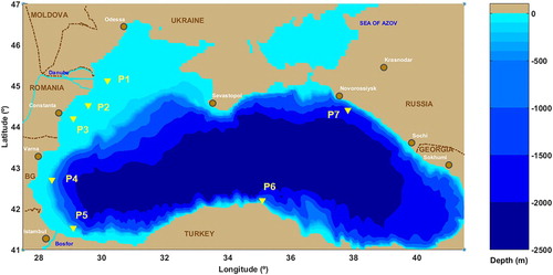
In the present work, a 30-year wave hindcast dataset (from 1987 to 2016) based on the SWAN (acronym from Simulating WAve Nearshore, Booij et al. 1999) model results over the Black Sea is analysed (Rusu 2015; Rusu 2019). The SWAN model was implemented in the entire basin of the Black Sea, also including the Sea of Azov (Figure 1). The computational and bathymetric grids coincide and their resolution in the geographical space is 0.08° × 0.08°. The origin of the grids corresponds to the lower left corner point with the coordinates 27.5°E/41.0°N. The x-direction (longitude) extends 14°, while the y-direction (latitude) extends 6°. The SWAN simulations were carried out in non-stationary mode (using a time step of 10 min), the third generation mode for wind input, quadruplet interactions and whitecapping. In spectral space, the full circle was considered (divided into 36 bins) and 30 frequencies logarithmically between 0.05 and 1.0 Hz. All outputs of the SWAN model have a temporal resolution of 3 h. In this study, only Hs simulated by SWAN are considered.

Figure 1. Bathymetry of the Black Sea (from General Bathymetric Chart of the Oceans – GEBCO) and location of points P1–P7.

The wind fields at 10 m (u10 and v10 wind components) provided by the US National Centers for Environmental Prediction, Climate Forecast System Reanalysis (NCEP-CFSR) and Climate Forecast System Version 2 (NCEP-CFSv2) (Saha et al. 2014) are used to force the wave model. In some previous studies, the results of the SWAN model in this sea were validated against in-situ and remotely sensed measurements (Butunoiu and Rusu 2012; Rusu et al. 2014a, 2014b; Rusu 2015), providing an evaluation of the quality of the numerical simulations over the entire basin scale. This represents a follow up on previous studies, being focused on the analysis of the storm conditions. From the available parameters, only significant wave height data, with 3 h temporal resolution and 0.32° by 0.32° spatial resolution, was considered to evaluate extreme wave events in this region.

Various studies define storms as high intensity events of the significant wave height time series above a given level (Petruaskas and Aagaard 1971; Haring et al. 1976; Angelides et al. 1981; Laface et al. 2015). The statistics of storm duration (see, e.g. Jardine and Latham 1981; Graham 1982; Mathiesen 1994), and the corresponding maximum significant wave height in a storm (as the measure of storm intensity) are studied in Borgman (1973), Boukhanovsky et al. (1988), Laface and Arena (2016), Bernardino et al. (2008) and Bernardino and Guedes Soares (2015, 2016).

The time series of significant wave height (measurements or model results) at a given location can be used for Eulerian analysis of the wave storms. This is a classical approach to statistical analysis of the wave storms. The information obtained in this approach is especially related to the frequency of events, their duration and intensity, and an estimate of extreme conditions, at given locations resulting in a joint analysis of multivariate time series of intensities and durations of wave storms at each point. In theory, this joint analysis of the wave storm durations would identify the same storm in several places. On the other hand, the characteristics of the wave storms are changing over time and to identify the points affected by the same storm is a very difficult process.

The reanalysis databases provide information of the wave characteristics at large-scales and during periods of several decades. This allows an assessment of the spatiotemporal evolution of significant wave height fields. Fundamentally information concerning the wave storm variability over the ocean is available in an approach that is traditional for meteorological researches, where the spatiotemporal variability of cyclones is considered. The dynamics of wave storms as spatial structures in а field is considered by the Lagrangean approach. With respect to the classical definition of storms in a wave time series, the wave storm area $\left(\mathrm{\Omega }\right)$ is analysed in the space domain, for each time $t$, as the constrained set of grid points (Boukhanovsky et al. 2003; Bernardino et al. 2008) where(1) $\mathrm{\Omega }\left(t\right)=\left\{\left(x,y\right),h\left(x,y,t\right)>z\right\},$(1) with h(x,y,t) also representing the significant wave height field and z the wave storm definition threshold.

The function(2) $W\left(x,y,t\right)=\left\{\begin{array}{c}\begin{array}{c}h\left(x,y,t\right)-z,\left(x,y\right)\in \mathrm{\Omega }\left(t\right)\\ \end{array}\\ 0,\left[\left(x,y\right)\notin \mathrm{\Omega }\left(t\right)\right]\mathrm{o}\mathrm{r}\left[t\notin \left[0,D\right]\right]\end{array}\right.$(2) for each time instant $0\le t\le D$, where $D$ is the total duration (or life time) of the wave storm above the level $z$, may be interpreted as a spatial stochastic pulse. Pulse dynamics $W(x,y,t)$ depend on a set of parameters $\mathrm{\Xi }\left(t\right)$ that characterise the spatial shape of the wave storm. It should be noted that the pulse evolves both in time and space.

Both approaches to wave storm dynamics (Eulerian and Lagrangean) represent in fact the same physical situation in different ways. For practical reasons, and for each concrete problem, one approach could be more appropriate than the other.

In the present work, both methodologies were applied to the wave data set, in order to perform a study of extreme storm waves affecting the Black Sea. In the Lagrangean methodology, a threshold of 5 m for significant wave height and a minimum duration of 12 h were imposed to perform the wave storm identification. This type of restrictions was used when analysing wave storms in other locations. Thus, Bernardino and Guedes Soares (2015, 2016) used a threshold of 7 m when analysing wave storms in the North Atlantic. In the Black sea, with a less energetic environment, Arkhipkin et al. (2014) used a threshold of 2 m.

Results

Local wave climate

The wave climate in the Black Sea was evaluated in seven locations near the coast (see Figure 1), chosen in areas more affected by wave storms as indicated by previous studies (Onea and Rusu 2017; Galabov and Chervenkov 2018; Rusu et al. 2018a). These points are also in the vicinity of some important harbours.

Location P1 is the northern one (near the Danube Delta) and it is followed by locations P2–P7 anti-clockwise. P7 is located near the Sea of Azov. The first three points are in front of the Romanian nearshore where the maritime traffic is high due to the Constanta port is one of the major ports at the Black Sea, and also the Sulina port, at the mouth of the Danube River, is connected to the waterways of Europe. In the proximity of the Bosphorus strait (P5) is also important to evaluate the wave climate, being the link of the Black Sea with other oceans. Significant wave height time series were extracted for each location. Based on these data the mean monthly values were computed and the results are plotted in Figure 2. A strong seasonal cycle can be seen in all the locations, with lower Hs values in the summer and higher in the winter. The difference among locations is more marked in summer/autumn than in winter/spring, in particular, between July and October.

Figure 2. Seasonal cycle of Hs, for the seven locations.

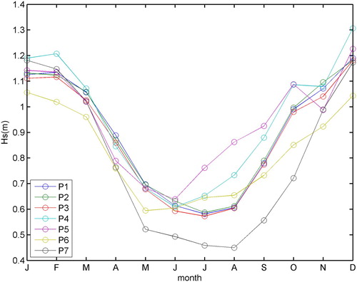
Locations P1–P3 are located close together and show a very similar annual cycle. P5 located in the southwestern coast, shows relative high values during the summer, in comparison with other locations. At the P6 location, the less marked seasonal cycle of Hs is observed, with the difference between summer and winter of less than 0.5 m. The month when the minimum Hs is obtained, the month of May, unlike the other locations that presented lower monthly values between June and August.

Considering all the three hourly data in each location, a statistical analysis was performed. Table 1 shows the results obtained for location P1–P7 regarding mean value, standard deviation, the maximum value in the 30 years period under consideration as well as the 95th and 99th percentiles. In general, the mean Hs takes values less than 1 m and the standard deviation values between 0.63 and 0.78 m. Maximum values can be observed between 6.52 m (P2) and 10.54 m (P5). P1–P3 located in the same region present similar statistics, not only in mean and variability but also regarding extreme values.

Table 1. Statistic evaluation of the Hs in the seven selected locations (mean, standard deviation, 95th percentile, 99th percentile, and maximum values) for the period 1987–2016.

Hs (m)	P1	P2	P3	P4	P5	P6	P7
Mean	0.89	0.90	0.88	0.94	0.94	0.82	0.79
Std	0.64	0.64	0.64	0.77	0.78	0.63	0.73
P95	2.16	2.17	2.13	2.43	2.42	2.06	2.25
P99	3.22	3.15	3.27	4.06	4.05	3.2	3.75
Max	7.09	6.52	7.06	8.31	10.54	7.20	9.52

Points P4 and P5, also located in the western Black Sea, but further south, have statistical values that are similar to each other except for the absolute maximum that that is much higher for P5 than for P4, by more than 2 m. P6 and P7 located in central and north-eastern coasts respectively, show lower mean values than the other locations, in particular, P7. P6 shows variability and extremes similar to P1 to P3, but P7, although showing lower mean value, presents higher variability and accordingly higher extremes compared.

In order to further characterise the wave climate in the Black Sea, the 10, 20, 50 and 100 year return periods, in locations P1–P7 were computed. When it comes to deal with extreme values, it is considered the largest and the smallest values from a sample with size n within a known population. Therefore, each of the largest or smallest value will have its own probability distribution, which could be an exact or an asymptotic distribution. The asymptotic distributions of extremes are approximate distributions, whose characteristic parameters depend upon the number of observations, being the approach, all the better the higher that number. A necessary condition for the use of such models is the independence of the observed values. The extreme value distribution commonly referred to in the literature and used in this study was the Type I: Fisher-Tippet, Gumbel, defined by:(3) $F\left(x\right)=\exp \left[-\exp \left(-\left(x-a\right)/b\right)\right]x\in [-\mathrm{\infty },+\mathrm{\infty }],$(3) where a = −B/A and b = 1/A are the characteristic parameters, location and scale respectively and A and B are estimated by the Least Squares method. The Gumbel distribution was fitted with a 5-day maximum time series, and the distribution parameters were computed using the L-moments (Lucas et al. 2017). The maximum value, each five days was adopted in order to decrease the correlation among successive observations as is required for adjusting probability distributions to sets of independent data. The results obtained are presented in Table 2.

Table 2. Return values for 10, 20, 50 and 100 years return periods, for Hs in the seven selected locations.

Return periods	P1	P2	P3	P4	P5	P6	P7
10-years	7.50	7.35	7.45	9.10	9.54	8.28	9.54
20-years	8.00	7.84	7.93	9.73	10.21	8.85	10.22
50-years	8.65	8.46	8.60	10.54	11.07	9.58	11.11
100-years	9.1	8.93	9.08	11.15	11.71	10.13	11.77

It can be seen that locations P1, P2 and P3 show very similar return values for the different return periods, in comparison with the other four locations. Return values for 10 years take values from 7.35 m (P2) to 9.54 m (P5 and P7), and for the 100 years, values from 8.93 m (P2) to 11.77 (P7). P2 shows always the lowest return values and P7 the highest.

With the aim to analyse the long-term variability and trends of Hs in the Black Sea, the annual mean and extreme values (95th and 99th percentiles) were computed and plotted for each location. A linear trend was adjusted and the slope computed is presented in Table 3. It can be seen that with the exception of location P6, all other locations present positive slope values, indicating an uprising trend in annual values, more marked in extremes than in the annual mean.

Table 3. Slope values (in cm per decade) of the linear trend adjusted to the annual mean, 95th percentile and 99th percentile, values for each of the seven locations.

Location	Mean	P95	P99
P1	2.1	8 . 3	17.1
P2	1.5	6.1	20
P3	1.3	6.8	14.2
P4	0.6	5.0	14.4
P5	0.3	1.0	9.1
P6	−0.1	−2.6	5.0
P7	0.7	7.6	14.9

Bold values are statistically significant at 95% level.

Regarding the annual mean values, it can be seen that although the slope values are positive, they are very low showing an increment of 2.1 cm per decade at most. Extreme annual values, however, show a more marked increase during these 30 years, with 99th annual percentile showing slope values more than twice the ones found for 95th percentile. Mann-Kendall test for trends applied to the annual time series showed that only the annual 95th percentile for P1 and 99th percentile for P2 (in bold) are significant at 95% level.

Figures 3 and 4 show the time series of annual mean, 95th percentile and 99th percentile of Hs in the locations P2 and P5. At P2 a high inter-annual variability can be observed for the annual extremes, but no so much for the annual mean value. Superimposing a five years running mean, in order to highlight long term fluctuations, some variability can still be seen in the 99th percentile but this variability is smoothed for the 99th percentile and annual mean. The upwards linear trend is clearer in annual 99th percentile than in other statistics.

Figure 3. Annual mean, 95th percentile and 99th percentile (dashed line), five year running mean (solid line) linear trend (full line) of Hs for location P2.

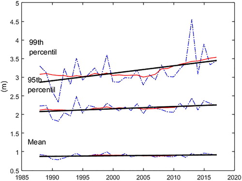
Figure 4. Annual mean, 95th percentile and 99th percentile (dashed line), five year running mean (solid line) linear trend (full line) of Hs for location P5.

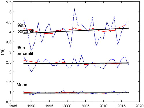
Observing Figure 4, where mean, 95th and 99th percentile annual time series obtained for P5 are presented, it can be seen that the inter-annual variability is very low. As regards the adjusted linear trends, only the one obtained for the 99th percentile shows a positive slope as the ones obtained for 95th percentile and annual mean are almost horizontal, indicating an absence of any positive trend. Evaluating the linear trend of mean, P99 and P95 percentiles values for location P1, a positive uprising trend can be observed in particular in extreme annual values.

Variability of the wave conditions

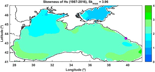
The variability of the wave conditions in the Black Sea was evaluated based on the SWAN model results with a 3 h temporal resolution. An analysis of the spatiotemporal variability of Hs was performed using various statistical indexes. In order to estimate the impact from extreme events on the Hs datasets, a higher moment of the data was computed, namely the skewness (Sk). This index will help to gain information about the degree of asymmetry of Hs distribution around its mean and the potential influence by extremes, and how often they occur, as described in Guedes Soares et al. (2004). This index was determined at each point of the computational domain of the SWAN model, for the entire 30-year period, and it indicates the existence of extremes. In the areas with increased values of Sk the Hs time series are non-symmetric, with small mean values and long heavy tails, that usually characterise an unstable behaviour. For the computation of Sk the following relationship was used:(4) $Sk=\frac{N^{-1}{\sum }_{i=1}^N{\left(x_i-\overline{x}\right)}^3}{{\sigma }^3}$(4) where x is the time series of the parameter analysed (here is Hs), σ is the standard deviation, the over bar denotes average and N the number of the size of the sample and (in this case N represents the number of the model output in each point of the computational domain for the entire 30-year period).

The corresponding results are illustrated in Figure 5. The lowest values of skewness are encountered in the Azov Sea and also in the north-western part of the basin, showing that the variability around the mean is less in these areas, while the southwestern and eastern areas seem to be characterised by a more unstable behaviour.

Figure 5. Skewness of Hs for the 30-year period 1987–2016.

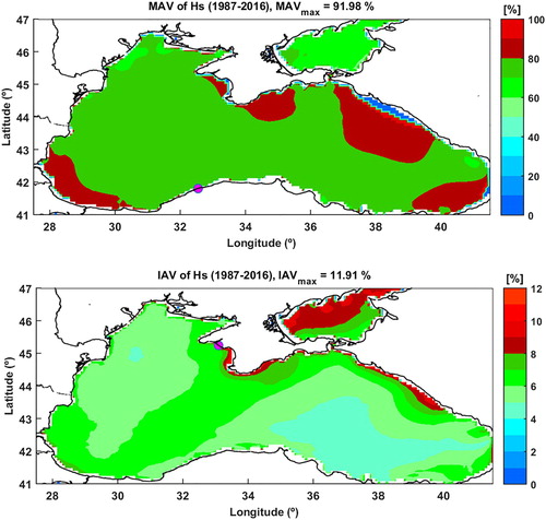
Other indexes used for climate evaluation are the mean annual variability (MAV) and inter-annual variability (IAV). The first index is the average of the annual standard deviation normalised by the annual average and it measures the spread of data, indicating also the seasonal extremes. The variability from year to year along the entire 30-year period is indicated by IAV index defined as the standard deviation of the annual means normalised by the overall mean. The relationships for both indexes are (Stopa et al. 2013):(5) $\mathrm{M}\mathrm{A}\mathrm{V}=\overline{\left(\frac{{\sigma }_k}{\overline{x_k}}\right)}$(5) (6) $\mathrm{I}\mathrm{A}\mathrm{V}=\frac{{\sigma }_{\overline{x_k}}}{\overline{x}}$(6) where the indices k refers to the year.

Figure 6 shows the MAV and IAV for significant wave heights. The MAV shows the great variability within each year over the entire basin, that is in line with the results obtained by Stopa et al. (2013) for the semi-enclosed and enclosed basins located in the Northern hemisphere. The highest values are encountered in the eastern side of the basin and near to the Bosphorus Strait. The IAV values are higher in the Azov Sea and in the north-eastern coastal environment, where the sea state conditions are more sensitive to the wind variability because in these areas the sea waves are predominant and the swell is almost not present.

Figure 6. Mean annual variability (top) and inter-annual variability for Hs.

Analysis of wave storms

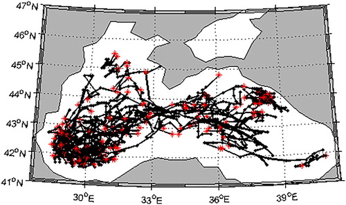
The Lagrangean methodology for wave storm identification above described was applied to significant wave height obtained from model simulation using a 5 m threshold. As extreme storm waves, only those with duration higher than 12 h were considered. For the 30-year period, a total of 151 storms were identified in the Black Sea.

In Figure 7, the location of the beginning of each identified wave storm is marked with a red star, helping to observe that wave storms do not start homogeneously through the Black Sea. Most extreme storm waves are initiated in the southwestern side of the basin, and then they will also affect the central area. In the south-eastern side, they are almost non-existent.

Figure 7. Trajectories of all storm events. Stars indicate the beginning of each storm.

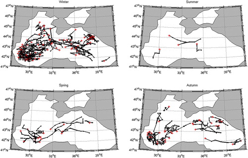
Observing the wave storm tracks in different seasons (see Figure 8), it can be seen that during winter the extreme storm waves are more frequent but also that they are more scattered. Summer is a very poor season regarding extreme storm waves as only four can be identified and they are mostly observed in central and western Black Sea. During the transition seasons, spring and autumn, some extreme storm waves can be observed. During spring wave storms are mostly generated in central and western Black Sea and move mostly eastward. During autumn, there are more extreme storm waves than during spring and they are generated mainly in southwestern and eastern Black Sea.

Figure 8. Trajectories of all storm events for each season.

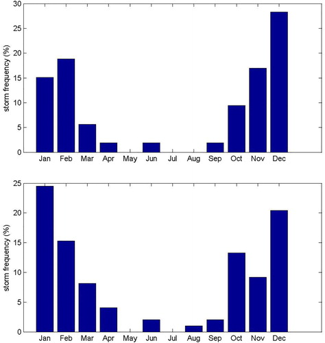
Previous studies (Rusu 2015; Divinsky and Kosyan 2017) show that the wave climate in the Black Sea has different behaviour in the western part of the Black Sea compared with the eastern part and the meridian of longitude 34°E separates the two areas. Dividing the Black Sea into two different areas, using the longitude of 34°E, the number of wave storms in each calendar month was counted and it can be seen in Figure 9 that in both regions the frequency of storms shows a seasonal distribution. The wave storms are more frequent between October and March in both regions while the stormiest month seems to be December for the eastern region, and January for the western. In the Eastern Black Sea, Autumn is the season when more wave storms develop but on the Western side, it is Winter. However, adding the wave storms that are registered in both regions, it can be seen that the winter months add almost 60% of all extreme storm events, while during the summer months the frequency of wave storms is below 10%.

Figure 9. Monthly distribution of extreme storms in Eastern side (top panel) and Western side (bottom panel) of the Black Sea.

Figure 10 shows the annual number of extreme storm waves observed in the Black Sea from 1987 to 2016. The difference between wave storms developed in the eastern and Western Black Sea can be observed by the two colours. A high inter-annual variability is present with years having between 2 and 9 wave storms. Usually, wave storms occur in both regions, but there were some years (1987, 1991, 1994, 1997 and 2012) when wave storms only developed in the western side. In average 5 wave storms are identified per year with a standard deviation of 2.19 (see Table 4). Each wave storm that is identified using the Lagrangean methodology possesses static and dynamical characteristics that can be explored. In the present work, for each wave storm, a set of characteristics were obtained and a statistical analysis of these characteristics was made and presented in Table 4.

Figure 10. Total number of storm per year during the 30 year period.

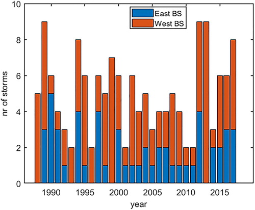
Table 4. Statistical characterisation of storm parameters.

	Mean	Max	Min	Standard deviation	Skewness	Kurtosis
Annual number of storms	5.03	9.00	2.00	2.19	0.28	2.17
Storm life time (hours)	22.29	69.00	15	9.06	2.24	9.40
Maximum Hs in storm (m)	6.88	11.80	5.20	1.12	1.53	6.51
Area of maximum Hs	46.77	266.10	1.8	42.98	2.19	9.20
Area maximum (10^3 km^2)	51.88	266.10	1.80	45.05	1.86	7.33
Length of storm track (10^3 km)	182.6	601.00	45.00	101.66	1.48	5.50

For each storm, its duration (in hours), maximum Hs observed during the storm lifetime (in meters), the area (in 10³ km²) associated to the maximum Hs, the maximum area affected by the wave storm (in 10³ km²) and the wave storm length (in 10³ Km) are evaluated and mean, maximum, minimum, standard deviation, skewness, and kurtosis are computed over all identified wave storms, in the 30 years. Some storm characteristics as maximum area, storm lifetime, maximum Hs reached during the storm event, are investigated in more detail.

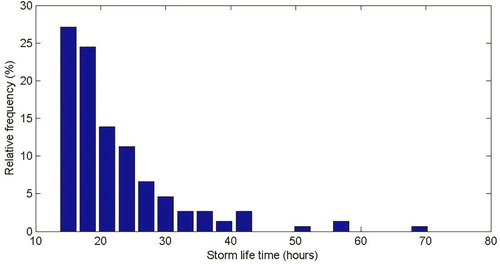
Figure 11 shows the frequency distribution of the maximum area affected by wave storm conditions. It can be observed that most storms affect an area less than 50 × 10³ km², but there are a few events that affect a much larger area, more than 250 × 10³ km². The same analysis can be made for the wave storm lifetime. Shorter storm, lasting less than a day are dominant in terms of frequency, but nevertheless, that are some extreme storm waves that lasted more than 50 h (Figure 12). There are no wave storms with less than 12 h as it is imposed in the wave storm event definition.

Figure 11. Relative frequency distribution of maximum area affected by the storm.

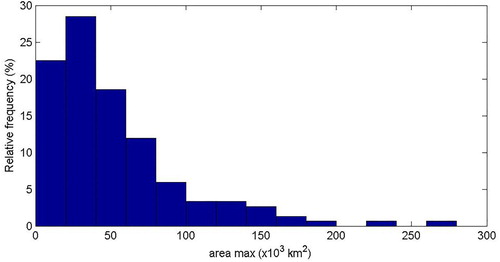
Figure 12. Relative frequency distribution of storm duration.

The frequency of the maximum value of the significant wave height in each wave storm can be observed in Figure 13. Almost 40% of the storms reach a maximum value between 6 and 7 m, but 20% reach only values between 5 and 6 m. No wave storm identified by this methodology, during this period reaches Hs higher than 12 m. In terms of the direction of the wave storm track, it can be seen in Figure 14, that, although all directions are present, more than half of the wave storm tracks are from northwest, west, and southwest, with the west being the most predominant direction.

Figure 13. Relative frequency distribution of the maximum Hs reach in each storm.

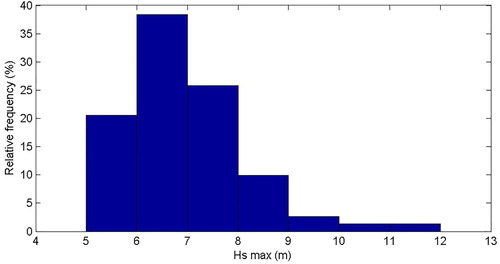
Figure 14. Relative frequency distribution of the direction of the storm trajectories.

Discussion

This study aims to evaluate the extreme storm conditions in the Black sea from 1987 to 2016, using different approaches to wave storm events, an Eulerian and a Lagrangean one. In the case of the Lagrangean approach, extreme wave storms were considered when Hs exceeded 5 m for more than 12 h. In this case, most storms can be observed in the central part of the Black Sea basin, that is also the area where storminess is expressed in terms of frequency of Hs higher than 5 m (Rusu et al. 2018a). Arkhipkin et al. (2014) also identified this region as the one where Hs reaches these higher values.

The study started with an analysis of the wave climate in seven locations. Differences between the statistical characteristics obtained for locations in distinct coastal areas can be explained by the fact that near the coast the wind is no affected only by the general circulation regimes as it is far from the coast. Due to the different types of orography, local wind regimes and breezes may be present, and together with larger scale regimes influence the wind patterns in different form (Ahrens 2012). Also, the seven locations chosen for this study although being located near the coast, they have different environmental characteristics regarding the continental shelf. Except for north-western and western areas, in general, the Black sea has a steep continental slope and a very narrow continental shelf, as it can be seen in Figure 1, and P1–P5 are located in areas less depth than P6 and P7 and this difference between deep and shallow waters can, together with different wind regimes, be determinate for the wave climate of the different locations.

Another objective of this study was to analyse trends and inter-annual variability. From the annual mean, 95th percentile and 99th percentile time series obtained for the seven locations, a strong inter-annual variability can be observed for the extremes, but not for the mean annual values, in all locations. Although linear trends were adjusted to the annual time series, and all except one location present positive values for the slope, these trends do not have statistical significance except for 95th percentile in location P1 and 99th percentile in location P2.

Valchev et al. (2012), discussed the trends in storminess in the western Black Sea and concluded that although some positive and negative trends and a complex interdecadal variability could be observed for different periods and locations, in general, no significant increase or decrease in storminess could be supported by the identified trends. Here, this conclusion is extended to other coastal areas of the Black Sea. The multidecadal variability in storminess found by Zăinescu et al. (2017), can also be observed in the oscillation of the 5-year running mean time series, of the annual extremes (Figures 3 and 4).

The evaluation of the annual frequency of extreme storm conditions in the Black Sea basin shows that it is in the southwestern part of the basin that they are more frequent. This area was also identified by Divinsky and Kosyan (2017) as the area with maximum wave energy potential. Also, Arkhipkin et al. (2014) identified it as the area where the total accumulated duration of waves higher than 4 m, during the period 1949–2010, was observed. In terms of seasonal variability, as expected, it is during Winter that extreme storm events are more frequent, followed by Spring and Autumn. During Summer, no wave storm events with Hs above 5 m were identified. This is coherent with Arkhipkin et al. (2014) that identified maximum Hs in the Black Sea, below 5 m, during the Summer and with the mean season wind magnitudes presented by Rusu (2019). This seasonal variability was also observed when Hs time series for seven locations near to the coast were analysed and the mean monthly values were computed. The strong seasonal variability with winter mean values higher than 1 m and summer reaching only about half this values. This is sustained by Valchev et al. (2012) that states that a strong seasonal variability is the most marked feature in the western Black Sea.

Large scale weather patterns over Europe, particularly influenced by the configuration of the Azores and the Siberian high pressure centres, and the Asian low pressure area, determinate the wind and wave climate in the Black Sea and its seasonal variability. In Rusu et al. (2018b), the seasonal analysis of the wind patterns of the Back Sea shows that the average wind directions change with the season, from northwest in winter, rotating to northeast during the summer, and having an intermediate direction during spring and autumn. This change in predominant wind direction also changes the fetch available for wave generation. It was observed that there are some differences in terms of the shape of the seasonal cycle and in the absolute monthly values, from some regions to the others.

The use of a Lagrangean methodology has allowed to identify wave storms as dynamical events. Observing the Figures 7 and 8, some areas are clearly more prone to extreme storm waves generation than others, and this can be explained by predominant wind direction and fetch. A relation with seasonal variability predominant wind direction and magnitude can be also made. Extreme storm events have a strong seasonal cycle, more frequent during winter, and almost non-existent during the summer. A small difference between the seasonal cycle was found for the eastern and western regions of the Black Sea.

A strong inter-annual variability is present both in the frequency of wave storms and in the different wave storm characteristics. This variability is higher than the one observed for the annual time series analysed using the Eulerian methodology. An explanation for this is that locations P1–P7 are all near the coast and the wave storm events identified with the Lagrangean methodology are located offshore, where the water depth is higher. Actually, they can be related to the areas with a higher frequency of Hs larger than 5 m, identified in Figures 5 and 6.

The statistical evaluation of the characteristics of the wave storm that was identified and that is presented in Table 4 shows a strong inter-annual variability, with values obtained for standard deviation having the same magnitude of the mean value, for characteristics related to area and length of the wave storm track. Maximum Hs and wave storm lifetime show less variability. Comparing these results with the ones obtained by Bernardino and Guedes Soares (2016) for the North Atlantic using the same methodology, but a 7 m threshold, one can see that the Black Sea is considerably less stormy. Wave storm events are less frequents, they last a shorter period and reach lower Hs values. This is, however, not surprising as the North Atlantic is considered the most energetic of the planet’s oceans (Gleizon et al. 2017) and that it covers a larger area than the Black Sea.

The shape of the statistical distribution of the maximum area affected by the wave storm, maximum Hs in storm and wave storm lifetime, are also different and further analysis should be made about the theoretical distribution that better adjust in each case.

Two storms were selected for further analysis (Figure 15). Storm A occurred during the end of January 2004 and lasted 36 h and storm B occurred during the last days of January 2006, lasting 69 h.

Figure 15. Paths of the two storms chosen for analysis.

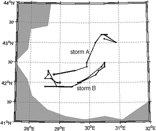
These storms have different characteristics although they were generated almost in the same area. The path of the storms can be observed in Figure 15. Storm A was also identified by Zăinescu et al. (2017) as a severe storm using both observational and modelled data at Gloria platform that is located in the western coast. Storm A starts west of 29°E and travels north-eastwards until almost the end when it slightly backs down, vanishing after 36 h.

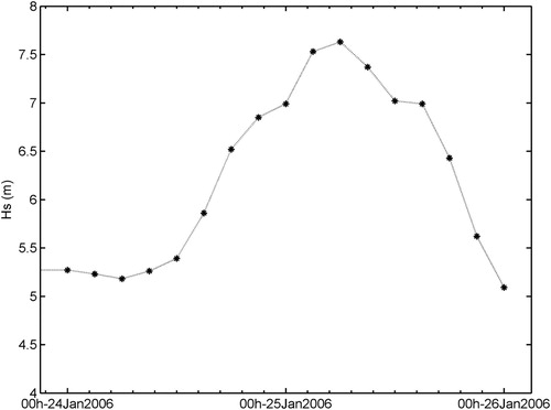
Storm B is generated in the same area but lasts much longer and travels a more complex path. First, it travels north-westwards, then turns back, travels east, and finally changes direction again and returns west. The evolution of the significant wave height during the wave storm events can be observed in Figures 16 and 17.

Figure 16. Evolution of the maximum significant wave height value in storm A.

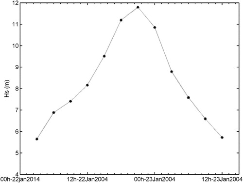
Figure 17. Evolution of the maximum significant wave height value in storm B.

Analysing the wind field for these two storm events (Figure 18 represents the average wind during the storm duration), it can be observed that during storm A, the wind magnitude (maximum of 20.05 m/s) is higher than during storm B (maximum of 17.68 m/s), but as the predominant wind is from north in the eastern side of the Black sea, the fetch is smaller than in the case of storm B. The area affected by high wind is much larger for storm A, than for storm B. This shows that although the wind is the forcing for wave generation, there are different types of wind field patterns that lead to the generation of wave storms.

Figure 18. Mean wind field obtained during the wave storm event A (left) and B (right).

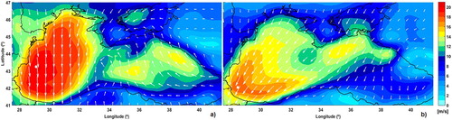
It can also be observed that the directions of the wave storm trajectories are not coincident with the predominant direction during each event. For wave storm A, the wind direction is predominant from north, but the storm moves from west to east as in wave storm B, the wind blows predominantly from northeast, but the direction of the storm path is meridional. This relation between wind direction and the direction of the wave storm should be the object of future studies. coherent with predominant wind direction.

Conclusions

This paper assesses the occurrence of extreme storm wave events in the Black Sea and their characteristics using two complementing approaches, Eulerian and Lagrangean. For the Lagrangean methodology, a 5 m threshold for significant wave height was chosen to identify extreme storm events.

The main results of this study show that extreme storm waves are seasonal, being more frequent during the winter and almost non-existent during the summer. Also, there are areas more prone to wave storm generation than others, and these areas can be related to predominant wind direction and fetch presented in Rusu (2019). The area located in the south-eastern region of the Black Sea is the one where more storms were identified, in particular, during winter (the stormiest season) and this can be associated with a region of high wind values blowing from north that was identified in the northwest side of the basin. During Autumn, the second stormiest season, the wind is weaker than during winter, but it blows from northeast enabling a larger fetch. During the other two seasons, although the fetch is similar, the wind magnitude is much lower so it is not surprising that these two seasons are less prone to wave storm events.

For the seven locations near the coast, that were chosen for this analysis, a considerable inter-annual variability was found for extreme annual values, however, for mean annual values, this variability was found to be quite low. Adjusting a linear trend to the annual values, positive values were found in almost all locations, but the statistical significance of the linear trends was only found for extreme values in two locations in the north-western coast. This means that, as it is generally the case, the climate change signal is more marked in the variability of the extremes, than in changes in mean values. Longer datasets would enable to evaluate if there are changes in the tails of the distribution of significant wave height values in this region.

The use of the Lagrangean methodology allowed to identify storm waves as dynamical events and to evaluate characteristics as storm duration, variability of the area affected by storm, maximum Hs in the storm, direction of storm trajectory, among others. Its application to the Black Sea showed that there is an inter-annual variability in all characteristics that were evaluated, more marked in the annual number of wave storms, maximum area affected by storm waves and maximum length, and less marked for maximum Hs in the storm waves and storm lifetime.

Further studies should be made using lower thresholds so that more wave storm events can be identified and a deeper analyse could be made, including a seasonal assessment of wave storm characteristics.

Acknowledgements

The authors would like to express their gratitude to the reviewers for their constructive suggestions and observations that helped in improving the present work.

Disclosure statement

No potential conflict of interest was reported by the author(s).

Additional information

Funding

This work has been performed within the project CLIMENA- CLimate change Impacts on the Marine Environment of the North Atlantic, funded by the Portuguese Foundation for Science and Technology (FCT- Fundação Portuguesa para a Ciência e a Tecnologia) [PTDC/EAM_OCE/28561/2017] and it contributes to the Strategic Research Plan of the Centre for Marine Technology and Ocean Engineering, also financed by Portuguese Foundation for Science and Technology (Fundação para a Ciência e Tecnologia-FCT). It is also funded by Unitatea Executiva pentru Finantarea Invatamantului Superior, a Cercetarii, Dezvoltarii si Inovarii (UEFISCDI), Romanian Ministry of Research and Innovation, project number PN-III-P4-ID-PCE-2016-0028, within PNCDI III.

References

- Ahrens CD. 2012. Meteorology today: an introduction to weather, climate, and the environment. California: Cengage Learning.
- Angelides DC, Veneziano D, Shyam Sunder S. 1981. Random sea and reliability of offshore foundations. J Eng Mech Div. 107:131–148. doi: 10.1061/JMCEA3.0002688
- Arkhipkin VS, Gippius FN, Koltermann KP, Surkova GV. 2014. Wind waves in the Black Sea: results of a hindcast study. Nat Hazard Earth Syst Sci. 14(11):2883. doi: 10.5194/nhess-14-2883-2014
- Bento AR, Rusu E, Martinho P, Guedes Soares C. 2014. Assessment of the changes induced by a wave energy farm in the nearshore wave conditions. Comput Geosci. 71:50–61. doi: 10.1016/j.cageo.2014.03.006
- Bernardino M, Boukhanovsky AV, Guedes Soares C. 2008. Alternative approaches to storm statistics in the ocean. Proceedings of the 27th International Conference on Offshore Mechanics and Arctic Engineering, ASME Paper OMAE2008-58053.
- Bernardino M, Guedes Soares C. 2015. A Lagrangian perspective of the 2013/2014 winter wave storms in the North Atlantic. In: Guedes Soares C., Santos T.A., editor. Maritime technology and engineering. London: Taylor & Francis Group; p. 1381–1388.
- Bernardino M, Guedes Soares C. 2016. A climatological analysis of storms in the North Atlantic. In: Guedes Soares C., Santos T.A., editor. Maritime Technology and Engineering ( Vol. 3). London: Taylor & Francis Group; p. 1021–1026.
- Booij N, Ris RC, Holthuijsen LH. 1999. A third-generation wave model for coastal regions: 1. Model description and validation. J Geophys Res. 104:7649–7666. doi: 10.1029/98JC02622
- Borgman L. 1973. Probabilities for the highest wave in a hurricane. ASCE J Waterw Harb Coast Eng. 99:185–207.
- Boukhanovsky AV, Krogstad HE, Lopatoukhin LJ, Rozhkov VA, Athanassoulis GA, Stephanakos CN. 2003. Stochastic simulation of inhomogeneous metocean fields. Part II: synoptic variability and rare events. Lect Notes Comput Sci. 2658:223–233. doi: 10.1007/3-540-44862-4_25
- Boukhanovsky AV, Lopatoukhin LJ, Ryabinin VE. 1998. Evaluation of the highest wave in a storm. Reports of World Meteorological Organization, WMO/TD. Vol. 858; 21 p.
- Butunoiu D, Rusu E. 2012. Sensitivity tests with two coastal wave models. J Environ Protect Ecol. 13(3):1332–1349.
- Campos R, Guedes Soares C. 2016. Comparison and assessment of three wave hindcasts in the North Atlantic Ocean. J Oper Oceanogr. 9(1):26–44.
- Cherneva Z, Andreeva N, Pilar P, Valchev N, Petrova PG, Guedes Soares C. 2008. Validation of the WAMC4 wave model for the Black Sea. Coast Eng. 55(11):881–893. doi: 10.1016/j.coastaleng.2008.02.028
- Davies G, Callaghan DP, Gravois U, Jiang W, Hanslow D, Nichol S, Baldock T. 2017. Improved treatment of non-stationary conditions and uncertainties in probabilistic models of storm wave climate. Coast Eng. 127:1–19. doi: 10.1016/j.coastaleng.2017.06.005
- Divinsky BV, Kosyan RD. 2017. Spatiotemporal variability of the Black Sea wave climate in the last 37 years. Cont Shelf Res. 136:1–19. doi: 10.1016/j.csr.2017.01.008
- Dupuis H, Michel D, Sottolichio A. 2006. Wave climate evolution in the Bay of Biscay over two decades. J Mar Syst. 63(3):105–114. doi: 10.1016/j.jmarsys.2006.05.009
- Galabov V, Chervenkov H. 2018. Study of the Western Black Sea storms with a focus on the storms caused by cyclones of North African origin. Pure Appl Geophys. 175:3779–3799. doi: 10.1007/s00024-018-1844-7
- Gleizon P, Campuzano F, Carracedo P, Martinez A, Goggins J, Atan R, Nash S. 2017. Wave energy resources along the European Atlantic coast. In: Yang Z., Copping A., editor. Marine renewable energy. Cham: Springer; p. 37–69.
- Graham C. 1982. The parameterization and prediction of wave height and wind speed persistence statistics for oil industry operational planning purposes. Coast Eng. 6:303–329. doi: 10.1016/0378-3839(82)90005-9
- Guedes Soares C. 2008. Hindcast of dynamic processes of the ocean and coastal areas of Europe. Coast Eng. 55(11):825–826. doi: 10.1016/j.coastaleng.2008.02.007
- Guedes Soares C, Cherneva Z, Antao E. 2004. Steepness and asymmetry of the largest waves in storm sea states. Ocean Eng. 31:1147–1167. doi: 10.1016/j.oceaneng.2003.10.014
- Haring RE, Osborne AR, Spencer LP. 1976. Extreme wave parameters based on continental shelf storm wave records. Coast Eng Proc. 1:15. doi: 10.9753/icce.v15.15
- Ivan A, Gasparotti C, Rusu E. 2012. Influence of the interactions between waves and currents on the navigation at the entrance of the Danube delta. J Environ Protect Ecol. 13(3A):1673–1682.
- Jardine TP, Latham FR. 1981. An analysis of wave heights records for the NE Atlantic. Q J Roy Met Soc. 107:415–426. doi: 10.1002/qj.49710745211
- Kislov AV, Surkova GV, Arkhipkin VS. 2016. Occurrence frequency of storm wind waves in the Baltic, Black, and Caspian seas under changing climate conditions. Russ Meteorol Hydrol. 41(2):121–129. doi: 10.3103/S1068373916020060
- Laface V, Arena F. 2016. A new equivalent exponential storm model for long-term statistics of ocean waves. Coast Eng. 116:133–151. doi: 10.1016/j.coastaleng.2016.06.011
- Laface V, Arena F, Guedes Soares C. 2015. Directional analysis of sea storms. Ocean Eng. 107:45–53. doi: 10.1016/j.oceaneng.2015.07.027
- Laugel A, Menendez M, Benoit M, Mattarolo G, Méndez F. 2014. Wave climate projections along the French coastline: dynamical versus statistical downscaling methods. Ocean Model. 84:35–50. doi: 10.1016/j.ocemod.2014.09.002
- Li F, van Gelder PHAJM, Ranasinghe R, Callaghan DP, Jongejan RB. 2014. Probabilistic modelling of extreme storms along the Dutch coast. Coast Eng. 86:1–13. doi: 10.1016/j.coastaleng.2013.12.009
- Lopatoukhin L, Boukhanovsky A, Chernysheva E. 2013. Spatial storm statistics. In EGU General Assembly Conference Abstracts (Vol. 15).
- Lucas C, Muraleedharan G, Guedes Soares C. 2017. Regional frequency analysis of extreme waves in a coastal area. Coast Eng. 126:81–95. doi: 10.1016/j.coastaleng.2017.06.002
- Mathiesen M. 1994. Estimation of wave height duration statistics. Coast Eng. 23:167–181. doi: 10.1016/0378-3839(94)90021-3
- Menendez M, Mendez FJ, Izaguirre C, Luceno A, Losada IJ. 2009. The influence of seasonality on estimating return values of significant wave height. Coast Eng. 56(3):211–219. doi: 10.1016/j.coastaleng.2008.07.004
- Onea F, Rusu L. 2017. A long-term assessment of the Black Sea wave climate. Sustainability. 9(10):1875. doi: 10.3390/su9101875
- Petruaskas C, Aagaard PM. 1971. Extrapolation of historical storm data for estimating design wave heights. J Soc Pet Eng. 11:23–37. doi: 10.2118/3127-PA
- Rusu E, Guedes Soares C. 2012. Modeling waves in open coastal areas and harbors with phase-resolving and phase-averaged models. J Coast Res. 29(6):1309–1325. doi: 10.2112/JCOASTRES-D-11-00209.1
- Rusu L. 2015. Assessment of the wave energy in the Black Sea based on a 15-year hindcast with data assimilation. Energies. 8(9):10370–10388. doi: 10.3390/en80910370
- Rusu L. 2019. The wave and wind power potential in the western Black Sea. Renew Energy. 139:1146–1158. doi: 10.1016/j.renene.2019.03.017
- Rusu L, Bernardino M, Guedes Soares C. 2014a. Wind and wave modelling in the Black Sea. J Oper Oceanogr. 7(1):5–20.
- Rusu L, Bernardino M, Guedes Soares C. 2018a. Analysis of extreme storms in the Black Sea. In: Guedes Soares C., Santos T.A., editor. Progress in maritime engineering and technology. London: Taylor and Francis Group; p. 699–704.
- Rusu L, Butunoiu D, Rusu E. 2014b. Analysis of the extreme storm events in the Black Sea considering the results of a ten-year wave hindcast. J Environ Protect Ecol. 15(2):445–454.
- Rusu L, Ganea D, Mereuta E. 2018b. A joint evaluation of wave and wind energy resources in the Black Sea based on 20-year hindcast information. Energy Explor Exploit. 36(2):335–351. doi: 10.1177/0144598717736389
- Saha S, Moorthi S, Wu X, et al. 2014. The NCEP climate forecast system version 2. J Clim. 27(6):2185–2208. doi: 10.1175/JCLI-D-12-00823.1
- Stopa JE, Cheung KF, Tolman HL, Chawla A. 2013. Patterns and cycles in the climate forecast system reanalysis wind and wave data. Ocean Model. 70:207–220. doi: 10.1016/j.ocemod.2012.10.005
- Trifonova EV, Valchev NN, Andreeva NK, Eftimova PT. 2012. Critical storm thresholds for morphological changes in the western Black Sea coastal zone. Geomorphology. 143:81–94. doi: 10.1016/j.geomorph.2011.07.036
- Trigo IF. 2006. Climatology and interannual variability of storm-tracks in the Euro-Atlantic sector: a comparison between ERA-40 and NCEP/NCAR reanalyses. Clim Dyn. 26(2-3):127–143. doi: 10.1007/s00382-005-0065-9
- Valchev NN, Trifonova EV, Andreeva NK. 2012. Past and recent trends in the western Black Sea storminess. Nat Hazard Earth Syst Sci. 12(4):961–977. doi: 10.5194/nhess-12-961-2012
- Vettor R, Guedes Soares C. 2015. Detection and analysis of the main routes of voluntary observing ships in the North Atlantic. J Navig. 68:397–410. doi: 10.1017/S0373463314000757
- Vettor R, Guedes Soares C. 2016. Rough weather avoidance effect on the wave climate experienced by oceangoing vessels. Appl Ocean Res. 59:606–6015. doi: 10.1016/j.apor.2016.06.004
- Zăinescu FI, Tătui F, Valchev NN, Vespremeanu-Stroe A. 2017. Storm climate on the Danube delta coast: evidence of recent storminess change and links with large-scale teleconnection patterns. Nat Hazards. 87(2):599–621. doi: 10.1007/s11069-017-2783-9