Evaluating wind datasets for wave hindcasting in the NW Iberian Peninsula coast

ABSTRACT

The available wind datasets can be exploited to support the setup of accurate wave models, able to reproduce and forecast extreme event scenarios. It is of utmost importance in the actual context of climate change. This study focuses on evaluating the performance of a numerical wave model, using different wind datasets, helping to create a tool to assess coastal risks, and further on to support the future implementation of reliable warning systems based on numerical models. The numerical model SWAN was implemented, configured and validated for the NW Iberian Peninsula coast, as a test case region. A period of two months, from December 2013 to January 2014, was simulated due to the winter storms that crossed the area. Six distinct wind datasets were selected to test their suitability in regional wave modelling. The results were validated against several sets of wave buoy data, considering wave parameters such as significant wave height, mean wave period and peak direction. The implemented wave model configuration allowed the representation of the wave evolution with relatively good accuracy. All the wind datasets were able to produce reasonably good wave condition estimates. The dataset that best represented the wave properties varied from one wave parameter to another, but the most reliable for the selected region was the reanalysis product generated at the European Centre for Medium-Range Weather Forecasts.

KEYWORDS:

• Wave activity
• SWAN
• coastal processes
• wind datasets comparison
• NW Iberian Peninsula coast

1. Introduction

The wave action in coastal zones can generate strong erosion. During extreme events, the combination of wave setup and hazardous wave conditions may result in significant risks to coastal navigation, structures, ecosystems and population. To minimise the risks on a vulnerable coastline, it is necessary to anticipate the storm's impacts and increase the coastal resilience. The Intergovernmental Panel on Climate Change (IPCC) depicts a future with an increase in the frequency and strength of the extreme events and larger waves, associated with sea-level rise (IPCC 2014). Monitoring the ocean condition is needed to describe the coastal dynamics. However, they are vast, and thus, the observational data is scattered over large areas (Bastos et al. 2016). Numerical models can fill this gap, being able to represent the complex patterns of coastal dynamics and allow to set up early warning tools to predict the potential effects of storms on coastal environments.

The growing importance of accurate prediction of wave conditions and wave climate requires continuous improvements of the modelling systems. The model's performance depends both on a correct physical formulation and on the quality of the forcing wind data. The accuracy of the wind products can change from one region to another and should be taken into account when choosing the best dataset to force a wave model. Àlvarez et al. (2014) evaluated different wind products for the Bay of Biscay through comparisons with real data. Carvalho et al. (2013) tested QuikSCAT and Cross-Calibrated Multi-Platform (CCMP) project wind datasets for the Iberian Peninsula. QuikSCAT products were also validated for the Ligurian Sea by Pensieri et al. (2010), while Sharp et al. (2015) assessed the UK CFSR hourly wind speed product using onshore and offshore wind measurements.

Regarding the datasets efficiency in ocean modelling, Stopa and Cheung (2014) carried out a long-term (1980–2010) inter-comparison of wind speed and wave height from ERA-Interim and CFSR in the NE Pacific and NW Atlantic. Both products have good spatial homogeneity, with a consistent level of errors, and show that ERA-Interim generally underestimates and CFSR tends to over-predict the wind speed and wave heights. Appendini et al. (2013) assessed the wave modelling performance in the Gulf of Mexico and Western Caribbean Sea, analysing NCEP/National Centre for Atmospheric Research (NCAR), ERA-Interim and NCEP's North American Regional Reanalysis (NARR) wind products. They found that NCEP/NCAR and ERA-Interim data sets outperform NARR. NARR is more suitable for simulating extreme cyclonic events due to its higher-resolution in time and space. However, the capabilities of different wind datasets for wave modelling forecasting in the Iberian Peninsula has so far received little attention.

For this study, the numerical wave model SWAN was selected. It has been successfully applied to several oceans and seas (Lalbeharry and Ritchie 2009; Van der Westhuysen 2012; Alari 2013; Viitak et al. 2016), and also to the Iberian Peninsula coast, assessing the performance of its numerical and physical formulations (Faria 2009; Rusu and Soares 2013; Rusu et al. 2015; Silva et al. 2015).

The goal of this work is to implement and validate SWAN v41.10 (SWAN 2016), using six wind data products and applying them to the NW Coast of the Iberian Peninsula (NWCIP). The following questions will be addressed. Which wind dataset leads to the most accurate simulation of wave propagation? How do the spatial and temporal properties of wind data influence wave modelling? How accurate is the SWAN wave model? This paper is structured as follows: in section 2, the materials and methods used are introduced. Section 3, presents the results and section 4 the discussion. Conclusions are summed up in section 5.

2. Materials and methods

2.1. Characterisation of the study area

The NWCIP is a complex region in terms of meteo-oceanic conditions (Bastos et al. 2016). It is characterised by a relatively narrow continental shelf (<40 km-wide) and a steep continental slope (>20°). The ocean becomes deeper than 1000 m in just a few tens of kilometres away from the coast (Gómez-Gesteira et al. 2011). The coastal bathymetry presents prominent capes, submarine canyons and promontories that induce hydrodynamic features such as filaments and eddies (Pinheiro et al. 1996; Peliz et al. 2003; Lavín et al. 2006; Mason et al. 2006; Relvas et al. 2007; Rossi et al. 2013).

The North Atlantic Oscillation (NAO), mainly mediate the weather conditions in the NWCIP. The Azores High induces northerly and north-westerly (NW) winds over the area that are prevalent throughout the year, with the highest magnitudes in the summer season (Ramos et al. 2011). As a result, dominant NW waves are produced with a mean Hs of 2m and a peak period between 9 and 13s (Costa and Esteves 2008). During winter, low-pressure systems generated over the Atlantic can cross the NWCIP with associated south-westerly (SW) and south (S) winds, producing extremely high energetic conditions on the continental shelf (Vitorino et al. 2002a). Hs between 3 and 6m are not uncommon, reaching between 9 and 12m during strong storm events (Dias et al. 2002; Vitorino et al. 2002a, 2002b; Costa and Esteves 2008).

2.2. Case study: winter storm events

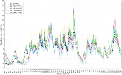
The time window between 12/2013 and 01/2014 was selected, because during this period, several storms hit the NWCIP causing extensive damage to infrastructures, such as roads and harbours (Rusu et al. 2015). Between 5-7/01/2014, the passage of the low-pressure system Hercules caused floods in coastal areas, washed away sand dunes and dragged away breakwater concrete armour units, leaving behind considerable damage in harbours, beach structures, roads, sidewalks and promenades. Deposits of sand, mud and debris were moved inland (Santos et al. 2014). During this event, strong SW winds blew over the entire region, producing long period waves with measured maximum wave heights between 7 and 12 m (Figure 1). During the entire analysis period, the mean wave direction was from the N–W sector, with mean Hs between 4 and 5 m, mean wave period from 7 to 9s.

Figure 1. Hs evolution observed for the 6 buoys during the study period (01/12/2013–31/01/2014).

2.3. Wind data products

Surface wind fields were obtained from six databases (Table 1), with a reference height of 10 m above the sea level. They were applied in different stages depending on their spatial coverage.

Table 1. Wind datasets characteristics.

Dataset	$\mathrm{\Delta }x\times \mathrm{\Delta }y$ (^o)	$\mathrm{\Delta }t$ (h)	Availability
ECMWF Era-Interim	$0.75\times 0.75$	6	1979–2019
ECMWF ERA5	$0.2815\times 0.2815$	1	2010–present
NASA MERRA-2	$0.5\times 0.625$	1	1980–present
NCEP CFSv2 (ds094.0)	$0.5\times 0.5$	1	2011–present
NCEP CFSv2 (ds094.1)	$0.5\times 0.5$	1	2011–present
WRF-MeteoGalicia	$0.1079\times 0.1079$	1	2008–present

From the ECMWF, the two most recent reanalysis were selected: ERA-Interim (Dee et al. 2011) and ERA5 (Copernicus Climate Change Service 2017). ERA-Interim is a global atmosphere reanalysis, continuously updated in real-time with data available since 1979. ERA5 is a recent reanalysis of the EU-funded Copernicus Climate Change Service (C3S) operated by ECMWF. The first segment (2010–2016) provides data at higher spatial and temporal resolution than ERA-Interim.

MERRA-2 (GMAO 2015), the second version of NASA atmospheric reanalysis was constructed using the Goddard Earth Observing System Model V5 with Atmospheric Data Assimilation System.

From the NCEP products, the 6-hourly forecast surface winds products from CFSv2 ds094.0 and the hourly time-series from CFSv2 ds094.1 were selected (Saha et al. 2011a, 2011b and 2014).

Finally, historical forecasts from the regional Weather Research and Forecasting model, implemented by MeteoGalicia (http://www.meteogalicia.gal/) for local forecast, were considered. This model runs operationally twice a day with three available domains and spatial resolutions. The highest spatial resolution product was selected.

2.4. Observational data

Model results were validated against data from six wave-buoys at various depths (Figure 2(b)). Leixões (P1) is maintained by the Instituto Hidrográfico (IH, http://www.hidrografico.pt/boias-ondografo.php). The directional Waverider Datawell is moored in shallow waters (83 m), and records data in a 3-hours interval, increasing the frequency during energetic events (Hs > 5 m). Cabo Silleiro (P2), Villano-Sisargas (P3), Estaca de Bares (P4), Cabo de Peñas (P5) and Bilbao-Vizcaya (P6) are maintained by Puertos del Estado (http://www.puertos.es/), gathering data in a 1-hour interval. They are equipped with a directional Met-Oce sensor and located in relatively deep waters close to the continental shelf border or areas of complex bathymetry and strong depth gradients.

Due to the resolution of the available bathymetric data and the discrete nature of the computational grids, there is a difference between the computed depth and the real depth at the buoy locations (Table 2), especially evident for the coarser grid.

Table 2. Buoys location and depth (real and interpolated at the numerical grids).

Buoy	Name	Location		Depth (m)
		Latitude	Longitude	Real	G1	G2	G3
P1	Leixões	41.32 ^oN	8.98 ^oW	83	84	82	86
P2	Cabo Silleiro	42.12 ^oN	9.43 ^oW	600	2564	702	700
P3	Villano-Sisargas	43.50 ^oN	9.21 ^oW	386	Inland	422	482
P4	Estaca de Bares	44.12 ^oN	7.67 ^oW	1800	751	1514	1586
P5	Cabo de Peñas	43.75 ^oN	6.16 ^oW	615	2393	350	497
P6	Bilbao-Vizcaya	43.64 ^oN	3.09 ^oW	870	1789	894	Outside

2.5. Numerical model setup

SWAN is a third-generation wave model developed at the Delft University of Technology. Short-crested wind-wave generation and propagation over realistic bathymetry are described by means of a two-dimensional wave action density spectrum. A spectral wave action balance equation is solved without any a priori restrictions on the spectrum for wave growth evolution (Booij et al. 1999).

A grid nesting procedure was implemented to guarantee proper simulation of nearshore processes. Three computational grids with different spatial extent and resolution were defined (Figure 2(a)). The first and coarser grid, G1 (1°x1°), covered the whole North Atlantic to provide swell information for inner computational grids (G2, G3). It lacks detailed information on depth over the continental slope and shelf, thus significantly altering the nearshore wave processes and leading to inaccurate readings at buoys locations. Nevertheless, G1 resolution was enough to accurately represent the long-wavelength low-frequency waves travelling across the ocean. The first nested level or second grid G2 (7.5’×7.5’), covered most of the oceanic area around the Iberian Peninsula. Finally, the second nested level G3 (28.125’’×28.125’’) covered the NW coastal seas of the Iberian Peninsula. The increase in the resolution along with the reduction of the observed area (Figure 2(a)) allowed a better agreement between the buoys real depth and depth on the grid (Table 2).

Figure 2. a) Nesting set-up and computational grids G1, G2 and G3 placements and b) bathymetry of the G2 computational area. The two sectors of the study area are, Atlantic (West) and Cantabrian (North), marked with black intermediate lines and the red isoline indicates the border of the continental shelf. Additionally, the locations of wave buoys are shown with yellow squares.

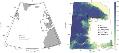
Bathymetric information for G1 was extracted from the GEBCO 30’’ global grid (Becker et al. 2009). G2 and G3, used information extracted from the West Iberian bathymetry model WIBM2009 (Quaresma and Pichon 2013), which has 1’ resolution.

G1 results were compared with observational data from five wave-buoys (P1, P2, P4, P5, P6) out of six. P3 was considered as a land cell on this grid due to the low resolution, as each cell covered an area of, approximately, 112 × 112 km, causing some inaccuracies in the coastal line representation. G3 covered also five buoys out of six (P1, P2, P3, P4, P5), leaving out the most eastward wave buoy (P6) (cf. Figure 2(b)).

In the G1 level all the wind datasets except MeteoGalicia, due to its limited spatial coverage, were used for the wave hindcast. For the next nesting level G2, MeteoGalicia data plus the three G1 best performing wind datasets were applied. The boundary conditions for the simulation with MeteoGalicia winds were obtained from the G1 grid run with ERA5 wind data. In the second nesting level G3, the three best performing wind datasets in G2 were tested.

A spin-up time of 1 week was considered to avoid model inconsistencies. After several tests, spectral directional resolution of 5° and 25 spectral frequency bins logarithmically spaced between 0.0418 and 0.8 Hz were chosen. For G1 and G2 the higher-order numerical S&L scheme and Janssen whitecapping formulation (Janssen 1991) were selected. At G3, the first-order upwind scheme BSBT was applied to guarantee the numerical stability (SWAN 2013) and Westhuysen whitecapping (Van der Westhuysen et al. 2007) was chosen.

2.6. Validation method

To assess the quality of the results, a statistical analysis was performed for three wave parameters: significant wave height (Hs) and the spectrum mean zero-up-crossing wave period (Tm02), calculated from the density spectrum as:(1) $Hs=4\sqrt{\int \int E\left(\omega ,\theta \right)d\omega d\theta }$(1) (2) $Tm02=2\pi {\left(\frac{\int \int {\omega }^{2}E\left(\omega ,\theta \right)d\omega d\theta }{\int \int E\left(\omega ,\theta \right)d\omega d\theta }\right)}^{-{\displaystyle \frac{1}{2}}}=2\pi {\left(\frac{\int \int {\omega }^{2}E\left(\sigma ,\theta \right)d\sigma d\theta }{\int \int E\left(\sigma ,\theta \right)d\sigma d\theta }\right)}^{-{\displaystyle \frac{1}{2}}}$(2)

and, the spectrum peak wave direction (Pdir), which is the peak direction in E(θ) = ∫E(ω,θ)dω, where E is the variance density spectrum, ω the absolute circular frequency determined by the Doppler shifted dispersion and θ the wave propagations direction. Note that Pdir, correspond to the absolute maximum bin of the corresponding discrete wave spectra E(θ) hence might not be the real Pdir.

Four statistical parameters, the Root Mean Square Error (RMSE), the Scatter Index (SI), the mean error (BIAS), and the correlation coefficient (Cor) were considered:(3) $RMSE=\sqrt{\frac{1}{n}\sum _{i=1}^n{\left(a_i-b_i\right)}^2}$(3) (4) $SI=\frac{RMSE}{{\displaystyle \frac{1}{n}{\sum }_{i=1}^n{b}_i}}\times 100$(4) (5) $BIAS=\frac{{\sum }_{i=1}^n\left(a_i-b_i\right)}{n}$(5) (6) $Cor\left(a,b\right)=\frac{coc\left(a,b\right)}{{\sigma }_a{\sigma }_b}$(6)

where a represents the model results, b the observed measurements, n the number of observations, cov(a,b) the covariance between a and b, and σ_a and σ_b the standard deviation of a and b, respectively.

Regarding Pdir, to eliminate any discontinuity between 0° and 360°, the difference between observations θ_obs and model results θ_mod was obtained (Pensieri et al. 2010). The corrected values were calculated as:(7) ${\theta }_{mod}={\theta }_{mod}-{360}^{\circ }when{\theta }_{obs}-{\theta }_{mod}>{180}^{\circ }$(7)

(8) ${\theta }_{mod}={\theta }_{mod}+{360}^{\circ }when{\theta }_{obs}-{\theta }_{mod}<=-{180}^{\circ }$(8)

However, and due to the proper definition of the statistical parameters, SI was not calculated for Pdir, and the results of this variable were validated using only RMSE.

3. Results

3.1. Wind datasets performance

3.1.1. Significant wave height (Hs)

The results show a good performance for all the considered wind datasets, with a satisfactory reproduction of the Hs evolution over time. Nevertheless, some differences arise in terms of Hs magnitude. ECMWF products and MERRA-2 were underestimating the highest Hs peaks, while the NOAA-NCEP datasets were largely overestimating. Both ECMWF products gave similar results, but some improvements can be seen with ERA5 (Figure 3(a)).

Figure 3. Measured and modelled Hs for the period between 01.12.13–31.01.14. Red dots represent buoys measurement, dotted lines are SWAN results for each wind dataset considered. The bold line indicates the best fit for each buoy. a) Comparison of measurements and G1 computational grid. b) Measured and modelled results with ERA5 wind data, representing all three computational grids in buoy locations P2 and P5.

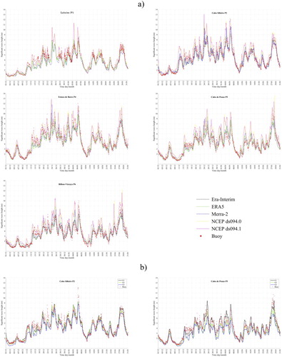
The best wind dataset for Hs at G1 was ERA5 (Table 3.a), giving the best results for three considered buoys (P1, P4, P5). In these locations, ERA5, RMSE varies from 0.43–0.71 m, SI from 9.30–17.52%, BIAS from −0.12–0.17 m and Cor from 0.92–0.95. For P2 and P6, the best results are obtained with MERRA-2 and ERA-Interim, respectively.

Table 3. RMSE, SI, BIAS and Cor for each computational domain (G1, G2 and G3) at buoys location for a) significant wave height, b) mean wave period and c) wave peak direction. The most optimal dataset for each domain is marked in bold.

	Mean (m)			RMSE (m)			SI (%)			BIAS			Cor
a) Hs	G1	G2	G3	G1	G2	G3	G1	G2	G3	G1	G2	G3	G1	G2	G3
P1	4.62
ERA-Interim	4.17	4.24	4.04	0.47	0.44	4.48	10.12	9.46	10.47	-1.18	-0.15	-0.22	0.92	0.92	0.94
ERA5	4.30	4.36	4.12	0.43	0.40	0.45	9.30	8.74	9.76	-0.12	-0.10	-0.19	0.92	0.92	0.94
Merra-2	4.09			0.55			11.98			-0.21			0.89
NCEP CFSv2 (ds094.0)	5.10	5.13		0.62	0.62		13.52	13.45		0.18	0.20		0.89	0.89
NCEP CFSv2 (ds094.1)	5.08			0.64			13.84			0.18			0.80
MeteoGalicia WRF		4.50	4.12		0.44	0.46		9.57	9.98		-0.05	-0.19		0.90	0.93
P2	4.30
ERA-Interim	4.21	4.02	3.71	0.68	0.71	0.82	15.84	16.39	19.16	-0.10	-0.29	-0.59	0.94	0.95	0.96
ERA5	4.28	4.08	3.76	0.67	0.66	0.81	15.49	15.26	18.72	-0.02	-0.22	-0.55	0.94	0.95	0.96
Merra-2	4.29			0.64			14.85			-0.01			0.95
NCEP CFSv2 (ds094.0)	5.22	4.91		1.27	1.03		29.55	24.04		0.92	0.61		0.93	0.94
NCEP CFSv2 (ds094.1)	5.18			1.33			30.96			0.88			0.90
MeteoGalicia WRF		4.21	3.77		0.72	0.78		16.67	18.21		-0.09	-0.53		0.94	0.96
P3	4.52
ERA-Interim		4.53	4.06		0.63	0.67		13.97	14.82		0.00	-0.36		0.94	0.96
ERA5		4.41	3.99		0.55	0.71		12.25	15.67		-0.08	-0.41		0.95	0.96
NCEP CFSv2 (ds094.0)	5.36			1.08			23.77			0.64			0.94
MeteoGalicia WRF		4.66	4.07		0.76	0.67		16.73	14.77		0.11	-0.35		0.93	0.96
P4	4.57
ERA-Interim	4.30	4.32	3.82	0.77	0.75	0.99	16.77	16.43	21.65	-0.27	-0.25	-0.75	0.94	0.94	0.96
ERA5	4.31	4.31	3.82	0.71	0.72	1.01	15.57	15.77	22.14	-0.26	-0.26	-0.75	0.95	0.95	0.95
Merra-2	4.31			0.86			18.82			-0.25			0.92
NCEP CFSv2 (ds094.0)	5.31	5.24	1.14	1.09	24.85	23.96	0.74	0.67	0.94	0.94
NCEP CFSv2 (ds094.1)	5.29	1.20	26.15	0.72	0.93
MeteoGalicia WRF		4.60	3.95		0.90	0.91		19.66	19.82		0.03	-0.62		0.92	0.95
P5	3.79
ERA-Interim	3.77	3.10	2.94	0.71	0.93	1.07	18.68	24.57	28.17	-0.03	-0.70	-0.86	0.92	0.95	0.95
ERA5	3.96	3.24	3.02	0.66	0.83	1.01	17.52	22.00	26.60	0.17	-0.56	-0.77	0.94	0.94	0.95
Merra-2	3.95			0.74			19.38			0.15			0.93
NCEP CFSv2 (ds094.0)	4.86	3.86		1.43	0.64		37.60	16.86		1.07	0.06		0.93	0.94
NCEP CFSv2 (ds094.1)	4.89			1.51			39.72			1.09			0.91
MeteoGalicia WRF		3.72	3.22		0.83	0.81		21.88	21.40		-0.07	-0.57		0.91	0.95
P6	3.46
ERA-Interim	3.32	2.83		0.64	0.90		18.39	26.04		-0.14	-0.63		0.94	0.95
ERA5	3.58	3.17		0.72	0.77		20.74	22.33		0.12	-0.29		0.92	0.92
Merra-2	3.63			0.72			20.92			0.17			0.92
NCEP CFSv2 (ds094.0)	4.41	3.79	1.33	0.78	38.49	22.45	0.96	0.33	0.91	0.92
NCEP CFSv2 (ds094.1)		4.45			1.43			41.46			1.00			0.88
MeteoGalicia WRF		3.35			0.81			23.38			-0.11			0.89
	Mean (m)			RMSE (m)			SI (%)			BIAS			Cor
b) Tm02	G1	G2	G3	G1	G2	G3	G1	G2	G3	G1	G2	G3	G1	G2	G3
P1	8.94
ERA-Interim	7.62	7.86	7.90	1.24	1.13	0.85	13.85	12.56	9.55	-0.51	-0.42	-0.40	0.75	0.76	0.84
ERA5	7.66	7.86	7.95	1.25	1.14	0.82	13.96	12.77	9.13	-0.49	-0.42	-0.38	0.76	0.76	0.86
Merra-2	8.46			1.14			12.71			-0.19			0.71
NCEP CFSv2 (ds094.0)	8.87	9.16		1.02	0.89		11.43	9.96		-0.03	0.09		0.79	0.82
NCEP CFSv2 (ds094.1)	8.95			1.10			12.31			0.00			0.79
MeteoGalicia WRF		7.61	7.72		1.27	0.95		14.24	10.61		-0.52	-0.47		0.72	0.84
P2	7.73
ERA-Interim	6.95	6.85	7.23	1.59	1.68	1.04	20.52	21.68	13.40	-0.78	-0.88	-0.51	0.71	0.74	0.87
ERA5	6.94	6.81	7.27	1.43	1.65	0.94	18.47	21.36	12.19	-0.79	-0.93	-0.46	0.77	0.76	0.89
Merra-2	6.94			1.58			20.45			-0.79			0.72
NCEP CFSv2 (ds094.0)	7.86	7.85		1.43	1.53		18.46	19.82		0.12	0.12		0.78	0.79
NCEP CFSv2 (ds094.1)	7.93			1.50			19.46			0.20			0.76
MeteoGalicia WRF		6.78	7.20		1.71	1.02		22.11	13.21		-0.95	-0.53		0.71	0.87
P3	7.65
ERA-Interim		6.75	7.11		1.2	0.80		15.72	10.48		-0.68	-0.41		0.81	0.90
ERA5		6.86	7.19		1.17	0.75		15.29	9.78		-0.6	-0.35		0.81	0.91
NCEP CFSv2 (ds094.0)	7.69			1.17			15.27			0.03			0.8
MeteoGalicia WRF		6.78	7.12		1.26	0.81		16.48	10.58		-0.66	-0.40		0.77	0.90
P4	7.60
ERA-Interim	6.61	6.59	7.05	1.32	1.42	0.94	17.42	18.75	12.38	-0.99	-1.01	-0.55	0.85	0.81	0.90
ERA5	6.67	6.62	7.10	1.26	1.36	0.87	16.55	17.95	11.46	-0.93	-0.97	-0.50	0.85	0.83	0.91
Merra-2	6.76			1.24			16.30			-0.84			0.83
NCEP CFSv2 (ds094.0)	7.44	7.34		0.95	1.14		12.53	14.97		-0.15	-0.26		0.86	0.84
NCEP CFSv2 (ds094.1)	7.42			1.03			13.50			-0.18			0.84
MeteoGalicia WRF		6.53	6.97		1.44	0.97		18.87	12.77		-1.06	-0.63		0.81	0.90
P5	7.56
ERA-Interim	6.82	6.46	7.38	1.40	1.8	1.12	18.52	23.81	14.83	-0.73	-1.1	-0.17	0.80	0.69	0.82
ERA5	6.69	6.62	7.43	1.49	1.51	0.96	19.66	19.93	12.70	-0.86	-0.94	-0.12	0.78	0.8	0.87
Merra-2	6.92			1.41			18.64			-0.63			0.81
NCEP CFSv2 (ds094.0)	7.59	7.21		1.40	1.35		18.53	17.9		0.03	-0.34		0.81	0.81
NCEP CFSv2 (ds094.1)	7.61			1.54			20.32			0.06			0.78
MeteoGalicia WRF		5.95	6.75		1.97	1.24		16.12	16.39		-1.61	-0.81		0.72	0.84
P6	8.31
ERA-Interim	8.31	7.01		1.98	1.9		23.88	22.89		-1.56	-1.3		0.86	0.83
ERA5	6.50	6.07		2.24	2.69		26.99	32.32		-1.81	-2.25		0.82	0.76
Merra-2	6.47			2.37			28.51			-1.84			0.77
NCEP CFSv2 (ds094.0)	7.20	6.69		1.89	2.31		22.73	27.85		-1.11	-1.62		0.80	0.73
NCEP CFSv2 (ds094.1)	7.20			1.81			21.73			-1.11			0.83
MeteoGalicia WRF			5.83			2.93			35.3			-2.48			0.72
	Mean (m)			RMSE (m)			BIAS			Cor
c) Pdir	G1	G2	G3	G1	G2	G3	G1	G2	G3	G1	G2	G3
P1	322
ERA-Interim	322	326	325	12	9	10	0.21	1.43	1.31	0.88	0.94	0.93
ERA5	324	327	326	15	11	9	0.92	2.06	1.52	0.84	0.91	0.94
Merra-2	323			10			0.44			0.92
NCEP CFSv2 (ds094.0)	322	326		10	9		0.02	1.79		0.92	0.95
NCEP CFSv2 (ds094.1)	322			11			0.19			0.90
MeteoGalicia WRF	329	325		17	10		2.81	1.08		0.83	0.93
P2	297
ERA-Interim	302	304	303	31	24	20	5.16	7.34	5.68	0.91	0.95	0.97
ERA5	304	306	304	33	27	22	7.51	9.12	6.68	0.91	0.94	0.96
Merra-2	305			26			7.95			0.94
NCEP CFSv2 (ds094.0)	303	306		27	27		6.46	9.06		0.94	0.95
NCEP CFSv2 (ds094.1)	302			29			4.88			0.93
MeteoGalicia WRF		313	305		42	24		16	7.69		0.89	0.95
P3	293
ERA-Interim		298	296		29	25		3.94	1.82		0.94	0.95
ERA5		301	298		30	25		5.73	3.25		0.94	0.95
NCEP CFSv2 (ds094.0)		300			27			4.77			0.85
MeteoGalicia WRF		303	296		37	27		7.5	1.85		0.91	0.94
P4	313
ERA-Interim	318	317	317	31	29	25	4.84	4.35	3.62	0.89	0.9	0.92
ERA5	317	313	315	33	37	27	3.84	-0.59	2.01	0.88	0.86	0.91
Merra-2	317			31			3.80			0.89
NCEP CFSv2 (ds094.0)	316	313		35	35		2.45	-0.26		0.86	0.86
NCEP CFSv2 (ds094.1)	317			30			4.29			0.89
MeteoGalicia WRF		318	314		40	34		4.82	1.09		0.83	0.87
P5	316
ERA-Interim	328	317	320	29	29	25	11.74	0.66	3.62	0.63	0.53	0.61
ERA5	321	312	317	35	34	31	5.57	-4.18	0.81	0.54	0.46	0.49
Merra-2	324			32			8.13			0.60
NCEP CFSv2 (ds094.0)	320	311		37	31		4.21	-4.87		0.52	0.5
NCEP CFSv2 (ds094.1)	320			39			4.39			0.51
MeteoGalicia WRF		315	315		38	37		-1.14	-0.68		0.43	0.43
P6	320
ERA-Interim	327	321		19	18		6.87	0.92		0.85	0.83
ERA5	325	318		29	30		4.91	-2.68		0.75	0.71
Merra-2	326			33			5.43			0.69
NCEP CFSv2 (ds094.0)	325	318		29	25		4.09	-2.64		0.74	0.75
NCEP CFSv2 (ds094.1)	326			31			5.80			0.71
MeteoGalicia WRF		323			34			2.57			0.69

G2 was forced with MeteoGalicia WRF dataset and the three best performing wind datasets in grid G1 ERA-Interim, ERA5 and NCEP CFSv6 (ds094.0). As expected, some improvements can be seen when compared with G1 (Table 3.a). For ERA-Interim, RMSE reduced between 0.02 and 0.03 m at P1 and P4, but presents higher values, up to 0.26 m, for the rest of the buoys locations. For ERA5, Hs RMSE improves few centimetres in P1 and P2, but the error increases up to 0.17 m in rest of the buoys. NCEP CFSv6 (ds094.0) demonstrates better results compared to the G1 level. Cor coefficient maintains the same values or improves a bit for the G2 domain.

G3 did not show almost any improvement over the previous grid. Comparing the statistical metrics for the three considered domains (G1, G2, G3), G3 outputs presents the worst results, even when the MeteoGalicia highest resolution wind dataset was implemented.

Minimal differences between G1 and G2 results were depicted in the estimated values for P2 (Figure 3(b)). Furthermore, the G3 results seem to lead to a higher Hs underestimation. This is further confirmed by the P5 results, where this underestimation was even larger.

The best results for Hs at G1 and G2 were produced using ERA5, for G3 MeteoGalicia.

3.1.2. Mean wave period (Tm02)

Tm02, was reasonably well represented whatever the wind dataset used at the G1 grid. Nevertheless, ERA-Interim, ERA5 and MERRA-2 lead to underestimation of the Tm02 at all the buoy locations, whereas it was overestimated at some locations for both NOAA datasets.

For the first two weeks (01/12–13/12), the mean period was largely underestimated for all the datasets with the exception for buoy P4, where SWAN results were closer to measured values than at any other considered buoy (Figure 4(a)). The correlation results reveal a better performance of the wind datasets at the Cantabrian sector, with Cor between 0.77 and 0.86. At the West Atlantic sector, Cor was lower, between 0.71 and 0.79. When compared with Hs Cor values, a decrease in the correlation of 17% in the West Atlantic sector and 11% in the Cantabrian sector was noticed (Table 3.a and b).

Figure 4. Measured and modelled Tm02 for the period between 01.12.13–31.01.14. Red dots represent buoys measurement, dotted lines are SWAN results for each wind dataset considered. The bold line indicates the best fit for each buoy. a) Comparison of measurements and G1 computational grid. b) Measured and modelled results with ERA5 wind data representing all three computational grids, in buoy locations P2 and P5.

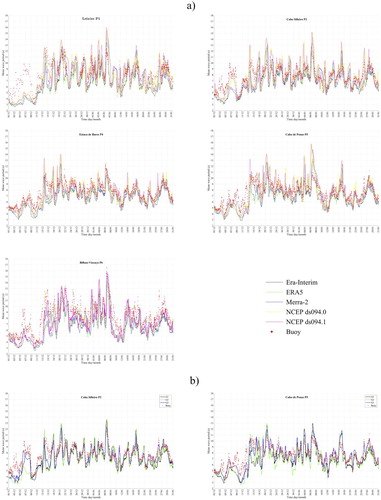
Nevertheless, and contrary to the Hs results, Tm02 for G2 presents a slightly poorer outcome at all buoys but P1, being quite improved for G3. G3 shows the best results from the three considered computational grids. RMSE for Tm02 was close to or over 1.50 s for most buoys and wind datasets for G1 and G2, while for G3 it remains below 1.0 s for ERA5 and close to 1.0 s for all the other wind datasets (Table 3.b).

For the two initial simulation weeks, G1 and G2 solutions do not accurately represent Tm02 evolution. Such pattern was corrected for the highest resolution simulation on grid G3. At P1, and after the first two weeks within the simulation, it seems that for G1 and G2, the wave energy was more spread along the frequency bins, nevertheless, the lower frequency bins were under-represented in G3. At P5, G3 results clearly show a much better performance, with a good capture of Tm02, which might indicate a better representation of the wave energy along the different frequency bins (Figure 4(b)). The best results for Tm02 at G1 and G2 were produced using NOAA NCEP ds094.0. For the three wind datasets selected for forcing the waves on G3, ERA5 led to the best results for Tm02.

3.1.3. Peak direction (Pdir)

For Pdir, the best G1 results were obtained with NCEP ds09.1, MERRA-2 and Era-Interim (Figure 5). The best statistical parameters were obtained at P1, where NCEP ds09.1 and MERRA-2 provided similar outcomes. For both datasets, RMSE was 10° and Cor was 0.92. For the other buoys, the RMSE was mostly close to 30° reaching up to 39°, with the exception of the ERA-Interim results at P6 where RMSE of 19° was obtained. All the wind datasets clearly display a bias in the peak wave direction, with a tendency for an anti-clockwise error in the estimated wave direction (Table 3.c).

Figure 5. Difference between buoys and model outcome (buoy-SWAN, G1 computational domain) with three wind datasets, ERA-Interim, Merra-2 and NCEP ds094.0.

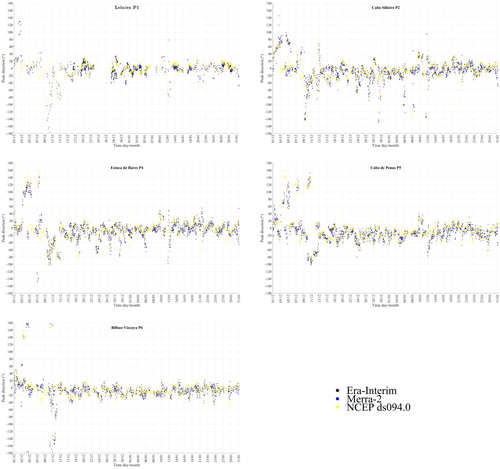
Similar to Tm02, the numerical model seems to be less accurate in estimating Pdir for all the buoys locations for the initial two weeks period.

For G2, the best wind datasets were NCEP CFSv2 (ds094.0) for P1 and P3 and Era-Interim for P2, P4, P5 and P6. For G3, the best dataset was ERA-Interim, although the Atlantic sector results present small differences (from 1° up to 4°) between the considered datasets. In the Cantabrian sector, larger differences arise, reaching up to 13° at P1.

There existed a small but consistent improvement in almost each buoy location for all the wind datasets when G1 and G3 results were compared.

4. Discussion

The presented results revealed minor differences in model solutions when using different wind datasets. Nevertheless, for each considered wave parameter, the best ones can be clearly distinguished. ERA5 gives the best results for Hs, Era-Interim for Pdir and NCEP CFSv2 (ds094.0) for Tm02, although the difference between NCEP CFSv2 (ds094.0) and ERA5 was relatively small and both can be considered to properly simulate mean wave period (Table 3.b).

The temporal and spatial characteristics of the wind datasets did not have a big influence on the results. The best Pdir results were obtained with Era-Interim, which was the lower temporal and spatial resolution database (Table 1). Therefore, to simulate the approaching swell, coarse grids and larger time steps with a proper representation of wind speed and direction, seem to be appropriate to produce accurate solutions.

The different responses observed for the wave parameters in G3 could be related to the wave spectrum. When calculating the wave variables, different parts of the wave energy spectra are considered. Hs is calculated taking into account the total wave energy, whereas the rest of the parameters are found through circular frequency or direction. Errors in the velocity and direction fields of the wind could be transferred to the wave model and may produce inaccurate frequencies transference to the surface waters. This seems not to have such a big effect on the total energy rather affecting the individual components.

Àlvarez et al. (2014) concluded that coarser databases are less reliable in near-shore areas. Additionally, they noted that the wind speed and direction are less accurate for low wind speed events (<4 m/s). In wave modelling it is not possible to determine which waves are induced with low wind speed, so another approach was considered. Calm and storm periods were analysed separately considering a 5 m wave height threshold. The results obtained at P1 and P5 with ERA5 for all the three modelling levels revealed that the more accurate Hs results were obtained mostly during calm conditions (Table 4). Tm02 and Pdir were better represented during storms. This confirms that, with lower wind speed, the wave simulations are less accurate and the total energy spectre of the waves is less affected by the individual parts.

Table 4. RMSE, SI, BIAS and Cor for each computational domain (G1, G2 and G3) at P1 and P5 in a storm and calm situation using ERA5 wind fields.

Hs					Tm02				Pdir
P1			P5		P1		P5		P1		P5
	storm	calm	storm	calm	storm	calm	storm	calm	storm	calm	storm	calm
G1 RMSE	0.33	0.28	0.43	0.51	0.74	1.01	0.60	1.36	7	13	12	33
SI	5.50	7.55	6.99	16.54	7.48	12.13	6.81	18 98
BIAS	-0.07	-0.06	0.04	0.13	-0.16	-0.34	-0.08	-0.78	0.04	0.88	4.62	0.96
Cor	0.72	0.90	0.73	0.91	0.72	0.70	0.67	0.73	0.65	0.87	0.45	0.56
Med. s	5.49	3.47	6.35	3.22	8.85	6.83	8.49	6.13
Med. M	5.91	3.72	6.17	3.06	9.84	8.31	8.85	7.16	329	317	315	316
G2 RMSE	0.30	0.27	0.59	0.59	0.64	0.94	0.63	1.37	5.05	10.17	7.48	32.86
SI	5.11	7.22	9.52	19.38	6.52	11.36	7.09	19.14
BIAS	-0.06	-0.04	-0.24	-0.32	-0.12	-0.29	-0.17	-0.77	0.58	1.48	2.25	-6.44
Cor	0.73	0.91	0.82	0.90	0.71	0.71	0.70	0.76	0.69	0.93	0.57	0.48
Med. s	5.54	3.52	5.17	2.64	9.05	7.02	8.13	6.15
Med. m	5.91	3.72	6.17	3.06	9.64	8.31	8.85	7.16	329	317	315	316
G3 RMSE	0.34	0.30	0.75	0.67	0.47	0.67	0.36	0.89	2.81	8.49	8.66	29.51
SI	5.74	7.99	12.21	21.96	4.73	8.06	4.03	12.44
BIAS	-0.11	-0.09	-0.33	-0.45	-0.15	-0.23	0.04	-0.16	0.42	1.09	3.13	-2.32
Cor	0.78	0.92	0.81	0.92	0.82	0.81	0.84	0.84	0.84	0.95	0.59	0.51
Med. s	5.24	3.34	4.79	2.47	8.90	7.29	9.00	6.95
Med. m	5.91	3.72	6.17	3.06	9.84	8.31	8.85	7.16	329	317	315	316

Our model configuration was reliable when compared with similar studies, presenting results with the same level of accuracy, or better than previously developed works (Table 5). This comparison is not straightforward due to differences such as the geographical area, the grids resolution, the location of the buoys, the type of wind data, etc. Nevertheless, it provides an indication of the type of accuracy and credibility of the wave model set-up that was implemented in this study.

Table 5. Validation results of wave mode SWAN from various studies around the world.

Author	Rusu et al. (2015)	Rusu and Soares (2013)	Silva et al. (2015)	Viitak et al. (2016)	This study
Area	West Iber. co.	Cont. Portugal	Spanish co.	Baltic Sea	NW Iber. co.
Wind	HIPOCAS	MM5	ERA-Interim	HIRLAM	ERA5
Significant wave height (Hs)
RMSE	0.74	0.40	0.81	0.28	0.45
SI	0.17	0.19	0.42	0.22	0.10
BIAS	0.23	0.12	0.36	0.19	−0.19
Cor	0.9	0.95	0.83	0.95	0.94
Mean wave period (Tm02)
RMSE	0.99	1.11	1.83	-	0.82
SI	0.11	0.15	0.31	-	0.09
BIAS	0.25	−0.69	−0.37	-	−0.38
Cor	0.82	0.86	0.68	-	0.86

5. Conclusions

All the wind datasets selected for this study were able to depict quite well the evolution of the wave fields. The differences arise when analysing the wave parameters. The obtained results allow to distinguish the most optimal dataset for each wave characteristics. Hs was well represented with ERA5, Tm02 with NCEP CFSv2 (ds094.0) or ERA5, and Pdir with Era-Interim. Overall, the ECMWF datasets seem to produce the most reliable outcome for the region under study, particularly for Hs and Tm02, with a slight improvement when using ERA5. This should be taken into account for future wave modelling studies.

The spatio-temporal resolution of the wind datasets does not have a big impact on wave modelling as the accuracy of the wind speed and direction. The errors in wind datasets were most likely transferred to waves, contributing to the wave model solutions inaccuracy. It was noted that, with lower wind speed values, the results of wave modelling were not as accurate as with higher wind speed values.

The method applied to simulate NWCIP waves with SWAN was generally reliable and comparable to other similar studies. The model succeeds to predict extreme wave conditions with relatively good accuracy, depicting the wave field development during storm events. The best results were obtained for Hs, being more challenging to accurately represent Tm02 and Pdir.

The obtained results depicted the performance of a numerical wave model considering different wind datasets. Model inaccuracies were pointed out, as well as the best wind databases for each considered parameter, providing valuable information to produce the best numerical solutions and properly predict the effects of extreme events on a vulnerable seaboard, helping to mitigate the associated risks for ecosystems and populations.

Acknowledgements

This research was partially supported by the Strategic Funding UID/Multi/04423/2013 through national funds provided by FCT – Foundation for Science and Technology and European Regional Development Fund (ERDF) and by the Research Line ECOSERVICES, integrated in the Structured Programme of R&D&I INNOVMAR: Innovation and Sustainability in the Management and Exploitation of Marine Resources (NORTE-01-0145-FEDER-000035), funded by the Northern Regional Operational Programme (NORTE2020) through the European Regional Development Fund (ERDF). Isabel Iglesias also want to acknowledge the assistant researcher contract funds provided by the project EsCo-Ensembles (PTDC/ECI-EGC/30877/2017), co-financed by NORTE2020, Portugal2020 and the European Union through the ERDF, and by FCT through national funds.

Disclosure statement

No potential conflict of interest was reported by the author(s).

Additional information

Funding

This work was supported by Foundation for Science and Technology and European Regional Development Fund: [Grant Number UID/Multi/04423/2019]; EsCo-Ensembles, co-financed by NORTE2020, Portugal2020 and the European Union through the ERDF, and by FCT through national funds: [Grant Number PTDC/ECI-EGC/30877/2017]; Research Line ECOSERVICES, integrated in the Structured Program of R&D&I INNOVMAR funded by the Northern Regional Operational Programme (NORTE2020) through the European Regional Development Fund (ERDF): [Grant Number NORTE-01-0145-FEDER-000035].

References

- Alari V. 2013. Multi-Scale Wind Wave Modeling in the Baltic Sea. PhD Dissertation, Tallinn University of Technology, 134 pp.
- Àlvarez I, Gomez-Gesteira M, Carvalho D. 2014. Comparison of different wind products and buoy wind data with seasonality and interannual climate variability in the southern Bay of Biscay (2000–2009). Deep Sea Res Part II. 106:38–48. doi: 10.1016/j.dsr2.2013.09.028
- Appendini CM, Torres-Freyermuth A, Oropeza F, Salles P, López J, Mendoza ET. 2013. Wave modeling performance in the Gulf of Mexico and Western Caribbean: wind reanalyses assessment. Appl Ocean Res. 39:20–30. doi: 10.1016/j.apor.2012.09.004
- Bastos L, Bio A, Iglesias I. 2016. The importance of marine observatories and of RAIA in particular. Frontiers in Marine Science. 2016(140):1–11. doi:10.3389/fmars.2016.00140.
- Becker JJ, Sandwell DT, Smith WHF, Braud J, Binder B, Depner J, Fabre D, Factor J, Ingalls S, Kim S-H, et al. 2009. Global bathymetry and Elevation data at 30 Arc Seconds resolution: SRTM30_PLUS. Mar Geod. 32(4):355–371. doi:10.1080/01490410903297766.
- Booij N, Ris RC, Holthuijsen LH. 1999. A third-generation wave model for coastal regions: 1. model description and validation. J Geophys Res. 104(C4):7649–7666. doi: 10.1029/98JC02622
- Carvalho D, Rocha A, Gómez-Gesteira M, Àlvarez I, Santos CS. 2013. Comparison between CCMP, QuikSCAT and buoy winds along the Iberian Peninsula coast. Remote Sens Environ. 137:173–183. doi: 10.1016/j.rse.2013.06.005
- Copernicus Climate Change Service. 2017. ERA5: Fifth generation of ECMWF atmospheric reanalyses of the global climate. Copernicus Climate Change Service Climate Data Store (CDS), 20 May 2018. https://cds.climate.copernicus.eu/cdsapp#!/home.
- Costa M, Esteves R. 2008. Clima de agitação marítima na costa oeste de Portugal continental. In: XI Jornadas Técnicas de Engenharia Naval — O Sector Marítimo Português. Lisboa: Instituto Superior Técnico; p. 15.
- Dee DP, Uppala SM, Simmons AJ, Berrisford P, Poli P, Kobayashi S, Bechtold P. 2011. The ERA-interim reanalysis: configuration and performance of the data assimilation system. Q J R Metereol Soc. 137(656):553–597. doi: 10.1002/qj.828
- Dias JMA, Jouanneau JM, Gonzalez R, Araújo MF, Drago T, Garcia C, Oliveira A, Rodrigues A, Vitorino J, Weber O. 2002. Present day sedimentary processes on the northern Iberian shelf. Prog Oceanogr. 52:249–259. doi:10.1016/S0079-6611(02)00009-5.
- Faria CSG. 2009. Previsão da Agitação Marítima na Costa Noroeste Portuguesa: Iimplementação do Modelo SWAN. Master Dissertation, Faculdade de Engenharia, Universidade do Porto.
- Global Modeling and Assimilation Office (GMAO). 2015. MERRA-2 tavg3_3d_udt_Np: 3d, 3-hourly,time-averaged, pressure-level, assimilation, wind Tendencies V5.12.4. Greenbelt, MD: Goddard Earth Sciences Data and Information Services Center (GES DISC).
- Gómez-Gesteira M, Gimeno L, deCastro M, Lorenzo MN, Àlvarez I, Nieto R, Taboada JJ, Crespo AJC, Ramos AM, Iglesias I, et al. 2011. The state of climate in NW Iberia. Clim Res. 48:109–144. doi: 10.3354/cr00967
- IPCC. 2014. Climate Change 2014: Synthesis Report. Contribution of Working Groups I, II and III to the Fifth Assessment Report of the Intergovernmental Panel on Climate Change. Core Writing Team, R.K. Pachauri and L.A. Meyer (eds.). IPCC, Geneva, Switzerland, 151 pp.
- Janssen PAEM. 1991. Quasi-linear theory of wind-wave generation applied to wave forecasting. J Phys Oceanogr. 21:1631–1642. doi: 10.1175/1520-0485(1991)021<1631:QLTOWW>2.0.CO;2
- Lalbeharry R, Ritchie H. 2009. Wave simulation using SWAN in nested and unnested mode applications. In: Proc. 11th Int. Workshop on Wave Hindcasting and Forecasting, Halifax, Canada.
- Lavín A, Valdes L, Sanchez F, Abaunza P, Forest J, Boucher P, Lazure P, Jegou AM. 2006. The Bay of Biscay: The encountering of the ocean and the shelf. Book Chapter 24, pp. 933–1001, Robinson, A.R., Brink, K.H. (eds), The Global Coastal Ocean: Interdisciplinary Regional Studies and Syntheses. The Sea, vol. 14. Harvard University Press.
- Mason E, Coombs S, Oliveira PB. 2006. An Overview of the Literature Concerning the Oceanography of the Eastern North Atlantic Region. Relatórios Técnicos e Científicos, Série Digital 33, IPIMAR, Lisboa (in Portuguese).
- Peliz Á, Dubert J, Haidvogel DB, LeCann B. 2003. Generation and unstable evolution of a density-driven Eastern Poleward Current: the Iberian Poleward Current. J Geophys Res. 108:1978–2012. doi:10.1029/2002JC001443.
- Pensieri S, Bozzano R, Schiano ME. 2010. Comparison between QuikSCAT and buoy wind data in the Ligurian Sea. J Mar Sys. 81:286–296. doi: 10.1016/j.jmarsys.2010.01.004
- Pinheiro LM, Wilson RCL, Pena dos Reis R, Whitmarsh RB, Ribeiro A. 1996. The western Iberia margin: A geophysical and geological overview. Proceedings of the Ocean Drilling Program, Scientific Results, Vol.149, pp. 3–23, Whitmarsh, R,B, Sawyer, D.S., Klaus, A., Masson, D.G. (Eds.), Texas A&M University, Ocean Drilling Program, College Station, TX, United States. ISSN: 0884-5891.
- Quaresma LS, Pichon A. 2013. Modelling the barotropic tide along the West-Iberian margin. J Mar Sys. 109:S3–S25. doi:10.1016/j.jmarsys.2011.09.016.
- Ramos AM, Ramos R, Sousa P, Trigo RM, Janeira M, Prior V. 2011. Cloud to ground lightning activity over Portugal and its association with circulation weather types. Atmos Res. 101:84–101. doi:10.1016/j.atmosres.2011.01.014.
- Relvas P, Barton ED, Dubert J, Oliveira PB, Peliz Á, da Silva JCB, Santos AM. 2007. Physical oceanography of the western Iberia ecosystem: Latest views and challenges. Prog Oceanogr. 74:149–173. doi:10.1016/j.pocean.2007.04.021.
- Rossi V, Garçon A, Tassel J, Romagnan JB, Stemmann L, Jourdin F, Morin P, Morel Y. 2013. Cross-shelf variability in the Iberian Peninsula Upwelling System: impact of a mesoscale filament. Cont Shelf Res. 59:97–114. doi:10.1016/j.csr.2013.04.008.
- Rusu L, de León SP, Soares CG. 2015. Numerical modelling of the North Atlantic storms affecting the West Iberian coast. In: Soares C.G., Santos T.A., editor. Maritime Technology and Engineering. London, UK: CRC Press, Taylor & Francis Group; p. 1365–1370.
- Rusu L, Soares CG. 2013. Evaluation of a high-resolution wave forecasting system for the approaches to ports. Ocean Eng. 58:224–238. doi: 10.1016/j.oceaneng.2012.11.008
- Saha S, Moorthi S, Wu X, Wang J, Nadiga S, Tripp P, Behringer D, Hou Y, Chuang H, Iredell M, et al. 2011a. NCEP Climate Forecast System Version 2 (CFSv2) 6-hourly Products. Research Data Archive at the National Center for Atmospheric Research, Computational and Information Systems Laboratory. doi:10.5065/D61C1TX.
- Saha S, Moorthi S, Wu X, Wang J, Nadiga S, Tripp P, Behringer D, Hou Y, Chuang H, Iredell M, et al. 2011b. NCEP Climate Forecast System Version 2 (CFSv2) Selected Hourly Time-Series Products. Research Data Archive at the National Center for Atmospheric Research, Computational and Information Systems Laboratory. doi:10.5065/D6N877VB.
- Saha S, Moorthi S, Wu X, Wang J, Nadiga S, Tripp P, Behringer D, Hou Y, Chuang H, Iredell M, et al. 2014. The NCEP climate forecast system version 2. J Clim. 27:2185–2208. doi:10.1175/JCLI-D-12-00823.1.
- Santos A, Mendes S, Corte-Real J. 2014. Impacts of the storm Hercules in Portugal. Finisterra. XLIX:197–220.
- Sharp E, Dodds P, Barrett M, Spataru C. 2015. Evaluating the accuracy of CFSR reanalysis hourly wind speed forecasts for the UK, using in situ measurements and geographical information. Renewable Energy. 77:527–538. doi: 10.1016/j.renene.2014.12.025
- Silva D, Bento AR, Martinho P, Soares CG. 2015. High resolution local wave energy modelling in the Iberian Peninsula. Energy. 91:1099–1112. doi: 10.1016/j.energy.2015.08.067
- Stopa JE, Cheung KF. 2014. Intercomparison of wind and wave data from the ECMWF reanalysis interim and the NCEP Climate forecast system reanalysis. Ocean Modelling. 75:65–83. doi: 10.1016/j.ocemod.2013.12.006
- SWAN. 2013. Scientific and Technical Documentation. Cycle III Version 40.91. Delft University of Technology, 124 pp.
- SWAN. 2016. SWAN User Manual. SWAN Cycle III Version 41.10. Delft University of Technology, 123 pp.
- Van der Westhuysen AJ. 2012. Spectral modeling of wave dissipation on negative current gradients. Coastal Eng. 68:17–30. doi:10.1016/j.coastaleng.2012.05.001.
- Van der Westhuysen AJ, Zijlema M, Battjes JA. 2007. Nonlinear saturation based whitecapping dissipation in SWAN for deep and shallow water. Coastal Eng. 54:151–170. doi: 10.1016/j.coastaleng.2006.08.006
- Viitak M, Maljutenko M, Alari V, Suursaar Ü, Rikka S, Lagemaa P. 2016. The impact of surface currents and sea level on the wave field evolution during St. Jude storm in the eastern Baltic Sea. Oceanologia. 58:176–186. doi:10.1016/j.oceano.2016.01.004.
- Vitorino J, Oliveira A, Jouanneau JM, Drago T. 2002a. Winter dynamics on the northern Portuguese shelf. part 1: physical processes. Prog Oceanogr. 52:129–153. doi: 10.1016/S0079-6611(02)00003-4
- Vitorino J, Oliveira A, Jouanneau JM, Drago T. 2002b. Winter dynamics on the northern Portuguese shelf. part 2: Bottom boundary layers and sediment dispersal. Prog Oceanogr. 52:155–170. doi: 10.1016/S0079-6611(02)00004-6