Indian Ocean wave forecasting system for wind waves: development and its validation

ABSTRACT

Present study aims at the development of the Indian Ocean wave forecasting system for wind waves using WAVEWATCH-III wave model and a detailed validation of the same to ensure the model reliability for operational use. WAVEWATCH-III model has a multi-grid approach with resolution varying from 100 km (global grid) to 4 km (coastal grid), and is driven by the 10 m wind, produced by the ECMWF meteorological model. Two different observation data sets, provided by a network of buoys and Jason-2 altimeter, have been used for the evaluationof the model skill. The reliability of the wave model is tested separately for deep and for coastal waters, and reliable (correlation > 0.8 and Scatter Index < 30%) performance is found for both areas for the year 2016. A spatial validation using the satellite data also supported the reliability of the forecast in the IO. Verification during the extreme conditions also showed an accurate performance of the model in predicting the wave heights with correlation >0.9 and Scatter Index < 20%. The overall analysis endorses the model reliability over the IO, making this model very suitable, and hence it could be used for the operational forecasting purpose and other maritime services.

1. Introduction

Wind generated ocean waves are the most observable and complex aspect of the ocean. The research on ocean surface waves has been started decades back and still, it remains a very interesting topic in ocean research. Reason for such an interest is that the impact of waves is so significant on coastal population and various marine applications. Presently, measuring and forecasting ocean surface waves are considered very essential for all marine services from fishing to marine operations and coastal management. Numerical modelling of ocean surface waves has paved the way for accurate wave forecasting and increases in the computational efficiencies, observations etc. made it feasible (Janssen 2008). Significant development of the third generation wave models over the years have brought the wave forecast to a satisfactory level for the marine applications (Komen et al. 1994). However, developing a fine-tuned wave model set up and an extensive validation of simulated wave fields are still in demand for improving the wave forecast in the regional scales.

Indian Ocean (IO) is unique among global oceans mainly due to the seasonal reversal of winds. IO experiences mainly three seasons, southwest monsoon (SW, June-September), northeast monsoon (NE, October-January) and pre-monsoon (February-May). In each season, met-ocean conditions responsible for high waves in the IO are quite different. North Indian Ocean (NIO), which comprises of the Arabian Sea (AS) and Bay of Bengal (BOB), is one of the most challenging areas for wave forecasting in the IO. Wave characteristics of NIO are influenced by both remotely generated swell and locally generated wind sea (Bhowmick et al. 2011;Remya et al.,2012; Remya et al. 2016). AS experiences rough sea state during the southwest monsoon season and is relatively calm for the rest of the year. On the other hand, BOB experiences rough and high waves both during southwest and northeast monsoon periods. Historical records of cyclones reveal that the BOB basin is cyclones prone area in which the formation of the cyclone is more frequent during pre-monsoon (April and May) and post-monsoon (October, November, and December) periods (Mohanty et al. 2010). In addition to this, the southern ocean swells also cause a high wave conditions and flash flooding events known as swell surge (Kallakkadal)in the Indian coastal areas many times a year (Kurian et al. 2009). In short, high wave conditions in the IO are generated mainly by monsoon winds, tropical cyclones, and southern ocean wind conditions. The seasonal variability of wind waves which is a unique characteristic of IO and the high waves due to different met-ocean conditions always demand an extensive validation of the regional wave models in this region to ensure the reliability of the forecast.

The present study evaluates the performance of the WAVEWATCH-III (WWIII) (Tolman 1991) wave model in the IO, to ensure its reliability for operational use at the Earth System Science Organization- Indian National Centre for Ocean Information Services (ESSO-INCOIS), the national ocean state forecasting agency in India. Both in-situ and satellite data have been used for the validation of simulated wave fields. The paper is organised as follows. Section 2 provides a detailed description of the wave model, followed by the description of the dataset used in the present study. Section 3 presents the comparison between model and measurements, validation during extreme events like a tropical cyclone and swell surge (Kallakkadal), when the forecast needs to be more accurate. Finally, the concluding remarks about the performance of the wave model are given in Section 4.

2. Model setup, data and methodology

2.1. Model setup

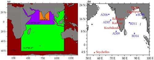
WWIII-version 4.18 model is used for the regional wave forecasting setup at ESSO-INCOIS. The wave model is forced with 3-hourly European Centre for Medium-range Weather Forecast (ECMWF) winds having a spatial resolution of 0.25° × 0.25°. The framework of ECMWF uses the Integrated Forecast System (IFS) using four-dimensional (4D) variational assimilation scheme that assimilates several meteorological observations with ERS-1 and ERS-2 scatterometer winds (Rabier et al. 2000; Janssen 2004). INCOIS-WWIII setup has four mosaic grids in the nested pattern (Global (0°-360°, 80°S-70°N), Indian Ocean (30°E-120°E,60°S-30°N), North Indian Ocean (32°E-100°E, 5°S-29°N) and Coastal (68.5°E-89°E,3.8°N-24°N)), which provides a two-way exchange of information between overlapping grids (Figure 1(a)). The spatial resolution varies from coarser 1° global grid to finer 0.04° coastal grid. The grid preparation has been done with an automated grid generation package V2.2 (Chawla and Tolman 2007). The algorithm in this package is designed to meld the high-resolution bathymetry with the shoreline database to develop the optimum grid. Grids are generated using ETOPO1 bathymetry (1’ arc length global relief bathymetry dataset) from National Geophysical Data Centre and global shoreline database (GSHHS- Global Self-consistent Hierarchical High resolution Shoreline).

Figure 1. (a) Model domain (Global (1° × 1°), Indian Ocean (0.5° × 0.5°), North Indian Ocean (0.25° × 0.25°), coastal (0.04° × 0.04°)) and (b) Buoy locations used for the study.

WWIII integrates the spectral wave energy balance equations in space and time with discretised wave numbers and directions. In the present study, the spectral resolution used is 36 directions and 29 frequencies which are exponentially spaced from 0.035 to 0.5 Hz at an increment of 10%. ST4 source term package is used for wind wave input and dissipation physics (Ardhuin et al.2010). This parameterisation is built around the saturation based dissipation. The conservative terms such as propagation due to local rate of change and spatial and spectral transport terms are balanced by non-conservative sources and sinks. The net source term in the deep water has three components, wind-wave interaction term (S_in), nonlinear wave-wave interaction terms (S_nl) and dissipation (white capping) term (S_ds). In the shallow water, additional processes like wave-bottom interactions (S_bot), depth-induced wave breaking (S_db) and triad wave-wave interactions (S_tr) are also in consideration. The nonlinear wave-wave interactions are modelled using the discrete interaction approximation (DIA) of Hasselmann and Hasselmann (1985). SHOWEX formulation is used for dissipation due to bottom friction (Ardhuin et al. 2003). Third order propagation scheme is implemented with garden sprinkler reduction (Tolman et al. 2002).

2.2. Data used

Firstly, all the available wave buoys in the IO have been used for the validation of wave forecast. Six offshore moored buoys (AD06 (67.45°E, 18.5°N), AD07 (68.9°E, 15°N), AD09 (73.366°E, 8.25°N) located in AS; BD08 (89.67°E, 18.17°N), BD11 (83.96°E, 13.48°N), BD14 (88.08°E,6.99°N) located in BOB basin) are used for validation of the model in the offshore regions. Six wave rider buoys, which are part of WAve Monitoring Along Nearshore (WAMAN) buoy network programme of ESSO-INCOIS (Gopalpur (84.94°E, 19.24°N), Digha (87.79°E, 21.25°N), Karwar (74.05°E, 14.03°N), Kozhikode (75.62°E, 11.3°N), Ratnagiri (73.25°E, 16.95°N) and Seychelles (55.87°E, -4.64°S)) have been taken for validation in the coastal areas. Buoy locations are shown in Figure 1(b). In the offshore buoys, the wave data is measured at a rate of 1 Hz for 17 minutes every three hours and the wind speed and direction are sampled at every second during the 10 minutes measurement period. In the coastal buoys, wave data records were taken at a frequency of 1.28 Hz for 17 minutes every half an hour. Quality checked buoy data are collocated with the model output for the analysis. We have considered wind speed (ws) and seven integral wave parameters for the comparison of model and offshore buoys. Those are significant wave height (Hs), mean period (Tm) and peak period (Tp), swell significant height (Hsa), sea significant height (Hsb), swell mean period (Tma) and sea mean period (Tmb). Directional data was not available for offshore buoys. For the shallow water comparison, we have considered three wave parameters, Hs, Tp and peak directions (Pdir) from the coastal buoys. A threshold frequency criterion of 0.1 Hz is used for swell and sea separation for both buoy and model. All the in-situ observations are located in the NIO and hence, a spatial validation for the IO has been carried out using Jason-2 altimeter wave data, to facilitate the assessment also in the southern IO region. Jason-2 is a low-orbit satellite, equipped with high-precision ocean altimetry that measures the distance between the satellite and the ocean surface, within a few centimetres. Jason-2 datasets are available along the satellite ground track and correspond to an average over swath width 6–7 km along these tracks, with repeat cycles of about 10 days.

2.3. Methodology

The characteristics of a wave can be defined by height, period and direction. Hence, we verified the wave forecast of all parameters related to height, period and direction available from both offshore and coastal observation network. We evaluated the performance in terms of Hs, Hsa, Hsb, Tm, Tma, Tmb, Tp and Pdir. Hs is the average of one-third of the highest waves and is computed as $Hs=4\sqrt{m_0}$. In buoy measurements, for sea and swell separation, the wave spectrum measurements between 0.04 and 0.1 Hz is considered low frequency (swell) components and between 0.1 and 0.5 Hz is taken as high frequency (sea) components. The definition of mean wave period from the buoy is$Tm=\sqrt{{\displaystyle \frac{m_0}{m_2}}}$. Tp (in seconds) is defined as the wave period associated with the most energetic waves in the total wave spectrum at a specific point. The model also follows the same criteria for the sea and swell separation as well as the calculation of wave parameters. The model wave data in the closest sea grid point to each buoy location have been used for validation purposes. The collocation data set is established for the altimeter wind and wave validation using a spatial and temporal window. Selection of the space and time collocation window is very important for the collocation and based on assessments of the spatial and temporal variation of the wave field, Monaldo (1988) proposed the collocation criteria of observations occurring within 50 km and 30 min of one another. The same procedure is adopted here to generate all collocation points for the comparison of satellite altimeter data with model data. The data from the forecast model grids coinciding with the satellite track are extracted first. Satellite data in a particular grid are averaged and collocated with model wave data. These collocated datasets are used for the spatial validation of forecasted Hs. The forecast assessment has been carried for the year 2016 with the observed data (both in-situ and altimeter) in the IO. The performances of the model were evaluated quantitatively by several statistical measures. Statistical error estimation includes bias (Bias), root mean square error (RMSE), correlation coefficient (R) and the scatter index (SI). Error estimation formulae are given below in equations form,$\mathrm{B}\mathrm{i}\mathrm{a}\mathrm{s}=\sum _{i=1}^N\left({\displaystyle \frac{1}{n}\left(y_i-x_i\right)}\right)$ $\mathrm{R}\mathrm{M}\mathrm{S}\mathrm{E}={\displaystyle \frac{1}{n}\sqrt{\sum _{i=1}^N{\left(y_i-x_i\right)}^2}}$ $\mathrm{S}\mathrm{c}\mathrm{a}\mathrm{t}\mathrm{t}\mathrm{e}\mathrm{r}\mathrm{I}\mathrm{n}\mathrm{d}\mathrm{e}\mathrm{x}={\displaystyle \frac{\mathrm{R}\mathrm{M}\mathrm{S}\mathrm{E}}{\overline{x}}}$ $\mathrm{C}\mathrm{o}\mathrm{r}\mathrm{r}\mathrm{e}\mathrm{l}\mathrm{a}\mathrm{t}\mathrm{i}\mathrm{o}\mathrm{n}\left(R\right)={\displaystyle \frac{\sum (x-\overline{x})\ast \left(y-\overline{y}\right)}{\sqrt{{{\sum }^{\left(y-\overline{y}\right)}}^2}\sqrt{{{\sum }^{\left(x-\overline{x}\right)}}^2}}}$

Here y and x represents model and observation wave parameters. $\overline{x}$ denotes the mean of observation.

3. Results and discussions

Here we discuss the results of the INCOIS-WWIII modelled wave field validation with the data from the buoys and the altimeter for the IO. The validation is performed over a one year period for the year 2016.

3.1. Verification of the wave forecast in the offshore areas of NIO

The forecast verification with offshore buoys is described in this section. Observed wave data from six buoys (3 from BOB and 3 from AS; Figure 1(b)) are used for verification of the forecast in NIO. We have selected AD06 and BD08 as the representative locations of AS and BOB basins respectively to show the intra-annual time evolution of wave fields. Figure 2 shows the comparison of forecasted wind speed and wave parameters at AD06. The observed wind shows the clear seasonality, i.e. weak winds (∼10 m/s) during non-monsoon months (pre and post-monsoon) and strong (∼15 m/s) during southwest monsoon winds. The forecast wind follows the pattern of observed winds throughout the year with a positive bias in the monsoon season (Figure 2(a)). The observed wave heights are less than 2 m during the non-monsoon season due to the weak magnitude of prevailing winds. With the onset of monsoon, Hs, Hsa, Hsb have shown an increasing trend and maximum Hs ∼5.5 m is found in the central AS during monsoon (Figure 2(b–d)). The time evolution of the forecast wave heights are in good agreement with the seasonal variability existed in the observation. The comparison of the mean wave period shows some discrepancies during pre-monsoon and post-monsoon periods. The agreement of Tma indicates the accurate forecast of the swell period throughout the year with a slight overestimation during the pre-monsoon period whereas Tmb shows the good agreement only during monsoon (Figure 2(e–g)). It is apparent from the observed Tp that the young swells with Tp ∼10-13 s are the dominant waves in the central AS during monsoon. These young swells were well simulated in the forecast (Figure 2(h)). The wave characteristics changes and the periods are under wilder fluctuation (5–20 s) indicating the coexistence of wind sea and swell during the non-monsoon season (Neetu et al. 2006). Forecasted Tp reproduced the variability of the wave periods (5-20s) in different seasons (SI = 29%; Table 1) and confirms the model capability in forecasting wind sea and swell combined events (Figure 2(h)). From Table 1, where the results of AD06 validation are summarised, it is clear that SI of the all the wave parameters is less than 30%. It is worth mentioning here that the forecast wave parameter with SI of less than 30% is widely accepted by the user community for operational planning (Woodcock and Greenslade 2007). The high SI (29%) and poor correlation (0.47) seen in the Tp are due to the deviations found in the pre-monsoon season.

Figure 2. Comparison of model derived wave parameters with buoy derived wave parameters for Arabian Sea – representative location AD06.

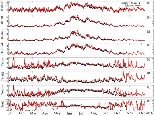
Table 1. Model error statistics for buoy comparison at AD06 location.

Parameters	BIAS	RMSE	R	SI (%)
Ws (m/s)	1.24	1.84	0.90	23
HS (m)	0.14	0.28	0.99	14
Hsa (m)	0.14	0.26	0.97	21
Hsb(m)	0.06	0.21	0.98	14
Tm(s)	0.96	1.36	0.70	17
Tma(s)	0.78	0.96	0.79	5
Tmb(s)	0.58	0.83	0.81	12
Tp(s)	0.74	3.25	0.47	29

Figure 3 shows the comparison of forecast wave parameters at BD08 located in the northern BOB. Observed winds were in the range ∼10 m/s during pre-monsoon season and the magnitude of wind increased during monsoon season (∼15 m/s; Figure 3(a)). The magnitude of winds on some occasions reaches up to∼12 m/during the post-monsoon season depending on the local weather. The forecast wind pattern matches with observation throughout the year irrespective of the season. The statistics of SI = 26% and R = 0.89 (Table 2) confirms a good agreement of the forecast winds with observation. Observed wave heights (Hs, Hsa, Hsb) were less than 2 m during pre-monsoon, whereas the monsoon waves were in the range ∼4–5 m (Figure 3(b–d)). During post-monsoon, wave heights were again decreased to ∼2–3 m. Forecast wave heights follow the trend of observation and shown a very good match at this location. Error statistics values SI (14-23%) and R (0.89-0.97) confirm good agreement of the forecast in the northern BOB region (Table 2). Forecast of Tm and Tmb follows the trend as that of observation during monsoon season, however, deviations are noticed during non-monsoon seasons (Figure 3(a,c)). In the case of the swell period, Tma, the pattern of forecast matches with observation, but a slight overestimation (bias=0.87 s) is seen throughout the year. Deviations are more in the wind sea period especially during pre-monsoon when wave heights are low. Observed Tp shows 10–20 s waves in the northern BOB throughout the year which indicates the dominance of swell in this region. Forecasted Tp reproduced almost all variations in the observation except some high-frequency variation in the non-monsoon seasons (Figure 3(h)). The model was unable to simulate the low wind seas with period ≤ 5s. Table 2 shows the reasonable agreement of the wave periods for operational use with SI (5–27%) and R (0.43–0.7) with the observation in the northern BOB region.

Figure 3. Comparison of model derived wave parameters with buoy derived wave parameters for Bay of Bengal – representative location BD08.

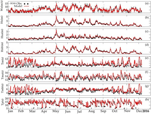
Table 2. Model error statistics for buoy comparison at BD08 location.

Parameters	BIAS	RMSE	R	SI (%)
WS	0.81	1.59	0.89	26
HS	0.13	0.26	0.97	14
Hsa	0.16	0.26	0.89	23
HSB	0.03	0.19	0.97	16
TM	1.43	2.03	0.64	23
TMA	0.87	1.12	0.73	5
TMB	0.84	1.27	0.43	20
TP	1.21	3.5	0.51	28

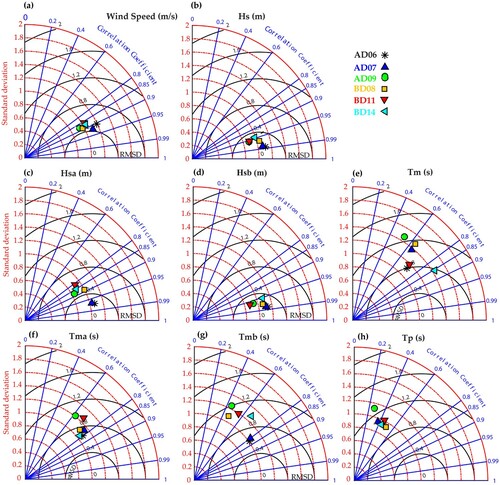
Figure 4(a–h) depicts the Taylor diagrams of observation versus model results for the 6 buoy locations during 2016. From the figure, it can be seen that the model predicted wave heights are in good agreement everywhere. The swell waves are slightly over predicted at all buoy locations, except that of AD06 and AD07. In general, wave heights (Hs, Hsa, Hsb) at all the locations are reasonably correlated within the range of 0.85-0.99 (Figure 4(a–d)). Wave periods are showing more deviations, hence more error and poor correlations which mostly come from the deviation in the wave period existed during the non-monsoon months (Figure 4(e–h)). The mean sea period shows large errors except for AD06 and AD07 whereas the mean swell period shows a good agreement (R> 0.75) in all the locations, except that of AD09 and BD11. Very good agreement of simulated wave parameters is seen in the Arabian Sea buoys AD06 and AD07. From the overall analysis, it can be seen that the model performance for monsoon is satisfactory. But the model is unable to simulate realistically the high-frequency low wind seas during non-monsoon seasons.

Figure 4. Taylor diagram – Symbols represent different moored buoy locations and the different grid axis are the NSTD in dashed lines, the RMSD in black circles, and the correlation coefficient in dashed-dotted lines.

3.2. Verification of the wave forecast in the coastal areas of NIO

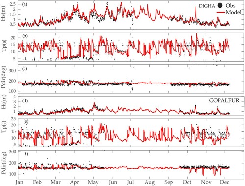
Verification of wave forecast is carried out at 5 coastal locations (Digha and Gopalpur from the east coast of India; Kozhikode, Karwar, and Ratnagiri from the west coast of India) in order to assess the model performance in Indian coastal areas (Figure 1(b)). We also considered off Seychelles buoy (4.64° S, 55.87° E) which is deployed at 15 m depth. Figure 5 shows the comparison of forecasted wave parameters with observation along the east coast, Digha and Gopalpur. Observed wave heights were low most of the time < 1 m in both locations. Tp from the observation shows 10-20swaves throughout the year mostly from south-southeast (150^°-200^°) directions. Such long period swells are mostly from the southern Indian Ocean (SIO) and it indicates that both Digha and Gopalpur are dominated by SIO swells throughout the year. Wave forecast has shown good agreement with observation at these locations.

Figure 5. Comparison of model derived wave parameters with buoy derived wave parameters for east coast of India- representative locations (a–c) Digha and (d–f) Gopalpur.

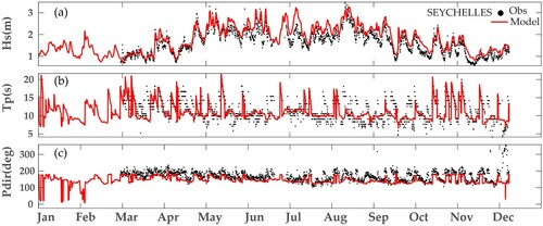
Figure 6 shows the time series comparison of wave parameters at west coast locations, Kozhikode, Karwar and Ratnagiri. At all the three locations, observed wave heights are low (<1.5 m) during the non-monsoon season and high (2–3 m) during monsoon season. Unlike the east coast, a clear demarcation of Tp is seen during monsoon, and the observed Tp is in the range 10–13 s for all the locations (Figure 6(b,e,h)). The coexistence of wind seas and swells (5-20 s) is seen during non-monsoon seasons. Observed directional wave data shows the propagation of waves from the west-southwest directions during monsoon and south-southwest directions during non-monsoon seasons (Figure 6(c,f,i)). The model shows a very good agreement with observation during monsoon, in a similar fashion we have seen in the case of open ocean buoy locations. The interesting fact that is noticed from the observational data is the propagation of shamal swell from the Persian Gulf to the west coast of India during January-March (Figure 6). The increase in wave height and the decrease in period and direction from the North West signify the propagation of shamal swells to the west coast of India during pre-monsoon season (Aboobacker et al. 2011). The swell events are encircled in Figure 6(b, c, e, f, h, i). The forecast from the model is able to reproduce only a few events. It is very clear from the figure that the low wave heights with Tp ∼5s and Pdir ∼300 deg is not well simulated by the model. The deviations are more prominent in pre-monsoon and also seen in the validation in the deep ocean buoy locations. The deviations seen are mostly in the AS which has to be addressed in detail. Perhaps, further tuning of the parameterisation is required for an accurate simulation of these waves and will be addressed in the future study. The model shows good agreement of wave heights with slight overestimation in isolated peaks also at the Seychelles location (Figure 7(a)). The bias seen in the location might be due to the overestimation of the swell. Since the location is more exposed to SIO swell, the observed wave period was mostly seen above 10s as expected (Figure 7(b)). It can also see that the model unable to reproduce a few swell peaks as observed. Model Pdir values are slightly biased anti-clockwise relative to the measurements and mostly waves are from the south-east sector (Figure 7(c)).

Figure 6. Comparison of model derived wave parameters with buoy derived wave parameters for west coast of India- representative locations (a) Kozhikode (b) Karwar.

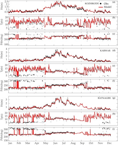
Figure 7. Comparison of model derived wave parameters with buoy derived wave parameters at Seychelles (a) Hs (b) Tp (c) Pdir.

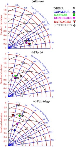
The Taylor diagram gives an overall picture of the performance of the model in the coastal regions (Figure 8). The diagram describes the verification of the wave forecast at each buoy location in terms of RMSE, Standard deviation and Correlation. All statistics together represent the accuracy level of the forecast. Wave heights are in very good agreement in all the locations(R>0.9) (Figure 8(a)). The large errors seen in the period and direction are mainly due to the deviations in the non-monsoon seasons (Figure 8(b,c)). Overall analysis shows that the accuracy of the forecast in the coastal region is also good enough for operational use.

Figure 8. Taylor diagram – Symbols represent different coastal buoy locations and the different grid axes are the NSTD in dashed lines, the CRMSD in black circles, and the correlation coefficient in dashed-dotted lines.

3.3. Validation with altimeter data

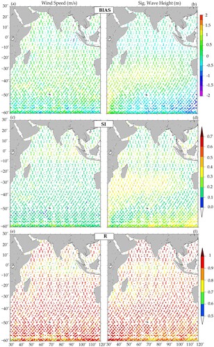
Here we present the spatial validation results obtained comparing the satellite altimeter data (along-track comparison) and the corresponding WWIII data for the considered one year period (Figure 9). Spatial maps of the error statistics are shown in Figure 9. Compared with Jason-2 Hs data, the model mean bias is in the range −0.5–0.5 for the NIO mostly in correlation with wind biases (Figure 9(a,b)). The mean bias for the southern ocean belt50°S-20°S is high (∼1 m) compared to other regions. SI is found to be less than 30% in the NIO regions and the error is more in the above said Southern Ocean belt (40-50%). Very good correlation (R>0.8) of Hs is obtained in the whole IO domain (Figure 9(f)). The errors in the wave heights have mostly resulted from forecast wind errors (Figure 9(a)). The spatial validation of the model with satellite data also proves the reliability of the model results in the IO, which endorses the usage of the developed wave forecasting system for operational use.

Figure 9. Spatial error statistics for the model comparison with altimeter (a–b) BIAS (c–d) SI (e–f) R; Left panel: wind speed (m/s), Right panel: Significant wave height (m).

3.4. Verification of wave forecast during extreme events

As already discussed, the high wave conditions in the Indian Ocean are mainly due to monsoon winds, tropical cyclones and southern ocean wind conditions. In the above sections, the validation during monsoon has been described. In this section, we provide the validation during other two extreme wave conditions (i) Tropical cyclone (ii) The Kallakkadal event due to SIO swell.

3.4.1. Validation of wave forecast during tropical cyclones

During our study period, NIO, or more specifically, BOB witnessed one of the very severe cyclonic storms Vardah and three other cyclonic storms namely Roanu, Kyant, and Nada. Figure 10 shows cyclone track (taken from Indian Meteorological Department (IMD)) along with respective periods of occurrences and the buoy locations which are taken into consideration for the analysis. Table 3 summarises the details of cyclones over BOB. Reliability of the forecast during Roanu cyclone is explained in detail below and an overall statistics are shown for other cyclones. Cyclone Roanu was formed on 14th May near south of Sri Lanka having wind speed of 23 m/s headed northward and dissipated over Gangetic West Bengal on 21st May. From Figure 10, it can be seen that BD08 and BD11 buoy are located near the track of this tropical cyclone and can be used for comparison of wave parameters. Cyclone travelled from south to north direction, so initially, BD11 experienced a maximum wave height of 5.6 m, and the model simulation generated a wave height of 5 m on 19^th May 12 UTC (Figure 11(a)). Peak period observed at BD11, which is the period of maximum wave energy generated due to the cyclonic storm is 9.3s and simulation is showing 9.2s on 19^th May 12 UTC. At BD08, the observed Hs has increased gradually and reached a peak value of 5.7 m, and the simulated model output has shown a minor underestimation of 0.4 m on 21st May (Figure 11(b)).

Figure 10. Track of cyclonic storms as per IMD best track preliminary report. Tracks of Roanu, Kyant, Vardah and Nada ( lines) and buoy locations (circles and squares) near to the tracks are represented.

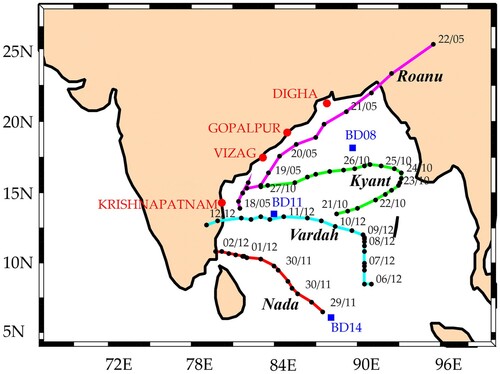
Figure 12. Comparison of wave forecast with observations during cyclone Roanu (a–b) Deep Ocean (c–e) Coastal Ocean.

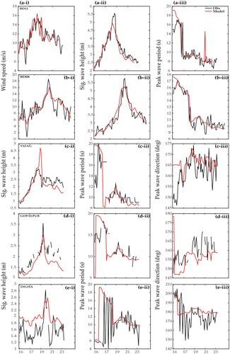
Table 3. BOB tropical cyclones information during 2016.

Cyclone name (TC)	Period 2016	Buoys near TC track
Roanu cyclonic storm	17th May–22nd May	BD11, BD08, Gopalpur and Digha
Kyant cyclonic storm	21st Oct–28th Oct	BD08, BD11 and Krishnapatnam
Nada cyclonic storm	29th Nov–2nd Dec	BD11 and Pondicherry
Vardah very severe cyclonic strom	6th Dec–13th Dec	BD11, BD14, Port Blair and Krishnapatnam

The movement of Cyclonic storm Roanu was parallel to the east coast of India and hence all the coastal buoys (Krishnapatnam, Vizag, Gopalpur and Digha) were happened to lie on the left side of the cyclone track (Figure 10). At Vizag location, model simulated Hs has shown an overestimation of ∼1 m at the peak, which might be attributed to the wind error (Figure 11(c)). Tp and Pdir show good agreement with observed values during the cyclone period. Gopalpur location shows maximum Hs∼3.5 m for buoy and model forecast was Hs ∼3 m at 20th May 09 UTC (Figure 11(d)). The agreement of Tp also was good during this period. Predicted Pdir showed some deviations from the observed direction, and the average difference was ∼10 deg. It can be seen from the figure that, at Digha location, model picks the peak Hs (2.6 m) on 21st May 00 UTC with a 6-hour lag when compared with observation (Hs=2.8 m which is on 20^th May 18 UTC) (Figure 11(e)). Pdir and Tp were in good agreement in this case also.

Table 4 provides the model error statistics for different cyclones. The statistics support the reliable performance of the model during cyclone Roanu with low SI (for Hs, 16%; for Tp, 30%) and good correlation (for Hs, 0.91; for Tp,0.54). During the cyclone Kyant, comparison shows a high correlation of 0.91, the low negative bias of −0.09 m, low RMS error of 0.21 m and SI of 15% for Hs (Table 4). SI for Tp (25%) also is within the acceptable range for operational use. During Nada cyclone, the model shows low bias (for H,−0.04 m; for Tp, −0.06 s), low SI (for Hs, 14%; for Tp, 31%) and high correlation (for Hs, 0.95; for Tp, 0.97). The combined statistics reveal that, during the cyclone Vardah, wave height forecasts were highly accurate, which is evident from a high correlation of 0.95, the low negative bias of −0.15 m, low RMS error of 0.37 m and SI of only 15%.

Table 4. Model error statistics for the buoy comparison during different tropical cyclone periods.

Cyclone/parameter	BIAS	RMSE	R	SI (%)
ROANU (BD11, BD08, Gopalpur and Digha)
Hs (m)	0.04	0.39	0.91	16
Tp (s)	0.62	3.44	0.54	30
KYANT (BD08, BD11 and Krishnapatnam)
Hs (m)	−0.09	0.21	0.91	15
Tp(s)	0.13	2.56	0.54	25
NADA (BD11 and Pondicherry)
Hs (m)	−0.04	0.18	0.95	14
Tp (s)	−0.06	0.82	0.97	31
VARDAH (BD11, BD14, Port Blair and Krishnapatnam)
Hs (m)	−0.15	0.37	0.95	15
Tp (s)	0.93	3.07	0.41	34

3.4.2. Validation of wave forecast during swell event

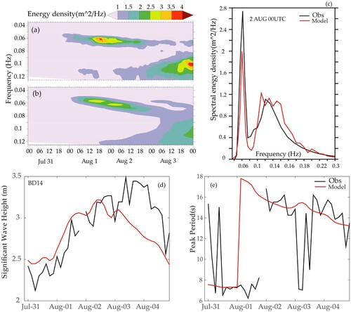
High swell events and coastal flooding are quite frequent in the Indian coastal areas. The link between such events and the Southern Ocean meteorological conditions are already explored in the study of Remya et al. (2016). Hence forecast evaluation during the swell event is very important and one such case is analysed here. High swells from the Southern Ocean affected the regions of Kerala, south Tamil Nadu and West Bengal from 31^st July to 4^th August 2016 (furnished based on user feedback). A storm developed in the Southern Ocean (near50°S and 90°E) on 26^th July 2016 was responsible for the high swell generation. The wind speed and Hs at the generation area was 24 m/s and 12 m respectively (not shown). The swell waves with period 18.13s hit the Kozhikode location on 1st August 15 UTC. As per model results, the first swell wave with period 18.8s hit the location on 1^st August 3 UTC. Model simulation shows a lead of 12 hours in the arrival time of swells at the buoy location. An overestimation in wave periods is also seen along with a lead of 12 hours. In the deep ocean, the group velocity can be directly linked to the wave period and hence any overestimation in the wave period can lead to an increase of wave velocity. An increase in the velocity will cause a lead in the time of hit of swell trains in different places. Spatial validation of wind shows a positive bias in the SIO and hence the error in the swell waves might be due to the error in the swell source wind (Figure 9(a)). The time evolution of spectra for both observation and model at Kozhikode location is shown in Figure 12(a,b). Spectral shapes show a good agreement with an underestimation in maximum energy (>0.5m²/Hz) during the period. Figure 12(c) shows a comparison of spectra at 00UTC of 2^nd August. A very good match of spectral shape can be seen in both low and high frequencies. The dominant low frequency peak was seen around 0.06 Hz in both model and observation, but the model could not accurately reproduce the maximum energy at the low frequency and it shows an energy underestimation of ∼0.8m²/Hz in dominant frequency. Also at the deep ocean location BD14, the model simulation shows a lead of 21 hours in the travel time and overestimation in the periods. In the model results, the first swell wave with period 17.79s hit the location BD14 on 1^st August 03 UTC whereas the observations 16.8s on 2^nd August 00 UTC (Figure 12(d,e)). Model Hs shows good agreement with observation till 3^rdAugust. The underestimation seen in Hs during 3–4 August was attributed to the wind error (not shown). Tp also shows a very good match with observation with a lead of 18 hours in the swell arrival time. A detailed comparison of southern ocean wave conditions may reveal the reason for the lead which cannot be performed in this study due to the lack of observed data. Overall analyses suggest that the model is able to predict the swell events with a good level of accuracy and can be used for operational high period swell predictions.

Figure 12. Timeevolution of wave spectrum shows the strong swell event during 31, July 31–4, August, 2016 at Kozhikode.(c) Comparison of wave spectra on 2 August,2016-00 UTC, Bottom panel (d-e) Hs and Tp comparison during swell event at off shore location BD14.

4. Conclusions

This study provides an extensive validation of the performance of the WAVEWATCH-III regional wave forecasting setup at ESSO-INCOIS, India. Such a wave forecasting system was developed by fine tuning the WW-III model for the Indian Ocean basin using a large amount of data from observational platforms deployed in the IO region. The study period for evaluation of the model forecast is one-year i.e. January–December 2016. The wind fields used for the model forcing are from ECMWF. The verification of the forecast is done using all the available in-situ and satellite data for the IO. The verification is done separately for deep ocean and coastal ocean areas. The model error statistics suggest that the model simulated wave parameters are very accurate in the monsoon for both coastal and open oceans. Non-monsoon months are showing discrepancies in the simulated wind seas especially when the wave heights are very low. The correction of such discrepancies may require further research and tuning of parameterisation schemes in the model and will be addressed in future work. Model performance during cyclones Roanu, Kyant, Nada, and Vardah again supports the reliability of the WW-III wave forecast for both open and coastal areas. Model performance is evaluated during the coastal flooding events known as Kallakkadal showed a lead in the arrival of swell in different locations compared to observations which are mostly resulted from an overestimation of wave period in the model. However, the wave spectra comparison at specific times shows good agreement of spectral shapes. In a nutshell, the overall analysis and the model error statistics for various intra-annual conditions in the Indian Ocean ensured the reliability of the WW-III generated wave forecasts, and this particular WW-III wave model setup can be used for operational use with high confidence and better reliability. The discrepancies found in the model can be improved through further research, for instance, tuning of parameterisation schemes in the wave models, data assimilation, etc., which will eventually lead to further betterment of the existing forecast set up. That will be our future focus of research.

Acknowledgements

We thank R. Venkat Sheshu, Ramakrishna Phani,N Arun, Jaykumar and Ramesh (ESSO–INCOIS) for providing the in-situ data. We specially thank Mr. Kaviazhahu for his technical support for the setup of the regional wave forecast system in HPC. The moored buoy data for the analysis was provided by ESSO–NIOT. We thank two anonymous reviewers for their constructive comments and suggestion on the manuscript and its eventual improvement. Special thanks to the editor for his valuable comments and editorial corrections. We thank our Director, INCOIS for the encouragement and support. We also thank Earth System Science Organization, Ministry of Earth Sciences, Government of India for financial support. This is ESSO–INCOIS contribution 371.

Disclosure statement

No potential conflict of interest was reported by the author(s).

Additional information

Funding

This work was supported by Earth System Science Organization, Ministry of Earth Sciences, Government of India.

References

- Aboobacker VM, Rashmi R, Vethamony P. 2011. Shamal swells in the Arabian Sea and their influence along the West Coast of India. J Geophys Res Lett. 38:L03608.
- Ardhuin F, Herbers THC, Jessen PF, O’Reilly WC. 2003. Swell transformation across the continental shelf, part II: validation of a spectral energy balance equation. J Phys Oceanogr. 33:1940–1953.
- Ardhuin F, Rogers E, Babanin A V, Filipot J F, Magne R, Roland A, vanderWesthuysen A, Queffeulou P, Lefevre JM, Aouf L, Collard F. 2010. Semi- empirical dissipation source functions for ocean waves. Part I: definition, calibration, and validation. J Phys Oceanogr. 40:1917–1941.
- Bhowmick S, Kumar R, Chaudhuri S, Sarkar A. 2011. Swell propagation over Indian Ocean region. Int J Ocean Clim Syst. 2(2):87–99.
- Chawla A, Tolman HL. 2007. Automated grid generation for WAVEWATCH III. Tech. Note 254, NOAA/NWS/NCEP/MMAB, 71 pp.
- Hasselmann S, Hasselmann K. 1985. Computations and parameterizations of the nonlinear energy transfer in a gravity wave spectrum, I, a new method for efficient computations of the exact non-linear transfer integral. J Phys Oceanogr. 15:1369–1377.
- Janssen P. 2004. The interaction of ocean waves and wind. Cambridge, U.K: Cambridge University Press. 300 pp.
- Janssen P. 2008. Progress in ocean wave forecasting. J Comput Phys. 227(7):3572–3594.
- Komen GJ, Caveri L, Doneland M, Hasselmann K, Hasselmann S, Janssen PAEM. 1994. Dynamics and modelling of ocean waves. Cambridge, U.K: Cambridge University Press. UK-560.
- Kurian NP, Nirupama N, Baba M, Thomas KV. 2009. Coastal flooding due to synoptic scale, meso-scale and remote forcings. Nat Hazards. 48:259–273.
- Mohanty UC, Osuri KK, Routray A, Mohapatra M, Pattanayak S. 2010. Simulation of Bay of Bengal tropical cyclones with WRF model: impact of initial and boundary conditions. Mar Geodesy. 33:294–314.
- Monaldo F. 1988. Expected differences between buoy and radar altimeter estimates of wind speed and significant wave height and their implications on buoy-altimeter comparisons. J Geophy Res. 93:2285–2302.
- Neetu S, Shetye S, Chandramohan P. 2006. Impact of sea breeze on wind-seas off Goa, west coast of India. J Earth Syst Sci. 115:229–234.
- Rabier F, Jarvinen H, Klinker E, Mahfouf JF, Simmons A. 2000. The ECMWF operational implementation off our-dimensional variational assimilation. I: Experimental results with simplified physics. QJR Meteorol Soc. 126:1143–1170.
- Remya PG, Kumar R, Basu S, Sarkar A. 2012. Wave hindcast experiments in the Indian Ocean using MIKE 21 SW model. J Earth Syst Sci. 121:385–339.
- Remya PG, Vishnu S, Praveen Kumar B, Balakrishnan Nair TM, Rohith B. 2016. Teleconnection between the North Indian Ocean high swell events and meteorological conditions over the southern Indian Ocean. J Geophys Res Oceans. 121(10):7476–7494.
- Tolman HL. 1991. A third-generation model for wind waves on slowly varying, unsteady and inhomogeneous depths and currents. J Phys Oceanogr. 21:782–797.
- Tolman HL, Balasubramaniyan B, Burroughs LD, Chalikov DV, Chao YY, Chen HS, Gerald VM. 2002. Development and implementation of Wind-Generated Ocean Surface Wave Models at NCEP. NCEP notes. Camp Springs, MD: NOAA/NCEP/Environmental Modelling Centre.
- Woodcock F, Greenslade DJM. 2007. Consensus of numerical model forecasts of significant wave heights. Weather Forecast. 22:792–803.