Evaluating pressure gauges as a potential future replacement for electromagnetic cable observations of the Florida Current transport at 27°N

ABSTRACT

For 30+ years, submarine cable voltage measurements have been a critical measurement system used to produce a highly valuable time series of daily Florida Current volume transport at 27°N in the Florida Straits. However, the high cost associated with replacing the measurement system, should the existing telecommunications cable break, represents a significant vulnerability to the continuation of this important transport time series. Six years of data from tide gauges near the ends of the cable at 27°N have been used to test the potential of a paired tide gauge system to replace the cable in the event of a future problem. Validations against the daily cable observations, and against snapshot transport estimates from ship sections, suggest that the tide gauges do represent a viable replacement, however, the accuracy of the transports determined from the tide gauges is lower than for the cable observations (2.7 Sv vs. 1.7 Sv, respectively). The tide gauges capture roughly 55% of the total variance observed by the cable. The correlation between the cable data and the tide gauge differences is fairly constant (r ≈ 0.75) after low-pass filtering the data at periods from 3 to 365 days, illustrating a lack of coherence sensitivity to those time scales.

KEYWORDS:

• Florida Current
• Gulf Stream
• flow measurement
• volume transport
• sea level

Introduction

The insightful idea of measuring voltages induced on a subsurface telecommunications cable in order to estimate the volume transport of the Florida Current across the cable was first presented by Stommel (1948), although implementation of the idea on a cable between Key West and Havana initially proved quite challenging (e.g. Wertheim 1954; Stommel 1957, 1959, 1961). Later work by Sanford (1982) and Larsen and Sanford (1985) demonstrated that the concept represented a fully viable method for monitoring the Florida Current volume transport farther north near 27°N. The work of these researchers, and those that followed, has resulted in the longest quasi-continuous time series of daily volume transports for any major oceanic boundary current on earth, extending for more than 35 years to date (e.g. Meinen et al. 2010, and the references therein). The modern cable observations have been carefully validated against many repeated ship section transport observations, and the daily measurements of volume transport from the cable, between 2000 and the present, have been shown to be accurate to within 1.7 Sv (1 Sv = 10⁶ m³ s⁻¹), with annual average cable transport estimates accurate to within 0.3 Sv (Garcia and Meinen 2014). The Florida Current transport time series is a key component of the trans-basin meridional overturning circulation array at 26.5°N (e.g. McCarthy et al. 2015; Smeed et al. 2018), and the robust mean value and long time series is often used to validate/test a wide range of numerical ocean models (e.g. Mooers et al. 2005).

Given the strong scientific value of the long Florida Current transport time series, efforts have been underway for several years to determine a potential replacement observing system for the inevitable but unknown future date when the existing submarine cable breaks. The cable used for observing the Florida Current has broken before, however when that occurred a similar alternate telecommunications cable was available for immediate reinstrumentation with voltage measuring equipment (e.g. Larsen 1991, 1992). No such backup exists today. The presently instrumented cable has been out-of-service for telecommunications purposes since 1998, and although efforts have been made, permissions to instrument the active fibre-optic telecommunications cable through the region have not yet been obtained. As laying a cable solely to continue the time series is well beyond the budget levels available for scientific research, alternate technologies and methods have been the focus of future resilience and planning for this key ocean observation.

Prior theoretical work (e.g. Wunsch et al. 1969; Schott and Zantopp 1985) and observational research comparing the cable measurements to tide gauge data on either side of the Straits of Florida (e.g. Maul et al. 1985, 1990) have suggested that paired tide gauges might be a possible technology applicable for accurately observing the volume transport of the Florida Current. While the idea of using sea level observations on either side of the Florida Current has been around for a very long time (e.g. Montgomery 1938; Wunsch et al. 1969), putting the idea into practice has been more challenging due to the limited observations available, particularly on the eastern side of the Straits of Florida.

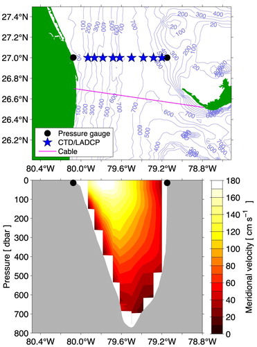
A new six-year record of tide gauge/pressure gauge observations near the 12 m isobath on either side of the Straits at 27°N from July 8, 2008 to September 17, 2014 provides the opportunity to test this potential method for observing the Florida Current volume transport much more directly, with gauges that are well-situated in relation to the cable (Figure 1). Furthermore, during this recent time period a significant number of high-quality shipboard surveys across the section were conducted: 33 which include dropsonde observations at nine sites spanning the Straits (Figure 1); and 24 which include lowered acoustic Doppler current profiler (LADCP) data current velocity profiles collected at each of these same nine stations (e.g. Garcia and Meinen 2014; Meinen et al. 2016). This collection of intensive ship-based observations allows for careful testing and validation of the pressure gauge differences as an alternate method for observing the Florida Current transport at 27°N.

Figure 1. Top – Map of the study region with the nominal locations of the observations indicated – dropsonde observations are collected at the same sites as the CTD/LADCP. Contours represent bottom depth from the Smith and Sandwell (1997) data set; solid green indicates land. Note: the global Smith-Sandwell topography data set does not reproduce well the fine details around the Bahama Banks – the eastern pressure gauge is actually at about 13 m depth despite the contours shown in the plot. Bottom – Vertical section of meridional velocity from repeated LADCP observations at the nine stations shown in the top panel. All LADCP sections collected during July 2009 through September 2014 were averaged for this section. Pressure gauge locations are indicated by the black dots. Bottom topography (directly measured) indicated in gray in the lower panel is based on averages from repeat ship sections along the section in the 1980s and 1990s courtesy of Jimmy Larsen.

Data

The analysis presented herein is based on two different types of continuous time series observing systems, the cable voltage observations and the measurements made by pressure/tide gauges, and two different types of snapshot ship systems, LADCP and free-falling dropsonde floats.

The voltage measurements recorded on the cable, and the methods involved in converting these voltages into daily estimates of Florida Current volume transport, have been well documented over the past few decades (e.g. Larsen and Sanford 1985; Meinen et al. 2010). The observations of the free-falling dropsonde floats and the LADCP observations made in the Straits of Florida, as well as the processing of these two data sets into volume transport measurements, have also been presented previously in Garcia and Meinen (2014) and Meinen et al. (2010). The intercomparison of these three systems, presented in Garcia and Meinen (2014), found that the daily cable, dropsonde, and LADCP volume transport estimates are accurate to within 1.7, 0.8, and 1.3 Sv, respectively. A total of 24 LADCP sections and 33 dropsonde sections were collected during the pressure gauge period presented herein. The locations where the ship section observations are collected, and the nominal endpoint locations for the cable, are presented in Table 1 and Figure 1.

Table 1. Nominal locations of the moored and shipboard observations. The endpoints for the cable are near West Palm Beach (26° 42’N, 80° 04’W) and Eight Mile Rock (26° 31’N, 78° 47’W).

Site Name	Observation Type(s)	Nominal Latitude	Nominal Longitude	Depth (m)
Pwest	pressure gauge	27° 00.1’N	80° 04.6’ W	12
Peast	pressure gauge	27° 00.1’N	79° 08.9’ W	13
Station 0	CTD/LADCP & dropsonde	27° 00.0’N	79° 55.8’ W	139
Station 1	CTD/LADCP & dropsonde	27° 00.0’N	79° 52.0’ W	261
Station 2	CTD/LADCP & dropsonde	27° 00.0’N	79° 47.0’ W	389
Station 3	CTD/LADCP & dropsonde	27° 00.0’N	79° 41.0’ W	540
Station 4	CTD/LADCP & dropsonde	27° 00.0’N	79° 37.0’ W	661
Station 5	CTD/LADCP & dropsonde	27° 00.0’N	79° 30.0’ W	783
Station 6	CTD/LADCP & dropsonde	27° 00.0’N	79° 23.0’ W	708
Station 7	CTD/LADCP & dropsonde	27° 00.0’N	79° 17.0’ W	624
Station 8	CTD/LADCP & dropsonde	27° 00.0’N	79° 12.0’ W	485

The pressure/tide gauges used in this study were Sea-bird Electronics 26plus Seagauge Wave & Tide Recorders (SBE26plus) set to collect pressure data every 5 min (averaging a burst of 60 samples over a 1-min interrogation window). The manufacturer states a resolution for these sensors of 0.2 mm. The absolute accuracy of the sensors is nominally irrelevant here, as only the temporal variations from the record-length mean are used in the presented calculations. The manufacturer also estimates the stability of the sensors (i.e. the long-term drift) to be 0.02% of full-scale per year, or 6 mm per year; in practice, the drifts in the sensors presented here have been much smaller. Sea level rise associated with climate change (global average ∼ 1–3 mm/year; e.g. Church and White 2011) can theoretically be observed with these sensors, however the signals associated with Florida Current variability are one to two orders of magnitude larger than the sea level rise signals, and thus dominate the observed records. Each gauge was deployed for a period of nominally one year in a rigid mount set on the ocean bottom at a nominal depth of 12 m. At the end of each deployment, the SBE26plus recorders were recovered by scuba divers, cleaned of biofouling, fitted with fresh batteries, and redeployed. Due to ship and/or diver availability issues, some of the deployments were longer than the planned one year, however all sensors recorded data for the full duration of each deployment. As will be discussed shortly, during one deployment at the western pressure gauge site, an instrument experienced a problem that resulted in the loss of several months of data. The locations of the moored pressure gauges are shown in Table 1 and Figure 1.

Methods

The first step in merging the ∼1-year-long pressure records into a continuous time series was removing the record-length mean from each deployment. Once the record length mean from each pressure gauge was removed, the back-to-back records at each site were combined together to provide a continuous ∼six-year time-series of 5-min pressure anomalies at each of the two sites (Figure 2). In principle, the removal of the record-length mean from each ∼1-year-long deployment might also reduce and/or eliminate all interannual signals in the pressure records. In practice, however, the precise length of each deployment was never exactly one year, so the variance removed was not at a uniform time scale. Nevertheless, it is important to note that interannual variance might be suppressed by the use of 1-year-long-records from the pressure records. Previous analysis of the cable data has suggested that interannual variability represents only a small percentage (<10%) of the total variance in the Florida Current variability (Meinen et al. 2010). In the future, interannual variations could be better captured by using longer pressure gauge records and/or by overlapping pressure records at each site.

Figure 2. Top: Raw 5-min pressure anomalies from western location. Middle: Raw 5-min pressure anomalies from eastern location. Bottom: Daily average pressure anomalies after a simple 3-day low-pass filtering; note smaller y-axis scale in bottom panel. Vertical black dashed line indicates problematic turn-around discussed in text.

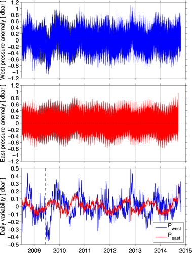
Once the two ∼6-year-long records (west and east) were generated from the individual deployments, the peak-to-peak range of the western gauge was found to be from −1.078 dbar to +1.112 dbar, while the peak-to-peak range of the eastern gauge spanned −0.763 dbar to +0.980 dbar. A simple three-day low-pass filter (2nd order Butterworth, passed both forward and back to avoid phase shifts) illustrates a problem that occurred at the turn-around at the end of the first deployment of the west gauge (Figure 2, bottom panel). The black vertical dashed line in the bottom panel of Figure 2 indicates the date of the pressure gauge turn-around, which coincides with a strong downward jump in the pressure. This is clearly artificial, and appears to have resulted from the cleaning of biofouling from the sensor. After a few months, by the start of October 2009, the values approach a more reasonable range. For the purposes of this study, the data from the turn-around date on 15 June 2009 through 1 October 2009, have been removed from the west pressure gauge record. The choice of the endpoint of the problem period is subjective, however modest adjustments of this cut-off have no significant effect on the results presented.

The standard deviation of the unfiltered 5-min pressure records (after excising the aforementioned problematic period from the west record) is 0.343 dbar for the west gauge, and 0.316 dbar for the east gauge. The dominant signals in these pressure records are of course the tides. The harmonic analysis technique allows for the estimations of the amplitudes and phases of various tidal constituents contributing to the west and east pressure variability (e.g. Emery and Thomson 1997); here the t_tide harmonic analysis software package produced by Pawlowicz et al. (2002) was employed to estimate the amplitudes and phases of 68 tidal constituents. The amplitudes and phases of the six largest-amplitude constituents are shown in Table 2. The largest constituents are the same for both pressure gauges, and for the most part the amplitudes and phases are quite similar. The purpose of this paper is not to delve deeply into the tides within the Florida Straits – which has been studied repeatedly in the past (e.g. Niiler 1968; Wunsch and Wimbush 1977). However, while the tide gauge sites for this experiment were selected for their suitability, some tidal analysis and validation is warranted to confirm that these new instruments were not placed in constricted channels or otherwise unrepresentative locations.

Table 2. Statistics for the six largest-amplitude tidal constituents found through harmonic analysis of the pressure records. Note that the same six constituents were the largest in both pressure records, however the order of amplitude was not the same in the two records. Units: tidal frequencies are in cycles per day; amplitudes are in decibars; phases are in degrees relative to Greenwich. Errors shown for both amplitude and phase are 95% confidence limits. The complete record was used for the east side; for the west side the record beginning on 1 October 2009 was used to avoid the problematic time period discussed in the text where one of the gauges was clogged with debris.

Tide constituent		West side		East side
Name	Frequency (cycles/day)	Amplitude (dbar)	Phase (° rel. Greenwich)	Amplitude (dbar)	Phase (° rel. Greenwich)
S2	2.000	0.074 ± 0.001	40.3 ± 0.5	0.073 ± 0.001	41.1 ± 0.6
M2	1.932	0.418 ± 0.001	12.1 ± 0.1	0.408 ± 0.001	11.2 ± 0.1
N2	1.896	0.100 ± 0.001	352.2 ± 0.4	0.098 ± 0.001	350.3 ± 0.4
K1	1.003	0.072 ± 0.001	216.4 ± 0.6	0.066 ± 0.001	197.5 ± 0.5
O1	0.930	0.057 ± 0.001	223.9 ± 0.7	0.047 ± 0.001	203.4 ± 0.9
SA	0.003	0.086 ± 0.018	316.3 ± 12.8	0.063 ± 0.006	218.5 ± 5.7

The tide amplitudes and phases recorded by these gauges were found to be similar to those measured by the current meter records and tide gauges from the STACS experiment in the 1980s (e.g. Mayer et al. 1984), particularly their Jupiter Inlet gauge, at least in terms of the diurnal and semi-diurnal tidal amplitudes and phases. The statistical accuracy of the amplitudes and phases found herein are roughly an order of magnitude better than were available in the earlier studies (e.g. Wunsch and Wimbush 1977) – most likely due to the much longer time series available here (multiple years versus 2–5 months). Given this good agreement, it is safe to conclude that the sites selected for this study are reasonable, and that the sites are not affected by constricted bathymetry or associated small-scale hydrodynamics. These pressure gauges should therefore be representative of the large-scale geostrophic flows within the Straits. The locations of the tide gauges used herein is about as ideal as is possible given their position relative to the cable (Figure 1); these locations are far more advantageous than some of the locations used in earlier studies (e.g. at Key West to the south or Patrick Air Force Base to the north, where some of the gauges used by Mayer et al. 1984 were located).

Because the cable observations cannot be used to study time scales shorter than three days due to the 72-h low-pass filtering inherent in the data processing (e.g. Meinen et al. 2010), for the comparison purposes the tides must be removed from the pressure gauge records and a similar low-pass filter must be applied. Therefore, the pressure data were filtered with a 2nd order Butterworth filter, passed both forward and back to avoid phase shifts, with a 72-h cutoff period. The filtered data were then averaged within 24-h windows centred on noon GMT to produce a daily time series of pressure at each site. When normalized data are discussed, the records were normalized by removing the record-length mean and dividing by the standard deviation.

Results and discussion

The pressure gradient variability, calculated as P_east minus P_west, should be directly comparable to the cable transport variability if the pressure gauges are to be a viable option for monitoring the Florida Current transport (Figure 3(a)). Maul et al. (1985) also argued that the negative of the west side pressure (-P_west) would also be a good representative of the Florida Current transport, so that is also presented in Figure 3(a). Even after the 72-h low-pass filtering, there is still a great deal of high-frequency energy in the records that makes comparison of the time series visually challenging, so plots of the normalized cable transport versus the normalized pressure difference (P_east – P_west) and versus the normalized west side pressure (-P_west) are also presented (Figure 3(b,c)). While it is clear from these comparisons that there is some correspondence between the cable measurement variability and the pressure difference variability and/or the negative west pressure variability, the relationship is clearly not a clean one-to-one relationship in either case.

Figure 3. (a) Daily time series of the Florida Current volume transport from the submarine cable (green), the eastern pressure anomaly record minus the western pressure anomaly record (magenta), and the western pressure anomaly record multiplied by −1 (blue). (b) Scatter plot of the daily cable values and the corresponding daily pressure differences. (c) Scatter plot of the daily cable values and the corresponding daily western pressure anomalies multiplied by −1. Angle brackets indicate that all values have been normalized by removing the record-length mean and dividing by the standard deviation of the daily values.

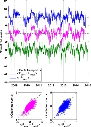
The correlation coefficient between the cable transports (normalized) and the east minus west pressure difference (normalized) is r = 0.76, and the correlation coefficient between the normalized cable record and the normalized negative west pressure record is r = 0.73. Although the difference in the correlation values is quite small, clearly one cannot state that there is a better correlation with the negative west pressure than with the pressure difference. Both of these correlation values are relatively modest, and a linear relationship between either the pressure difference or the negative west pressure and the cable transports would explain only about r² ≈ 55% of the variance in the cable time series (e.g. Emery and Thomson 1997).

Maul et al. (1985) used monthly-mean values of sea level observations from tide gauges at Miami, Florida, and Cat Cay, Bahamas, for comparison with the Florida Current cable observations. The time period for their comparison was April 1982 through September 1983, so a period of roughly a year and a half. They reported very high r² values for their comparisons of both the pressure difference across the Straits and the negative west side pressure. Their r² values were greater than 0.9, which indicates that their correlation values were roughly r = 0.95. It is important to note that the tide gauges utilized by Maul et al. (1985) were from coastal stations that are not nearly as well situated for constraining flow as the new pressure gauges presented here. In particular, the Bahamian tide gauge at Cat Cay, which Maul et al. (1985) used, was situated south of the Northwest Providence Channel. There is a small but significant and variable flow through the Northwest Providence Channel that enters the Florida Current south of the cable location and north of Cat Cay (e.g. Richardson and Finlen 1967; Leaman et al. 1995; Johns et al. 1999). With this in mind, it is hard to reconcile the Maul et al. (1985) high correlations with the lower correlation values presented here.

One potential explanation would be that this difference from the earlier results is an issue of time scale, i.e. comparing results from daily observations (presented herein) versus the monthly observations used by Maul et al. (1985). However, correlating monthly averages of the modern data (pressure differences versus cable transports, or P_west versus cable transports) gives essentially the same result as the daily values (r = 0.77 versus r = 0.76, or r = 0.73 versus r = 0.73, respectively). Evaluating the time scales within the different records does yield some interesting clues though. Comparing the seasonal cycles of the modern records (Figure 4) demonstrates that while the P_east seasonal climatology is quite different from the cable, the P_west climatology compares fairly well with that of the cable (after flipping the sign as appropriate), and the difference (P_east – P_west) climatology is extremely similar to that of the cable. This suggests that the majority of the disparity between cable and pressure gauge difference is at time scales other than seasonal. Interestingly, correlating the cable and pressure differences within individual months (e.g. daily values in January) or by season (e.g. daily values in December-February) suggests that the correlation between cable transports and pressure gauge differences is high in autumn and winter (r ∼ 0.84) and low in spring and summer (r ∼ 0.60). With only six years of data these results are clearly preliminary, and will require further study with longer records, but the result suggests some seasonality to the pressure gauge/cable comparison. Returning to the year-round cable/pressure gauge comparison disparity, a more detailed spectral analysis of the time series presented here demonstrates clearly that the disparity between cable transports and pressure gauge differences is complicated (Figure 5). Comparing the spectra of the individual pressure records and the pressure difference (Figures 5(a,b)) with that of the cable data (Figure 5(c)), one can see that the relative energy level differences between energy levels at periods shorter than 5 days versus at periods in the 10-day vicinity are similar. At longer periods (beyond 100 days), however, there is clearly much more energy in the seasonal time scales in the pressure difference record (Figure 5(b)) relative to sub-seasonal periods than is present in the cable transport record (Figure 5(c)). This suggests that the disparity between cable transports and pressure gauge differences is not simply one of the observing frequency – there is clearly a physics difference between the two quantities being observed.

Figure 4. (a) Daily seasonal climatology of the observed pressure records; (b) same but for the pressure difference (east minus west); (c) same but for the cable transports. All climatologies determined as 90-day low-pass filtered records of three-repeated-year climatologies, with only the center year kept to avoid edge effects. Filter was a second order Butterworth, passed both forward and backward to avoid phase shifts.

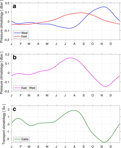
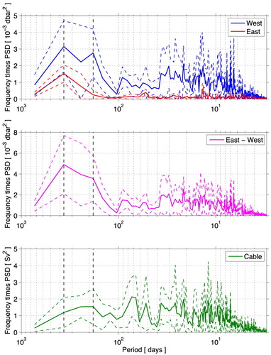
Figure 5. (a) Variance preserving spectra of the daily-averaged west and east pressure records. (b) Variance preserving spectrum of the pressure difference (east minus west). (c) Variance preserving spectrum of the Florida Current volume transport from the cable record during the coincident time period. All spectra were calculated using the Welch’s averaged periodogram method with a two-year window allowing one-year of overlap. Black vertical dashed lines highlight the annual and semi-annual periods. Dashed colored lines indicate the 95% confidence limits for the spectra.

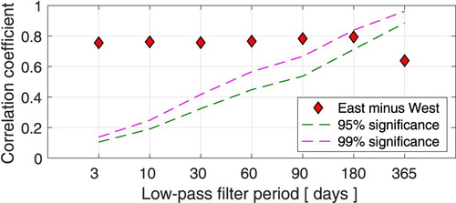
Further breakdowns of the records by time scale are helpful in comparing to the earlier results published by Maul et al. (1985, 1990). Given the earlier results showing that the daily negative west side pressure is less well correlated with the cable than is the pressure difference, it seems likely that further investigation with the negative west pressure is not warranted. Evaluating the correspondence between the pressure difference and cable daily time series based on time scale, however, is informative. The cable time series and the time series of pressure differences were each low-pass filtered (2nd order Butterworth, passed both forward and backward to avoid phase shifts) with cutoff periods of 3, 10, 30, 60, 90, 180, and 365 days, and the correlation between these pairs of filtered time series were compared to find the correlation coefficient r between the filtered records (Figure 6). For all periods less than annual, the correlation coefficient is essentially the same. At the annual period the correlation drops markedly, however the resulting correlation coefficient is not significantly different from zero given the length of the record. The lack of changes in the correlation for the records filtered with different cutoff periods suggests that for these pressure records collocated with the cable, there is not any sensitivity to the time scale being studied (i.e. up to annual periods).

Figure 6. Correlation coefficient r between Florida Current cable transport time series and the pressure difference (P_east – P_west). Correlation coefficient r is shown for the time series after they have been low-pass filtered with a 2nd order Butterworth filter, passed both forward and backward to avoid phase shifting, with the indicated cut-off periods. Also shown are the 95% and 99% significance levels for the correlation values based on the assumption that the integral time scales of the filtered time series are nominally equal to the filter cut-off period.

Ultimately, validation of the cable and/or the pressure difference methods of observing the Florida Current transport will come from comparison with independent data. Perhaps the most definitive test is to compare against quasi-instantaneous transports estimated from ship sections. Maul et al. (1985, 1990) compared their pressure data against repeated sections with a Pegasus velocity profiler (Spain et al. 1981). A similar approach is used herein, comparing both the pressure difference (P_east – P_west) and the cable observations to the ship section data for the period. Note that a few of the dropsonde cruises are not ‘fully independent’ from the cable data, in that they are used to test and adjust the calibration of the cable whenever the recording system is changed (e.g. Larsen 1992; Meinen et al. 2010). This calibration adjustment is only to the ‘constant’ of the linear calibration; the 24.42 Sv/volt ‘slope’ has remained the same since this telecommunication cable began use for monitoring the Florida Current in the 1990s. As such, the variability of the dropsonde cruises is fully independent of the cable data variability. A total of 33 dropsonde sections and 24 LADCP sections are available for this analysis (Figure 7). In order to compare the ship section data to the pressure gauge data, the pressure difference values must be ‘translated’ into an equivalent estimate of volume transport. For this comparison, the pressure differences have been ‘calibrated’ into the equivalent volume transport using a slope and intercept derived from a least-squares linear fit between the cable time series and the pressure differences (i.e. the non-normalized version of the time series shown in Figure 3(a)). By evaluating the scatter in the resulting comparisons with the ship section data, the ‘accuracy’ of using either the cable and/or the pressure differences can be determined (Figure 7). As is visually evident in Figure 7, the scatter of the ship section comparisons to the cable (red diamonds) is tighter than the scatter between the ship sections and the pressure differences (blue squares), a fact that is confirmed by the quantifying statistics (Table 3). The correlation and root-mean-squared (RMS) differences between the cable and the ship sections are much better than those between the pressure difference and the ship sections. The fact that the LADCP correlations are higher, for both cable and pressure difference, is likely a reflection of the smaller sample size, i.e. that there are roughly a third fewer LADCP cruises than dropsonde cruises. The RMS differences between the pressure difference transport estimates and the ship section estimates are nearly a factor of two larger than the RMS differences between the cable and the ship sections, for both the dropsonde cruises and the LADCP cruises. If one assumes that the errors in the pressure gauge difference method of estimating the transport are independent of the errors in the dropsonde measurements, which seems reasonable, then one can produce an estimated accuracy of the pressure gauge difference method as the square root of the observed RMS differences (2.8 Sv; see Table 3) squared minus the dropsonde accuracy (0.8 Sv; Garcia and Meinen 2014) squared. This gives an estimated accuracy for the daily Florida Current transport determined using the pressure gauge difference method of 2.7 Sv.

Figure 7. Comparison between direct estimates of Florida Current volume transport from ship sections to estimates of transport from the voltages measured on the cable (red diamonds) and to pressure differences (blue squares), where the pressure differences have been ‘calibrated’ into transport estimates simply by a least-squares fit of the daily pressure differences against the daily cable transports over the full period. Comparisons are shown for the 33 dropsonde sections (a) and the 24 LADCP sections (b) available during the time period overlapping with the pressure gauge data.

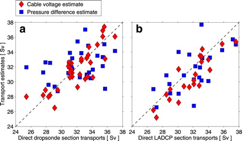
Table 3. Statistics of comparisons between direct measurements of Florida Current volume transport calculated from dropsonde or LADCP ship measurements and the simultaneous transport estimates from the cable or from the pressure differences calibrated into equivalent transport as discussed in the text.

Type of ship section	Number of sections	Comparison to cable		Comparison to pressure difference (Peast – Pwest)
		Correlation coefficient r	Root-mean-squared difference	Correlation coefficient r	Root-mean-squared difference
dropsonde	33	0.84	1.5 Sv	0.28	2.8 Sv
LADCP	24	0.94	1.7 Sv	0.72	2.6 Sv

Conclusions

The comparisons presented herein, utilizing two continuous tide gauge records located at arguably the ‘best possible’ locations for comparison with the cable measurements, indicate that paired tide gauges on either side of the Straits of Florida are a decent, but not perfect, solution for replacing the cable measurements. The correlation between the pressure difference between the tide gauges and the independent ship section-based transports is much lower, and the RMS difference between the transport observations is much higher, than for the corresponding comparisons with the cable measurements. This is not to say that the paired tide gauges are not valuable – they do appear to capture roughly half of the variance in the Florida Current transport at a wide range of time scales from a few days out to a year. Therefore, the paired tide gauges do represent a ‘much better than nothing’ option should the cable break at a future date. Clearly the tide gauge observations should be continued as a backup system to the cable.

The paired tide gauges are not, however, good enough alone. Further investigation is needed to determine what additional observations (e.g. altimetry, deep velocity) would be required to capture the remaining half of the variance that the tide gauges are missing. Previous analyses of the ship section data in the Straits have suggested that the near surface and near bottom flows are varying in an independent manner (e.g. Meinen et al. 2016). As such, it seems likely that additional observations of the deep flows within the Straits of Florida would be a necessary compliment to the near-surface tide gauges.

Acknowledgements

The authors would like to express their great appreciation to all of the scientific divers who have helped to maintain the pressure gauge moorings over the years, especially Grant Rawson, as well as to the ship captains and crews of the R/Vs F.G. Walton Smith, Endeavor, Seward Johnson, Knorr, Oceanus, and Atlantic Explorer, the NOAA Ship Ronald H. Brown, the RRS Discovery, and numerous small charter vessels for their outstanding support of the observational field program. The pressure gauges, ship section data (dropsonde and CTD/LADCP), and the cable observations have been supported by the U.S. NOAA Climate Program Office-Ocean Observing and Monitoring Division via the Western Boundary Time Series (WBTS) project (FundRef number 100007298) and by the U.S. NOAA Atlantic Oceanographic and Meteorological Laboratory. The authors received some support from the WBTS project and from the NOAA Atlantic Oceanographic and Meteorological Laboratory for this work. RFG was also supported in part under the auspices of the Cooperative Institute for Marine and Atmospheric Studies (CIMAS), a cooperative institute of the University of Miami and NOAA, cooperative agreement NA10OAR4320143. Shenfu Dong and an anonymous reviewer provided a number of helpful suggestions for improving earlier versions of the manuscript.

Data availability statement

The pressure/tide gauge data, the LADCP data, and the dropsonde data are available via the Western Boundary Time Series project web page at: www.aoml.noaa.gov/phod/wbts/. The Florida Current cable data are available at www.aoml.noaa.gov/phod/floridacurrent/.

Disclosure statement

No potential conflict of interest was reported by the author(s).

Additional information

Funding

This work was supported by National Oceanic and Atmospheric Administration: [Grant Number FundRef number 100007298].

References

- Church JA, White NJ. 2011. Sea-level rise from the late 19th to the early 21st century. Surv Geophys. 32:585–602. doi:10.1007/s10712-011-9119-1.
- Emery WJ, Thomson RE. 1997. Data analysis methods in physical oceanography. Oxford, UK: Pergamon. 638 pp.
- Garcia RF, Meinen CS. 2014. Accuracy of Florida Current volume transport measurements at 27°N using multiple observational techniques. J Atmos Ocean Tech. 31(5):1169–1180. doi:10.1175/JTECH-D-13-00148.1.
- Johns E, Wilson WD, Molinari RL. 1999. Direct observations of velocity and transport in the passages between the Intra-Americas Sea and the Atlantic Ocean, 1984–1996. J Geophys Res 104(C11):25805–25820. doi: 10.1029/1999JC900235
- Larsen JC. 1991. Transport measurements from in-service undersea telephone cables. IEEE J Oceanic Eng. 16(4):313–318. doi: 10.1109/48.90893
- Larsen JC. 1992. Transport and heat flux of the Florida Current at 27°N derived from cross-stream voltages and profiling data: theory and observations. Phil Trans R Soc Lond A. 338:169–236.
- Larsen JC, Sanford TB. 1985. Florida Current volume transports from voltage measurements. Science. 227:302–304. doi: 10.1126/science.227.4684.302
- Leaman KD, Vertes PS, Atkinson LP, Lee TN, Hamilton P, Waddell E. 1995. Transport, potential vorticity, and current/temperature structure across Northwest Providence and Santaren Channels and the Florida Current off Cay Sal Bank. J Geophys Res. 100(C5):8561–8569. doi: 10.1029/94JC01436
- Maul GA, Chew F, Bushnell M, Mayer DA. 1985. Sea level variation as an indicator of Florida Current volume transport: comparisons with direct measurements. Science. 227:304–307. doi: 10.1126/science.227.4684.304
- Maul GA, Mayer DA, Bushnell M. 1990. Statistical relationships between local sea level and weather with Florida-Bahamas cable and Pegasus measurements of Florida Current volume transport. J Geophys Res. 95(C3):3287–3296. doi: 10.1029/JC095iC03p03287
- Mayer DA, Leaman KD, Lee TN. 1984. Tidal Motions in the Florida Current. J Phys Oceanogr. 14:1551–1559. doi: 10.1175/1520-0485(1984)014<1551:TMITFC>2.0.CO;2
- McCarthy GD, Smeed DA, Johns WE, Frajka-Williams E, Moat BI, Rayner D, Baringer MO, Meinen CS, Collins J, Bryden HL. 2015. Measuring the Atlantic Meridional overturning circulation at 26°N. Prog Oceanogr. 130:91–111. doi: 10.1016/j.pocean.2014.10.006
- Meinen CS, Baringer MO, Garcia RF. 2010. Florida Current transport variability: an analysis of annual and longer-period signals. Deep Sea Res. I. 57:835–846. doi:10.1016/j.dsr.2010.04.001.
- Meinen CS, Luther DS. 2016. Structure, transport, and vertical coherence of the Gulf Stream from the Straits of Florida to the Southeast Newfoundland Ridge. Deep Sea Res. I. 111:16–17. doi:10.1016/j.dsr.2016.02.002.
- Montgomery RB. 1938. Fluctuations in monthly sea level on eastern U.S. coast as related to dynamics of western North Atlantic Ocean. J Mar Res. 1(2):165–185. doi: 10.1357/002224038806440584
- Mooers CNK, Meinen CS, Baringer MO, Bang I, Rhodes R, Barron CN, Bub F. 2005. Cross validating ocean prediction and monitoring systems. EOS (Washington, DC). 86(29):269, 272–273. doi:10.1029/2005EO290002.
- Niiler PP. 1968. On the internal tidal motions in the Florida Straits. Deep-Sea Res. 15:113–123.
- Pawlowicz R, Beardsley B, Lentz S. 2002. Classical tidal harmonic analysis including error estimates in MATLAB using t_tide. Comp Geosci. 28(8):929–937. doi:10.1016/S0098-3004(02)00013-4.
- Richardson WS, Finlen JR. 1967. The transport of Northwest Providence Channel. Deep Sea Res. 14:361–367.
- Sanford TB. 1982. Temperature transport and motional induction in the Florida Current. J Mar Res. 40(Suppl):621–639.
- Schott F, Zantopp R. 1985. Florida Current: seasonal and interannual variability. Science. 227(4684):308–311. doi: 10.1126/science.227.4684.308
- Smeed DA, Josey SA, Beaulieu C, Johns WE, Moat BI, Frajka-Williams E, Rayner D, Meinen CS, Baringer MO, Bryden HL, McCarthy GD. 2018. The North Atlantic Ocean is in a state of reduced overturning. Geophys Res Lett. 45:1527–1533. doi:10.1002/2017GL076350.
- Smith WHF, Sandwell DT. 1997. Global sea floor topography from satellite altimetry and ship depth soundings. Science. 277(5334):l956–1962. doi: 10.1126/science.277.5334.1956
- Spain PF, Dorson DL, Rossby HT. 1981. PEGASUS: a simple, acoustically tracked, velocity profiler. Deep Sea Res. 28:1553–1567. doi: 10.1016/0198-0149(81)90097-2
- Stommel H. 1948. The theory of the electric field induced in deep ocean currents. J Mar Res 7:386–392.
- Stommel H. 1957. Florida Straits transports: 1952–1956. Bull Mar Sci Gulf Carib. 7:252–254.
- Stommel H. 1959. Florida Straits transports: June 1956–July 1958. Bull Mar Sci Gulf Carib. 9:222–223.
- Stommel H. 1961. Florida Straits transports: July 1958–March 1959. Bull Mar Sci Gulf Carib. 11:318.
- Wertheim GK. 1954. Studies of the electric potential between Key West, Florida, and Havana, Cuba. Trans Am Geophys. U. 35:872–882. doi: 10.1029/TR035i006p00872
- Wunsch C, Hansen DV, Zetler BD. 1969. Fluctuations of the Florida Current inferred from sea level records. Deep-Sea Res. 16(Suppl.):447–470.
- Wunsch C, Wimbush M. 1977. Simultaneous pressure, velocity and temperature measurements in the Florida Straits. J Mar Res. 35:75–104.