Variational data assimilation of sea surface height into a regional storm surge model: Benefits and limitations

ABSTRACT

Storm surges are coastal sea-level variations caused by meteorological conditions. It is vital that they are forecasted accurately to reduce the potential for financial damage and loss of life. In this study, we investigate how effectively the variational assimilation of sparse sea level observations from tide gauges can be used for operational forecasting in the North Sea. Novel data assimilation ideas are considered and evaluated: a new shortest-path method for generating improved distance-based correlations in the presence of coastal boundaries and an adaptive error covariance model. An assimilation setup is validated by removing selections of tide gauges from the assimilation procedure for a North Sea case study. These experiments show widespread improvements in RMSE and correlations, reaching up to 16 cm and 0.7 (respectively) at some locations. Simulated forecast experiments show RMSE improvements of up to 5 cm for the first 24 h of forecasting, which is useful operationally. Beyond 24 h, improvements quickly diminish however. Using the setup based on the shortest path algorithm shows little difference when compared to a simpler Euclidean method at most locations. Analysis of this event shows that improvements due to data assimilation are bounded and relatively short lived.

1. Introduction

Coastal floods are a major hazard globally with severe economic and environmental consequences. In a world of changing climate and rising seas, the risk to coastal communities from storm surges is increasing (Bindoff et al. 2007; Haigh et al. 2010; Menendez and Woodworth, 2010; Church et al. 2013). Globally, the increase in extreme sea levels will result in critical flood defence thresholds being breached more frequently and therefore the risk of flooding will increase. Allowing for investment in adaptation measures (e.g. rising flood defences), global flood losses in 136 of the world's largest coastal cities have recently been estimated (Hallegate et al. 2013) to rise from US 6 billion per year in 2005 to US60–63 billion per year by 2050. For the European coastline, expected annual damages due to coastal flooding are projected to increase (Vousdoukas et al. 2018) by two to three orders of magnitude (from €1.25 billion today) by 2100. For the UK currently, $150 billion of assets and 4 million people are at risk from coastal flooding (Flowerdew et al. 2009). Jevrejeva et al. (2018) warn that without additional adaptation, the UK would be exposed to flood risk of 6.5% of UK GDP (800 billion per year) by 2100 if the worst greenhouse gas emissions scenario is realised. These drivers mean that vulnerable coastal communities will be at increased risk in the future. Forecasting models for waves and storm surges, delivery mechanisms and monitoring technologies therefore need to constantly innovate, in order to provide the state of the art warning systems needed by emergency responders to protect lives and livelihoods.

A storm surge is the regional increase in sea level due to passage of a storm and can last from hours to days and span hundreds of square kilometres. In European shelf seas, they can produce sea levels several metres higher than tides alone (Wadey et al. 2015). The primary mechanisms that contribute to the generation of a storm surge (Pugh and Woodworth, 2014) are:

1. The inverse barometer effect increases sea level due to local areas of low air pressure generating converging currents. This is the larger contribution away from the coast.

2. Momentum transfer from strong winds to the sea surface by wind setup drives water against coastal boundaries. This is the dominant mechanism in shallower coastal areas.

Other factors contributing to extreme sea levels are wave setup and superimposed wind waves which, when combined, lead to the overtopping of coastal defences. Additional dynamical considerations which affect sea levels are interactions between the surge, the tides and wave action (Horsburgh and Wilson, 2007; Wolf, 2008).

In the mid-latitudes, storm surges are created by extratropical cyclones. These are low-pressure atmospheric systems that are typically accompanied by strong winds and generally bad weather. Northwest Europe is a region particularly vulnerable to destructive storm surges due to areas of low lying land (e.g. The Netherlands and East Anglia) and shallow seas (Gonnert et al. 2001). A prominent example of such a surge occurred on the night of 31 January 1953 (Gerritsen, 2005). A large depression generated a storm surge in the North Sea that swept southwards along the UK coastline. The surge, which coincided with spring tides, resulted in hundreds of deaths (1836 in the Netherlands, 307 in the UK), as well as an estimated £50 million of damage in the UK. Partially as a response, many new coastal defences have been constructed and storm surge forecasting has made substantial improvements over the last three decades.

The benefits of improvements to forecasting and defences can be seen by contrasting the 1953 storm with the more recent ‘Xaver’ North Sea storm surge of 5–6 December 2013 (Sibley et al. 2015; Wadey et al. 2015). The strong winds that accompanied this event brought non-tidal residuals of up to 3.4 m and skew surges of up to 2 m in parts of the North Sea. In total, 1710 home were reported to have been flooded along the East coast of England, while thousands were evacuated throughout areas bordering the Irish and North Seas. Although this event was in many ways meteorologically similar to that of the 1953 event (similar depression and coincident surge and spring tides), the impacts were far less. The storm and surge resulted in significant damage to coastal structures and defences, flooded 2800 properties in the UK and damaged infrastructure (Wadey et al. 2015). Despite the reduced impacts, however, it is still one of the most damaging surge events in north-western Europe since the 1953 event.

Operational forecasting of storm surges is routinely performed using numerical hydrodynamical models. For instance, in the UK the Met Office provides storm surge and wave forecasts four times per day using an ensemble of the same depth-averaged hydrodynamical model that is used in this study (Flowerdew et al. 2009). Many operational tide-surge forecasting models use the depth-averaged Navier-Stokes equations for modelling sea surface height. The equations are often modelled using finite differencing on a choice of Arakawa grid (Messinger and Arakawa, 1976), although this can vary. Model domains are normally regional, allowing for a higher resolution, and are forced at the air–sea interface by the best resolution numerical weather prediction models. Operational systems serve national needs so there is an ongoing necessity to improve the accuracy of forecasts. One candidate to further improve the accuracy of storm surge models is data assimilation.

Data assimilation (DA) is used for estimating the true state of a system using multiple data sources. Typically, this involves combining model variables (background variables) with observations of the system, while taking into account information about errors in each. For forecasting applications, DA is typically used to create improved initial conditions for a model run or to update the model state at specific time steps. This is done to mitigate the propagation and amplification of model errors over time. Other applications include the creation of reanalysis datasets, where data from multiple sources are combined to generate an accurate as possible picture of the state of a system in the past. Such datasets can be useful for improving physical understanding and validation, for example see studies by Bresson et al. (2018) and Brown et al. (2010).

DA is integral for modern weather forecasting and has been used for decades (Lorenc, 1986; Daley, 1991). Weather forecasting agencies such as the Met Office, Meteo-France and the Canadian Meteorological Service all use it to initialise their forecast models (see for example Gauthier et al. 1999; Rawlins et al. 2007; Daniel et al. 2009). DA has also been used for ocean prediction. For example, Hoyer and She (2007) assimilated sea surface temperature observations from multiple sources, including satellites. It has also been shown to have operational benefit for ocean wave forecasting, see for example Voorrips (1999) and Almeida et al. (2015).

A limited amount of work has been done on using data assimilation in storm surge forecasting. In the North Sea, Madsen et al. (2015) looked at the assimilation of reconstructed altimetry data and successfully improved their model. However, their method involves the assimilation of large amounts of data, which is costly and time consuming. They also assimilated data only every 12 h. Zijl et al. (2015) used a Kalman filter to assimilate sea-level data into the North Sea sea-level forecasting, seeing improvements for the first few hours of forecast. Variational techniques have been little studied in storm surge forecasting: Lionello et al. (2006) did use variational assimilation for a forecasting model of the Adriatic Sea, however, only considered the assimilation of data from a single location and the system is no longer in use.

In this paper, we build on the above studies by evaluating the use of variational data assimilation of tide gauge data in operational storm surge forecasting in the North Sea and attempt to quantify its limitations. Tide gauge observations are easily accessible in real time and so any improvements due to their assimilation is of great practical use. We bring together ideas from atmospheric data assimilation as well as new ideas for dealing with the problems not present in the atmosphere such as coastal boundaries. A number of numerical experiments are performed, making use of a specific case study: the 2013 Xaver storm surge event.

2. Methods

In this paper, a data assimilation system has been created to work with observations from tide gauges and an operational storm surge forecasting model. This section describes in detail the model used, the data assimilation setup and the numerical experiments used to validate the system and evaluate forecasting skill. Two assimilation setups are considered: one using a traditional parametric covariance model and the other used a novel coast-following method, both of which are explained below.

2.1. Model

As potential improvements to operational storm surge forecasting is being evaluated, the CS3X (Continental Shelf Model 3) model is used as a numerical tool. This model has seen extensive use for operational storm surge forecasting around the UK by the UK Met Office from 1991 to 2020 and is one of the most validated operational storm surge models. At the time of writing, the UK Met Office was in the process of replacing CS3X with the NEMO model for future scalability and consistency with other systems. CS3X uses a grid with resolution $1/9^{\circ }$ (latitude) by $1/6^{\circ }$ (longitude) – a resolution of approximately 12 km. Its domain covers the area between ${40}^{\circ }\mathrm{N}$ to ${63}^{\circ }\mathrm{N}$ and ${20}^{\circ }\mathrm{W}$ to ${13}^{\circ }\mathrm{E}$. The sea surface is modelled using finite differencing of 2D depth-averaged Navier-Stokes equations. Three dimensional models may also be used for storm surge modelling and are especially useful where multi-directional flows, stratification and internal waves/tides are significant. However, these models require more computational resources but offer little improvement for operational forecasting skill, for example, see Bertin et al. (2012), Dangendorf et al. (2014), and Kodaira et al. (2016).

Tidal forcing is applied at the domain boundaries using the 26 largest constituents derived from a harmonic analysis of the NEA ocean model (Flather, 1980). This forcing is applied as elevations and currents. Tidal potential forcing is also applied to the whole domain, using equilibrium tide data as in Cartwright and Taylor (1971). Wind stress is parameterised from wind speed using the Charnock formulation (Charnock, 1955), where the surface drag coefficient $C_D$ is calculated from a surface roughness defined as: (1) $z_0=\frac{\alpha u_{\ast }^2}{g},$(1) where $u_{\ast }$ is friction velocity, g is gravity, and α is the Charnock parameter. A value of 0.0275 was found by Williams and Flather (2000) to optimise storm surge modelling in CS3X. The atmospheric forcing used at each timestep is derived from forecasted wind and sea-level pressure fields with a catenated 6-h lead time (UK Met Office Unified Model). Using these fields allows us to reduce errors introduced by inaccuracies in the atmospheric data and to isolate improvements to the ocean model alone.

2.2. Data assimilation setup and observations

2.2.1. Overview of assimilation scheme

A variational data assimilation scheme (VAR) is used for assimilation (Lorenc, 1986). Such schemes (e.g. 3DVar and 4DVar) have been used extensively and with success in Numerical Weather Prediction (NWP) (Andersson et al. 1998; Courtier et al. 1998; Rabier et al. 1998; Gauthier et al. 1999; Lorenc et al. 2000). 4DVar is the current standard (Klinker et al. 2000; Mahfouf and Rabier, 2000; Rabier et al. 2000; Gauthier et al. 2007; Rawlins et al. 2007) and is especially useful when observations are spread irregularly in time. State of the art methods include Ensemble 4DVar methods (Zhang et al. 2009; Buehner et al. 2010; Kuhl et al. 2013) and Ensemble Kalman Filter methods (Houtekamer and Mitchell, 2001; Houtekamer and Zhang, 2016). For the purpose of this study however, we neglect the time dimension and use 3DVar.

Variational assimilation requires the minimisation of a cost function: (2) $J(x)=\delta x^T{\mathbf{B}}^{-1}\delta x+(y-\mathbf{H}{x}_b{)}^T{\mathbf{R}}^{-1}(y-\mathbf{H}{x}_b),$(2) where $J(x)$ is the scalar cost function, $x_a$ is the analysis and the variable over which J is minimised, $x_b$ is the background state vector, y is the vector of observations, $\mathbf{H}$ is the observation operator, which transforms vectors of variables from the model grid space to the observation space, $\mathbf{B}$ is the matrix of covariances between the errors of background variables in the model grid space and $\mathbf{R}$ is the matrix of error covariances between observations. The term $\delta x=x_a-x_b$ is known as the increment and $y-\mathbf{H}{x}_b$ the innovation. The minimisation problem has been solved using the conjugate gradient method (see Hestenes and Stiefel, 1952) on a system preconditioned using the control variable transform (CVT) (Lorenc et al. 2000). This uses the substitution $u=B^{\frac{1}{2}}\delta x$ into Equation (2(2) $J(x)=\delta x^T{\mathbf{B}}^{-1}\delta x+(y-\mathbf{H}{x}_b{)}^T{\mathbf{R}}^{-1}(y-\mathbf{H}{x}_b),$(2) ), also eliminating the need to calculate $B^{-1}$.

Total water level (TWL) data from 15 research-quality tide gauges around the North Sea is assimilated into the model (see Figure 1). They are chosen according to data availability and quality during the December 2013 storm surge event. We choose to assimilate total water level rather than non-tidal residuals as these contain phase alterations to the tide, which can manifest as large unrealistic periodic signals (Horsburgh and Wilson, 2007). This also means that the calculation and subtraction of tides at each assimilation timestep is not required. The datum of assimilated data is adjusted to match that of the model sea surface by subtracting a 1-year mean from the data. Importantly, this level will also correspond to the mean level of the tidal forcing applied at the domain boundaries. Error variances at observation locations are assumed to be uncorrelated, meaning that the matrix $R$ is diagonal – simplifying calculations somewhat. Variances are estimated through the analysis of 1 year of data filtered using a high pass filter to remove tidal signals. At all gauges used, a standard deviation on the order of 0.01 m has been found.

Figure 1. The North Sea. Tide gauge locations used for assimilation in this study are indicated by orange squares, approximate location of amphidromic points (points of zero tidal range) by black crosses and the approximate progression of the tidal wave crest by the black dashed line. The entire CS3X model domain is shown on the top right.

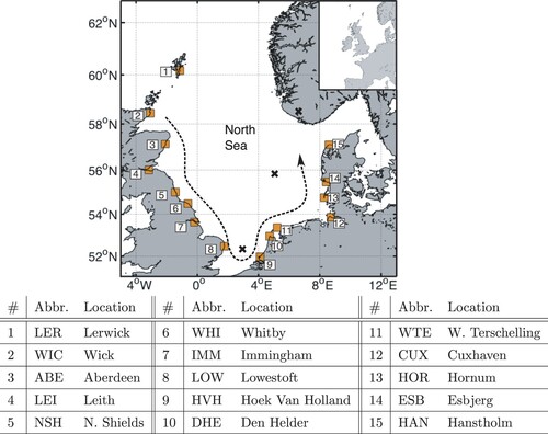
By assimilating total water level, corrections are not made only to the surge component of the model. The assimilated data contains part of the tidal signal, which will subsequently be introduced into the model analysis. Modelling shelf sea tides accurately remains challenging, therefore obtaining non-tidal residuals from the analysis (by subtracting a tide-only model run) becomes very difficult. To avoid this problem, our RMSE analysis in Section 3 is performed on TWL, not non-tidal residuals.

Information on barotropic currents is not assimilated into the model due to a lack of observations and cross correlations between variables are assumed to be zero. Instead, sea-level perturbations are introduced into the model using a short ramp function for stability. This function introduces sea-level increments gradually over a time window to reduce any shock to the model dynamics. This means that the $x$ and $y$ terms in Equation (2(2) $J(x)=\delta x^T{\mathbf{B}}^{-1}\delta x+(y-\mathbf{H}{x}_b{)}^T{\mathbf{R}}^{-1}(y-\mathbf{H}{x}_b),$(2) ) contain only sea-level information.

2.2.2. Covariance modelling

Two parametric background error covariance models have been developed using an analysis of innovation covariance, similar to Hollingsworth and Lonnberg (1986). Such models can be used to easily and cheaply create the background error covariance matrix $B$ in Equation (2(2) $J(x)=\delta x^T{\mathbf{B}}^{-1}\delta x+(y-\mathbf{H}{x}_b{)}^T{\mathbf{R}}^{-1}(y-\mathbf{H}{x}_b),$(2) ). Other methods, such as ensemble methods, are generally more costly to develop. Innovation-based methods for estimating the background error covariance work by substituting true background errors, which are unobtainable, with innovations. Assuming observation and background errors are uncorrelated then innovations covariances will match the background error covariance for points that are not collocated (Hollingsworth and Lonnberg, 1986). This does not hold as the separation between two points tends to zero, so other methods must be used to estimate the error variance. This is discussed further later in this section.

Tide gauge data is not used to calculate innovations as it is spatially sparse and limited to the coast. Instead reconstructed altimetry data developed by Hoyer and Andersen (2003) and Madsen et al. (2015) has been used from five periods in 2004-2006. This data were constructed by ‘blending’ together tide gauge and altimetry data to create dense sea-level datasets along altimetry tracks in the North Sea. It gives good spatial coverage both near the coast and in the interior. In doing this, the assumption is made that the error covariance is stationary in time (ergodic) since the experiments later in this study are performed for 2013 – a year for which the reconstructed dataset was not available.

The parametric covariance models use the distance between model point pairs as an independent parameter. The method used to calculate this distance is different for each covariance model. They are constructed in four steps, which are detailed further later in this section. These steps are:

(1)	Distances are determined between all background point-pairs.
(2)	Innovations are used to derive a parametric correlation function using distance as a parameter.
(3)	Innovations are used to estimate error variance for each background point and thus calculate the covariance.
(4)	The parametric covariance model is modified using the current state of the modelled sea surface using an adaptive localisation scheme.

Mathematically, the error covariance between any two background points i and j is constructed as follows: (3) $\mathbf{B}(i,j)={\sigma }_i{\sigma }_{j}P(i,j)\mathrm{\Phi }(i,j),$(3) where ${\sigma }_i$ and ${\sigma }_j$ are the estimated background error standard deviations at point i and j, respectively, $P(i,j)$ is an appropriate function of point-pair separation distance D and $\mathrm{\Phi }(i,j)$ is a localisation function that is dependent on the sea surface height at each point i and j. Each of these terms is described in more detail in the following sections.

Point-pair separation distance, D

As mentioned above, the separation distance D between any model point-pair is used as a parameter in the construction of the background error covariance matrix. Two distance calculation methods have been considered in this study: a Euclidean-based method and a shortest-path method. Often, for small domains, distance is calculated using a Euclidean-type or spherical method. Ocean signals propagate around coastal boundaries not through them; however, the straight line distance does not take this into account. Instead, a shortest path algorithm can be used to calculate distance and attempt to generate more realistic separation distances in a topographically complex domain. In this study, Dijkstra's algorithm (Dijkstra, 1959) has been used.

For more complex covariance estimation methods such as ensemble methods, the effects of along-coast covariance is accounted for intrinsically. Our method attempts to model this without the need for large computational resources and using a basic parametric covariance model.

Background error correlations, P

Error correlations between point pairs must be equal to 1 at zero distance and tend to zero at infinity and any function chosen to model correlations must reflect this (Gaspari and Cohn, 1999). In addition, the resulting correlation matrix must be positive definite, which is also a requirement for convergence of the conjugate gradient method used for the minimisation problem. To this end, a single-parameter exponential function is used: (4) $P(i,j)={\mathrm{e}}^{-\alpha D(i,j)},$(4) where $P(i,j)$ is the modelled correlation between background points i and j, $D(i,j)$ is their separation distance and α is some constant to be determined.

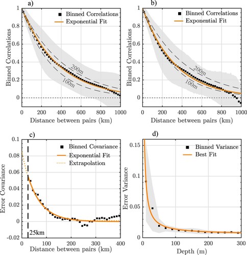
The analysis of innovations is used to determine the parameter α. Figure 2(a,b) shows innovation correlations binned by separation distance as well as the optimal fit for both the Euclidean and Dijkstra methods, both of which are good fits. The ideal shapes of a Kelvin wave according to the barotropic Rossby radius of deformation at ${55}^{\circ }\mathrm{N}$ for depths of 100 and 200 m are also shown. Both fits are of similar order to the the Rossby radius. Tides and storm surges in the North Sea propagate as coastally-trapped Kelvin waves and it appears that the errors behave in a similar fashion.

Figure 2. Model error statistics estimation. (a) and (b) show exponential fits to innovation correlations binned by distance according to the Euclidean and Dijkstra methods respectively. Grey dashed lines show the shape of a Kelvin wave according to the Rossby radius of deformation at ${55}^{\circ }\mathrm{N}$ for 100 and 200 m ocean depths. (c) An example of how variances were estimated for each individual background point. Innovation covariance is binned for distances over 25 km. An exponential fit is used to extrapolate to the y-axis (orange dashed line) to obtain a variance estimate. (d) Optimal fit to variance estimates binned by depth. In all cases, shading indicates one standard deviation either side of the mean.

Background error variance

Background error variances must also be approximated and parameterised for use in the covariance model. To do this, covariance is binned by distance for each background point where an innovation was available. An exponential function of the following form was then fitted for covariances at separation distances larger than 25 km: (5) $a_i{\mathrm{e}}^{-b_i{D}_{bin}},$(5) where $D_{bin}$ is is the distance used for binning, and $a_i$ and $b_i$ are constants to be determined by fitting individually for each point. We can use the variable a (the intercept with the y-axis) from each fit as a variance estimate. See Figure 2(c) for an example. As innovations are not available at all background points, we further parameterise variance by point-pair separation distance. This is done by fitting a final function of the following form to the above variance estimates: (6) ${\sigma }_i^2=\frac{m}{H_i}+n,$(6) where $H_i$ is the ocean depth at point i and m and n are constants to be determined by fitting. Variance was found to correlate well to a function of this form (see Figure 2(d)). Additionally, in shallower water and nearer the coasts, model errors are likely to increase quickly due to the relative influence of nonlinear effects. There is also a reciprocal relationship between the bottom friction terms in the barotropic equations of momentum and depth.

Figure 2(d) shows the variance estimates binned by ocean depth as well as the optimum function fit. At depths larger than $50m$, the error variance stays fairly uniform somewhere between 0.01 and 0.02. As the depth approaches zero, the variance increases rapidly, which is reminiscent of functions of the form seen in Equation (6(6) ${\sigma }_i^2=\frac{m}{H_i}+n,$(6) ). This could be explained by the increased influence of nonlinear effects and high sea level variability in areas closer to the coast.

Adaptive localisation

A secondary localisation step is also applied to the covariance model using a similar method to Riishøjgaard (1998). This is done via the elementwise multiplication of a correlation-like matrix, generated as a function of the difference in sea level between each point-pair. In other words, for two background points i and j, the function Φ can be defined as: (7) $\mathrm{\Phi }(i,j)=\mathrm{\Phi }(\Vert x_b(i)-x_b(j)\Vert ),$(7) where $x_b$ is the background variable as before and $\Vert X\Vert$ is the absolute value of X. If Φ is chosen such that the resulting matrix is positive definite, then an element-wise multiplication of our existing covariance matrix by the adaptive correlation matrix will result in a new positive definite covariance model (Riishøjgaard, 1998).

Due to the the difficulty of separating distance and sea level difference, we do not derive the adaptive component empirically. Instead we perform a set of tuning experiments to find an optimal paramter γ in an equation of similar form to Equation (4(4) $P(i,j)={\mathrm{e}}^{-\alpha D(i,j)},$(4) ): (8) $\mathrm{\Phi }(i,j)={\mathrm{e}}^{-\gamma \Vert x_b(i)-x_b(j)\Vert }.$(8) In reality, this tuning approach has no physical basis and would need to be performed independently for different regions and models. In preliminary tests, the inclusion of these adaptive correlations either improved or made no change to model accuracy at all locations. The effect of applying this step is to reduce covariances according to the dynamical state.

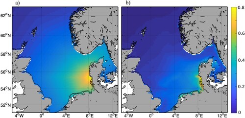
Figure 3 shows an example of how these covariances look for a single location both before and after the adaptive localisation is applied. In both cases shown, distances have been derived using the shortest path method. Before the localisation is applied, covariances clearly decrease monotonically with distance (which is expected). After this step, monotonicity is lost and sea level and bathymetric features can be seen, including Dogger Bank and the Norwegian Trench.

Figure 3. Map of background error covariance estimates at a single example timestep between Esbjerg and other model points. Panel (a) shows covariances for the parametric covariance model before the adaptive localisation step and (b) shows covariances after the adaptive localisation step. Both show the covariance model when calculating point-pair distances using a shortest path method.

2.3. Numerical experiments

This section describes the numerical experiments performed to validate the assimilation setup described above and to evaluate forecasting skill. The names and descriptions of the different experiments can be found in Table 1.

Table 1. Names and descriptions of the numerical experiments performed in this study.

Experiment name	Description
$V{A}_{LOC}$	Validation A. One by one, each tide gauge (indicated by LOC) is removed from the assimilation. RMSE and Correlations evaluated at LOC. Allows for maximum number of assimilated data as well as physical assessment.
$V{B}_{LOC}$	Validation B. Every other tide gauge assimilated starting at LOC, going anti-clockwise around North Sea.
$V{C}_{LOC}$	Validation C. Every third tide gauge assimilated starting at LOC, going anti-clockwise around North Sea.
SF	Simulated Forecasts. A period of assimilation at all locations (hindcast period) followed by a period of no assimilation (forecast period).
PT	Perturbation Test. 1m innovations assimilated one time at every gauge using a correlation function such that innovations are spread generously into the domain.

Note: LOC changes depending upon the specific model run.

For the validation runs (VA, VB and VC), a number of 120 h hindcasts have been performed for the time period 01/12/2013–05/12/2013, with hourly assimilation. To validate the assimilation setup, only a subset of the tide gauges shown Figure 1 are used in each run. Which gauges are included for each run are described in each Table 1. RMSE and correlations can then be assessed at the locations where data were not used for assimilation. This allows for an evaluation of how well the assimilation setup works with the model physics as well as how many locations are required for a good result.

A note on correlation calculation: as the tide is significant in the data, correlations are generally high. Therefore, correlations of non-tidal residuals are instead calculated. The results of our validation experiments are discussed in Section 3.1.

After validation, a set of simulated forecasts (SF) were run for the December 2013 Cyclone Xaver event (Wadey et al. 2015). These model runs were designed to simulate a realistic forecasting setup for this event and have been named to avoid confusion with real-time forecasts or hindcasts. Each simulated forecast is constructed to resemble a real operational scenario and consists of two parts: 120 h of hourly assimilation at all tide gauges up until some time T (hindcast period) followed by a period of no assimilation (forecast period). A separate simulated forecast has been performed for each location, timed such that T is 12 h before the maximum high water at that location. RMSE within a moving window is then evaluated during the forecast period. The results of our simulated forecast experiments are discussed in Section 3.2.

The final entry in Table 1 is the PT model run, which is used to determine how long SSH perturbations, such as those introduced by assimilation, persist in the model domain. This is discussed in more detail in Section 3.2.

3. Results and discussion

3.1. Validation of covariance models

Table 2 shows the averaged Root Mean Squared Error (RMSE) and correlations (compared to tide gauge observations) for each of the validation runs in Table 1. This table also indicates where there is improvement or deterioration of RMSE or where correlation improvements are significant. For RMSE, this is defined as 1 cm difference from the control (the observation error standard deviation estimated in Section 2.2). To compare correlations, a Fisher z-transformation is used (Fisher, 1915) with a 95% confidence interval. The values in these tables are metrics calculated over the tide gauges that were not included in the assimilation. So for the VA runs, this is at a single location, for VB runs it is over one half all locations and for the VC runs it is over two thirds of locations. Doing this allows us to assess how well our assimilation scheme can spread innovations into areas of the domain where observations are not available.

Table 2. Mean RMSE and correlations for the control model run alongside improvements in each.

RMSE (cm)	Control	Euc	Dijk	Corr	Control	Euc	Dijk
$V{A}_{Ler}$	7	0	0	$V{A}_{Ler}$	0.65	0.20	0.19
$V{A}_{Wic}$	21	5	5	$V{A}_{Wic}$	0.45	0.28	0.27
$V{A}_{Abe}$	11	1	0	$V{A}_{Abe}$	0.68	0.19	0.18
$V{A}_{Lei}$	31	13	13	$V{A}_{Lei}$	0.20	0.62	0.62
$V{A}_{Nsh}$	22	14	14	$V{A}_{Nsh}$	0.43	0.52	0.52
$V{A}_{Whi}$	15	9	9	$V{A}_{Whi}$	0.65	0.30	0.31
$V{A}_{Imm}$	22	3	2	$V{A}_{Imm}$	0.60	0.11	0.11
$V{A}_{Low}$	16	2	2	$V{A}_{Low}$	0.69	0.06	0.06
$V{A}_{Hvh}$	22	0	−1	$V{A}_{Hvh}$	0.67	−0.06	−0.08
$V{A}_{Dhe}$	33	9	10	$V{A}_{Dhe}$	0.49	0.32	0.33
$V{A}_{Wte}$	29	15	15	$V{A}_{Wte}$	0.58	0.33	0.33
$V{A}_{Cux}$	38	12	12	$V{A}_{Cux}$	0.60	0.26	0.26
$V{A}_{Hor}$	32	5	5	$V{A}_{Hor}$	0.61	0.13	0.13
$V{A}_{Esb}$	24	1	1	$V{A}_{Esb}$	0.75	−0.06	−0.06
$V{A}_{Han}$	21	4	5	$V{A}_{Han}$	0.91	−0.07	−0.05
$V{B}_{Ler}$	25	6	7	$V{B}_{Ler}$	0.55	0.25	0.26
$V{B}_{Wic}$	21	3	3	$V{B}_{Wic}$	0.64	0.16	0.16
$V{C}_{Ler}$	22	7	7	$V{C}_{Ler}$	0.64	0.21	0.21
$V{C}_{Wic}$	23	0	0	$V{C}_{Wic}$	0.61	0.04	0.04
$V{C}_{Abe}$	24	1	1	$V{C}_{Abe}$	0.55	0.06	0.06

Notes: This is shown for each validation run, using the Euclidean (Euc) and Djikstra (Dijk) covariance models (see Table 1). For the VA runs, the value is at a single location whereas for other runs they are averages across all non-assimilated locations. Positive values show improvement and negative values indicate deterioration. Bold text indicates significant improvement (over 1 cm or statistical significance), italics represents significant deterioration.

In general, there is little difference between the Euclidean and Dijkstra-based methods. This is likely due to regional considerations seeing as the North Sea is approximately a single rectangular basin (there are few significant headlands or peninsulas). For the VA model runs, most locations see improvements in RMSE and correlation for both covariance models. On average across removed locations, the VB validation runs show significant improvement over the control despite assimilating data from only eight locations. However, there is no significant improvement for 2 out of 3 of the VC validation runs.

The above results imply that if data is unavailable at certain gauges, the assimilation will still be reasonable until the distance between locations becomes too large. It is likely that this is related to number and proximity of tide gauges required to correctly resolve a tidal wavelength, which is in turn related to the Rossby radius. For example, the Rossby radius in the North Sea ranges between 200 and 300 km and the average distances between tide gauges for the VA, VB and VC validation runs are approximately 132, 232 and 328 km respectively. In other words, for the VC runs, the distance between observations exceeds the Rossby radius.

As a whole, these results suggest that our covariance models are reasonable estimations of the true error structure. The assimilation does more than just remove bias, it also improves the correlation between the model and observations.

3.2. Simulated forecasts: December 2013 case study

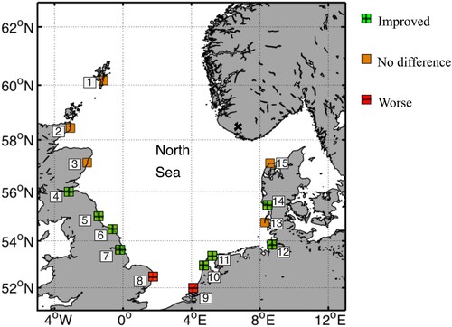
In this section, the results of the SF numerical experiments are discussed (see Table 1). These experiments were a set of model runs used to evaluate the models ability to forecast storm surges during the December 2013 Cyclone Xaver event. Figure 4 shows which locations saw a significantly improved or worsened RMSE during the first 24 h of forecast after the final assimilation time step. Results for both covariance models were near identical, therefore here we discuss results for both simultaneously. In total, 13 out of 15 locations see improvement or no significant change to RMSE during this time window and just over half (eight) see improvement. Two locations in the south see worsened RMSE. Again these are locations that are in close proximity to an amphidrome. On average across all locations, RMSE were improved by 0.02 m and the maximum improvement was 0.05 m. Although improvements are small, they are significant for operational applications.

Figure 4. Locations that saw improved, worsened or no significant difference to RMSE during the first 24 h of forecast from the simulated forecast model runs in this paper. Results from experiments using Euclidean and Dijkstra distances were near identical and this figure represents both. See Figure 1 for locations names.

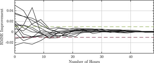
After the first 24 h of forecast, RMSE differences (and improvements) begin to diminish rapidly, becoming almost negligible by the end of second day. Figure 5 shows RMSE differences (from the control) calculated at each tide gauge location inside a moving 24 h window. Only results for the Dijkstra-based assimilation setup are shown. Where the lines intercept the y axis, the graph shows the mean RMSE difference during the first 24 h of forecast. The eight locations that saw RMSE improvement during the first 24 h period can be seen as the eight lines starting above the green dashed line. The shrinking RMSE differences can be seen clearly, with the vast majority of differences being within 0.01 m by the 12 h.

Figure 5. RMSE difference (relative to control) for a moving average RMSE (in total water level) with a window size of 24 h. The x-axis shows the number of hours since assimilation ended and the beginning of the RMSE window. Each line shows data for a different tide gauge. Positive indicates improvement and negative indicates worse RMSE values. Dashed lines indicate 0.01 m bounds. This is for the Dijkstra-based covariance model.

Correlations are more difficult to analyse for the forecast case. For a 24 h window, there are not enough data points to draw significant conclusions and for larger time windows, the differences are too small to be significant. During the first 24 h, there are only two significant differences (which are improvements) for each model run. After this, the same pattern of rapidly decreasing differences can be seen, as for RMSE.

These diminishing differences are due to the assimilated model rapidly tending back towards the control run. This is most likely because of the strong influence of boundary conditions on model dynamics. Tides enter the model at the domain boundaries, and when reaching the North Sea propagate in an approximately anti-clockwise direction (see Figure 1). Changes to the model sea surface (due to assimilation) also conform to this flow. The surge component of sea surface height is also strongly influenced by the atmospheric forcing, with which is strives to reach a dynamical balance. The above point is demonstrated further in the following section.

3.3. Persistence of assimilation increments

A simple numerical experiment has been performed to investigate how long assimilation increments persist in the model domain. For the PT model run (see Table 1), a deliberately unrealistic $1m$ innovation is assimilated into the model at all tide gauge locations. A non-adaptive correlation model is used in place of the full covariance models (i.e. the third and fourth steps outlined in Section 2.2.2 are not included when constructing the error covariance matrix). The outcome of this is that model increments will be large and spread widely across the domain. This is an extreme example but we use it solely to prove a point.

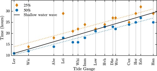
Figure 6 shows how many hours after assimilation it took for the final occurrence of a 0.5 and 0.25 m difference from the control run at each gauge. At Lerwick, we see the changes diminish to below 25% after a single tidal cycle. This time increases as one travels anti-clockwise around the North Sea; the same direction as the tidal flow. Except at a few locations (notably Leith), the increase is of the same order as the approximate time it takes for a shallow water wave to propagate in the same direction (also shown in Figure 6). Leith is the most obvious location that does not conform to this relationship. This may be because of its location inside a large estuary, where local oscillations such as seiching are more likely to be significant. Once introduced by the assimilation perturbation, these oscillations may continue independently of the tidal flow in the North Sea.

Figure 6. Number of hours taken for the differences due to an assimilation of a 1 m innovation at each tide gauge simultaneously to reduce to and never return to 50% and 25% of the original value. Tide gauges are spaced at distances from the previous tide gauge in an anti-clockwise direction (see Figure 1). Also shown is the distance travelled by a shallow water wave for a depth of 98 m (the mean depth of the model North Sea).

These results place an upper bound on the effectiveness of data assimilation in regional ocean models that are strongly constrained by surface and lateral boundary conditions and simple descriptions of frictional dissipation. As seen in Figure 5, increments do not last long anywhere in the system, likely due to the small domain size and proximity to unchanged boundary conditions. Having said this, it appears DA will have more of a prolonged effect in the Southeast of the sea than, for example, along the UK coastline. Unlike the atmosphere, it appears as though this type of ocean model does not display chaotic behaviour, again due to the strong dependence of the model upon boundary conditions.

4. Conclusions

In this study, the assimilation of tide gauge data into a North Sea storm surge model was investigated to examine how effectively it can be used to improve storm surge forecasting and coastal flooding risk assessment. To do this, two different data assimilation setups were developed and tested by performing validation hindcasts and simulated forecasts of the December 2013 Cyclone Xaver storm surge event. Another model run was done to quantify how long sea surface perturbations due to assimilation last in the model domain.

The covariance models necessary for variational assimilation were created in four steps. First, two different methods for calculating distances between model point-pairs were considered: a Euclidean method and a method based on Dijkstra's shortest path algorithm. Innovations and their spatial correlations were then calculated using reconstructed altimetry data, and an optimal exponential fit was used as a parametric correlation model. A similar method was then used to estimate model error variances based on ocean depth. Finally, an adaptive localisation component was added to the covariance model, based on the difference in sea level between model point-pairs.

Background error covariance was found to have a similar correlation length scale as the model physics themselves, i.e. on the same order as an average Rossby radius in the North Sea. Variances were small and uniform (around 0.02 m) for depths deeper than 50 m but increased rapidly for shallower depths. This makes sense as more complex nonlinear effects come into play in shallower, coastal seas. Ocean variability itself is higher in these areas, again suggesting that the errors behave in a similar way to the model dynamics. This supports the need for an adaptive component in the covariance model.

To validate the covariance models and assimilation setup, a set of 120 h validation experiments was performed, each with varying numbers of tide gauges removed from the assimilation (see Table 1 for model names). How well the assimilation setup performed was then examined by comparing the model to observations from locations that had not been assimilated into the model. Both covariance models performed well, with improvements in RMSE and correlations at most locations when compared compared to a control run with no assimilation. There was little difference between the Euclidean and Dijkstra methods, probably due to the shape of the North Sea, which is near to being mathematically convex. However, we believe this method to be worthy of further examination in more topographically complex domains.

From the validation experiments, it could be seen that operational significant improvements can still be obtained when assimilating data from only every other tide gauge (VB validation runs). However, once the distance between tide gauges extends beyond this, very little improvement can be obtained at other locations. The consequence of this for a real-time scenario is that if data is unavailable for a handful of locations (e.g. bad quality data, damaged equipment) then assimilation is still viable, at least whilst the distance between locations is less than approximately a Rossby radius of deformation.

Simulated forecasts of the December 2013 North Sea storm surge event showed that, although there was initially some small improvements, any RMSE differences quickly diminished. This was due to the assimilative models rapidly tending back to the control after assimilation was finished. We suggest that this is because of the ocean models reliance on boundary conditions, especially tidal and atmospheric forcing. This places an upper bound on the effectiveness of storm surge forecasting in the North Sea. Even with a perfect covariance model and assimilation scheme, significant adjustments to the model only persist for 12–24 h of forecast (along the UK coast). Furthermore, the DA would be a vital tool in any long storm surge reanalysis, e.g. to detect climatic trends or provide statistics for coastal planning.

Despite this, there are many avenues available for investigation to potentially improve the covariance model. The assumption of ergodic error correlations could be relaxed and more investigation made into how they vary with, for example, the seasons or with climate modes. More complex adaptive covariance models could also be developed, such as a reliance on current speed and direction as well as sea level height. Bespoke dynamical covariance models that optimise operational forecasting can also be conceived. For instance, if particular ports, cities or regions are particularly exposed to risks then the fact that all assimilated information travels at shallow water wave speeds allows for a dynamical adjustment of the covariance matrices focused on the subdomains with most influence on the solution at a later time. These could be identified by adjoint methods (Wilson et al. 2013).

The above bounds may limit the use of the assimilation for longer term forecasts. However, during the first 24 h of forecast (and thus during the surge event), the majority of locations saw some improvement in their RMSE values when using the adaptive covariance model. In some cases, this improvement was as high as 4–5 cm which can be significant for forecasting. Improvements of this size will improve confidence in the overall short term forecast, providing forecasters with the ability to give authoritative advice with fewer caveats regarding model performance. Although this timeframe is short, it is enough to warn the public of an event in advance with sufficient time to enable the targeted deployment of emergency responders.

This study has three important limitations which must be kept in mind when interpreting conclusions and results. Firstly, only a single case study was examined which is particularly pertinent when considering metrics such as RMSE and correlations. The values presented in this paper are examples to demonstrate potential improvements and the limitations of assimilation algorithms used. For statistically significant estimates of these metrics – which would be necessary for operational applications – further study of longer time periods and more events is required.

Secondly, it should be noted that the variational assimilation algorithm (2DVar) used is not state of the art, nor was it intended to be. Instead, the method used in this paper was chosen to demonstrate potential improvements from a low-cost method. Where resources are available, further work to examine more up to date methods such as ensemble 4DVar (Zhang et al. 2009; Buehner et al. 2010; Kuhl et al. 2013) or Ensemble Kalman filter methods (Houtekamer and Mitchell, 2001; Houtekamer and Zhang, 2016) is recommended.

The third and final limitation that must be noted is that by assimilating the full total water level signal, the tidal signal is not removed from either the observations or the model prior to assimilation. This will affect both the assimilation and resulting RMSE values from the model, with model corrections including components of both the storm surge and tidal signal. Indeed, many assimilative oceanographic systems such as those utilising altimetry data do not assimilate the full tidal signal. Which method is best will depend on the exact model, configuration and circumstance and requires further study.

Despite the above limitations, many of the conclusions in this study are applicable to the model behaviour itself and therefore offer insight for assimilation into similar regional models which are subject to strong boundary constraints.

Finally, a comparison can be made to other operational applications of data assimilation. For atmospheric forecasting (for example) there are more observations, the domains are larger and better connected (no coastal boundaries) and the models deal with far more variable interactions (Klinker et al. 2000; Mahfouf and Rabier, 2000; Rabier et al. 2000; Gauthier et al. 2007; Rawlins et al. 2007). As a result, there is less dependence upon the boundary conditions and perturbations to the model state persist for longer. The effects of chaos are more prevalent in the atmosphere than in semi enclosed seas such as the North Sea, which are heavily influenced by boundary conditions.

Acknowledgments

The research presented in this paper was supported by the Natural Environment Research Council's Understanding the Earth, Atmosphere and Ocean Doctoral Training Program (NE/L002469/1). The authors would like to thank Dr Andy Saulter of the UK Met Office, whose advice on the potential impacts of this work has been invaluable. Also thanks to Kristine S. Madsen and Jacob L. Hoyer of DMI for use of their blended tide gauge-altimetry sea-level datasets. UK tide gauge data were acquired from the British Oceanographic Data Centre (https://www.bodc.ac.uk/data/), Dutch data from Rijkswaterstaat (https://www.rijkswaterstaat.nl/), Danish data from the Dutch Meteorological Institute (https://www.dmi.dk/) and German data from the University of Hawaii Sea Level Center (https://uhslc.soest.hawaii.edu/). The regional storm surge model used throughout (CS3X) was used with permission from the National Oceanography Centre.

Disclosure statement

No potential conflict of interest was reported by the author(s).

Additional information

Funding

The research presented in this paper was supported by the Natural Environment Research Council's Understanding the Earth, Atmosphere and Ocean Doctoral Training Program [grant number NE/L002469/1].

References

- Almeida S, Rusu L, Soares CG. 2015. Data assimilation with ensemble Kalman filter in a high-resolution wave forecasting model for coastal areas. J Oper Oceanogr. 9(2):103–114.
- Andersson E, Haseler J, Undén P, Courtier P, Kelly G, Vasiljevic D, Brankovic C, Cardinali C, Gaffard C, Hollingsworth A, et al. 1998. The ECMWF implementation of three-dimensional variational assimilation (3D-Var). III: experimental results. Q J R Meteorol Soc. 124:1831–1860.
- Bertin X, Bruneau N, Breilh J-F, Forunato AB, Karpytchev M. 2012. Importance of wave age and resonance in storm surges: the case xynthia, bay of biscay. Ocean Model. 42:16–30.
- Bindoff N, Willebrand J, Artale V, Cazenave A, Gregory J, Guley S, Hanawa K, Levitus S, Nojiri Y, Shum C, et al. 2007. Observations: oceanic climate change and sea level. Cambridge, UK: Cambridge University Press. Book Section 5, p. 385–432.
- Bresson E, Arbogast P, Aouf L, Paradis D, Kortcheva A, Bogatchev A, Galabov V, Dimitrova M, Morvan G, Ohl P, et al. 2018. On the improvement of wave and storm surge hindcasts by downscaled atmospheric forcing: application to historical storms. Nat Hazards Earth Syst Sci. 18(4):997–1012.
- Brown JM, Souza AJ, Wolf J. 2010. An investigation of recent decadal-scale storm events in the Eastern Irish sea. J Geophys Res Oceans. 115:C05018.
- Buehner M, Houtekamer P, Charette C, Mitchell HL, He B. 2010. Intercomparison of variational data assimilation and the ensemble Kalman filter for global deterministic NWP. Part I: description and single-observation experiments. Mon Weather Rev. 138(5):1550–1556.
- Cartwright DE, Taylor RJ. 1971. New computations of the tide-generating potential. Geophys J R Astr Soc. 23:45–74.
- Charnock H. 1955. Wind stress on a water surface. Q J R Meteorol Soc. 81:639–640.
- Church JA, Clark PU, Cazenave A, Gregory JM, Jevrejeva S, Levermann A, Merrifield MA, Milne GA, Nerem RS, Nunn PD, et al. 2013. Sea level change. climate change 2013: the physical science basis. Contribution of working group I to the fifth assessment report of the intergovernmental panel on climate change. Cambridge, UK and New York, NY: Cambridge University Press.
- Courtier P, Andersson E, Heckley W, Pailleux J, Vasiljevic D, Hamrud M, Hollingsworth A, Rabier F, Fisher M. 1998. The ECMWF implementation of three-dimensional variational assimilation (3D-Var). I: formulation. Q J R Meteorol Soc. 1783–1807.
- Daley R. 1991. Atmospheric data analysis. Cambridge: Cambridge University Press.
- Dangendorf S, Müller-Navarra S, Jensen J, Schenk F, Wahl T, Weisse R. 2014. North sea storminess from a novel storm surge record since ad 1843. J Clim. 31(23):3582–3595.
- Daniel P, Haie B, Aubail X. 2009. Operational forecasting of tropical cyclones storm surges at Meteo-France. Mar Geodesy. 32(2):233–242.
- Dijkstra EW. 1959. A note on two problems in connexion with graphs. Numer Math. 1(1):269–271.
- Fisher RA. 1915. Frequency distribution of the values of the correlation coefficient in samples of an indefinitely large population. Biometrika. 10(4):507–521.
- Flather RA. 1980. Results from a model of the north east Atlantic relating to the Norwegian coastal current. Norwegian Coastal Current. 2:427–458.
- Flowerdew J, Horsburgh K, Wilson C, Mylne K. 2009. Flooding in England: a national assessment of flood risk. Environment agency report. J R Meteorol Soc. 136(651).
- Gaspari G, Cohn SE. 1999. Construction of correlation functions in two and three dimensions. Q J R Meteorol Soc. 125(554):723–757.
- Gauthier P, Charette C, Fillion L, Koclas P, Laroche S. 1999. Implementation of a 3D variational data assimilation system at the Canadian meteorological centre. part I: the global analysis. Atmos-Ocean. 37:103–156.
- Gauthier P, Tanguay M, Laroche S, Pellerin S. 2007. Extension of 3DVar to 4DVar: implementation of 4DVar at the meteorological service of Canada. Amer Meteorol Soc. 135:2339–2354.
- Gerritsen H. 2005. What happened in 1953? The big flood in the Netherlands in retrospect. Phil Trans R Soc. 363:1271–1291.
- Gonnert G, Dube SK, Murty T, Siefert W. 2001. Global storm surges: theory, observations and applications. Holstein, Die Kueste.
- Haigh I, Nicholls R, Wells N. 2010. Assessing changes in extreme sea levels: application to the english channel. Cont Shelf Res. 30:1042–1055.
- Hallegate S, Green C, Nicholls RJ, Corfee-Morlot J. 2013. Future flood losses in major coastal cities. Nat Clim Chang. 3:802–806.
- Hestenes MR, Stiefel E. 1952. Methods of conjugate gradients for solving linear systems. J Res Natl Bur Stand (1934). 49(6):409–436.
- Hollingsworth A, Lonnberg P. 1986. The statistical structure of short-range forecast errors as determined from radiosonde data. Part I: the wind field. Tellus. 38A:111–136.
- Horsburgh K, Wilson C. 2007. Tide-surge interaction and its role in the distribution of surge residuals in the North Sea. J Geophys Res. 112(C08003).
- Houtekamer PL, Mitchell HL. 2001. A sequential ensemble Kalman filter for atmospheric data assimilation. Mon Weather Rev. 129:123–137.
- Houtekamer PL, Zhang F. 2016. Review of the ensemble Kalman filter for atmospheric data assimilation. Mon Weather Rev. 144:4489–4525.
- Hoyer JL, Andersen OB. 2003. Improved description of sea level in the North Sea. J Geophys Res. 108(C5, 3136).
- Hoyer JL, She J. 2007. Optimal interpolation of sea surface temperature for the North Sea and baltic sea. J Mar Syst. 65:176–189.
- Jevrejeva S, Jackson LP, Grinsted A, Lincke D, Marzeion B. 2018. Flood damage costs under the sea level rise with warming of 1.5∘C and 2∘C. Environ Res Lett. 13:074014.
- Klinker E, Rabier F, Kelly G, Mahfouf J-F. 2000. The ECMWF operational implementation of four-dimensional variational assimilation. part III: experimental results and diagnostics with operational configuration. Q J R Meteorol Soc. 126:1191–1215.
- Kodaira T, Thompson KR, Bernier NB. 2016. The effect of density stratification on the prediction of global storm surges. Ocean Dyn. 66:1733–1743.
- Kuhl DD, Rosmond TE, Bishop CH, McLay J, Baker NL. 2013. Comparison of hybrid ensemble/4DVar and 4DVar within the NAVDAS-AR data assimilation framework. Mon Weather Rev. 141(8):2740–2758.
- Lionello P, Sanna A, Elvini E, Mufato R. 2006. A data assimilation procedure for operational prediction of storm surge in the Northern adriatic sea. Cont Shelf Res. 26(4):539–553.
- Lorenc AC. 1986. Analysis methods for numerical weather prediction. Q J R Meteorol Soc. 112:1177–1194.
- Lorenc AC, Ballard SP, Bell RS, Ingleby NB, Andrews PLF, Barker DM, Bray JR, Clayton AM, Dalby T, Li D, et al. 2000. The met office global three-dimensional variational data assimilation scheme. Q J R Meteorol Soc. 126(570):2991–3012.
- Madsen KS, Hoyer JL, Fu W, Donlon C. 2015. Blending of satellite and tide gauge sea level observations and its assimilation in a storm surge model of the North Sea and baltic sea. J Geophys Res. 120:6405–6418.
- Mahfouf J, Rabier F. 2000. The ECMWF operational implementation of four-dimensional variational assimilation. Part II: experimental results with improved physics. Q J R Meteorol Soc. 1171–1190.
- Menendez M, Woodworth PL. 2010. Changes in extreme high water levels based on a quasi-global tide-gauge data set. J Geophys Res. 115:15pp.
- Messinger F, Arakawa A. 1976. Numerical methods used in atmospheric models. Geneva: Atmospheric Research Programme WMO-ICSU Joint Organizing Committee GARP Publication Series.
- Pugh D, Woodworth P. 2014. Sea level science: understanding tides, surges, tsunamis and mean sea-level changes. Cambridge: Cambridge University Press.
- Rabier F, Jarvinen H, Kinkler E, Mahfouf J, Simmons A. 2000. The ECMWF operational implementation of four-dimensional variational assimilation. Part I: experimental results with simplified physics. Q J R Meteorol Soc. 126:1143–1170.
- Rabier F, McNally A, Andersson E, Courtier P, Unden P, Eyre J, Hollingsworth A, Bouttier F. 1998. The ECMWF implementation of three-dimensional variational assimilation (3D-Var). II: structure functions. Q J R Meteorol Soc. 124(550):1809–1829.
- Rawlins F, Ballard SP, Bovis KJ, Clayton AM, Li D, Inverarity GW, Lorenc AC, Payne TJ. 2007. The met office global four-dimensional variational data assimilation scheme. Q J R Meteorol Soc. 133:347–362.
- Riishøjgaard LP. 1998. A direct way of specifying flow-dependent background error correlations for meteorological analysis systems. Tellus. 50A:42–57.
- Sibley A, Cox D, Titley H. 2015. Coastal flooding in England and wales from Atlantic and North Sea storms during the 2013/2014 winter. Weather. 70(2):62–71.
- Voorrips C. 1999. Spectral wave data assimilation for the prediction of waves in the North Sea. Coastal Eng. 37:455–469.
- Vousdoukas MI, Mentaschi L, VoUKouvalas E, Verlaan M, Jevrejeva S, Jackson LP, Feyen L. 2018. Global probabilistic projections of extreme sea levels show intensification of coastal flood hazard. Nat Commun. 9:2360.
- Wadey MP, Brown JM, Haigh ID, Dolphin T, Wisse P. 2015. Assessment and comparison of extreme sea levels and waves during the 2013/14 storm season in two UK coastal regions. Nat Hazards Earth Syst Sci. 15(10):2209–2225.
- Williams JA, Flather RA. 2000. Interfacing the operational storm surge model to a new mesoscale atmospheric model. Proudman Oceanographic Laboratory [now National Oceanography Centre]. Technical Report: 127.
- Wilson C, Horsburgh K, Williams J, Flowerdew J, Zanna L. 2013. Tide-surge adjoint modelling: a new technique to understand forecast uncertainty. J Geophys Res. 118:5092–5108.
- Wolf J. 2008. Coastal flooding: impacts of coupled wave-surge-tide models. Nat Hazards. 49:241–260.
- Zhang F, Zhang M, Hansen JA. 2009. Coupling ensemble Kalman filter with four-dimensional variational data assimilation. Adv Atmos Sci. 26:1–8.
- Zijl F, Sumihar J, Verlaan M. 2015. Application of data assimilation for improved operational water level. Ocean Dyn. 65(12):1699–1716.