Creation of a global tide analysis dataset: Application of NEMO and an offline objective analysis scheme

ABSTRACT

The accurate prediction of tides is vital for the operation of many industries, early warning of coastal flooding and scientific understanding of ocean processes. In this paper, we describe the creation method of a global dataset of tidal harmonics using NEMO (Nucleus for European Modelling of the Ocean) for the first time and an offline objective analysis scheme. Data are assimilated as part of a post-processing step, reducing the computational resources required. A reduced ensemble of tidal harmonics is generated, where each member is run for a shorter period of time than a central background state. This ensemble is used to estimate a single background covariance state, which is used for analysis. Output is validated using an ensemble of objective analyses. For each ensemble member, random selections of observations are omitted and validation is performed at these locations. Improvements in both Mean Absolute Error (MAE) and correlation coefficients ($R^2$) are seen across all 6 of the largest diurnal and semi-diurnal constituents. MAEs in amplitude and phase are reduced by up to $78\text{\%}$ and $89\text{\%}$, respectively, and correlations by as much as 0.14. In addition, the majority of locations (between 70 and 80%) see significant improvement.

1. Introduction

Tides in the ocean are periodic movements due to the interactions of the Earth, Sun and Moon system (Pugh and Woodworth, 2014), often manifesting at the coast as a once or twice daily approach and recession of the ocean. Their prediction has a long history and many applications, both practical and scientific. They are vital for port operations, where ships and cargo must safely manoeuvre waterways and harbours. Forecasts of storm surges and resulting coastal inundation, such as those made by agencies such as the UK Met Office, rely heavily upon them, especially in regions with large tidal ranges. Whether or not the tide is high or low can make the difference between unnoticed changes in sea level and life-threatening coastal flooding. Commercial ocean operations such as oil drilling and coastal engineering also require accurate predictions as part of their working procedure.

Where there are long time series of observations available, such as at a tide gauge, tidal predictions may be created with relative ease using a harmonic analysis (Foreman and Neufeld, 1991; Foreman, 1996; Pugh and Woodworth, 2014). This procedure takes advantage of the strong periodicity in the tidal signal and decomposes it into the amplitudes and phases of its sinusoidal components, known as tidal constituents. Amplitudes and phases can then be used to reconstruct a tidal time series into the future with high accuracy. However, such methods are constrained by the availability of observations, both in time and space. Tidal predictions may only be made at the same location where the tidal signal was originally observed and in many regions, appropriate observations are sparse or none existent. Additionally, a long enough observed time series, at the appropriate frequency, is required in order to adequately resolve some constituents. In areas where observations are lacking, numerical models can instead be used to generate harmonics and subsequent predictions. Such models may be prone to errors, however. More accurate ‘analysis’ datasets can be developed through the use of data assimilation techniques to combine model data with observations.

The creation of global datasets of tidal harmonics using numerical models, data assimilation and inverse methods has been well studied (Pekeris and Accad, 1969; Schwiderski, 1979; Parke and Hendershott, 1980; Ray, 1999; Egbert and Bennett, 1996; Arbic et al., 2010). Prominent examples of existing up to date databases include TPXO9 (Egbert and Erofeeva, 2002), FES2014 (Carrere et al., 2016) and HAM12 (Taguchi et al., 2014). Stammer et al. (2014) give a comprehensive review of global tide datasets and their accuracy. These datasets contain varying numbers of harmonics based on the assimilation of a variety of observations into a numerical model.

In this paper, we investigate a lightweight methodology for the generation of a new assimilative global dataset of tidal harmonics at a $\frac{1}{12}$-degree resolution. The dataset is created via the combination of harmonic output from a numerical model and observations from bottom pressure recorders and tide gauges. For the first time, the NEMO (Nucleus for European Modelling of the Ocean (Madec, 2008)) model is used for this purpose. Data assimilation is performed as a post-processing routine rather than during the model simulation. Such a method is flexible enough to allow for the dataset to be updated whenever new harmonic data becomes available, without the need to run new simulations. A reduced ensemble approach is used, wherein an ensemble of model harmonics is used to generate a single covariance matrix, which is subsequently used for assimilation of observations into a single, long model run. This is a quicker and more lightweight approach than in standard ensemble routines.

In the following sections, the generation and validation of the dataset are detailed and discussed. In Section 2, all aspects of the generation of our data are described, including the numerical model configuration, the analysis scheme used, selection of observations and harmonic analyses. Following on from this in Section 3, an attempt is made to validate the analysis through the creation of a pseudo-analysis. Such a validation is necessary to give us confidence that the analysis scheme works. In this section, our dataset is also compared visually to another prominent global tide dataset.

2. Methods

2.1. Overview

The dataset discussed in this study is generated by combining harmonic output from a numerical model and observations using data assimilation techniques. The order of operations used to do this is as follows:

(1)	Run a numerical global ocean model to obtain fields of sea surface height (SSH).
(2)	Analyse model output to obtain fields of harmonic amplitudes and phases.
(3)	Select and analyse observations to obtain harmonic amplitudes and phases.
(4)	Combine the observed harmonics and model harmonics using an ensemble optimal interpolation scheme (OI).

In this section, details on each aspect of the dataset generation are given: the choice of numerical model, the data used, the assimilation scheme and decisions on harmonic analysis. There are number of datasets discussed in this study. For later reference, their names and descriptions may be found in Table 1.

Table 1. Reference table for names and descriptions of the datasets discussed in this study.

Name	Description
Raw model	Unadjusted harmonic output from the NEMO model. Bottom friction and SAL parameters are chosen to be at the centre of the values used for the ensemble.
Linearly adjusted model	Raw model harmonic that has been linearly adjusted such that errors contain no offset and no trend. This is used as the background variable for assimilation.
Analysis	Blending together of linearly adjusted model and all observations using data assimilation techniques. Also referred to in this paper as GTM
Validation analysis	Harmonic dataset derived from an ensemble of analyses. Each member is an analysis for which a random $\frac{1}{3}$ of observations is omitted from the assimilation procedure. Dataset is created by taking the ensemble average, but only when locations were omitted.
Observations	Harmonic observations from tide gauges and bottom pressure recorders used for assimilation and validation.

2.2. Numerical model

Background fields (see Section 2.4) are generated using a harmonic analysis of sea surface height (SSH) output from a numerical model, specifically NEMO (Nucleus for European Modelling of the Ocean) (Madec, 2008). The configuration used is similar to GO6 (Storkey et al., 2018), with a 1/12-degree ORCA Arakawa-C grid (Madec and Imbard, 1996) over a global domain. The grid is curvilinear and tripolar, allowing for the whole globe to be modelled. Physics are modelled using a finite difference integration scheme over 10 terrain-following vertical levels to resolve depth varying currents. Self-attraction and loading (see Farrell (1973) and Ray (1998)) are modelled using a scalar approximation scheme such that suggested by Accad and Pekeris (1978), with $\beta =0.94$. Tidal forcing is applied barotropically to the ocean as a pressure-like force. This forcing is determined from an estimation of the equilibrium tide amplitude and phase for each constituent, based on work by Cartwright and Taylor (1971). A set of 31 constituents are used for this purpose (henceforth ‘forcing’ constituents).

In all model runs, the ocean-free surface and currents begin at rest. Temperature and salinity are included in the model but are initially the same everywhere. All temperature and salinity fluxes into the ocean are set to zero for the duration of each run, keeping these variables constant. This homogeneity and constant density means that internal waves will not be well (or at all) represented by the model. However, the dissipation of barotropic tidal energy due to internal wave drag has been shown to be important in the open ocean (Egbert and Ray, 2000) and therefore must be parameterised in our configuration. This dissipation is modelled using the scale relation suggested by Jayne and Laurent (2001). The NEMO code was modified for this study to allow for this scheme. The modelling of ice is omitted from this version of the dataset, which will undoubtedly lead to some inaccuracies towards polar regions. This must be kept in mind when validating and assimilating observations in these areas.

A number of input datasets are used. Bathymetry is developed from the GEBCO dataset (GEBCO Compilation Group, 2020), for which the minimum depth is constrained to 23 m. This is not ideal, especially in shallower coastal areas and for nonlinear constituents, but is done to ensure long-term model stability.

Atmospheric forcing is applied using a bulk formulation as outlined by Large and Yeager (2004). The forcing files themselves are hourly averages generated using 30 years of ERA5 atmospheric data. This will allow for the influence of the atmosphere on some constituents whilst smoothing out extreme events such as storm surges. As previously mentioned, all surface heat and salinity fluxes are set to zero – only wind and atmospheric pressure forcing is applied at the ocean surface to preserve constant density.

2.3. Observations

For assimilation and validation, harmonic data from bottom pressure recorder and tide gauges are used. These harmonics are derived from analyses of bottom pressure and sea surface height time series. Data from bottom pressure recorders are obtained from the IAPSO (Cartwright and Zetler, 1979), GLOUP [CITE] and PSMSL (Permanent Service for Mean Sea Level, 2019; Holgate et al., 2013) databases. Tide gauge records are obtained from the GESLA (Woodworth et al., 2017) database. The locations of these observations can be seen in Figure 2. Spatial coverage is good in many coastal areas, including the Northwest European Shelf and the coastlines of the USA and Japan. However, observations are sparse in polar regions, especially in the Arctic Ocean and South Pacific. The treatment and harmonic analysis of these observations is described in Section 2.5.

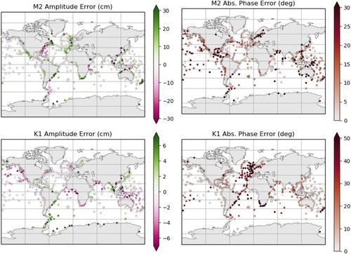
Figure 2. Amplitude and phase errors in the unadjusted model for M2 and K1 at available tide gauge and bottom pressure recorder locations.

2.4. Assimilation scheme

2.4.1. Overview

Data assimilation techniques are used to blend together SSH harmonics from the model and observed harmonics (discussed further in Section 2.4.2). Henceforth, the dataset of combined observations and model harmonics will be referred to as the ‘analysis dataset’, which is distinct from the harmonic analysis discussed in Section 2.5. Amplitudes and phases are not directly used in this scheme due to the periodicity of phase and strictly positive nature of amplitude. These characteristics create difficulties when applying modifications to the model (e.g. adjusted amplitudes must never be negative) and in ensuring that errors are normally distributed: a necessity for many assimilation schemes. Instead, $z_1$ and $z_2$ are used, defined here as: (1) $z_1=a\cos g,$(1) (2) $z_2=a\sin g,$(2) where a and g are the amplitude and phase, respectively, of a given constituent. These are the cartesian (or complex) analogue of amplitude and phase, and both lie in the set of real numbers, $\mathbb{R}$. This also aligns well with comments made by Xu (2018) on the interpolation of harmonic information. It is important to note that only the assimilation of SSH is discussed in this study. Options for extending this to currents are discussed in Section 4.

2.4.2. Ensemble optimal interpolation

To create the analysis dataset, with observations assimilated into the model simulation dataset (hereafter the ‘analysis’), Ensemble Optimal Interpolation (EnOI) is used (Oke et al., 2002; Evensen, 2003). As the name suggests, this is an ensemble version of Optimal Interpolation (Lorenc, 1986; Daley, 1991), where the analysis ${\mathbf{x}}_{\mathbf{a}}$ is obtained by solving the linear system: (3) ${\mathbf{x}}_a={\mathbf{x}}_b+\mathbf{K}(\mathbf{y}-{\mathbf{H}\mathbf{x}}_b),$(3) where ${\mathbf{x}}_b$ is the background variable, $\mathbf{y}$ is a vector of observations, $\mathbf{K}$ is the gain matrix and $\mathbf{H}$ is a linear operator which transforms variables in the background space to the observation space (often just interpolation). For this study, ${\mathbf{x}}_{\mathbf{b}}$ is harmonic analysis output for modelled SSH, linearly adjusted such that errors have no offset or trend (henceforth ‘linearly adjusted model’). The $\mathbf{y}$ is a vector of tide gauge and bottom pressure analyses as detailed in Section 2.3. The term $\mathbf{y}-{\mathbf{H}\mathbf{x}}_b$ is the innovation; a measure of the difference between the model and the observations. The $\mathbf{K}$ matrix describes a set of weights designed to minimise the error variance in the analysis and is determined using: (4) $\mathbf{K}=\mathbf{B}{\mathbf{H}}^T(\mathbf{H}\mathbf{B}{\mathbf{H}}^T+\mathbf{R}{)}^{-1},$(4) where $\mathbf{B}$ is the background error covariance matrix and $\mathbf{R}$ is the observation error covariance matrix. For this study, the background error covariance matrix $\mathbf{B}$ is estimated as the Schur product of a correlation function ρ and a covariance matrix ${\mathbf{B}}^{\mathrm{\prime }}$ (Houtekamer and Mitchell, 2001): (5) $\mathbf{B}=\rho \odot {\mathbf{B}}^{\mathrm{\prime }},$(5) where ${\mathbf{B}}^{\mathrm{\prime }}$ is the covariance matrix obtained from the ensemble of model-like variables ${\mathbf{x}}_i^{\mathrm{\prime }}$: (6) ${\mathbf{A}}^{\mathrm{\prime }}=\{{\mathbf{x}}_1^{\mathrm{\prime }},\dots ,{\mathbf{x}}_N^{\mathrm{\prime }}\}.$(6) The variables ${\mathbf{x}}_i^{\mathrm{\prime }}$ are model anomalies obtained by subtracting the ensemble mean from an ensemble, $\mathbf{A}$, of model states ${\mathbf{x}}_i$: (7) ${\mathbf{x}}_i^{\mathrm{\prime }}={\mathbf{x}}_i-\overline{\mathbf{A}},$(7) where, (8) $\mathbf{A}=\{{\mathbf{x}}_1,\dots ,{\mathbf{x}}_N\}$(8) For this study, the correlation function ρ is intended to ‘localize’ the assimilation increment, i.e. limit the spatial extent of an observations influence. If ρ is chosen correctly then the product in Equation (5(5) $\mathbf{B}=\rho \odot {\mathbf{B}}^{\mathrm{\prime }},$(5) ) retains the required properties of a covariance matrix. Gaspari and Cohn (1999) suggested a number of functions suitable for this purpose. We have chosen a simple single-variable Gaussian type function: (9) $\rho (r)=e^{-\frac{r^2}{\sigma }},$(9) where r is a great arc distance between two points and σ is a constant to be chosen. The function is isotropic and decreases with distance with a rate dictated by σ, which is defined globally and tuned independently for each constituent by minimising mean absolute errors in $z_1$ and $z_2$. This means that the localisation is homogeneous, which may not completely represent different length scales in the open ocean and coastal regions. However, it does preserve the required symmetry and positive semidefinite property of the covariance matrix (Gaspari and Cohn, 1999).

EnOI is closely related to the popular Ensemble Kalman Filter (EnKF) method (Evensen, 1994; Burgers et al., 1998), which has been used extensively in oceanic and atmospheric applications. It uses a covariance matrix which is stationary in time, applying a derived increment to a single deterministic model state. On the other hand, EnKF updates the covariance model by updating each member of the covariance ensemble at each application. As a result, EnKF is approximately N times more computationally expensive than EnOI. For our purposes, EnOI is sufficient, seeing as assimilation is done only into a single harmonic state, negating the need for an updated error covariance matrix (Oke et al., 2010).

2.4.3. Implementation

The ensemble used is comprised of 18 members, each being a harmonic analysis of a different model run. Bottom friction and β (used to model self-attraction and loading, see Section 2.2) are varied in each member in order to generate an appropriate spread in the resulting ensemble. More specifically, bottom friction is varied linearly 5% either side of the central value and β between 0.085 and 0.103. These two variables are highly influential in the generation and propagation of global tides in a barotropic model, and therefore the correct choice of value represents a significant portion of the error. For this study, the ensemble used is not expected to be optimal and there will be able to be improved. We discuss this further in Section 4.

In many ensemble assimilation methods (e.g. EnKF), the result is an ensemble of analyses. However, in this study, the ensemble is used only to generate an estimate of the background error covariance matrix $\mathbf{B}$. Each member of the ensemble is generated from a model run of 3 months. Observations are assimilated into a single ‘central’ background state, which is generated from a longer harmonic analysis of 1-year. The values used for bottom friction and β in this model run are those that lie in the centre of the ensemble values. This methodology allows us to estimate the background error covariance matrix with less expense than performing the full-length run for each ensemble member. It also allows us to perform the assimilation step just once.

For assimilation purposes, errors in $z_1$ and $z_2$ are assumed to be independent of each other (zero correlation). Though a strong assumption, preliminary tests showed it gave better results than allowing for cross-variable correlation. Assimilation is then done independently for each harmonic constituent.

The linear problem detailed in Equation (4(4) $\mathbf{K}=\mathbf{B}{\mathbf{H}}^T(\mathbf{H}\mathbf{B}{\mathbf{H}}^T+\mathbf{R}{)}^{-1},$(4) ) becomes very large for a global domain. A parallel routine was developed to overcome this problem. The routine works by splitting the global domain into smaller subdomains and an analysis is created independently for each. All available innovations from the global domain are used for each subdomain to ensure solutions are the same as the full problem. The background covariance matrix $\mathbf{B}$ is never constructed explicitly. Instead, only ${\mathbf{B}\mathbf{H}}^T$ and ${\mathbf{H}\mathbf{B}\mathbf{H}}^T$, as required for $\mathbf{K}$ (Equation (4(4) $\mathbf{K}=\mathbf{B}{\mathbf{H}}^T(\mathbf{H}\mathbf{B}{\mathbf{H}}^T+\mathbf{R}{)}^{-1},$(4) )), are calculated, consuming less memory.

2.5. Harmonic analysis

For both validation and the assimilation procedure, it is imperative that the harmonics from the model and observations are comparable. When using an assimilation scheme, the background and observed variables must represent the same quantity as best as possible. Therefore, a number of decisions and assumptions have been made in choosing a model harmonic analysis and selecting data for assimilation.

Model harmonics are obtained from a harmonic analysis of hourly sea surface height data. The diaharm module, packaged with NEMO, is used for this purpose. One year of model data is analysed for the final dataset, enough to resolve most major constituents, included those with longer periods. All forcing constituents are included in the analysis along with five nonlinear constituents. The choices of harmonic analyses of observed SSH varies per dataset and, in the case of bottom pressure recorders especially, per location. Observations to be included in the analysis are chosen based primarily upon the analysis length and available constituents. Specifically, only locations where K2 can be resolved (approximately six months or more (Foreman, 1996)) are chosen.

The period of time used for harmonic analysis of model data is different from that used for the observed data (which also varies from location to location). Therefore, by using this type of data, an assumption is made that the tidal harmonics are not changing significantly over the timescale of 20–30 years. It is likely that the tides are changing due to climate change (Pickering et al., 2017) ; however, these changes are likely to be small enough such that this assumption is not important in this context.

3. Results

3.1. Validation of raw model

Before examining the analysis dataset, we take a look at raw model output (no assimilation or adjustment) to understand how well it performs. In this section, we perform a validation of the central background state described in Section 2.4.3. We focus on three diurnal and three semi-diurnal constituents. Q1, O1, K1 and M2, S2 and K2. All available observations are used to evaluate the raw model – more than used in the actual assimilation or to validate the analysis in Section 3.2.

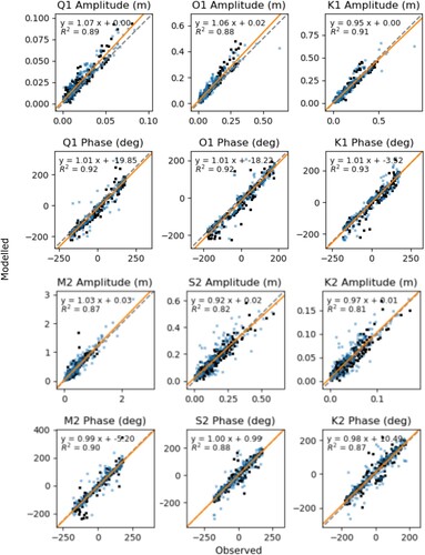
Figure 1 shows the observed amplitudes and phases plotted directly against the modelled amplitudes and phases at then nearest model grid point. The results of a linear regression are also shown, along with the $R^2$ of the fit. Ocean and shelf points have been defined as a location where the bathymetric depth is deeper/shallower than 200 m, respectively. These points are shown by different markers in the figures. For all constituents, the gradient of the data is good for both phase and amplitude. The largest deviations of gradients from unity are seen for Q1 and O1 amplitudes, reaching 1.07 and 1.06, respectively. Offsets are also generally small, especially for amplitudes. $R^2$ values are generally good, exceeding 0.85 in most cases ; however, there is some significant spread in some of the constituents. In many cases, larger outliers are seen in – but not limited to – points on the shelf. Larger errors in shallower/coastal regions are to be expected due to the relatively low resolution of the model and restrictions on depth (see Section 2.2). Overall, however, the model performs well, even in the absence of assimilation.

Figure 1. Scatter plots and lines of best fit for unadjusted modelled amplitude and phase against observed amplitude and phase for six of the larger diurnal and semi-diurnal constituents. Model points are extracted using a nearest neighbour approach. Orange line shows the best linear fit, black dots show ocean points ($>200\mathrm{m}$ depth) and blue squares show shelf points ($<200\mathrm{m}$ depth). The dashed grey line denotes y=x.

These errors can also be studied spatially. Figure 2 shows amplitude and phase errors on a geographic plot at observations locations. Spatial patterns in these errors vary considerably between the two constituents. In general, the magnitudes of amplitude errors are larger in regions where the amplitude is also larger, which is not surprising (see Figures 5 and 6 for amplitude magnitudes). Many of these areas are also coastal and/or have complex coastal geometry. For example the Bay of Fundy (northeast coastline of the North America) and some areas of the Northwest European Continental Shelf. Strong regional patterns are present in some areas. For instance, M2 amplitude is generally overestimated in the eastern Atlantic but underestimated in the Western Atlantic. The inverse of this is true in some regions for K1 amplitude, e.g. the eastern Atlantic and west coast of both Americas are underestimated. An area which stands out as having particularly large errors and also less of a consistent spatial pattern is the Western Pacific. Here, many areas are shallow and the complex island/coastal geometries are likely not well resolved.

Figure 5. A visual comparison of M2 in the dataset discussed in this paper (called GTM here) and FES2014.

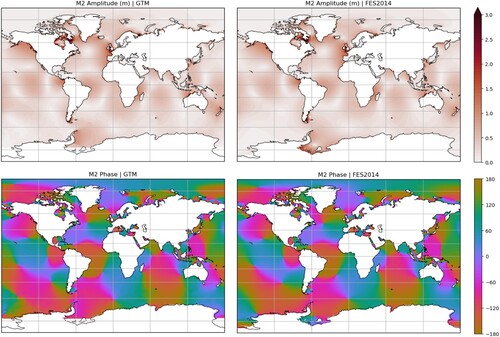
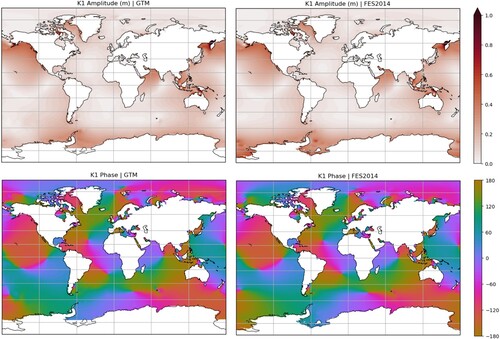
Figure 6. A visual comparison of K1 in the dataset discussed in this paper (called GTM here) and FES2014.

Consistent spatial patterns are also seen in phase. At most locations, errors in M2 phase are below ${30}^{\circ }$. Larger errors are typically seen along coastlines or in more enclosed areas such as the Baltic Sea and Gulf of Mexico. Again, a different pattern of errors is seen for K1 phase, with the largest errors being clustered in regions such as the eastern North Atlantic and western South Atlantic. In some regions, phase can be very sensitive to the exact location of an amphidromic point (point of zero amplitude), where small changes can result in large phase alterations.

3.2. Validation of analysis scheme

Validation can only be done at observation locations. However, The analysis dataset cannot be directly compared to observations as they have been incorporated into the data, giving high accuracy at observation locations. Instead of using the final analysis dataset, we take an ensemble approach to validation. For each constituent, a 120 member ensemble is created where in each member an analysis is generated as before but one third of observations, randomly chosen, are not included in the assimilation procedure. This means that in each ensemble member, we have a set of observations that can be used for validation. For this approach, observations are first thinned such that the minimum distance between any two points is 300 km. This is to reduce the effect of areas of relatively dense observations skewing the analysis.

Using the above ensemble, a new dataset is constructed by taking an ensemble at each observation location, but only when data was not included in the ensemble member. Henceforth, this dataset will be referred to as the ‘validation analysis’. Figures 3 and 4 show results from this process, which are discussed further below. Error statistics for the validation analysis are compared to those from model data that has not seen data assimilation. For this comparison, the linearly adjusted model output, as described in Section 2.4 and Table 1 is used. Tables 2 and 3 summarise the results.

Figure 3. Mean absolute errors (MAE) for six harmonic constituents in the linearly adjusted model output (marker locations) and validation analysis dataset (arrow tips). The arrow shows the change in MAE when comparing the two datasets. For each constituent, two arrows are shown. Those with circles around their marker corresponds to MAEs across shelf locations (depth $<200\mathrm{m}$) and those without correspond to ocean locations (depth $>200\mathrm{m}$).

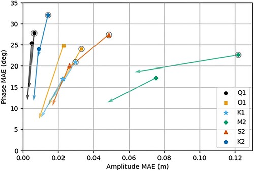
Figure 4. Correlation coefficients ($R^2$) for six harmonic constituents in the linearly adjusted model output (marker locations) and validation analysis dataset (arrow tips). The arrow shows the change in $R^2$ when comparing the two datasets. For each constituent, two arrows are shown. Those with circles around their marker corresponds to $R^2$ across shelf locations (depth $<200\mathrm{m}$) and those without correspond to ocean locations (depth $>200\mathrm{m}$).

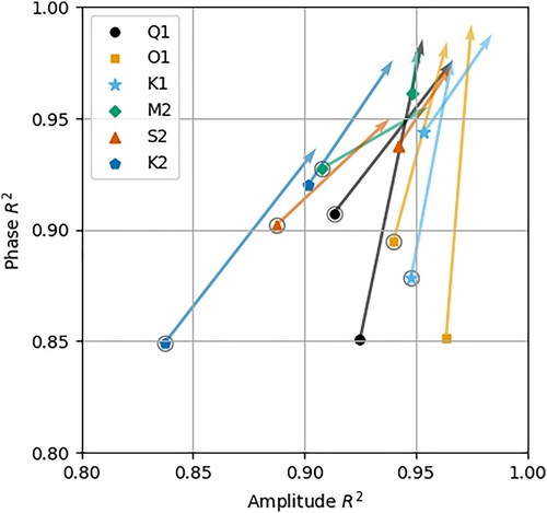
Table 2. Summary of amplitude MAE and correlation coefficients for the linearly adjusted model (LAM) and the validation analysis (VA).

$Amplitude(cm)$	MAE				$R^2$
Ocean	LAM	VA	Improvement	Points Improved	LAM	VA
Q1	0.49	0.26	47$\text{\%}$	71 $\text{\%}$	0.93	0.95
O1	2.28	0.96	58$\text{\%}$	75 $\text{\%}$	0.97	0.97
K1	2.36	1.10	53$\text{\%}$	80 $\text{\%}$	0.96	0.98
M2	7.50	4.64	38$\text{\%}$	73 $\text{\%}$	0.94	0.94
S2	2.63	1.63	38$\text{\%}$	72 $\text{\%}$	0.93	0.96
K2	0.85	0.58	31$\text{\%}$	74 $\text{\%}$	0.87	0.94
$Amplitude(cm)$	MAE				$R^2$
Shelf	LAM	VA	Improvement	Points Improved	LAM	VA
Q1	0.64	0.36	44$\text{\%}$	71 $\text{\%}$	0.91	0.97
O1	3.38	1.40	58$\text{\%}$	74 $\text{\%}$	0.94	0.97
K1	2.85	1.67	42$\text{\%}$	68 $\text{\%}$	0.94	0.96
M2	12.59	6.65	47$\text{\%}$	73 $\text{\%}$	0.91	0.96
S2	5.02	2.60	48$\text{\%}$	78 $\text{\%}$	0.91	0.94
K2	1.51	0.88	42$\text{\%}$	76 $\text{\%}$	0.86	0.91

‘Ocean’ locations refer to points where the bathymetric depth is deeper than 200 m and ‘Shelf’ locations to points shallower than this depth. Also shown is the percentage improvement in MAE and the percentage of points that were improved (in the validation analysis) by the scheme.

Table 3. Summary of phase MAE and correlation coefficients for the linearly adjusted model (LAM) and the validation analysis (VA).

$Phase(deg)$	MAE				$R^2$
Ocean	LAM	VA	Improvement	Points Improved	LAM	VA
Q1	26	12	52$\text{\%}$	82$\text{\%}$	0.84	0.97
O1	25	7	71$\text{\%}$	89$\text{\%}$	0.84	0.98
K1	17	8	55$\text{\%}$	74$\text{\%}$	0.94	0.98
M2	16	10	34$\text{\%}$	71$\text{\%}$	0.96	0.96
S2	20	10	52$\text{\%}$	75$\text{\%}$	0.93	0.97
K2	25	11	54$\text{\%}$	79$\text{\%}$	0.91	0.98
$Phase(deg)$	MAE				$R^2$
Shelf	LAM	VA	Improvement	Points Improved	LAM	VA
Q1	27	14	48$\text{\%}$	77 $\text{\%}$	0.92	0.95
O1	23	11	55$\text{\%}$	83 $\text{\%}$	0.89	0.97
K1	19	12	39$\text{\%}$	72 $\text{\%}$	0.88	0.97
M2	24	19	20$\text{\%}$	71 $\text{\%}$	0.92	0.94
S2	27	19	28$\text{\%}$	70 $\text{\%}$	0.91	0.93
K2	32	21	31$\text{\%}$	73 $\text{\%}$	0.86	0.89

‘Ocean’ locations refer to points where the bathymetric depth is deeper than 200m and ‘Shelf’ locations to points shallower than this depth. Also shown is the percentage improvement in MAE and the percentage of points that were improved (in the validation analysis) by the scheme.

Figure 3 shows a comparison of Mean Absolute Errors (MAE) in amplitude and phase of the linearly adjusted model and validation analysis. Amplitude MAE and phase MAE are plotted on different axes, meaning that a movement towards the origin indicates an average improvement in the validation analysis when compared to the linearly adjusted model. Values have been calculated separately for observations on the shelf (depths shallower than 200 m) and in the open ocean (depth exceeding 200 m). In almost all cases, amplitude and phase MAE are larger in the shallower areas for both the linearly adjusted model and validation analysis. The exception is O1, for which the shelf phase error is slightly smaller than that in the open ocean. In all cases, MAEs are at least 30$\text{\%}$ lower for the validation analysis than the linearly adjusted model suggesting that, on average, errors are indeed being reduced. As can be seen in Tables 2 and 3, this reduction is as much as $58\text{\%}$ for amplitude and $71\text{\%}$ for phase (both for O1).

Figure 4 shows how well the linear adjusted model and validation analysis correlate with observations using the Spearman's Rank correlation coefficient $R^2$. Similarly to Figure 3, amplitude and phase values are plotted on separate axes. In this case, a movement towards $(1,1)$ shows where the validation analysis had a higher correlation coefficient than the linearly adjusted model. Mirroring the MAE case, Correlations are generally lower in shelf regions but still high in most cases. For every constituent, the validation analysis improves correlations for both amplitude and phase. For some constituents, this improvement is modest, for example, M2. Others see significant improvement such as Q1 and O1 phase.

Improvements in MAE and correlations at locations not included in the analysis show that, on the whole, the analysis scheme is spreading innovations into the domain realistically. The scheme is not perfect, however, which is demonstrated by the number of points which do not see improvement and MAE/correlations have room for further improvement. However, these results give confidence in the analysis schemes ability to blend observed data into the modelled harmonics. This is especially true for the final analysis, which incorporates many more observations.

3.3. Analysis dataset

In this section, we visually compare the analysis datasets generated for this study to another prominent tidal dataset: FES2014 (Carrere et al., 2016). This comparison allows for an inspection of large scale regions where the datasets vary and to reason why. These comparisons are shown in Figures 5 and 6 for M2 and K1, respectively. Other constituents are not discussed here ; however, the conclusions remain the same. For this section we refer to our dataset as GTM (Global Tide Model). It is important to note that in this section we do not intend to make a direct comparison with FES2014 or to improve upon it ; however, we choose to use this dataset as a broad check that our scheme works over large scales.

Figure 5 shows amplitude and phase comparisons for M2. The datasets compare well for both variables, especially away from the poles. The locations of many major amphidromes (identified as areas of strong phase gradient and zero amplitude) are similar in many regions, for example in the North Atlantic, Northeast Pacific and Northwest Pacific. Even in some shallower more coastally complex regions, such as the North Sea and Caribbean Sea, these systems compare well. There are also areas of notable difference. An amphidrome in the FES2014 Weddell sea is missing (or perhaps degenerate) in the GTM dataset. This is likely due to differences in domain extent, as the domain used for GTM does not extend as far south as the FES2014 domain. Another notable area of difference is the Southeast Pacific. This is an area where tide gauge and bottom pressure observations are sparse (see Figure 2).

Figure 6 shows comparisons for K1. Again the two datasets compare well; however, the Southern Ocean shows some large differences in both amplitude and phase, especially in the South Pacific which, as already noted, is an area of limited tide gauge and bottom pressure observations. There are also some smaller scale amplitude features seen in the FES2014 Wedell and Ross Seas that are not present in the GTM dataset. This is again most likely due to domain constraints and the lack of ice modelling in our model. Overall, these results suggest that our method works well – where observations are available.

4. Discussion

In this study, the generation of a global dataset of tidal harmonics was described and evaluated. The method used data assimilation techniques to combine modelled and observed sea surface height harmonics. A full year of model data (from a NEMO configuration) was used to obtain harmonic information which was in turn combined with harmonic data from tide gauges and bottom pressure recorders. The assimilation procedure is completely offline, i.e. data assimilation is performed in a post-processing step rather than on a time step basis within the model. In addition, an ensemble is used only for covariance estimation, with each member being a truncated, shorter version of the full assimilative run. As a result, computation is relatively inexpensive compared to online assimilation or methods using an ensemble of full-length model runs, and the system is flexible, allowing for fast updates to the dataset whenever new simulated or observed data becomes available.

The assimilation scheme was validated using a specially constructed validation dataset, generated from an ensemble of analyses. In each member of this ensemble, one third of the observations were randomly omitted and it is at these locations that the validation was performed. This approach suggested that the assimilation scheme was able to reduce MAEs and increase correlation coefficients for both amplitude and phase in regions where observations were sparse. When averaged across all locations, improvements were seen in all constituents. However, improvements were not seen at all locations. Our validation analysis shows that in all cases, a percentage of points saw no significant improvement – approximately 20–30% for both amplitude and phase. There are numerous reasons why this may be the case, which we discuss in the following paragraphs.

The assimilation of $z_1=a\sin g$ and $z_2=a\cos g$ means that only harmonic data may be used and there are fundamental limitations associated with the offline assimilation of harmonics, limiting the available observations to locations where time series are sufficiently long. Increments are also constrained to regions near observations. The lack of forward model in the assimilation procedure means that increments will not propagate dynamically from areas with observations to those without, as would be the case for online assimilation of sea surface height. Although spatial propagation of information will be captured by the ensemble covariance method, regions which have sparse observations may see little improvement or gain a noisy characteristic, as seen in Section 3.3 for the South Pacific. This may partially explain why some regions do not see any significant improvement.

Changes to the numerical model could result in better background data and a more representative ensemble used to generate the background error covariance. For example, higher resolution in coastal areas, a relaxed restriction on bathymetric depth and the inclusion of ice into the model. Physical parameterisations could be further tuned, improved or even replaced. For example, in this study the scalar approximation method was used to parameterise self-attraction and loading; however, other methods with better accuracy are available (Ray, 1998; Stepanov and Hughes, 2004) such as iterative methods (Accad and Pekeris, 1978) and Green's Function methods (Hendershott, 1972; Farrell, 1973). These methods can be computationally costly, however, and were beyond the scope of this work. The dissipation of barotropic tidal energy in the open ocean is also very important for global tide modelling (Jayne and Laurent, 2001; Simmons et al., 2004). The parametrisation used for this work is a simple scale relation and could be improved. Full modelling of internal physics could also be done if vertical density profiles were not homogeneous (and a higher resolution model was used).

The ensemble used for estimation of the background covariance matrix in this paper is not optimal and could be improved. Future work is required to iterate upon it and improve its representation of the model error, leading to innovations being spread from the observation point into the domain in a more realistic fashion. The ensemble used in this paper is not optimal and This may mean improving the physical model or the statistical decisions made when designing the ensemble itself. The ensemble used for this study was small (18 members) and limited. Despite this, however, our scheme worked well and improved the model at the majority of locations.

The construction of the covariance matrix itself may also benefit from further iteration. In this paper, it is constructed from the combination of the ensemble covariance and a Gaussian localisation function. Although this worked for our purposes, this could be improved. For example, the localisation function uses haversine distance as a parameter, which may not be the best choice in the presence of complex coastlines and islands. Signals propagate around coastal boundaries, not through them as implied by such a distance metric. For future work, other methods are available, such as shortest-path methods (see Byrne et al. (2021)), which calculate distances around coastal boundaries, although these methods may be costly on a global domain. The Gaussian function used also assumed spatial homogeneity and isotropy. Although these assumptions simplify the analysis procedure, investigations into using different lengths scales in different regions (e.g. open ocean and on the shelf) may improve the methodology further.

An important limitation to note is that of the variance in harmonic analyses used for both the observations and model. It was mentioned in Section 2.5 that the observed and modelled tidal harmonics were all derived from different time periods of data. In addition to this, however, these were also calculated using different analysis parameters: analysis length, analysis period, constituent sets and software choice. This may result in some representativity error when comparing model harmonics with the observations, which will subsequently find its way into the analysis dataset. The alternative is a vastly reduced observation dataset due to the lack of original time series and the need to run the model for a limited period. For this study, we accept this uncertainty but it will require further study in the future.

Finally, creating dynamically consistent barotropic currents can be a challenge, although options are available. SSH harmonics can be inverted using a method such as that outlined by Ray (2001). Such a method, however, means having to solve very large systems of equations on a global domain. Alternatively, SSH-current covariances can be determined from an ensemble and used to adjust currents within a multivariable assimilation scheme such as those by Lorenc (1981), Courtier et al. (1998), and Lorenc et al. (2000).

The limitations of the simulation physics provide a greater challenge for the offline assimilation scheme that is presented here. Nevertheless the scheme is demonstrated to improve Mean Absolute Errors and correlation coefficients across the largest diurnal and semi-diurnal constituents.

Acknowledgements

We would like to thank the NERC National Capability programme: Climate Link Atlantic Sector Science (CLASS).

Disclosure statement

No potential conflict of interest was reported by the author(s).

Data availability statement

The numerical model was run on the ARCHER computing cluster and output data was processed using the Python language, including the numpy, scipy and matplotlib libraries. The source code for the model, including modifications for this work, can be found at https://github.com/NOC-MSM/global_tide. This link also includes the tidal forcing values used. Other input datasets are all cited within this manuscript, include ERA5 atmospheric data (https://www.ecmwf.int/en/forecasts/datasets/reanalysis-datasets/era5) and GEBCO bathymetric data (https://www.gebco.net/data_and_products/gridded_bathymetry_data/).

References

- Accad Y, Pekeris CL. 1978. Solution of the tidal equations for the M2 and S2 tides in the world oceans from a knowledge of the tidal potential alone. Phil Trans R Soc Lond. 290(1368):235–266.
- Arbic BK, Wallcraft AJ, Metzger EJ. 2010. Concurrent simulation of the eddying general circulation and tides in a global ocean model. Ocean Model. 32:175–187.
- Burgers G, van Leeuwen PJ, Evensen G. 1998. Analysis scheme in the ensemble Kalman filter. Monthly Weather Rev. 126:1719–1724.
- Byrne D, Horsburgh K, WIlliams J. 2021. Variational data assimilation of sea surface height into a regional storm surge model: Benefits and limitations. J Oper Oceanogr. DOI:10.1080/1755876X.2021.1884405.
- Carrere L, Lyard F, Cancet M, Guillot A, Picot N. 2016. Fes 2014, a new tidal model – validation results and perspectives for improvements. presentation to ESA Living Planet Conference, Prague.
- Cartwright DE, Taylor RJ. 1971. New computations of the tide-generating potential. Geophys J R Astr Soc. 23:45–74.
- Cartwright DE, Zetler BD, Hamon BV. 1979. Pelagic tidal constants. IAPSO Public Sc. 33.
- Courtier P, Andersson E, Heckley W, Pailleux J, Vasiljevic D, Hamrud M, Hollingsworth A, Rabier F, Fisher M. 1998. The ECMWF implementation of three-dimensional variational assimilation (3D-var). i: Formulation. Q J R Meteorol Soc. 124:1783–1807.
- Daley R. 1991. Cambridge Atmospheric and Space Science Series. Cambridge: Cambridge University Press. ISBN 0521 382157. https://doi.org/10.1002/joc.3370120708.
- Egbert GD, Bennett AF. 1996. Data assimilation methods for ocean tides. In: Modern approaches to data assimilation in ocean modelling. Elsevier Oceanography Series, Elsevier.
- Egbert GD, Erofeeva SY. 2002. Efficient inverse modelling of barotropic ocean tides. J Atmospheric Oceanic Technol. 19:183–204.
- Egbert GD, Ray RD. 2000. Significant dissipation of tidal energy in the deep ocean inferred from satellite altimeter data. Nature. 405:775–778.
- Evensen G. 1994. Sequential data assimilation with a nonlinear quasi-geostrophic model using monte carlo methods to forecast error statistics. J Geophys Res. 99:10143–10162.
- Evensen G. 2003. The ensemble Kalman filter: theoretical formulation and practical implementation. Ocean Dyn. 53:343–67.
- Farrell WE. 1973. Earth tides, ocean tides and tidal loading. Phil Trans R Soc Lond. 274:253–259.
- Foreman MGG. 1996. Manual for tidal heights analysis and prediction. 5th ed. Institute of Ocean Sciences, Patricia Bay, Sydney.
- Foreman MGG, Neufeld ET. 1991. Harmonic tidal analyses of long time series. Int Hydrographic Rev. 68:85–108.
- Gaspari G, Cohn SE. 1999. Construction of correlation functions in two and three dimensions. Q J R Meteorol Soc. 125(554):723–757.
- GEBCO Compilation Group. 2020. GEBCO 2020 Grid. doi:10.5285/a29c5465-b138-234d-e053-6c86abc040b9.
- Hendershott MC. 1972. The effects of solid earth deformation on global ocean tides. Geophys J R Astr Soc. 29:389–402.
- Holgate SJ, Matthews A, Woodworth PL, Rickards LJ, Tamisiea ME, Bradshaw E, Foden PR, Gordon KM, Jevrejeva S, Pugh J. 2013. New data systems and products at the permanent service for mean sea level. J Coastal Res. 29(3):493–504.
- Houtekamer PL, Mitchell HL. 2001. A sequential ensemble Kalman filter for atmospheric data assimilation. Monthly Weather Rev. 129:123–137.
- Jayne SR, Laurent LCS. 2001. Parameterizing tidal dissipation over rough topography. Geophys Res Lett. 28(5):811–814.
- Large WG, Yeager S. 2004. Diurnal to decadal global forcing for ocean and sea-ice models: the data sets and flux climatologies. Technical report, NCAR technical note, NCAR/TN-460+STR, CGD Division of the National Center for Atmospheric Research.
- Lorenc AC. 1981. A global three-dimensional multivariate statistical interpolation scheme. Monthly Weather Rev. 109:701–721.
- Lorenc AC. 1986. Analysis methods for numerical weather prediction. Q J R Meteorol Soc. 112:1177–1194.
- Lorenc AC, Ballard SP, Bell RS, Ingleby NB, Andrews PLF, Barker DM, Bray JR, Clayton AM, Dalby T, Li D, Payne TJ, Saunders FW. 2000. The met office global three-dimensional variational data assimilation scheme. Q J R Meteorol Soc. 126(570):2991–3012.
- Madec G. 2008. NEMO Ocean Engine. Note from the School of Modeling, Pierre-Simon Laplace Institute (IPSL), France, No. 27, ISSN No. 1288–1619.
- Madec G, Imbard M. 1996. A global ocean mesh to overcome the north pole singularity. Clim Dyn. 12:381–388.
- Oke PR, Allen JS, Miller RN, Egbert GD, Kosro PM. 2002. Assimilation of surface velocity data into a primitive equation coastal ocean model. J Geophys Res. 107(C9):3122.
- Oke PR, Brassington GB, Griffin DA, Schiller A. 2010. Ocean data assimilation: a case for ensemble optimal interpolation. Australian Meteorol Oceanographic J. 59:67–76.
- Parke ME, Hendershott MC. 1980. M2, s2, k1 models of the global ocean tide on an elastic earth. Marine Geodesy. 3:379–408.
- Pekeris CL, Accad Y. 1969. Solution of Laplace's equations for the m2 tide in the world oceans. Phil Trans R Soc. 265(1165):413–436.
- Permanent Service for Mean Sea Level. 2019, Jun. Tide gauge and bottom pressure data. Technical Report, http://www.psmsl.org/data/obtaining/.
- Pickering MD, Horsburgh KJ, Blundell JR, Hirschi JJM, Nicholls RJ, Verlaan M, Wells NC. 2017. The impact of future sea-level rise on the global tides. Cont Shelf Res. 142:50–68.
- Pugh D, Woodworth P. 2014. Sea level science: Understanding tides, surges, tsunamis and mean sea-level changes. Cambridge University Press. doi:10.1017/CBO9781139235778.
- Ray RD. 1998. Ocean self attraction and loading in numerical tidal models. Marine Geodesy. 21:181–192.
- Ray RD. 1999. A global ocean tide model from Topex/Poseidon altimetry: Got99.2. NASA Tech. Memo. 209478, Goddard Space Flight Center, Greenbelt, MD, p. 58.
- Ray RD. 2001. Inversion of oceanic tidal currents from measured elevations. J Mar Syst. 28:1–18.
- Schwiderski EW. 1979. Global ocean tides: Part II. The semidiurnal principal linear tide 884 (m2), atlas of tidal charts and maps. Technical report, Naval Surface Weapons Center, Dahlgren, VA.
- Simmons HL, Jayne SR, Laurent LCS, Weaver AJ. 2004. Tidally driven mixing in a numerical model of the ocean general circulation. Ocean Model. 6:245–263.
- Stammer D, Ray RD, Andersen OB, Arbic BK, Bosch W, Carrère L, Cheng Y, Chinn DS, Dushaw BD, Egbert GD, Erofeeva SY, Fok HS, Green JAM, Griffiths S, King MA, Lapin V, Lemoine FG, Luthcke SB, Lyard F, Morison J, Müller M, Padman L, Richman JG, Shriver JF, Shum CK, Taguchi E, Yi Y. 2014. Accuracy assessment of global barotropic ocean tide models. Rev Geophys. 52:243–282.
- Stepanov VN, Hughes CW. 2004. Parametrization of ocean self-attraction and loading in numerical models of the ocean circulation. J Geophys Res. 109. doi:10.1029/2003JC002034.
- Storkey D, Blaker AT, Mathiot P, Megann A, Aksenov Y, Blockley EW, Calvert D, Graham T, Hewitt GT, Hyder P, Kuhlbrodt T, Rae JGL, Sunha B. 2018. UK global ocean go6 and go7: a traceable hierarchy of model resolutions. Geoscientific Model Development. 11:3187–3213.
- Taguchi EW, Zahel W, Stammer D. 2014. Inferring deep ocean tidal energy dissipation from the global high-resolution data-assimilative Hamtide model. J Geophys Res – Oceans. 119:4573–4592.
- Woodworth PL, Hunter JR, Marcos M, Caldwell P, Menéndez M, Haigh I. 2017. Towards a global higher-frequency sea level dataset. Geosci Data J. 3:50–59.
- Xu Z. 2018. A note on interpreting tidal harmonic constants. Ocean Dyn. 68:211–222.