Comparative evaluation of CO₂ concentrations across administrative regions with temperate climates in Northeast Asia: potentials and constraints

ABSTRACT

This paper examined carbon concentrations across administrative regions with temperate climates in Northeast Asia (NEA) using Level 3 data of column-averaged CO₂ concentrations (XCO₂) that were derived from the Greenhouse Gases Observing Satellite (GOSAT) National Institute for Environmental Studies (NIES) retrieval algorithm. Data were analyzed for March through June 2009–2012 (boreal spring). The highest and lowest XCO₂ concentrations ranged from 397.7 to 384.1ppm, and the estimated XCO₂ distribution across administrative regions varied widely between 394.3 and 387.2 ppm. Low values were observed in the northern region of the study area (northern part of central China and South Korea). In contrast, high concentrations of XCO₂ were observed in the southeastern (Japan) and southwestern (China) regions. The five cities with the highest concentrations were located in China (Shanghai, Zhejiang and Jiangsu) and Japan (Kyushu and Shikoku). Among the 27 administrative regions analyzed, Kyushu showed the highest levels. There is still considerable debate about whether GOSAT data have sufficient reliability. This paper represents an early effort to compare carbon concentrations across administrative regions. Therefore, caution should be exercised when using the ranking numbers as a basis for regional comparisons.

Keywords:

• XCO₂
• administrative regions
• GOSAT
• Northeast Asia

Introduction

Political lines are usually drawn through regions with similar ecological and biological characteristics (hydrology, native vegetation structure, surrounding physical landscape, natural resources, agricultural conditions, etc.); thus, these regions are populated by culturally similar groups of people in terms of lifestyle features such as architectural structures and heating/cooling systems. Administrative boundaries strengthen the sense of belonging to a given region and they accommodate interdependent relationships through transportation, commerce and communication (e.g., postal and area codes). The existence and function of political boundaries can have considerable influence on the spatial development of industrial processes and the pattern of energy consumption, and, in particular, they are bisected by national jurisdictions and governance mechanism frontiers at the local level [1,2]. Urban areas are currently responsible for two thirds of the world's energy demand and carbon dioxide (CO₂) emissions, a share that is likely to grow with continued global urbanization [3]. In many countries, it is cities rather than the national government that have taken the lead role in reducing GHG emissions [4].

Establishing a goal to develop low-carbon cities requires good measurement tools for GHG accounting that depends on the availability of high-quality data, which implies transparency, consistency, completeness and accuracy [5]. Many administrative regions of the world have carried out carbon inventories, and recent literature compares the carbon footprint of large cities or metropolitan areas [6–8]. However, the comparability of reporting data between administrative regions is limited due to varying methodologies and frequency [9]. The United Nations Environment Programme (UNEP), the World Bank and UN-Habitat recently presented a standard for urban GHG emission reporting at the World Urban Forum [10]. The city network International Council for Local Environmental Initiatives (ICLEI) has presented its proposal for such a standard too [11]. If administrative regions would report carbon concentrations regularly and based on a common reporting format and city-specific data, carbon concentration data would be comparable and illustrate administrative region-specific carbon concentration trends. However, while voluntary frameworks have been suggested, no internationally accepted standard methodology currently exists providing detailed guidance for the collection of administrative region-based carbon concentration. Comparing administrative regions for their carbon emissions, activities and policies needs a very detailed and careful look. A comparative perspective provides important insights but is often challenging, especially in the case of administrative regions where information is scarce and unconsolidated [12]. The lack of a standardized method for city-scale GHG emissions accounting to date has produced inconsistent accounting approaches for cities throughout the world. However, carbon concentration data from different administrative regions are hardly comparable, because the frequency (time profiles), their long-term (and short-term) implications and methodologies used for carbon inventories vary significantly, and sometimes data quality may be poor [13]. There is a need to establish standardized GHG emission accounting protocols that provide consistent, reproducible, comparable and holistic GHG accounting [14].

Two observational approaches have traditionally been used to estimate carbon concentrations at the level of administrative regions. The top-down approach utilizes atmospheric CO₂ concentrations and transport models to retrieve biosphere fluxes across regional and continental scales [15,16]. Since no single model is a true representation of bio-geophysical processes, all model-based estimates of bio-geophysical variables are subject to large uncertainty. On the other hand, bottom-up, ground-based CO₂ observations are too sparse to sufficiently reduce uncertainty in the characterization of sources and sinks. Some of the major disadvantages of traditional field-monitoring techniques are that they are costly, laborious, and time-consuming because they require large sample sizes. Therefore, existing top-down or bottom-up carbon observations are not practical in terms of their cost or scientific reliability for area-wide approaches. Few studies have empirically examined spatial variations in CO₂ concentrations across administrative regions, despite growing interest in this issue [17,18].

Satellite data observing GHG may provide spatially and temporally consistent estimates of CO₂ concentrations to complement in situ observations and top-down methodologies. Developed by Japan, the Greenhouse Gases Observing Satellite (GOSAT), which was launched successfully on 23 January 2009, monitors total column CO₂ (denoted XCO₂) on the Earth's surface. GOSAT is the orbiting instrument that measures near-infrared (NIR) radiation with sufficient spectral resolution to retrieve values of XCO₂, and it has enabled extensive geographical coverage and frequent observations of XCO₂ density at high resolutions for regional or global analyses. Since its development, GOSAT has emerged as an important research topic in various fields. Many approaches have been proposed from different perspectives to ensure the reliability of GOSAT data. Therefore, it is recognized as one of the most powerful sensors currently available for CO₂ monitoring in terms of spatial as well as spectral resolution.

There is no universally accepted standard approach to using GOSAT data for comparative analyses of CO₂ concentrations across administrative regions in specific climate zones. Therefore, there is an urgent need to ensure consistency and conformity of GOSAT CO₂ mapping across administrative regions linked to climate zones. This paper presents the potentials and limitations of the use of GOSAT data to monitor XCO₂ concentrations across administrative regions with a temperate climate in Northeast Asia (NEA; China, South Korea and Japan). The overarching objective of this work is to determine how much information GOSAT observations can provide when comparing XCO₂ distributions at the level of administrative regions with a temperate climate.

Materials and methods

Study area and Level 2 data collection

The temperate NEA region generally refers to a large area consisting of China, southern Japan and the Republic of Korea (ROK) that stretches from 30 to 40°N latitude and from 115 to 135°E longitude (Figure 1). It has several advantages that make it an appropriate choice for this work. Recent economic and social development in NEA has come with the heavy cost of environmental degradation and the creation of highly energy-intensive industries and energy-dependent societies. The countries in NEA rank first among countries in Asia and the Pacific in terms of consumption pressure on environmental resources. In addition, the regional energy demand is expected to almost double by 2020. Currently, NEA countries account for 32% of global CO₂ emissions [19].

Figure 1. The study area and 222 points of National Institute for Environmental Studies Level 2 data (observations) for March to June 2009–2012.

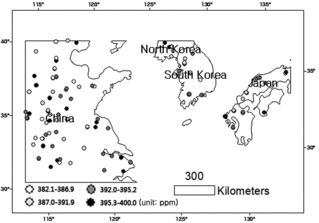
Meteorological conditions play an important role in CO₂ formation, transfer and dispersion. The NEA region has strong southeast summer winds and northwest winter winds. These seasonal winds are greatly influenced by the East Asian monsoon weather pattern. Carbon dioxide levels in summer or winter may vary widely because of unsteady sunshine and rainfall such as that typically seen during warm, rainy summer monsoons and cold, dry winter monsoons. As a result, Level 2 data points during these seasons were very scarce for the NEA region. In general, spring and fall are expected to show steady CO₂ levels because local meteorological conditions are relatively stable [20,21]. However, in autumn, the GOSAT observations have very poor coverage in the experimental area because of persistent cloudiness, as indicated by Hammerling et al. [22]. The terrestrial carbon cycle is strongly affected by natural phenomena, terrain heterogeneity and human activities that alter carbon exchange via vegetation and soil activities. In order to accurately understand terrestrial carbon cycle mechanisms, it is necessary to observe the growing season giving rise to high variability in XCO₂. Based on initial investigations of temporal resolutions ranging from 1 month to over a specific season, a resolution of 4 months was sufficient to obtain 232 Level 2 data points in the study area. GOSAT data products are processed at various levels ranging from Level 1 to Level 4. Level 1 products are raw data at full instrument resolution. The Level 1 data contain spectra and radiances acquired by the satellite. At higher levels, the data are converted into more useful formats accommodating parameters given by users. For instance, Level 2 data can store retrieved physical quantities such as the atmospheric concentrations of CO₂ and CH₄. Among these, only the Level 1 data and some of the Level 2 data products are validated, and their systematic errors are characterized in the vicinity of 12 stations of the Total Carbon Column Observing Network (TCCON).

Thus, this paper used GOSAT Level 2 data [the operational National Institute of Environmental Studies (NIES) short-wavelength infrared (SWIR) version 2.21 XCO₂ product (V01.xx; note that “xx” refers to different versions of the Level 1B product used in L2 processing)] for March to June (boreal spring) 2009–2012 (Figure 1) to identify the overall distribution of CO₂ concentrations.

The GOSAT is equipped with two instruments: the thermal and near infrared sensor for carbon observation–Fourier transform spectrometer (TANSO–FTS) and the cloud and aerosol imager (TANSOCAI). The TANSO–FTS obtains high spectral-resolution data in the SWIR (Bands 1, 2 and 3 centered at 0.76, 1.6 and 2.0 μm, respectively) and in the thermal infrared (TIR; Band 4 at 5.5–14.3 μm) regions of the electromagnetic spectrum. The Japan Aerospace Exploration Agency (JAXA) is responsible for producing calibrated radiances [released as a Level 1B (L1B) product], while NIES of Japan is responsible for the development of algorithms to retrieve the column-averaged dry-air mole fractions of CO₂ [XCO₂; released as a SWIR Level 2 (L2) product] from SWIR spectra and validating the retrieved XCO₂ from the SWIR L2 products [23].

The GOSAT samples the same location every 3 days and has a nadir footprint of 10.5 km in diameter (86.6 km² area). Global CO₂ distributions are created by inversion with a radiative transfer model, and sources and sinks of CO₂ are retrieved. Details about the retrieval method are provided by Yokota et al. [24]. Retrieved XCO₂ values are validated and their systematic errors are characterized in the vicinity of 12 stations of the TCCON. The TCCON is composed of ground-based Fourier transform spectrometers distributed throughout the world that provide measurements of XCO₂. The TCCON provides an essential validation resource for data from the GOSAT. A full description of the technology is beyond the scope of this paper (for further information, please visit the TCCON website [101]).

Inter-annual variability in CO₂ concentrations reflects land use and terrestrial biosphere responses caused by climate. Plant respiratory processes are sensitive to temperature and have generally been shown to increase with short-term warming [25,26]. Changes in rainfall patterns can influence the availability of plant water and the length of the growing season. To a large extent, the climate determines the type of soil and natural vegetation in a given region, and has considerable influence on land use. In particular, the climate dictates how buildings are designed and constructed and influences energy use in built environments. It is well known that spatial variations of terrestrial ecosystems, which are driven by changes in surface temperature and precipitation, are the dominant drivers of variability in atmospheric CO₂ [27]. Thus, warm years tend to be associated with higher plant growth rates and more inter-annual atmospheric CO₂ variability, whereas cool years tend to be associated with reduced growth rates and lower CO₂ variability.

Climate zone boundaries are drawn in relation to the vegetation distribution by combining average annual and monthly temperatures and precipitation. This approach to designating specific climate zones is expected to reduce data uncertainty associated with meteorological conditions and local biosphere fluxes, since spatial variability of XCO₂ such as retrieval errors would be restricted within the spring season of temperate regions. In this paper, the Köppen–Geiger classification method was used to extract the temperate climate zone. Although the climate classification concept introduced by Köppen–Geiger is still appropriate, the world classification has been recently updated by the use of large global data sets of long-term monthly precipitation and temperature time series [28,29]. Previous studies have provided detailed descriptions of the Köppen–Geiger criteria used for climate zone classifications [28]. Across countries in the study area, three out of the 30 possible climate classifications were identified (see Table 1).

Table 1. Temperate climate zone observed in the study area (Köppen-Geiger climate classifications).

Name	Main climate	Precipitation	Temperature
Cfa	Warm temperate	Fully humid	Hot summer
Cwa	Warm temperate	Humid	Hot summer
Cwb	Warm temperate	Humid	Warm summer

There may be differences in understanding of the definition and boundary of administrative regions among researchers, which can make CO₂ concentrations from cities difficult to compare. Administrative regions range from large nation-states to small administrative districts and suburbs. The world political boundary map developed by Environmental Systems Research Institute (ESRI) was used here to extract administrative boundaries at the first level (provinces and states). This map is updated twice a year. The mapping data set is composed of boundary files at national and provincial levels. Provincial-level data separate administrative regions into individual provinces and autonomous regions. The Zonal Statistics tool in ArcGIS Spatial Analyst software (version 10.0) was used to determine average carbon concentrations for each administrative boundary polygon from kriged (rasterized) data. Administrative boundaries were divided by climate zones to identify spatially intensified carbon concentrations. Data from administrative units are usually represented as a choropleth map. The display of carbon concentrations in the form of a chloropleth map first requires that the data be classified into a small number of class intervals, and then a graphic value is assigned to represent statistical values for all area units belonging to the same class interval. Carbon concentrations were aggregated into four class intervals by grouping them based on natural breaks [30], whereby the author considered the lowest and highest values to describe the spatial distribution pattern of concentration ranges in a more abstract form.

National Institute for Environmental Studies short-wavelength infrared Level 3 map generation

The GOSAT records often suffer from missing data values, mainly due to unfavorable meteorological conditions during the specific time periods of data acquisition. The FTS SWIR Level 3 data products are generated by interpolating, extrapolating and smoothing the FTS SWIR Level 2 column-averaged mixing ratios of CO₂. These data products can be utilized for visualizing local highs and lows of the greenhouse gases on a global scale. Because GOSAT data need to be estimated for areas beyond sampling sites, geostatistic interpolation can be used to estimate unsampled locations and produce surface maps [31,32]. Geostatistic interpolation obtains estimates of values for variables at unsampled locations by considering the spatial distribution patterns and integrating information from sample points and observed or known trends. The procedure is basically composed of the following three steps: exploration of statistical data, variogram analyses and the evaluation of results. The kriging approach draws information about the degree of spatial variability of XCO₂ directly from the XCO₂ observations without using additional information introduced from an atmospheric transport model or CO₂ flux estimates [32]. As such, the resulting Level 3 maps are a more direct representation of the information content of the available CO₂ retrievals, unlike maps derived from inverse modeling or data assimilation studies. Rather than being intended as inputs to inverse modeling studies, these Level 3 XCO₂ products enable direct independent comparisons with existing models of carbon flux and atmospheric transport [32].

It is known that normality is not a prerequisite for using kriging interpolators, but normality is a desirable property because interpolators generate only the best absolute predictions if the random function fits a normal distribution [33]. Extremely low-value outliers (356.65–382 ppm) are observed in GOSAT Level 2 data. In the kriging interpolation, such data may have a significant impact on interpolation results, and therefore 10 extreme data points were removed during the preprocessing of data. The screening process was performed using skewness and kurtosis values to remove extreme values, which led to a substantial difference between the Level 2 data distribution and the normal distribution. Table 2 shows the descriptive statistics for 222 sampling points. The skewness coefficient was – 0.6, and the kurtosis coefficient was 2.9. These data had normal distributions, and therefore no data transformation was necessary (Table 2).

Table 2. Basic statistics for Level 2 XCO₂ data with values ranging from 382.1 to 395.22 ppm.

Minimum/maximum (including low-value outliers)	382.1/395.22 (356.65/395.22)	Standard deviation (including low-value outliers)	3.9 (4.4627)
Median	392.5	Mean	391.9
(median including low-value outliers)	(378.29)	(mean including low value outliers)	(378.01)
1st quartile	389.9	3rd quartile	394.8
Kurtosis	2.9	Skewness	– 0.6

Universal kriging was used as the estimation method because Level 2 data for NEA in previous studies [34–37] showed strong directional trends in the exploratory analysis. When samples are located on a sampling grid, the grid spacing is usually a good indicator for lag size. However, if data are acquired using an irregular or random sampling scheme, then the selection of a suitable lag size is not so straightforward. ArcGIS Geostatistical Analyst offers an option for optimizing the output for a range of interpolation models using the Optimize button. Here, the lag size can be individually optimized by using the Automatic button in the Geostatistical Wizard, which focuses mainly on the range parameter [30].

A trial and error approach was employed in the selection of the search neighborhood and the number of points until there was no substantial visual difference even with “zooming” into the spatial extent of an individual region. A four-sector neighborhood was used, and a maximum of five points was accounted for in each sector to estimate certain points because there was no clear improvement even when more values were considered. For most practical applications, variograms are modeled using functions such as spherical, Gaussian or exponential functions. The choice of a particular variogram model implies a belief about a certain type of spatial variability. Flux distributions for CO₂ are not even because local meteorological conditions such as solar radiation and rainfall can have considerable influence on GOSAT data sampling. It is known that spherical models are the most suitable method when a variable such as atmospheric pollution is not evenly distributed [38]; therefore, a spherical model was finally chosen for use in this work.

An attractive feature of geostatistical mapping is that each predicted CO₂ value is validated by a prediction error that is quantified by the number of observations surrounding the location and the degree of spatial variability. Cross-validation methods make use of the following idea: removing one or more data locations and predicting their associated data by using data for the rest of the locations. In this way, the predicted value can be compared with the observed value, and useful information on the quality of the kriging model can be obtained [39]). For the validation of a kriging model, two data sets are used: the working and validation data sets. The working data set contained 111 measured locations for which a variogram analysis was conducted for predictions. The validation data set was used to verify interpolated predictions independently from the variogram analysis based on the results from a subset of original data. Then, the difference between each observed CO₂ value and the corresponding predicted value was assessed to determine interpolation accuracy.

Table 3 and Figure 2 present the summary statistics for the root mean square prediction error (RMSPE) calculated for each point. The RMSPE is a measure of the difference between the true and predicted CO₂ values. The mean error was close to 0, which suggests that the data were generally unbiased predictions. The overall range of RMSPE was 0.001 to 2.9 ppm. The wide range of RMSPE values may result from the temporal variability that ensues when combining measurements from multiple years. Such temporal variability could be reflected in the estimated covariance structures, which translates into somewhat less accurate prediction accuracies for the longer time periods of the 4 years. Another measure of prediction accuracy involved investigating the locations where the predicted values deviate from the truth by more than 1 ppm (Figure 3). Locations with more than RMSPE 1 ppm were observed where Level 2 data were distributed sparsely. Dense measurement points improved the prediction accuracy, whereas sparse measurement points disturbed accuracies. For all cases, however, the number of observations with more than 1 ppm RMSPE was quite low, which indicates high-accuracy predictions were obtained by the proposed method. The applied geostatistical mapping approach made it possible to generate maps derived directly from Level 2 observations without invoking an atmospheric transport model or estimates of CO₂ uptake and emissions [22].

Table 3. Summary statistics for the root mean square prediction error for original (observed) and predicted values (ppm).

Mean	0.002	Standard deviation	0.72
Minimum	0.001	Maximum	2.9

Figure 2. Distribution of the kriging prediction error for XCO₂ data.

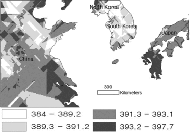
Figure 3. National Institute for Environmental Studies Level 3 product of XCO₂ estimates (unit: ppm) for March to June 2009–2012.

Comparative evaluation of XCO₂ concentrations

As shown in Table 4, the CO₂ distribution varied widely between 395.22 and 382.1 ppm across the study area. The concentration range of CO₂ decreased after the application of kriging and zonal statistics because it tends to be diluted by averaging lower and higher values within administrative regions. The highest and lowest CO₂ concentration levels as derived from the kriging ranged from 388.3 to 394.5 ppm (a difference of 6.2 ppm). The exchange of CO₂ during photosynthesis (uptake) and respiration (release) produces a large diurnal and seasonal impact on observed XCO₂ mixing ratios. Atmospheric CO₂ concentrations have been shown to be associated with surface air temperatures, which is consistent with the hypothesis that warmer temperatures have promoted increases in biosphere activity outside of the tropics [20]. During the spring in NEA, the CO₂ concentration is less affected by the respiration of plants since lower temperatures postpone vegetation greenup. However, with increases in temperature, plant respiration occurs below ground in the roots. Soil respiration also increases, which can emit CO₂ [40]. The CO₂ concentration was higher in southern regions compared to northern regions in the study area because of temperature sensitivity. In addition, the increases in temperature in south NEA occurred more rapidly than in north NEA, which led to higher CO₂ concentrations in south NEA. Using GOSAT data, the author found that the northern region (Shandong, Shanxi of China, South Korea) had lower CO₂ concentrations, while higher concentrations were observed in the southern region (Japan and the Hebei, Anhui and Jiangsu provinces of China).

Table 4. Summary statistics for XCO₂ concentration values after Kriging, and geographic information system zonal statistics (ppm).

	Level 2	Level 3	Zonal statistics
Mean (number of administrative regions)	391.9	392.2	391.3 (27)
Maximum/minimum	95.22 /382.1	397.7/384.1	394.3/387.2
Standard deviation	3.9	2.25	1.7

Because economic performance is extremely differentiated in different regions of NEA, the XCO₂ distribution displayed significant regional differences. Decreasing trends in XCO₂ levels were found in northern parts of central China and South Korea (Figure 4). In contrast, high XCO₂ concentrations were observed in the southeastern (Japan) and southwestern (China) regions, as shown in Figures 3 and 4. High-concentration cities were mostly located in the southern region (Jiangsu–Zhejiang region and Japan; Figure 4), and the concentrations were likely higher in these areas because of intensified human activities in these locations. Three of the five regions with the highest concentration levels were in China, and the remaining two were in Japan (Table 5). Among the 27 administrative regions, Kyushu showed the highest concentration level. These results can be explained largely by the extent of intensified urban and suburban land use in Japan (Kyushu: 394.5 ppm) and the southeastern region of China (Shanghai: 394.1 ppm).

Figure 4. Level 3 XCO₂ concentrations (unit: ppm) for first-level administrative regions (provinces and states) with a temperate climate in Northeast Asia.

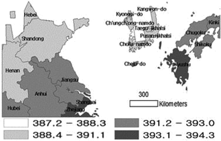
Table 5. Five administrative regions with the highest and lowest XCO₂ concentration levels, ranging from 387.2 to 394.3 ppm.

	Top five cities (XCO2 concentration value)	Bottom five cities (XCO2 concentration value)
1	Kyushu (394.3)	Taegu-jikhalsi (387.2)
2	Shanghai (394.1)	Ch'ungch'ong-namdo (388.7)
3	Zhejiang (393.4)	Cholla-bukto (389.3)
4	Shikoku (393.0)	Kyongsang-bukto (389.3)
5	Jiangsu (392.9)	Kangwon-do (390)

All five administrative regions with the lowest concentration levels were located in South Korea. South Korea, which is one of the most populous countries in the world, is also a major energy user. Rapid economic development, urban expansion and transportation facility development have increased fossil fuel consumption in the last three decades in South Korea, resulting in increased CO₂ concentrations, particularly in cities and industrial areas. However, because the Level 2 XCO₂ data were sparsely sampled in South Korea (see Figure 1), XCO₂ variability could be underestimated in the Level 3 data in comparison to the surrounding well-sampled regions. Also, since only land adjacent to the seashore in South Korea was included in the temperate climate zone (see Figure 4), it is hard to say that CO₂ concentrations in South Korea are lower than those of China and Japan. The approach presented in this paper fails to yield any evidence that area-wide energy consumption and industrial activity in South Korea have influenced recent trends in carbon emissions.

In the southeastern region of China, the industrial use of rural land has increased along with the conversion of both agricultural and forested areas into residential and commercial facilities, particularly along the periphery of large metropolitan areas. In summary, agricultural land use has declined, particularly in the southern region. The world's largest active volcano (Mountain Aso) is in Kyushu, Japan, and there are many other hotspots of tectonic activity including numerous hot springs. Heavy industry is concentrated in the northern part of Fukuoka as well as in the southern region's volcanic area [41]. Volcanic activity and heavy industry have been suggested to be two major factors influencing atmospheric carbon concentrations in Kyushu. Japan was characterized by relatively high concentrations of CO₂ in this study, and this corresponds well with the consistently high levels of industrialization and urbanization as well as volcanic and tectonic activity across the whole country. In Japan, most flat land is urban and built up, which is also consistent with low carbon absorption in those areas. In general, the levels of industrialization and urbanization are distinctly higher in the southern region than in the northern region, and the high CO₂ concentration is correlated with regional energy intensity.

Spatial variations in XCO₂ can also be explained by changes in synoptic transport patterns. High concentrations were observed for the southern part of the study area, possibly due to the presence of atmospheric dust. Asian dust (yellow sand) over continental China and dust or smoke-like phenomena in the some locations in Japan could be contributing factors. Asian dust transforms not only sand dust but also the atmosphere. Matter in the atmosphere can be transferred from northwestern to southeastern China and Japan, which may cause an increased concentration of XCO₂ in the sand dust-covered areas. Atmospheric flow from the north to the south of China and Japan could be the primary reason for increased XCO₂ concentrations in this area.

Fossil fuel burning, atmospheric transport and terrestrial biosphere control processes influence the atmospheric concentrations and variability of CO₂. It is known that terrestrial biospheric fluxes primarily determine the large-scale gradient in XCO₂, and advection of those gradients is the dominant source of synoptic variations in XCO₂ [42]. However, XCO₂ concentrations over industrial regions were detectible with GOSAT data, and the largest anomalies were typically over regions that have large fossil fuel emissions (e.g., the Jiangsu–Zhejiang region of China and the Kyushu region of Japan). These results are consistent with the findings of previous studies showing that changes in observed XCO₂ contrasts could be used to monitor changes in fossil emissions as well as biospheric fluxes. Observations made in China and Korea showed that biospheric fluxes contributed up to 50% of the CO₂ concentrations in polluted regions [21].

Potential and limitations of the Greenhouse Gases Observing Satellite XCO₂ data

Our analysis depends on the quality and distribution of XCO₂ data, but the number of XCO₂ observations was not sufficient for comprehensive monitoring of the study area. There were a total of 222 soundings over 4 years divided between 26 administrative regions. That means that each administrative region had, on average, around nine soundings. These were spread out over 4 years, and were likely spread out unequally in the different regions and through time. Another limitation concerns seasonal variations that were not taken into account because the analysis employed only spring data. Kriging provides only imperfect estimates of XCO₂ concentrations because of a lack of data points. The choice of the temporal resolution used in analyses, meaning the time period over which observations are aggregated, is an important decision in the creation of a Level 3 product [32]. Ideally, Level 3 products are created for the shortest time period possible to minimize the impact of temporal variability. However, this needs to be balanced with a minimum requirement for the number of GOSAT observations. This study generated a Level 3 product by combining spring season observations for 4 years; nevertheless, the values were spaced too far apart to represent the study area in detail. Carbon dioxide maps created over longer time periods will be better able to show the dynamics of regional fossil fuel emission signatures and biospheric fluxes, although even with a large number of measurements, noise due to temporal variability can be expected.

Our XCO₂ estimates cannot separate quantitatively the effect of contributing factors (their retrieval errors and spatial variability in the XCO₂ field) to the estimated XCO₂ distribution at each location [22]. There is still considerable debate about whether GOSAT L2 data have sufficient accuracy. Several studies have compared GOSAT retrieval gas products from different algorithms against TCCON measurements [43,44]. According to the verification results with the FTS SWIR Level 2 product, which was provided by the GOSAT project, the average concentrations of XCO₂ were approximately lower than the validation data by 2–3% [45]. Recently, XCO₂ retrieved using the version 02.xx retrieval algorithm shows much smaller biases and standard deviations (–1.48 and 2.09 ppm for XCO₂) than the version 01.xx data [23]. It has been reported that the bias between GOSAT and ground-based data is a few tenths of a percent for XCO₂ (the GOSAT values are lower), and single-measurement precision is well below 1% [43]. In Hong Kong and Japan, where the two observation stations are located, the monthly average XCO₂ Kriging interpolation data were lower than the ground observation data by 4.8 and 2.2%, respectively [31]. The GOSAT monthly mean data tend to be generally smaller than those from two ground stations in China by 5–10 ppm [46]. The author did not perform a quantitative verification of the retrieved XCO₂ values since variations of GOSAT XCO₂ data were compared with ground-based observations in many previous studies. Therefore, this article assumes that the distribution of XCO₂ data generally is within a 1–5% or 5–10 ppm difference from in situ measurements of XCO₂, as reported in the literature.

The GOSAT XCO₂ data represent the ratio of the total number of CO₂ molecules to the total number of dry air molecules that exist not only close to the Earth's surface, but also in the total vertical column from the surface to the top of the atmosphere. The mechanism of acquiring GOSAT XCO₂ data is based on a column-averaged mixing ratio in the space, while in situ measurements collect site-specific atmospheric mixing ratios from towers, flask sampling onboard aircraft and ships, and fixed-site measurements. Those two quantities cannot be directly compared in terms of carbon concentrations across administrative regions, since the area-wide dry air, column-averaged molar fraction of CO₂ will show quite large differences in values from the atmospheric mixing ratios representing site-specific concentrations. This is particularly true when there are serious geographic variations in the field.

At present, seven different retrieval algorithms exist throughout the world to systematically retrieve global and temporal distributions of gas amounts from the GOSAT data [44,47]. This research used data from the operational NIES version 2 product [23]. There are reasonably large differences between the different retrieval algorithms, which are due to different sorts of systematic biases. If different retrieval algorithms had been applied, Kyushu might not have been the region with the highest concentration. A critical concern in model-based estimates of carbon flux is their reliability in the presence of uncertainties in the input data and in their representation of biogeochemical processes. In fact, the SWIR channels of GOSAT measure the column-averaged CO₂ concentration, or XCO₂, rather than some local or surface-level concentration. The column XCO₂ is not very sensitive to local fluxes, but more sensitive to very large-scale (tens of thousands of kilometers) fluxes, depending on how these are convolved with the global transport [42]. Recently, there has been some progress in looking at regional XCO₂ contrasts to estimate city-level emissions [48], but these studies must be set up extremely carefully.

Conclusion

To overcome data availability challenges in accounting carbon concentration, exploration of high-resolution remote-sensing data offers insight. The author feels that this article starts to develop ideas of how to quantify CO₂ concentrations across administrative regions in a usable way within a consistent framework. The author hopes that this contribution will initiate the needed conversation that will drive the development of foundational theory to deal with uncertainty and time issues in accounting carbon concentration. While not complete as a finished methodology, the author sees the possibility for the basic approach to be adopted in GHG emission reporting in the coming years, since this research presented carbon concentration map from actual data of a real case-study area. The author does not suggest that satellite observations are the sole answer to resolving uncertainty in administrative region-wide carbon concentration, nor does he believe that they will obviate the need for in situ measurements. On the contrary, field measurements of carbon concentration are essential for both calibrating and validating (i.e., assessing) spatial estimates of carbon concentration derived from satellite observations. This is particularly true when the satellite and field data are linked across scales using datasets judiciously acquired from Geographic boundary limited accounting.

There is considerable uncertainty in quantifying CO₂ concentrations at the level of administrative regions, because bottom-up field sampling monitors only a fraction of the area of interest and top-down biospheric models simplify complex real-world processes with a great deal of uncertainty. The GOSAT Level 3 XCO₂ products used in this study, which were obtained from kriging, allowed for an examination of whether carbon concentrations varied according to the administrative regions. This paper contributes to the literature by presenting comparable carbon concentration maps across administrative regions with a temperate climate. Results revealed marked geographical variation in carbon concentrations with higher values in industrial regions and lower values in rural communities; concentrations ranged from 394.3 to 387.2 ppm. Although further research is required, the results provide the initial methodological framework for examining carbon concentration patterns in the context of regional and local communities.

Given the large range of possible common environmental drivers such as fossil fuel use, biophysical flux and synoptic transport patterns, there are limitations to quantifying their contribution to the total XCO₂. The proposed method for identifying carbon concentrations in administrative regions has yet to be tested over more diverse regional-scale land surface conditions (e.g., tropical and dry climates), and the approach used here that was constrained to a specific climate region (temperate climates) needs to be more thoroughly validated through further research to better understand the spatially integrative relationships between carbon concentrations and climate conditions. Overall, this paper constitutes an early effort to comprehensively investigate carbon concentrations across administrative regions with different type of climates.

Acknowledgements

The author thanks the members of the GOSAT Project (JAXA, NIES and Ministry of the Environment Japan) for providing the GOSAT Level 2 product. The author also thanks ESRI for providing a world administrative divisions map. Thanks are extended to the Institute for Veterinary Public Health for sharing a world map of the Köppen-Geiger climate classification for this project.

References

- Reynolds DR, McNulty ML. On the analysis of political boundaries as barriers: a perceptual approach. East Lakes Geogr. 4, 21–38 (1968).
- Leimgruber W. The perception of boundaries: barriers or invitation to interaction? Reg. Basil. 30(2), 49–59 (1989).
- Erickson P, Lazarus M, Chandler C, Schultz S. Technologies, policies and measures for GHG abatement at the urban scale. Greenh. Gas Measure. Manage. 3(1-02), 37–54 (2013).
- Feiock RC, Bae J. Politics, institutions and entrepreneurship: city decisions leading to inventoried GHG emissions. Carbon Manage. 2(4), 443–453 (2011).
- Lo K. Urban carbon governance and the transition toward low-carbon urbanism: review of a global phenomenon. Carbon Manage. 5(3), 269–283 (2014).
- Kennedy C, Steinberger J, Gasson B et al. Methodology for inventorying greenhouse gas emissions from global cities. Energy Policy 38(9), 4828–4837 (2010).
- Sovacool BK, Brown MA. Twelve metropolitan carbon footprints: a preliminary comparative global assessment. Energy Policy 38(9), 4856–4869 (2010).
- Wright LA, Coello J, Kemp S, Williams I. Carbon footprinting for climate change management in cities. Carbon Manage. 2(1), 49–60 (2011).
- Sippel M. Urban GHG inventories, target setting and mitigation achievements: how German cities fail to outperform their country. Greenh. Gas Measure. Manage. 1(1), 55–63 (2011).
- United Nations Environment Programme (UNEP), UN-Habitat, Bank W. Draft International Standard for Determining Greenhouse Gas Emissions for Cities. Rio de Janeiro, Brazil (2010).
- ICLEI. International Local Government GHG Emissions Analysis Protocol (IEAP), Version 1.0. (2009). International Council for Local Environmental Initiatives, United Nations, New York.
- Dhakal S, Shrestha RM. Bridging the research gaps for carbon emissions and their management in cities. Energy Policy 38(9), 4753–4755 (2010).
- Marland E, Cantrell J, Kiser K, Marland G, Shirley K. Valuing uncertainty part I: the impact of uncertainty in GHG accounting. Carbon Manage. 5(1), 35–42 (2014).
- Chavez A, Ramaswami A. Progress toward low carbon cities: approaches for transboundary GHG emissions' footprinting. Carbon Manage. 2(4), 471–482 (2011).
- Grimmond CSB, King TS, Cropley FD, Nowak DJ, Souch C. Local-scale fluxes of carbon dioxide in urban environments: methodological challenges and results from Chicago. Environ. Pollut. (116), S243–S254 (2002).
- Velasco E, Pressley S, Allwine E, Westberg H, Lamb B. Measurements of CO2 fluxes from the Mexico city urban landscape. Atmos. Environ. 39, 7433–7446. (2005).
- Tian X, Chang M, Shi F, Tanikawa H. How does industrial structure change impact carbon dioxide emissions? A comparative analysis focusing on nine provincial regions in China. Environ. Sci. Policy 37(0), 243–254 (2014).
- Al-mulali U, Sheau-Ting L. Econometric analysis of trade, exports, imports, energy consumption and CO2 emission in six regions. Renew. Sustain. Energy Rev. 33(0), 484–498 (2014).
- NEASPEC (North-East Asian Subregional Programme for Environmental Cooperation). Activity plan of eco-efficiency partnership in North-east Asia. In: The 14th Senior Officials Meeting (SOM) of NEASPEC (North-East Asian Subregional Programme of Environmental Cooperation). NEASPEC, Moscow, Russian Federation (2009). This paper has been reproduced as submitted by the Secretariat (issued without formal editing).
- Myneni RB, Keeling CD, Tucker CJ, Asrar G, Nemani RR. Increased plant growth in the northern high latitudes from 1981 to 1991. Nature 386, 698–701 (1997).
- Turnbull JC, Tans PP, Lehman SJ et al. Atmospheric observations of carbon monoxide and fossil fuel CO2 emissions from East Asia. J. Geophys. Res. Atmos. 116(D24), D24306 (2011).
- Hammerling D. M., Michalak A. M., O'Dell C, Kawa SR. Global CO2 distributions over land from the Greenhouse Gases Observing Satellite (GOSAT). Geophys. Res. Lett. 39(8), L08804 (2012).
- Yoshida Y, Kikuchi N, Morino I et al. Improvement of the retrieval algorithm for GOSAT SWIR XCO2 and XCH4 and their validation using TCCON data. Atmos. Measure. Tech. 6(6), 1533–1547 (2013).
- Yokota T, Yoshida Y, Eguchi N et al. Global concentrations of CO2 and CH4 Retrieved from GOSAT: first preliminary results. Sci. Online Lett. Atmos. 5, 160–163 (2009).
- Lloyd J, Taylor JA. On the temperature dependence of soil respiration. Rev. Funct. Ecol. 8, 315–323 (1994).
- Boone RD, Nadelhoffer KJ, Canary J. D., Kaye J. P. Roots exert a strong influence on the temperature sensitivity of soil respiration. Nature 396, 570–572 (1998).
- Welp LR, Keeling RF, Meijer HA et al. Interannual variability in the oxygen isotopes of atmospheric CO2 driven by El Nino. Nature 477(7366), 579–582 (2011).
- Kottek MJ, Grieser C, Beck B, Rubel F. World map of the Köppen–Geiger climate classification updated. Meteorol. Z. 15, 259–263 (2006).
- Rubel F, Kottek M. Observed and projected climate shifts 1901–2100 depicted by world maps of the Köppen–Geiger climate classification. Meteorol. Z. 19(2), 135–141 (2010).
- Environmental System Research Institute (ESRI). ArcGIS Software Help Menu (Spatial Analysis Toolbox). ESRI (2010). Redlands, CA.
- Liu Y, Wang X, Guo M, Tani H. Mapping the FTS SWIR L2 product of XCO2 and XCH4 data from the GOSAT by the Kriging method? A case study in East Asia. Int. J. Remote Sens. 33(10), 3004–3025 (2011).
- Hammerling D. M., Michalak A. M., Kawa SR. Mapping of CO2 at high spatiotemporal resolution using satellite observations: global distributions from OCO-2. J. Geophys. Res. Atmos. 117(D6), D06306 (2012).
- Goovaerts P. Geostatistics for Natural Resources Evaluation. Oxford University Press, New York, NY, USA (1997).
- Um JS, Choi JH. Comparative evaluation among different kriging techniques applied to GOSAT CO2 map for North East Asia. J. Korean Environ. Impact Assess. 20(6), 1–10 (2011).
- Um JS, Choi JH. Comparative evaluation for seasonal CO2 flows tracked by GOSAT in Northeast Asia. J. Korea Spat. Inf. Soc. 20(5), 1–13 (2012).
- Um JS, Choi JH. Evaluating cross-correlation of GOSAT CO2 concentration with MODIS NDVI patterns in North-east Asia. J. Korea Spat. Inf. Soc. 21(5), 15–22 (2013).
- Um JS, Choi JH. Analysis of CO2 distribution properties using GOSAT: a case study of North-east Asia. J. Korea Geospat. Inf. Soc. 21(2), 85–92 (2013).
- Isaaks EH, Srivastava RM. An Introduction to Applied Geostatistics. Oxford University Press, New York, NY, USA (1989).
- Deutsch CV, Journel AG. Gslib: Geostatistical Software Library and User's Guide. Oxford University Press, New York, NY, USA (1998).
- Tang XL, Zhou GY, Liu SG et al. Dependence of soil respiration on soil temperature and soil moisture in successional forests in southern China. J. Integr. Plant Biol. 48(6), 654–663 (2006).
- Cobbing A. Kyushu: Gateway to Japan. Global Oriental (2008). Folkestone, UK.
- Keppel-Aleks G, Wennberg PO, Schneider T. Sources of variations in total column carbon dioxide. Atmos. Chem. Phys. 11(8), 3581–3593 (2011).
- Butz A, Guerlet S, Hasekamp O et al. Toward accurate CO2 and CH4 observations from GOSAT. Geophys. Res. Lett. 38(14), L14812 (2011).
- Oshchepkov S, Bril A, Yokota T et al. Effects of atmospheric light scattering on spectroscopic observations of greenhouse gases from space. Part 2: algorithm intercomparison in the GOSAT data processing for CO2 retrievals over TCCON sites. J. Geophys. Res. Atmos. 118(3), 1493–1512 (2013).