Spatial effect of factors affecting household CO₂ emissions at the provincial level in China: a geographically weighted regression model

ABSTRACT

The size of household CO₂ emissions (HCE) has drawn increasing attention recently. Due to differences in geographical location, traditional models do not provide a valid basis or countermeasures for CO₂ emissions reduction in different provinces, leading to biased estimation. This paper uses a geographical weighted regression (GWR) model to examine the spatial effect of urbanization, energy intensity, energy structure and income on HCE. The results indicate an obvious spatial effect on carbon emissions in the provinces. The impact of urbanization on household CO₂ emissions presented an increasing trend from the southeastern coast to the northwest from 2000 to 2015. Energy intensity had a remarkably positive effect on HCE in 2000 and 2015, although it had a negative effect in all provinces in 2005 and in some provinces in 2010. The elasticity coefficient of energy structure on HCE was negative in most provinces in all four years, indicating that more use of natural gas and electricity decreased HCE. Income was a powerful explanatory factor for growth in household CO₂ carbon emissions in all years. The effect of income on HCE was positive and showed an increasing tendency year by year.

KEYWORDS:

• spatial differences
• GWR
• CO₂ emissions
• household

Introduction

The rise in greenhouse gas (GHG) emissions, especially carbon dioxide emissions, has posed a tremendous threat to the development of the global economy and society. China became the world's largest CO₂ emitter in 2006, and will continue its rapid economic expansion with increasing energy consumption and emissions [1]. Current studies have focused mainly on energy consumption and carbon emissions in the industrial sector and have paid insufficient attention to the household sector. In some developed countries, household energy consumption has exceeded industrial energy consumption and accounts for the majority of energy use [2]. Household energy consumption has continued to increase in recent decades and creates 72% of GHG at the global level [3,4]. Final energy consumption in the household sector in accounts for 20.4% of total final energy consumption, and CO₂ emissions were 343.9 million tons oil equivalent (Mtoe) in 2014 [5,101].

With rapid industrialization and urbanization, population growth, and improvement in people's living standards, household energy consumption and carbon emissions in China have shown sustained high growth. A growing number of residents in China prefer to spend more money on improving their quality of life and enjoying a high-carbon lifestyle [6–8]. The increase in household consumption has made a large contribution to the growth of energy consumption and CO₂ emissions [9,10]. Furthermore, household carbon emissions show obvious spatial variation [11]. Under international pressure for CO₂ emissions reduction, the Chinese government made a commitment that it would achieve peak CO₂ emissions around 2030 and reduce its carbon intensity by 60–65% in 2030 compared to 2005 [12]. To achieve this carbon emissions reduction goal, specific attention should be paid to investigating carbon emissions in the household sector.

Many studies have shown that household energy consumption is closely related to CO₂ emissions [13–15]. Plenty of studies have focused on household CO₂ emissions from the perspective of production [16,17] and consumption [18,19]. Lenzen et al. [20] evaluated sustainable household consumption from a global perspective by input–output analysis and found that energy requirements vary from one country to another. Reddy and Srinivas [21] studied the energy consumption pattern in the household sector and analyzed the causalities underlying present usage patterns. Based on the consumer lifestyle approach (CLA), Bin and Dowlatabadi [22] examined the relationship between consumer activities and energy use and related CO₂ emissions. The results revealed that 80% of energy use and CO₂ emissions in the United States can be attributed to consumer demands and related economic activities.

The impact of household CO₂ emissions can be divided into direct and indirect impacts. Weber and Perrels [23] investigated household direct and indirect energy demand and CO₂ emissions in West Germany, France and the Netherlands. Using the logarithmic mean Divisia index (LMDI) decomposition method, Zha et al. [24] found that energy intensity decreased direct household CO₂ emissions and that income increased the direct emissions in both urban and rural China. Zang et al. [25] also used the LMDI to examine household-related driving factors behind household direct carbon emissions, and found that per-capita household income and number of households contributed to increasing household direct carbon emissions. Many studies have found that indirect energy consumption is much higher than direct energy consumption [26–28]. Based on the CLA, Wang and Yang [2] estimated the net primary productivity (NPP) and energy ecological footprint (EEF) of indirect energy consumption. Their results showed that the EEF of indirect energy use was on the rise for urban residents, but declined for rural residents. Furthermore, the study examined the effects of urbanization level, economic level, Engel coefficient, energy intensity and industrial structure on indirect energy consumption using the STIRPAT (Stochastic Impacts by Regression on Population, Affluence, and Technology) model. Yuan et al. [29] investigated regional variations in the impacts of urbanization, consumption ratio and consumption structure on residential indirect CO₂ emissions in China using a new structural decomposition analysis (SDA) model. The results showed that urbanization and consumption structures play important roles in the growth of residential indirect emissions. Li et al. [1] found that total CO₂ emissions from urban households were higher than those from rural households using the input–output (I–O) model. A unidirectional causal relationship was found to exist between urbanization and both direct and indirect household CO₂ emissions. Tian et al. [30] calculated household carbon footprints in Liaoning Province and showed that indirect carbon footprints were larger than direct carbon footprints. Duarte et al. [31] used the I–O model and the social accounting matrix (SAM) and found that a positive relationship existed between average carbon emissions and household income in Spain. Lyons et al. [32] indicated that household indirect carbon emissions increased sharply with increasing household income in Ireland using the I–O model.

A number of studies have analyzed the factors affecting household carbon emissions. Das and Paul [33] analyzed CO₂ emissions from household consumption in India in 1993–1994 and 2006–2007. Wang and Liu [34] examined the factors that influenced household daily travel CO₂ emissions in Beijing based on a decomposition analysis model. Liu et al. [9] analyzed the impact of household consumption on carbon emissions in China's urban and rural regions using the I–O model. Many significant factors affecting household carbon emissions have been identified, such as urbanization [25], energy intensity [35], income [32,36,37], household size [38,39], ownership of assets, and individual cognition and household lifestyle [40]. Most of the previous literature investigated factors influencing household energy consumption and emissions based on various methods. Among these, the LMDI is a commonly used decomposition method for analyzing the influencing factors of carbon emissions. The results are easy to explain with a sound theoretical foundation and no residuals [41]. However, the decomposition factors are limited by the LMDI method. The STIRPAT model is used to analyze the impacts of population, affluence and technology on carbon emissions. This model is derived from the IPAT model and allows other impact factors to be added to analyze their influence on environmental pressure [42]. It is widely used to solve realistic environmental problems that combine social, economic and technological factors [43]. Due to the two-way feedback between household consumption and emissions, the I–O model can consider only the impact from production [10]. Because of differences in geographical location, the relationship between variables and model structure will change accordingly. The geographically weighted regression (GWR) model allows the estimated parameters to vary across regions, making it possible to assess potential spatial differences. Xu et al. [44] investigated the driving forces of CO₂ emissions in the manufacturing industry using a GWR model. Xu and Lin [45] used a GWR model to investigate the differential effects of various factors on CO₂ emissions in the agricultural sector and found that the impacts were homogeneous across countries. Videras [46] explored the geographical variability of CO₂ emissions using a GWR model and found strong evidence of spatial heterogeneity in the estimated elasticities of emissions. These existing studies indicate that the GWR model is considered the most appropriate to estimate parameters in CO₂ emissions studies [47].

The innovation and contribution of this study mainly lies in the following two aspects. First, previous studies have analyzed the factors affecting household CO₂ emissions based on various methods, such as the ordinary least squares (OLS), LMDI, STIRPAT and I–O models. However, traditional models cannot consider spatial location, which leads to biased estimation. As a result, valid bases and countermeasures for CO₂ emissions reduction in each region cannot be provided. Actually, from a spatial point of view, it is worth noting that spatial heterogeneity and dependence exist at the provincial level. On the one hand, China is a vast country, with significant provincial differences in economic development, urbanization and energy intensity. The imbalance of economic development is caused by large provincial differences in household consumption and emissions by residents in China. The effects of carbon emissions vary substantially among different provinces due to significant differences in resource structure and infrastructure [48]. On the other hand, the environments of neighboring provinces influence each other and are interlinked and interactive. These differences and similarities are caused mainly by the geographical locations and carbon emissions characteristics of the provinces. Second, although some researchers have analyzed the impact factor on CO₂ emissions by spatial analysis, most of them focus on the industrial sector, agriculture sector, manufacturing sector, etc. Spatial effects on impact factors for household CO₂ production in adjacent regions have not received the attention they deserve. To promote residential energy conservation and carbon emissions reduction effectively and directly, it is critical to consider spatial effects in different provinces in the study of CO₂ emissions. Therefore, this study has used a GWR model to examine the impacts of urbanization, energy intensity, energy structure and income on household CO₂ emissions, and to reveal regional variability and correlations in emissions elasticity. The objective was to develop pertinent policy suggestions according to the characteristics of household carbon emissions in different provinces.

The remainder of this paper is structured as follows. The next section describes the methodology of the GWR model, Moran's index and the data sources. The third section presents results and discussion, and conclusions and policy implications are summarized in the fourth section.

Methodology and data

Spatial correlation index

Analysis of spatial autocorrelation should be conducted before the GWR model. Spatial autocorrelation is measured by Moran's index (Moran's I), which is the most commonly used method. It is chosen to represent the spatial correlation of the household CO₂ emissions. The formula for Moran's I is as follows [49]:(1) where is the observation in the ith province, is the observation in the jth province and is the spatial weight of matrix. is equal to 1 when province i and province j are adjacent; otherwise, is equal to 0. represents the mean of (i = 1, 2,…, n) or (j = 1,2,…, n). n is the total number of provinces.

The values of Moran's I are between − 1 and 1. If Moran's I < 0, there is negative spatial correlation among the spatial units. If Moran's I > 0, it means that there is a positive spatial correlation, and the values of similar properties in the geospatial distribution tend to gather in one area [50]. If Moran's I = 0, this indicates no spatial relationship. That is to say, the larger this value, the stronger the correlation.

Geographical weighted regression model

The GWR model was first proposed by Brunsdon et al. [51] and takes different spatial locations into consideration. Because the model can easily examine and identify patterns by calculating local statistics and spatial relationships between variables [52], it is mainly used in the fields of real estate, agriculture and economics. The GWR model can easily examine and identify patterns by calculating local statistics and spatial relationships between variables [52]. The GWR technique takes into account various geographic phenomena, providing data that can be communicated to potentially affected people, as well as to government agencies considering policies to reduce exposure and adverse effects [53–55]. Many studies have demonstrated that spatial analysis using a GWR model can provide a reliable reference for regional policymaking [56,57]. China has a vast territory, with significant provincial spatial differences in household energy consumption. Due to differences in geographical location, the relationship between the variables and model structure will change accordingly. CO₂ emissions, as a kind of atmospheric resource, will obviously vary with changes in geographical location. Therefore, the GWR model provides improved explanatory power and is considered to be more appropriate than other methods to explore spatial differences in household CO₂ emissions. Actually, GWR is an extension of the general linear regression model and includes the spatial attributes of the data [47]. The equation is:(2) where represents the dependent variable for observation i, and stands for the spatial coordinates of the ith region. is a function of the geographical position, which donates the kth regression coefficient in the ith region.

The parameters of each observation can be estimated using the spatial weighting function. The Gaussian kernel function is one of the most popular functions applied to the GWR model and it produces weights that monotonically decrease with distance. The Gaussian kernel function is an exponential function, and its equation is:(3) where is the weight for data at observation j in the model estimated for observation I, is the distance between observation i and j, and b is the kernel bandwidth. If i is observed, the weight of other points will be decreased with the increase of distance based on the Gauss curve. It is very important to choose the appropriate bandwidth to establish the weight function. In general, the most widely used methods are the Akaike information criterion (AIC) and cross validation (CV) [58]. In order to determine the appropriate bandwidth b, a cross validation method (CV) can be used, it was proposed by Bartholomew [58]. The relationship between b and CV is:(4) where n is the number of observations, and is the estimated value of . When the CV reaches the minimum, the corresponding b is the appropriate bandwidth.

However, different bandwidths could be obtained by different weighting methods, and most studies choose AIC as the calculation criterion. It is a selection criterion through the estimation of the parameters based on the maximum likelihood principle. Optimization of specific weight function bandwidth has a great influence on the accuracy of the GWR model. Therefore, an adaptive kernel function was used to obtain the optimal bandwidth and minimize the corrected AIC [59].

Some researchers have shown that urbanization, energy intensity and energy structure are the important driving forces for household CO₂ emissions [60,61]. In addition, other factors such as household size, age structure, income, education level, ownership of assets, individual cognition and household lifestyle also impact household consumption and CO₂ emissions [40]. However, GWR models must be applied to variables with low correlation. This study tried to select urbanization, energy intensity, energy structure, household size, age structure and education level according to the accessible data. Serious multicollinearity was found to exist among these variables, and a GWR result could not be obtained. Therefore, urbanization, energy intensity, energy structure and income were used to estimate the spatial effects of household carbon emissions by the GWR model. The regression model is as follows:(5) where denotes the spatial coordinates of the ith province (i = 1, 2, 3,…, 30). is a function of the geographical position, which indicates the kth regression coefficient in the ith province. In this study, household CO₂ emissions (HCE) is selected as dependent variable. URB is the urbanization level, which is represented by the proportion of the urban population and the total population. EI stands for the technology level, which is measured by energy intensity (expressed as total energy use divided by gross domestic product, GDP). ES indicates the energy structure and is expressed as the percentage of coal cosumption and total energy consumption. IC represents income level, which indicates the disposable income of residents. is the residual.

Data source

In this paper, 30 provinces, autonomous regions and municipalities of China were chosen as the research object to examine the spatial difference in CO₂ emissions. The study used the cross-sectional data in 2000, 2005, 2010 and 2015 to analyze the spatial difference of influencing factors of carbon emissions, and to further study the changes of four variables in each year.

This study considers the direct household CO₂ emissions caused by direct energy consumption, such as the energy used for lighting and heating. In the calculation of direct household carbon emissions, 13 kinds of energy related to household consumption were calculated, including raw coal, other washed coal, briquettes, coke, coke oven gas, other gas, gasoline, kerosene, diesel oil, liquefied petroleum gas, natural gas, heat and electricity. The direct household CO₂ emissions are calculated according to the formula of CO₂ emissions in the Intergovernmental Panel on Climate Change [62]. The data on energy consumption and energy structure are calculated based on the China Energy Statistical Yearbook 2001, 2006, 2011 and 2016 [63]. The data on urbanization and income are collected from China Statistical Yearbook 2001, 2006, 2011 and 2016 [64]. Energy intensity is expressed as energy consumption divided by GDP. To eliminate the interference of price fluctuations, the data of GDP and income are converted into 2000 constant price (RMB).

Results

Spatial distribution of household energy consumption in urban and rural areas

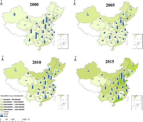
Figure 1 shows total household energy consumption and the proportions of urban and rural consumption. Total household energy consumption increased year by year as a result of rapid urbanization and changes in residents’ lifestyles. The spatial distribution of household energy consumption shows that provinces in the eastern and central regions had significantly higher energy consumption than those in the western region. Hebei, Liaoning and Guangdong had higher energy consumption than other provinces in 2000. In 2005, Liaoning and Shandong Provinces had the highest energy consumptions and produced 1552.25 × 10⁴ tons and 1498.55 × 10⁴ tons, respectively. The energy consumption of Shandong Province in 2010 was the largest (2004.99 × 10⁴ tons). In 2014, Guangdong, Hebei and Shandong had the highest energy consumption (2932.33× 10⁴ tons, 2715.25× 10⁴ tons, and 2370.06 × 10⁴ tons respectively). From a comparison of urban and rural areas, various parts of Tianjin, Inner Mongolia, Liaoning, Heilongjiang and Guangdong had the largest gaps in household energy consumption in the whole country, and these gaps increased yearly.

Figure 1. Urban and rural direct household energy consumption of China in 2000, 2005, 2010 and 2015.

Spatial distribution of household energy consumption structure

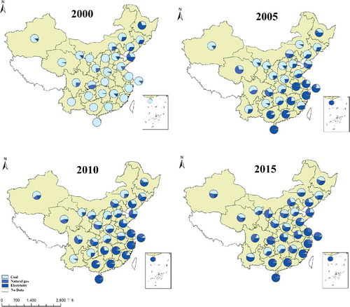
According to statistics, coal, natural gas and electricity are the main energy sources in household energy consumption. Figure 2 shows the structure of household energy consumption in the four years studied and indicates that the proportion of coal decreased, whereas the proportions of natural gas and electricity increased from 2000 to 2015. Specifically, in 2000 and 2005, the proportion of coal in energy consumption accounted for almost 50% in most provinces, and the proportion in Shanxi, Inner Mongolia, Guizhou, Gansu, Ningxia and Xinjiang Provinces was over 80%. The proportion of electricity was lower than the proportion of coal. However, the proportion of electricity was greater than 90% in Zhejiang, Anhui and Hainan Provinces. The proportion of natural gas was relatively low in 2005, except for Beijing, Tianjin, Sichuan and Chongqing, each of which had a proportion greater than 20%. In 2010 and 2015, the proportion of coal decreased in most provinces; in particular, the figure for Shanxi Province dropped below 70% in 2011. At the same time, the proportions of natural gas and electricity rapidly increased. As a primary energy source, natural gas contains fewer impurities and has a significant positive effect on environmental protection. Therefore, the government has encouraged residents to use natural gas and has gradually reduced the proportion of coal. By 2015, the proportion of coal in all provinces had dropped to 30%. In addition to Inner Mongolia, Guizhou and Gansu Provinces, other provinces had dropped below 50% coal use. The proportion of electricity increased to 50%, and the proportion of natural gas increased to 20%. In particular, Chongqing increased to 50%.

Figure 2. Household energy consumption structure of China in 2000, 2005, 2010 and 2015.

Spatial autocorrelation analysis

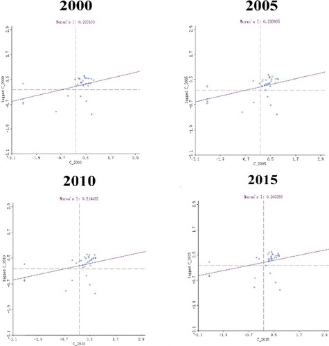
Spatial autocorrelation should be analyzed before using the GWR model for regression estimation. Figure 3 presents a Moran scatter plot using the Open GeoDa software, which shows that most provinces are concentrated in the first and fourth quadrants. The Moran I values in 2000, 2005, 2010 and 2015 were 0.235, 0.231, 0.214, and 0.203, respectively. These values indicate that household CO₂ emissions have a spatial correlation in different provinces. This correlation gradually decreased from 2000 to 2015, which shows that the differences in spatial distribution of provincial household CO₂ emissions are growing.

Figure 3. Moran scatter plot of household CO₂ emissions in 2000, 2005, 2010 and 2015.

Results of the GWR model

Table 1 illustrates the estimated result of the impact on household CO₂ emissions in 2000, 2005, 2010 and 2015, calculated using ArcGIS 10.3 software. As shown, the local R² of the GWR model in the four years is 0.914, 0.929, 0.920 and 0.994, respectively. Taking the result of 2005 as an example, the local R² value for the GWR model (R² = 0.914, adjusted R² = 0.892) indicates that 91.4% of the impact of household CO₂ emissions can be explained by urbanization, energy intensity, energy structure and income. GWR estimation of each local model is determined endogenously through a process that selects the number of neighbors, and consequently the bandwidth, that minimizes the AIC [46]. AICc is used to reflect the goodness of fit for the model. The smaller the AICc values, the better the model performed [54]. Table 1 shows that the GWR has a smaller AICc in each year. As a consequence, the higher R² and lower AICc suggest that GWR has stronger ability to explain the impacts of household CO₂ emissions. Due to the difference in geographical position, the relationship between variables and the structure of the model will change accordingly. Therefore, the GWR model provides improved explanatory power and is considered to be more appropriate than other models to explore the spatial effect of household CO₂ emissions.

Table 1. Comparison of OLS model and geographical weighted regression (GWR) model.

	OLS model				GWR model
	2005	2008	2011	2014	2005	2008	2011	2014
Local R^2	0.971	0.979	0.984	0.986	0.977	0.985	0.985	0.986
Adjusted R^2	0.966	0.976	0.981	0.983	0.969	0.979	0.982	0.984
Bandwidth	–	–	–	–	34.808	27.664	47.501	85.308
Akaike Information Criterion (AICc)	45.917	37.648	31.244	28.525	44.377	35.817	31.030	28.190
Population (P)	0.951	1.060	1.111	1.191	0.952	1.055	1.108	1.189
Urbanization(URB)	1.597	1.848	1.859	1.914	1.631	1.837	1.859	1.921
Energy Intensity (EI)	0.760	0.692	0.719	0.568	0.719	0.608	0.682	0.554
Energy Structure (ES)	0.070	0.005	0.031	0.100	0.055	0.030	0.040	0.103
Income (IC)	−0.393	−0.704	−0.933	−1.282	−0.360	−0.666	−0.907	−1.263

Discussion

Urbanization

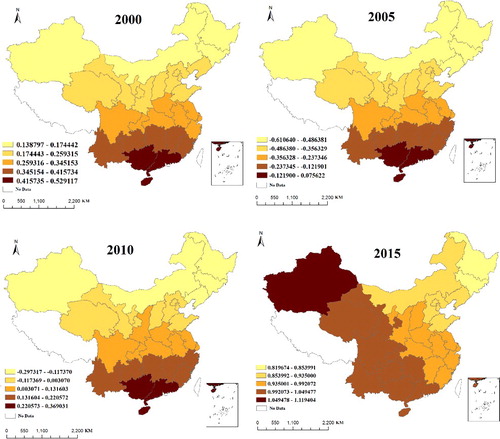
Figure 4 shows the estimated results of the effects of urbanization on household CO₂ emissions. In 2000, urbanization increased CO₂ emissions with an elasticity from 0.034 to 0.297. The regression coefficient of urbanization on household CO₂ emissions in 2005 was between 0.270 and 0.989. In 2010, urbanization increased emissions with a coefficient from 0.585 to 1.255, indicating that rapid urbanization was conducive to increasing CO₂ emissions. Compared to 2010, the impact on household CO₂ emissions decreased in 2015, with a coefficient from 0.065 to 0.835. Specifically, the impact of urbanization on household CO₂ emissions showed an increasing trend from the southeastern coast to the northwest from 2000 to 2015. This may be attributed to the fact that household energy consumption in the northwest has increased rapidly with urbanization in recent years. The demand for urban infrastructure and the regional transportation network continued to expand with the rapid growth of the urban population, leading to more direct carbon emissions [65]. In addition, extensive expansion of urban areas has attracted a large number of rural residents to live in cities, embracing the urban lifestyle and changing their consumer demands and behavior in this process. This change has boosted direct and indirect energy consumption and CO₂ emissions. At present, due to excessive expansion of large and ‘super’ cities with urbanization, life energy efficiency is difficult to maintain with the cost of rapidly expanding transportation and infrastructure maintenance. At the same time, residential energy consumption tendencies and the negative externalities of city life eventually lead to a rise in energy consumption per capita.

Figure 4. Regression coefficients of urbanization for 2000, 2005, 2010 and 2015.

Energy intensity

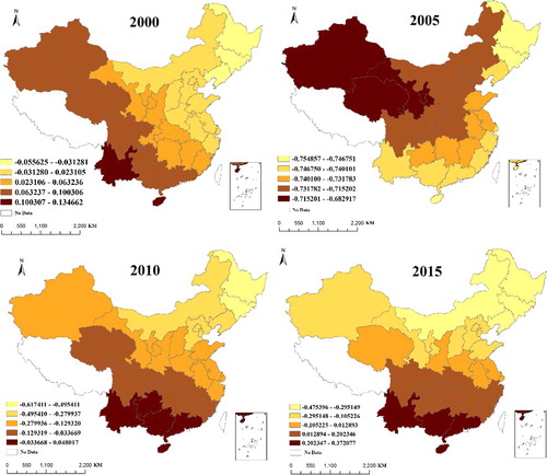
Energy intensity represents energy consumption per unit GDP, which reflects the impact of technology on carbon emissions. A decrease in energy intensity implies that technology is playing a positive role in emissions reduction. Figure 5 reveals that energy intensity had a positive effect on household CO₂ emissions in all provinces from 2000 to 2015. The estimated result conforms to the research results presented by Zhang [66] and He et al. [67]. The effect of energy intensity on carbon emissions reduction has shown regional differences in different years. The influence in 2000 was mainly concentrated in the southern provinces, but in 2015, it was mainly concentrated in the west. This could be due to the fact that the level of technology varies greatly in different regions and its effect on household CO₂ emissions reduction is unstable. Actually, compared to other countries, technological progress in energy intensity in China has been relatively slow. However, it had a negative effect in all provinces in 2005 and in some provinces in 2010. The effect of technological progress can be offset by rapid increases in energy consumption [68]. In other words, an energy rebound effect may occur. The energy rebound effect is the phenomenon in which a new technology designed to improve energy efficiency stimulates consumers and producers to use more energy, leading to more energy consumption instead of less [69]. Therefore, to achieve the goal of carbon emissions reduction, it is not enough to improve energy consumption efficiency alone. Other efforts such as industrial structural adjustments and energy structure optimization are also needed.

Figure 5. Regression coefficients of energy intensity for 2000, 2005, 2010 and 2015.

Energy structure

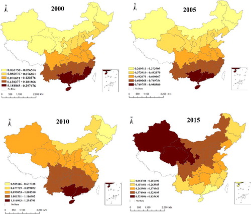
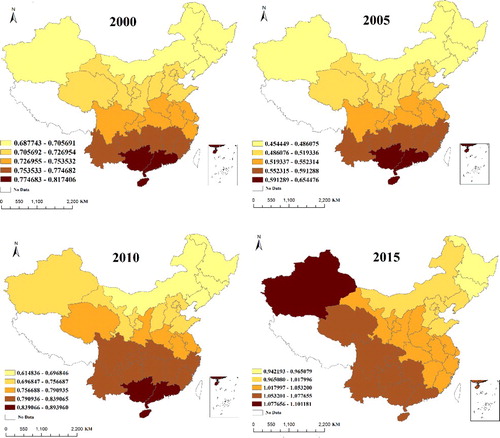
Figure 6 reveals the effect of energy structure on household CO₂ emissions in the four years studied. The energy structure is represented by the proportion of natural gas and electricity consumption to total energy consumption. As shown, the elasticity coefficient of the influence of energy structure on household CO₂ emissions is negative in most provinces in the four years, indicating that energy structure decreases household CO₂ emissions. However, energy structure increased household CO₂ emissions in some provinces in 2000 and 2015. Compared with other variables, the explanatory power of energy structure for carbon emissions is relatively low. In 2000 and 2005, its influence was mainly concentrated in northwestern China, but it expanded to the south in 2010 and 2015. Although China has optimized its energy consumption structure in recent years, the effect of energy structure adjustment on carbon emissions reduction has been relatively low [70]. This may be attributed to the fact that the amount of coal consumed for winter heating in the north is higher than in the south of China. Most importantly, coal reserves are mainly distributed in the north, which leads to more coal consumption and more emissions in the north. The energy consumption structure of the south is dominated by natural gas and electricity consumption, a structure that will decrease household CO₂ emissions.

Figure 6. Regression coefficients of energy structure for 2000, 2005, 2010 and 2015.

Income

Figure 7 shows that income is a powerful explanatory factor for household CO₂ emissions growth in all four years studied. The effect of income on household CO₂ emissions is positive and shows an increasing tendency year by year, which means that income growth exerted a strong upward pressure on household CO₂ emissions. The result is consistent with the conclusions of Coondoo and Dinda [71], Jun et al. [72], and Golley and Meng [73]. The range of influence was mostly concentrated in central and southern China from 2000 to 2010. With increasing disposable income, households in these regions have higher consumption capacity and prefer to consume more carbon-emitting products. In 2015, this influence expands from the southwestern to the northeastern parts of China. The income gap among northern, central and western regions is broadening. This excessive inequality positively affects household energy demand and increases household consumption and CO₂ emissions. Household-based consumption demand exceeds individual-based demand, which directly promotes expansion of the scale of residents’ consumption and causes more emissions [74]. Moreover, the development of environmental technologies in the western region lags behind that of the eastern region, which aggravates the emissions reduction challenge.

Figure 7. Regression coefficients of income for 2000, 2005, 2010 and 2015.

Conclusions and policy implications

This study has investigated the impacts of population, urbanization, energy intensity, energy structure and income on household CO₂ emissions and has revealed spatial variations in the 30 provinces of China using a geographical weighted regression (GWR) model, based on spatial data for 2000, 2005, 2010 and 2015. The results show an obvious spatial effect on the CO₂ emissions in each province. The impact of urbanization on household CO₂ emissions presents an increasing trend from the southeastern coast to the northwest between 2000 and 2015. Energy intensity has a remarkably positive effect on household CO₂ emissions in 2000 and 2015. However, it increases emissions in all provinces in 2005 and in some provinces in 2010. The effect of technological progress might have been offset by the rapid increases in energy consumption. The elasticity coefficient of energy structure on household CO₂ emissions is negative in most provinces in all four years, indicating that it decreases household CO₂ emissions, while energy structure has a positive effect on household CO₂ emissions in some provinces in 2000 and 2015. Compared with other variables, the explanatory power of energy structure to carbon emission is relatively low. Income is a powerful explanatory factor for household CO₂ emissions growth in all four years. The effect of income on household CO₂ emissions is positive and shows an increasing tendency year by year.

The above results have important policy implications:

• This study has found obvious spatial effects of carbon emissions at the provincial level in China. Therefore, differentiated energy conservation and emissions reduction policies should be formulated according to the characteristics of different provinces. It is essential to set reasonable carbon reduction targets for each province based on local conditions and to develop synergistic emissions reduction plans with neighboring provinces. Provinces in underdeveloped regions should strengthen their cooperation with provinces in developed regions and establish environmental linkages between neighboring provinces;

• Urbanization had a positive effect on household CO₂ emissions. The government should disperse mega-cities and focus on promoting the rapid development of small- and medium-sized cities, which would relieve the excessive pressure of concentrating population and resources in large cities. The government should reinforce the ecological and environmental capacity of existing urban areas, improve urban infrastructure construction and energy system efficiency, vigorously promote walking, and effectively guide residents to establish a low-carbon lifestyle. Furthermore, creating an urban form of effective household energy use can reduce household energy demand and ultimately decrease household CO₂ emissions. Especially for rapidly urbanizing provinces, rational use of public resources will contribute to the construction of low-carbon cities;

• Energy intensity played a positive role in emissions reduction in some years, which means that improvements in technology can effectively reduce carbon emissions. On the one hand, due to the spatial dependence of neighboring provinces, it is critically important to strengthen communication and cooperation among provinces and regions by jointly exploring and promoting technologies. In this way, efficiencies in resource use can be improved and carbon emissions reduced, benefiting the sharing of scientific and technological achievements with neighboring provinces. On the other hand, the government should encourage enterprises to increase investment in R&D of energy-saving products by increasing financial inputs and subsidies. Enterprises should be encouraged to develop more efficient and environmentally friendly energy-saving household products and promote more low-energy products. In addition, the negative impact of the rebound effect should not be ignored. Although improvements in energy efficiency will reduce energy consumption to a certain extent, changes in consumer behavior may weaken or even offset this reduction due to the energy rebound effect. Therefore, the government should consider the rebound effect when developing the technical aspects of a carbon reduction policy to minimize its negative impact;

• As for energy structure, coal accounted for a large proportion of the household energy consumption structure. Therefore, reducing the proportion of coal in energy consumption and increasing the proportion of high-quality energy will help reduce CO₂ emissions caused by direct household energy consumption. First, the government should guide residents to consume environmentally friendly energy through energy price regulations. Second, the government should support enterprises to develop and promote new energy-saving products to replace the high-carbon products used by residents. For example, promoting electricity that replaces a coal stove for cooking reduces carbon emissions. Continuous adjustments to the existing energy consumption structure will be needed;

• This study shows that income has a positive impact on household CO₂ emissions. With the widening of the regional income distribution gap, the effect of income on CO₂ emissions should receive more attention. In this sense, the central government should play a leading role in regulating income distribution, deepen the reform of the income distribution system, and curb the trend toward a widening income gap. In the preliminary distribution, it should establish a steady income growth mechanism for low-income residents and improve residential consumption efficiency. In the redistribution stage, the government should provide more public products and services and improve the social security system to decrease household CO₂ emissions generated by individual consumption.

Although this study provides a method to evaluate the spatial effect of influencing factors on household CO₂ emissions at the provincial level, the research is still preliminary. Household CO₂ emissions can be divided into direct and indirect CO₂ emissions. This paper considers only direct CO₂ emissions caused by direct energy consumption and neglects the energy used in the production of various goods and services. Previous studies have demonstrated that indirect energy consumption is much higher than direct energy consumption. Therefore, future research should pay more attention to evaluating indirect household CO₂ emissions and comparing the two types. Furthermore, the limitation of the GWR model is that there cannot exist a strong correlation between the variables. This study only selected urbanization, energy intensity, energy structure and income, according to the accessible data. Future research should focus on other important factors such as age structure, income, educational level, ownership of assets, individual cognition and household lifestyle, based on other models.

Disclosure statement

No potential conflict of interest was reported by the authors.

Additional information

Funding

This study was funded by the Research Start-up Funds of Northwest A&F University [grant number Z109021611, 2452016161]; Natural Science Basic Research Program of Shaanxi Province [grant number 2016JQ7003]; Fundamental Research Funds for the Central Universities [grant number 2452015231, 2017RYWB01, 2017RWYB06]; National Social Science Foundation of China [grant number 15ZDA052]; and National Natural Science Foundation of China [grant number 71233004, 71503200].

References

- Li Y, Zhao R, Liu T, et al. Does urbanization lead to more direct and indirect household carbon dioxide emissions? Evidence from China during 1996–2012. J. Clean. Prof. 102, 103–114 (2015).
- Wang Z, Yang L. Indirect carbon emissions in household consumption: evidence from the urban and rural area in China. J. Clean. Prof. 78, 94–103 (2014).
- Hertwich EG, Peters, GP. Carbon footprint of nations: A global, trade-linked analysis. Environ. Sci. Technol. 43, 6414–6420 (2009).
- Liu LC, Wu G, Wang JN, et al. China's carbon emissions from urban and rural households during 1992-2007. J. Clean. Prof. 19, 1754–1762 (2011).
- IEA. CO2 Emissions from Fuel Combustion Highlights 2016. OECD Publishing, Paris. (2016a).
- Hubacek K, Guan D, Barrett J, et al. Environmental implications of urbanization and lifestyle change in China: ecological and Water Footprints. J. Clean. Prof. 17, 1241–1248 (2009).
- Tian X, Chang M, Lin C, et al. China's carbon footprint: A regional perspective on the effect of transitions in consumption and production patterns. Appl. Energy 123, 19–28 (2014).
- Shi BF, Meng B, Yang HF, et al. A novel approach for reducing attributes and its application to small enterprise financing ability evaluation. Complex. (2018).
- Liu LC, Wu G, Wang JN, et al. China's carbon emissions from urban and rural households during 1992-2007. J. Clean. Prof. 19(15):1754–1762 (2011).
- Zhang J, Yu B, Cai J, et al. Impacts of household income change on CO2, emissions: An empirical analysis of China. J. Clean. Prof. 157, 190–200 (2017a).
- Rong PJ, Zhang LJ, Yang QT, et al. Spatial differentiation patterns of carbon emissions from residential energy consumption in small and medium-sized cities: A case study of Kaifeng. Geogr. Res. 8(35), 1495–1509 (2016).
- Wang J, Zhao T, Wang Y. How to achieve the 2020 and 2030 emissions targets of China: Evidence from high, mid and low energy-consumption industrial sub-sectors. Atmos. Environ. 145, 280–292 (2016a).
- Alfredsson EC. “Green” consumption—no solution for climate change. Energy 29, 513–524 (2004).
- Pachauri S. An analysis of cross-sectional variations in total household energy requirements in India using micro survey data. Energy Policy 32, 1723–1735 (2004).
- Reinders A, Vringer K, Blok K. The direct and indirect energy requirement of households in the European Union. Energy Policy, 31(2): 139–153 (2003).
- Mi ZF, Zhang Y, Guan DB, et al. Consumption-based emission accounting for Chinese cities. Appl. Energy 184, 1073–1081 (2016).
- Lin B, Moubarak M. Decomposition analysis: change of carbon dioxide emissions in the Chinese textile industry. Renew. Sustain. Energy Rev. 26, 389–396 (2013).
- Brizga J, Feng K, Hubacek K. Household carbon footprints in the Baltic States: a global multi-regional inputeoutput analysis from 1995 to 2011. Appl. Energy 189, 780–788 (2017).
- Dai H, Masui T, Matsuoka Y, et al. The impacts of China's household consumption expenditure patterns on energy demand and carbon emissions towards 2050. Energy Policy 50, 736–750 (2012).
- Lenzen, M., Wier, M., Cohen, C., et al. A comparative multivariate analysis of household energy requirements in Australia, Brazil, Denmark, India and Japan. Energy 31, 181–207 (2006).
- Reddy BS, Srinivas T. Energy use in Indian household sector – An actor-oriented approach. Energy 34, 992–1002 (2009).
- Bin S, Dowlatabadi H. Consumer lifestyle approach to US energy use and the related CO2 emissions. Energy Policy 33, 197–208 (2005).
- Weber C, Perrels A. Modelling lifestyle effects on energy demand and related emissions. Energy Policy 28, 549–566 (2000).
- Zha D, Zhou D, Peng Z. Driving forces of residential CO2 emissions in urban and rural China: An index decomposition analysis. Energy Policy 38, 3377–3383 (2010).
- Zang X, Zhao T, Wang J, et al. The effects of urbanization and household-related factors on residential direct CO2 emissions in Shanxi, China from 1995 to 2014: A decomposition analysis. Atmos. Pollut. Res. 8, 297–309 (2016).
- Feng ZH, Zou LL, Wei YM. The impact of household consumption on energy use and CO2 emissions in China. Energy 36, 656–670 (2011).
- Park HC, Heo E. The direct and indirect household energy requirements in the Republic of Korea from 1980 to 2000–An input-output analysis. Energy Policy 35, 2839–2851 (2007).
- Wei YM, Liu LC, Fan Y, et al. The impact of lifestyle on energy use and CO2 emission: An empirical analysis of China's residents. Energy Policy 35, 247–257 (2007).
- Yuan B, Ren S, Chen X. The effects of urbanization, consumption ratio and consumption structure on residential indirect CO2 emissions in China: A regional comparative analysis. Appl. Energy 140, 94–106 (2015)
- Tian X, Geng Y, Dong H, et al. Regional household carbon footprint in China: a case of Liaoning province. J. Clean. Prof. 114, 401–411 (2015).
- Duarte R, Mainar A, Sánchez-Chóliz J. The impact of household consumption patterns on emissions in Spain. Energy Econ. 32, 176–185 (2010).
- Lyons S, Pentecost A, Tol RS. Socioeconomic distribution of emissions and resource use in Ireland. J. Environ. Manag. 112, 186–198 (2012).
- Das A, Paul SK. CO2 emissions from household consumption in India between 1993-94 and 2006-07: a decomposition analysis. Energy Econ. 41, 90–105 (2014).
- Wang Z, Liu W. Determinants of CO2 emissions from household daily travel in Beijing, China: Individual travel characteristic perspectives. Appl. Energy 158, 292–299 (2015).
- Zhang YJ, Bian XJ, Tan W, et al. The indirect energy consumption and CO2 emission caused by household consumption in China: an analysis based on the input-output method. J. Clean. Prof. 163, 69–83 (2017).
- Golley J, Meng X. Income inequality and carbon dioxide emissions: The case of Chinese urban households. Energy Econ. 34(6), 1864–1872 (2012).
- Han L, Xu X, Han L. Applying quantile regression and Shapley decomposition to analyzing the determinants of household embedded carbon emissions: evidence from urban China. J. Clean. Prod. 103, 219–230 (2015).
- Fremstad A, Underwood A, Zahran S. The environmental impact of sharing: household and urban economies in CO2 emissions. Ecol. Econ. 145, 137–147 (2018).
- Jones C, Kammen DM. Spatial distribution of US household carbon footprints reveals suburbanization undermines greenhouse gas benefits of urban population density. Environ. Sci. Technol. 48, 895–902 (2014).
- Yang T, Liu W. Inequality of household carbon emissions and its influencing factors: Case study of urban China. Habitat Int. 70, 61–71 (2017).
- Ang BW. The LMDI approach to decomposition analysis: a practical guide. Energy Policy 33, 867–871 (2005).
- Wang, P., Wu, W., Zhu, B., et al. Examining the impact factors of energy-related CO2 emissions using the STIRPAT model in Guangdong Province, China. Appl. Energy 106, 65–71 (2013).
- Fu B, Wu M, Che Y, et al. The strategy of a low-carbon economy based on the STIRPAT and SD models. Acta Ecol. Sinica 35, 76–82 (2015).
- Xu B, Xu L, Xu R, et al. Geographical analysis of CO2 emissions in China's manufacturing industry: A geographically weighted regression model. J. Clean. Prod. (2017).
- Xu B, Lin B. Factors affecting CO2 emissions in China's agriculture sector: Evidence from geographically weighted regression model. Energy Policy 104, 404–414 (2017).
- Videras J. Exploring spatial patterns of carbon emissions in the USA: a geographically weighted regression approach. Popul. Enviro. 36, 137–154 (2014).
- Sheng J, Han X, Zhou, H. Spatially varying patterns of afforestation/reforestation and socio-economic factors in China: a geographically weighted regression approach. J. Clean. Prod. 153, 362–371 (2017).
- Tian X, Geng Y, Dai H, et al. The effects of household consumption pattern on regional development: A case study of Shanghai. Energy 103, 49–60 (2016).
- Moran PAP. The Interpretation of Statistical Maps. J. Royal Statist. Soc. 10, 243–251 (1948).
- Chen W, He R, Wu Q. A novel efficiency measure model for industrial land use based on subvector data envelope analysis and spatial analysis method. Complex. (2017).
- Brunsdon C, Fotheringham AS, Charlton ME. Geographically Weighted Regression: A Method for Exploring Spatial Nonstationarity. Geogr. Anal. 28, 281–298 (1996).
- Fotheringham AS. Spatial Variations in School Performance: a Local Analysis Using Geographically Weighted Regression. Geographical & Environmental Modelling 5, 43–66 (2001).
- Requia WJ, Roig HL, Koutrakis P, et al. Modeling spatial patterns of traffic emissions across 5,570 municipal districts in Brazil. J. Clean. Prod. 148, 845–853 (2017).
- Li C, Li F, Wu Z, et al. Exploring spatially varying and scale-dependent relationships between soil contamination and landscape patterns using geographically weighted regression. Appl. Geogr. 82, 101–114 (2017).
- Cai J, Yin H, Varis O. Impacts of industrial transition on water use intensity and energy-related carbon intensity in China: A spatio-temporal analysis during 2003-2012. Appl. Energy 183, 1112–1122 (2016).
- Luo X, Dong L, Dou Y, et al. Analysis on spatial-temporal features of taxis' emissions from big data informed travel patterns: a case of Shanghai, China. J. Clean. Prod. 142, 926–935 (2017).
- Chen W, Shen Y, Wang YN, et al. How do industrial land price variations affect industrial diffusion? Evidence from a spatial analysis of China. Land Use Policy, 71, 384–394 (2018b).
- Bartholomew DJ. An alternative method of cross-validation for the smoothing of density estimates. Biom. 71, 353–360 (1984).
- Su S, Xiao R, Zhang Y. Multi-scale analysis of spatially varying relationships between agricultural landscape patterns and urbanization using geographically weighted regression. Appl. Geogr. 32, 360–375 (2012).
- Chen W, Shen Y, Wang YN. Evaluation of economic transformation and upgrading of resource-based cities in Shaanxi province based on an improved TOPSIS method. Sustain. Cities and Soc. 37, 232–240 (2018b).
- Zhang J, Yu B, Cai J, et al. Impacts of household income change on CO2 emissions: An empirical analysis of China. J. Clean. Prod. 157, 190–200 (2017b).
- IPCC. IPCC Third Assessment Report: Climate Change 2006. Cambridge University Press, Cambridge (2006).
- National Bureau Statistics of China. China Energy Statistical Yearbook 2006, 2009, 2012, 2015. China Statistics Press, Beijing (2006, 2009, 2012, 2015a).
- National Bureau Statistics of China. China Statistical Yearbook 2006, 2009, 2012, 2015. China Statistics Press, Beijing, (2006, 2009, 2012, 2015b).
- Wang Y, Kang Y, Wang J, et al. Panel estimation for the impacts of population-related factors on CO2 emissions: A regional analysis in China. Ecol. Indic. 78, 322–330 (2017).
- Zhang ZX. Why did the energy intensity fall in China's industrial sector in the 1990s? The relative importance of structural change and intensity change. Energy Econ. 25, 625–638 (2003).
- He Z, Xu S, Shen W, et al. Impact of urbanization on energy related CO2 emission at different development levels: Regional difference in China based on panel estimation. J. Clean. Prod. 140, 1719–1730 (2017).
- Wang Z, Han B, Lu M. Measurement of energy rebound effect in households: Evidence from residential electricity consumption in Beijing, China. Renew. Sustain. Energy Rev. 58, 852–861 (2016b).
- Wang Y, Zhao T. Impacts of energy-related CO2 emissions: Evidence from under developed, developing and highly developed regions in China. Ecol. Indic. 50, 186–195 (2015).
- Xu B, Lin B. How industrialization and urbanization process impacts on CO2 emissions in China: Evidence from nonparametric additive regression models. Energy Econ. 48, 188–202 (2015).
- Coondoo D, Dinda S. Carbon dioxide emission and income: a temporal analysis of cross-country distributional patterns. Ecol. Econ. 65(2), 375–385 (2008).
- Jun Y, Zhong KY, et al. Income distribution, human capital and environmental quality: empirical study in China. Energy Proc. 5, 1689–1696 (2011).
- Golley J, Meng X. Income inequality and carbon dioxide emissions: the case of Chinese urban households. Energy Econ. 34(6), 1864–1872 (2012).
- Yang Y, Zhao T, Wang Y, et al. Research on impacts of population-related factors on carbon emissions in Beijing from 1984 to 2012. Enviro. Impact Assess. Rev. 55, 45–53 (2015).
Website
- IEA. Energy Balances Statistics. (2016b). http://www.iea.org/Sankey/index.html#?c=People'sRepublicofChina&s=Finalconsumption.