How to distinguish dwellings taking into account the information about supply from the district heating system? CO₂ emission inventory in the Silesia, Poland

Abstract

Emission mapping distinctly facilitates observations and analysis of the anthropogenic CO₂ emission impact, and the population data is frequently used for preparing spatial distributions of the CO₂ emissions and also its precursors. Spatial analysis of the emissions or e.g. carbon footprint estimated for the spatially scattered sector such as residential combustion (IPCC sector 1A4bi) can be very hard to carry out, especially if in particular location considerable part of population is supplied with the heat from the district heating infrastructure. In this paper we propose the algorithm for spatial split between dwellings supplied from the district heating (CO₂ emission in the sector 1A1a) and not supplied – emitting CO₂ in the sector 1A4bi. Applying of the proposed algorithm changes distinctly the CO₂ emission’s spatial distribution. The emissions are corrected only in grid cells which have non empty intersection with the district heating arteries. Validation of the model indicated 6% difference between the actual number of dwellers supplied from the heating system, and modelled. The authors suggest applicability of the algorithm for the CO₂ emissions inventoried together with its precursors.

Keywords:

• emission mapping
• residential sector
• emission inventory
• spatial analysis
• CRAN-R

1. Introduction

The problem of obtaining emission inventories in high spatial resolution is always connected with the quality of the input data. Spatial emission inventories frequently use the population or population density data [1–13] as the spatial surrogate (allocator) [14, 15] – spatial variable that is assumed to be proportional to the actual, but unknown emission’s spatial distribution. Using spatial surrogates considerably facilitates obtaining emissions’ spatial distributions.

In the case of CO₂ or the greenhouse gases (GHGs), the estimated emission impact from the stationary combustion sources (IPCC sector 1), can be easily disaggregated using the population data, however, if the analysis concerns the GHGs (CO₂) and associated precursors, the split between the big power plants (1A1a) and the households (1A4bi) is necessary, because of various impact of these sectors to the ambient air, and various contribution connected with the GHGs’ precursors. Public utility plants included in the 1A1a category are equipped with the air pollution control devices, and the amount of released pollutants depends on their efficiency. In case of households (1A4bi) the emission depends mostly on the type of combusted fuel.

The methodology for air emissions’ spatial disaggregations using geostatistical approach and information on the population density is presented in the paper [16]. Using the Ordinary Kriging estimation and geostatistical simulations let to determine the ‘population hot spot’ where the dwellers are supplied with the heat and hot water from the district heating system (DHS). The main finding presented, is that the district heating infrastructure affects the spatial distribution of the air emission impact. In fact, the occurrence of the DHSs is mostly determined by the population data. The high values of dwellers’ number and population density create the heating demand [17] and make the DH’s infrastructure cost effective [18]. Hence the DHSs will occur in the highly populated areas primarily.

The availability of the district heating arteries’ map and information about the exact or estimated number of dwellers who use the heat supplied by district heating system can change the approach to the methodology of elaboration of the spatial distributions of CO₂ and its precursors. The simplest method of emission disaggregation is given in the official guidelines on the emission inventory [19]. Basing on the guidelines, the emission from the residential sector can be spatially disaggregated using the population or population density data. The simplicity of the method is compromised the overestimations in the highly populated areas [16] which result from supply of the heat and hot water from occurring DHSs.

The aim of the presented paper is investigation of the spatial split between the dwellings emitting CO₂ from the residential combustion (1A4bi) [20] and the dwellings being supplied from the DHS – non emitting CO₂ from combustion of fuels in small individual stoves.

This split is important due to its influence to the uncertainty of the (disaggregated) distribution [21–23]. Presented methodology can be used widely and does not dependent on the area of the study. The results of our analysis might be beneficial for improving of the spatial distributions of the fossil fuel associated CO₂ emissions which is characteristic for the Polish economy [18], also for downscaling of the selected statistics, such as carbon footprint [24].

2. Materials and methods

2.1. Description of the study area

Investigated dwellings are situated in the urban agglomeration being part of industrial area [25], central part of the Silesian Voivodeship [26], southern part of Poland. The Silesian Heating System (SHS) situated in the analysed area is the second largest in Poland [27]. According to the data derived from the National Census of Population and Housing [28, 29], ca. 42% of Polish households is supplied from the district heating. Similarly, the recent studies [30, 31] indicate that the contribution of the DHSs in fulfilling the heating demand is 41%. Data derived from the national census [28, 29, 32, 33] indicate however, that in average 60% of heat in urban areas is produced within heating systems by companies. Because this analysis concerns strongly urbanized area, the authors assumed that ca. 50% of inhabitants is supplied with the systemic heat and hot water. The assumption is in accordance with data given by Plebankiewicz and Jankowski for the Upper Silesian metropolitan area [27].

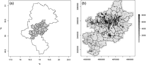
Fig. 1a shows the analysed area (grey) and the Silesian Voivodeship (white). Fig. 1b depicts the population density derived from [34], and the main heating arteries of the SHS system taken from the paper [27]. The infrastructure is located in the population hot-spot [16] what means the increasing number of dwellers increases the chances of the district heating infrastructure’s occurrence. This correlation between the population data results from the economic issues [35–37].

Figure 1. Location of the analysed area (grey) and the SHS’s arteries (black lines). a) In the Silesian Voivodeship. b) SHS arteries with the population density (inh./km²).

2.2. Linear Heat Density – literature review

Elaboration of the spatial emission inventories is frequently connected with the detailed spatial databases’ analysis using mathematical or statistical techniques [38–40]. Concerning available data sets, for elaboration of spatial emission inventories are highly usable e.g. land cover satellite imagery [5], spatial buildings’ classifications accordingly with their environmental properties [41–44], or population (density) data (as given in introduction).

The concept of the linear heat density (LHD), given in [35–37] can be also used to join the spatial information about the district heating arteries, with the population density data. Considering the problem of currently developed district heating systems Persson and Werner [35] clenched together the LHD with demographic quantities: (1) $$\text{LHD}≔\frac{Q_S}{L}\mathrm{}[\text{GJ}/\mathrm{m}]:=q·e·w,$$(1)

where: $Q_S$, total annually sold heat in a district heating system [GJ]; $L$, total length of the district heating piping network [m] $q$, annual specific heat demand: $$q\mathrm{}[\mathrm{J}/(\mathrm{m}2·\mathrm{a}\left)\right]:\mathrm{}=\frac{Q}{A_B}:$$

$Q$, heat delivered to buildings [J]; $A_B$, total building space area [m²]; $e$, city planning quantity plot ratio: $e\mathrm{}\left[\text{dimensionless}\right]:\mathrm{}=p·\alpha =\frac{P}{A_L}·\frac{A_B}{P}$:

$p$, population density in average dwelling [people/m²], $\alpha$, specific building space [m² per capita]; $P$, population [dimensionless], $A_L$, total land area [m²];

$w$, effective width $w:\mathrm{}=\frac{A_L}{L}\mathrm{}\left[\mathrm{m}\right]$.

The heat transferred by the pipelines is used for fulfilling the heating demand of the dwellers. Assuming constant heating demand per capita, the heat delivered to buildings (Q) is proportional to the population being supplied from the DHS.

2.3. Proportional spatial distribution of CO₂ emission

Official guidelines on spatial mapping of air pollutants’ emissions [19] consider the three methods of the residential emission’s (1A4bi) spatial disaggregation. The ’Tier’ classification presented below is in correspondence with the IPCC guidelines [20]. That means the air emissions’ spatial distributions elaborated accordingly to the consecutive ’Tiers’ are approaching to the unknown, actual spatial distribution of air emission. The classification and the correspondent spatial emission surrogate is presented below:

• Tier 1 – Land cover,

• Tier 2 – Population or household density combined with land cover data,

• Tier 3 – Detailed fuel deliveries for key fuels (e.g. gas) and modelled estimates for other fuels.

The ‘proportional’ spatial emission disaggregation is used frequently. The algorithm of the disaggregation assumes that the downscaled emission is proportional to the assumed emission allocator (surrogate), as below: (2) $${E_{{\text{CO}}_2}}_i\propto p_i,\mathrm{}\text{or}\mathrm{}{E_{{\text{CO}}_2}}_i\propto P_i,$$(2)

where for particular grid ‘i’ the downscaled CO₂ emission ${E_{{\text{CO}}_2}}_i$ [Mg] is weighted by the population density (p_i) or population data (P_i). Due to carrying out the emission’s spatial disaggregation in regular grid, the difference between the population and the population density is negligible. Population (density) is frequently used as a basic or auxiliary spatial emission surrogate, in larger spatial scales, such as global or regional.

2.4. Corrected spatial distribution of CO₂ emission

The correction introduced to the baseline, proportional spatial CO₂ emission distribution takes into account locations provided with the heat and hot water from the SHS heating system. These locations are determined using spatial classification function (mask) built from the information about the main district heating arteries’ spatial distribution given in the expertise [27] concerning the development of the SHS system. The spatial data is used directly. Similar data about spatial distribution of the district heating infrastructure can be also obtained from the local/regional geo-referenced datasets, municipal district heating network operators [43] or with introducing appropriate assumptions – from the heat demand maps [45]. The correction algorithm is elaborated in the language of statistical computing R [46–48], using the spatial intersection (∩) [49] for each grid cell i, as below: (3) $${\text{Mask}}_i=\left\{\begin{array}{c}0\mathrm{}\text{if}\mathrm{}HN\cap G_i=\mathrm{\varnothing }\\ G_i\mathrm{}\text{otherwise},\end{array}\right.$$(3)

where: $HN$, district heating network map (heating arteries, lines); $G$, gridded population density map, derived from [34], and aggregated to the 2 km ×2 km grid, as in Fig. 1(b); $HN\cap G_i=\mathrm{\varnothing }$ means that in the area of grid $G_i$, the length of heating network is equal to 0. Afterwards, in the first step, the Mask becomes corrected, as below: (4) $${\text{postMask}}_i=\mathrm{\kappa }·{\text{Mask}}_i,$$(4)

where $\mathrm{\kappa }$ is the contribution of inhabitants supplied with heat from the district heating system ($\mathrm{\kappa }=50\mathrm{\%},\text{see}2.1$). In the second – the population density grid G is covered by the mask [48]: (5) $$\text{postG}=\text{cover}\left(\text{post}\text{Mask},\mathrm{}G\right),$$(5)

(6) $${\mathit{\text{postG}}}_i=\left\{\begin{array}{c}{G}_i\mathrm{}\text{if}\mathrm{}{\text{postMask}}_i\cap G_i=\mathrm{\varnothing }\\ {\text{postMask}}_i\mathrm{}\text{otherwise}.\end{array}\right.$$(6)

Proposed methodology takes into account actual locations supplied with the heat and hot water, provided by the spatial distribution of the DHSs pipelines. Because for the different grid cells values of the population density are various, the reduced values also differ. DHSs pipelines are located mostly in highly populated grid cells.

3. Results and discussion

The Polish CO₂ emission data, 33,571.32kt from residential combustion (1A4bi), is derived from the UNFCCC repository [41] and corrected to the analysed area coverage using the population [42]. As the result, the analysed area emitted approximately 2,267.59kt of CO₂ (data for 2015). The same value is disaggregated using two approaches: ’proportional’ (section 3.1) and ’corrected’ (section 3.2).

3.1. Proportional spatial distribution of the residential CO₂ emission

The disaggregated CO₂ emission from the residential sector (1A4bi) is shown in the Fig. 2. The disaggregation (value) in each grid cell is proportional to the population density data. The emission peak values occurs directly in the area of the population hot-spot. The clearly visible spatial distribution of values exceeding 10 kt/year is arranged accordingly to the spatial distribution of the main arteries of the SHS system.

Figure 2. Residential CO₂ emission [kt/year] disaggregated in proportion to the population density.

The occurrence of the SHS’ main heating arteries in the area of the CO₂ mission hot-spot (see Fig. 1b) is a sign that using the population density as a spatial emission surrogate distinctly overestimates emission in locations supplied with the district heating systems. The table containing detailed statistics of the distribution is presented below (Table 1). The histogram of the disaggregated emissions is shown in the Fig. 3.

Figure 3. The histogram of the residential CO₂ emission [kt/year] disaggregated in proportion to the population density.

3.2. Corrected spatial distribution of the residential CO₂ emission

The corrected spatial distribution of the residential (1A4bi) CO₂ emission is elaborated using the κ value as a share of dwellers supplied with the heat and hot water from the SHS infrastructure. The algorithm subtracts the population density from the initial data (Fig. 1b) only inside these grid cells, which have non empty intersection with the SHSs’ infrastructure map (see lines in the Fig. 1b).

The subtracted value is proportional to the population density, and sum of subtracted values is equal to 50% of the analysed area’s population. The result is shown in the Fig. 4. The table with the distribution’s statistics and the histogram are presented below (Table 2, and Fig. 5, respectively).

Figure 4. Residential CO₂ emission [kt/year] disaggregated using correction applied to the population density.

Figure 5. The histogram of the residential CO₂ emission [kt/year] disaggregated using correction applied to the population density.

Figure 6. Population density derived from official statistics [inh./km²] vs. population density aggregated from grid [inh./km²].

3.3. Validation and remarks

According to the assumption (see 2.1), and the data provided in [27], the average share of dwellers supplied with the heat from the SHS system is 50%. The applied algorithm with population density correction, without optimization, estimated this share as nearly 53% (post-hoc analysis). It can be concluded, that the deviation from the actual data should not exceed 6%. The potential error of the applied algorithm is strictly connected with the quality of the used spatial data, however, considering the results obtained by Persson and Werner [35, 36], the algorithm of spatial disaggregation should take into account the district heating system. This remark can be treated as the indication, that the emission surrogates should be composed using the available spatial data.

In the second step we validated the data about population density. The population density aggregated in administrative units (see Fig. 1a) derived from the official statistics [29] is compared with the average population density aggregated from the 2 km ×2 km grid (see Fig. 1b). The result is presented in the figure below (Fig. 6).

Apart from comparison of population densities, we determined the ‘local $\mathrm{\kappa }$’ contributions which represent, as above, the share of population using district heating system, but for particular administrative units. For determination of the ‘local $\mathrm{\kappa }$’ we used aggregated data on population density before correction, and after that. The spatial distribution of the ‘local $\mathrm{\kappa }$’ for each administrative units is shown in the Fig. 7.

Figure 7. The spatial distribution of the ‘local $\mathrm{\kappa }$’ [dimensionless] – the share of inhabitants using the district heating system in particular administrative units.

In the next step we aggregated the ‘local $\mathrm{\kappa }$’s’ to the whole investigated area using the population data in particular administrative units derived from the official statistics [29]. The final aggregated value is nearly 49.6%, which is very close to the initial assumption (50%).

This result partly confirms conclusions of work [50] where it was investigated also population (density) in small and medium Japanese cities. That matter is also emphasized in [51] in the context of the influence of the infrastructure on the emission’s spatial distribution. The results presented in [52] stress the relationship between population density and (also) CO₂ emissions. Taking into account the area of the study (India), we can conclude indirectly that the CO₂ emission is going along with the population density, if the heating infrastructure does not occur in the analysed area.

The results obtained by the previously enumerated investigations suggest that the spatial distributions of the CO₂ emissions in the local scale should be corrected taking into account spatial distribution of the district heating arteries.

However the proposed algorithm uses actual spatial distributions of district heating arteries and population density, the result can be sensitive to further disaggregation (downscaling). It can be applicable in case of spatial analysis concerning urbanized agglomerations with buildings of homogenous age and thermal properties. For smaller areas, to describe strictly local impact of the small domestic combustion it will be better to apply approach ‘building by building’, given in [43, 44], however there is very limited possibility of direct comparison between various studies introducing more assumptions e.g. about the age of buildings. In that context, the goal considering the downscaling of the emission is achieved. Despite this shortcoming, presented way is very useful in case of limited access to geo-referenced data.

4. Conclusions

The study presented the algorithm for the spatial disaggregation of the CO₂ emissions from the residential (1A4bi) sector using spatial data about district heating infrastructure. However the spatial disaggregation along with the population (density) is acceptable for bigger scales (regional, global), for the local emission inventories should be corrected.

Proposed correction uses the spatial data about district heating infrastructure (map of the arteries) and decreases population density, when the district heating occurs. Correction is carried out using selected spatial techniques performed in statistical computing language R. Application of proposed algorithm distinctly changes the spatial distribution of the CO₂ emission in analysed area. However the study is presented for CO₂, the methodology will be associated with the analysis of CO₂ (GHGs) together with its precursors. Proposed methodology might be useful for the scientists, and also policymakers.

Table 1. Descriptive statistics of the spatial distribution of the residential CO₂ emission disaggregated in proportion to the population density [kt/year].

Min.	1^st Qu.	Median	3^rd Qu.	Max.	µ	σ
0.0000	0.1657	1.1416	3.789	25.5845	2.9373	4.334

Table 2. Descriptive statistics of the corrected spatial distribution of the residential CO₂ emission [kt/year].

Min.	1^st Qu.	Median	3^rd Qu.	Max.	µ	σ
0.0000	0.2822	1.3460	3.8209	40.1001	2.9373	4.4213

References

- M. Lesiv, R. Bun, N. Shpak, O. Danylo and P. Topylko, Spatial analysis of ghg emissions in eastern polish regions: energy production and residential sector, ECONTECHMOD, An International Quarterly Journal 1 (2012), pp. 17–23.
- K. Markakis, U. Im, A. Unal, D. Melas, O. Yenigun and S. Incecik, Compilation of a GIS based high spatially and temporally resolved emission inventory for the greater Istanbul area, Atmospheric Pollution Research 3 (2012), pp. 112–125.
- S.E. Puliafito, D.G. Allende, P.S. Castesana and M.F. Ruggeri, High-resolution atmospheric emission inventory of the argentine energy sector. Comparison with edgar global emission database, Heliyon 3 (2017), pp. e00489.
- T. Oda, S. Maksyutov and R.J. Andres, The Open-source Data Inventory for Anthropogenic CO2, version 2016 (ODIAC2016): a global monthly fossil fuel CO2 gridded emissions data product for tracer transport simulations and surface flux inversions, Earth System Science Data 10 (2018), pp. 87–107.
- H.P. Gibe and M.G. Cayetano, Spatial estimation of air PM2.5 emissions using activity data, local emission factors and land cover derived from satellite imagery, Atmos. Meas. Tech. 10 (2017), pp. 3313–3323.
- K.-M. Fameli and V.D. Assimakopoulos, The new open Flexible Emission Inventory for Greece and the Greater Athens Area (FEI-GREGAA): Account of pollutant sources and their importance from 2006 to 2012, Atmospheric Environment 137 (2016), pp. 17–37.
- V. Aleksandropoulou, K. Torseth and M. Lazaridis, Atmospheric Emission Inventory for Natural and Anthropogenic Sources and Spatial Emission Mapping for the Greater Athens Area, Water Air Soil Pollut 219 (2011), pp. 507–526.
- J. Maes, J. Vliegen, K. Van de Vel, S. Janssen, F. Deutsch, K. De Ridder et al., Spatial surrogates for the disaggregation of CORINAIR emission inventories, Atmospheric Environment 43 (2009), pp. 1246–1254.
- J. Ferreira, M. Guevara, J.M. Baldasano, O. Tchepel, M. Schaap, A.I. Miranda et al., A comparative analysis of two highly spatially resolved European atmospheric emission inventories, Atmospheric Environment 75 (2013), pp. 43–57.
- M. Trombetti, P. Thunis, B. Bessagnet, A. Clappier, F. Couvidat, M. Guevara et al., Spatial inter-comparison of Top-down emission inventories in European urban areas, Atmospheric Environment 173 (2018), pp. 142–156.
- D. van der Gon, H.A. C, J.J.P. Kuenen, G. Janssens-Maenhout, U. Döring, S. Jonkers et al., TNO_CAMS high resolution European emission inventory 2000–2014 for anthropogenic CO2 and future years following two different pathways, Earth System Science Data Discussions (2017), in review, pp. 1–30. doi: 10.5194/essd-2017-124.
- M. Kara, N. Mangir, A. Bayram and T. Elbir, A Spatially High Resolution and Activity Based Emissions Inventory for the Metropolitan Area of Istanbul, Turkey, Aerosol and Air Quality Research 14 (2014), pp. 10–20.
- R.J. Andres, T.A. Boden and D.M. Higdon, Gridded uncertainty in fossil fuel carbon dioxide emission maps, a CDIAC example, Atmospheric Chemistry and Physics 16 (2016), pp. 14979–14995.
- L. Ran, D.H. Loughlin, D. Yang, Z. Adelman, B.H. Baek and C.G. Nolte, ESP v2.0: enhanced method for exploring emission impacts of future scenarios in the United States – addressing spatial allocation, Geosci. Model Dev. 8 (2015), pp. 1775–1787.
- Z. Adelman, B. Naess, M. Omary and L. Ran, Recent Updates to Spatial Surrogates for Modeling U.S. Emissions Sources, 2015, pp. 19.
- D. Zasina and J. Zawadzki, Spatial surrogate for domestic combustion’s air emissions: A case study from Silesian Metropolis, Poland, Journal of the Air & Waste Management Association 67 (2017), pp. 1012–1019.
- H.C. Gils, J. Cofala, F. Wagner and W. Schöpp, GIS-based assessment of the district heating potential in the USA, Energy 58 (2013), pp. 318–329.
- S. Werner, International review of district heating and cooling, Energy 137 (2017), pp. 617–631.
- EEA, EMEP/EEA Air Pollutant Emission Inventory Guidebook 2016, 2016.
- IPCC Guidelines for National Greenhouse Gas Inventories. 2016, Available at https://www.ipcc-nggip.iges.or.jp/public/2006gl/.
- U. Leopold, G.B.M. Heuvelink, L. Drouet and D.S. Zachary, Modelling Spatial Uncertainties associated with Emission Disaggregation in an integrated Energy Air Quality Assessment Model, in: R. Seppelt, A.A. Voinov, S. Lange, D. Bankamp (Eds.), Proceedings of the 2012 International Congress on Environmental Modelling and Software, 2012, pp. 966–972.
- B. Zheng, Q. Zhang, D. Tong, C. Chen, C. Hong, M. Li et al., Resolution dependence of uncertainties in gridded emission inventories: a case study in Hebei, China, Atmospheric Chemistry and Physics 17 (2017), pp. 921–933.
- S. Hellsten, U. Dragosits, C.J. Place, A.J. Dore, Y.S. Tang and M.A. Sutton, Uncertainties and implications of applying aggregated data for spatial modelling of atmospheric ammonia emissions, Environmental Pollution 240 (2018), pp. 412–421.
- D. Ivanova, G. Vita, K. Steen-Olsen, K. Stadler, P.C. Melo, R. Wood et al., Mapping the carbon footprint of EU regions, Environ. Res. Lett. 12 (2017), pp. 054013.
- B. Białecka, Impact Assessment of the Upper Silesian Industrial Region on Greenhouse Gas Emissions in Poland, Water, Air, & Soil Pollution 148 (2003), pp. 335–346.
- J. Pełka-Gościniak, Threats and Values in the Area of Silesian Voivodeship, Acta Geographica Silesiana 17 (2014), pp. 79–83.
- M. Plebankiewicz and A. Jankowski, Cieplo dla aglomeracji miast slaskich do wsparcia z funduszy unijnych (Heat for the Silesian Agglomeration for support from the EU funds), Wokol energetyki 10 (2007), pp. 1–4.
- Statistics Poland, National Census of Population and Housing 2011, 2018. Available at https://stat.gov.pl/en/national-census/national-census-of-population-and-housing-2011/
- Statistics Poland, Local Data Bank. 2018. Available at https://bdl.stat.gov.pl/BDL/start.
- M.A. Sayegh, J. Danielewicz, T. Nannou, M. Miniewicz, P. Jadwiszczak, K. Piekarska et al., Trends of European research and development in district heating technologies, Renewable and Sustainable Energy Reviews 68 (2017), pp. 1183–1192.
- EUROHEAT, District Energy in Poland, Euroheat & Power, 2017. Available at https://www.euroheat.org/knowledge-centre/district-energy-poland/
- District Heating Market in Poland. 2017. Available at https://dbdh.dk/wp-content/uploads/District-heating-in-Poland-status-2017.pdf.
- Renewable Based District Heating in Europe - Policy Assessment of Selected Member States. Intelligent Energy - Europe, ALTENER, 2015.
- F.J. Gallego, A population density grid of the European Union, Popul Environ 31 (2010), pp. 460–473.
- U. Persson and S. Werner, Effective width – the relative demand for district heating pipe lengths in city areas, 2010.
- U. Persson and S. Werner, Heat distribution and the future competitiveness of district heating, Applied Energy 88 (2011), pp. 568–576.
- C. Reidhav and S. Werner, Profitability of sparse district heating, Applied Energy 85 (2008), pp. 867–877.
- O. Maimon and L. Rokach, eds., Data Mining and Knowledge Discovery Handbook, Springer US, New York, 2005.
- K.J. Cios, W. Pedrycz, R.W. Swiniarski and L. Kurgan, Data Mining: A Knowledge Discovery Approach, Springer US, New York, 2007.
- A. Taha, Knowledge Discovery In GIS Data, (2005), pp. 1–76. Master Thesis, Cairo University. Available at: https://arxiv.org/ftp/arxiv/papers/1601/1601.07241.pdf.
- G. Baiocchi, F. Creutzig, J. Minx and P.-P. Pichler, A spatial typology of human settlements and their CO2 emissions in England, Global Environmental Change 34 (2015), pp. 13–21.
- Y. Zhou and K. Gurney, A new methodology for quantifying on-site residential and commercial fossil fuel CO2 emissions at the building spatial scale and hourly time scale, Carbon Management 1 (2010), pp. 45–56.
- A. Wyrwa and Y. Chen, Mapping Urban Heat Demand with the Use of GIS-Based Tools, Energies 10 (2017), pp. 720.
- R. Cong, M. Saito, R. Hirata, A. Ito, S. Maksyutov and T. Oda, Anthropogenic carbon dioxide emissions in Tokyo metropolis estimated with a combination of top-down and bottom-up approach, 2017.
- Heat Roadmap Europe. 2018. Available at http://www.heatroadmap.eu/.
- R.S. Bivand, E. Pebesma and V. Gómez-Rubio, Applied Spatial Data Analysis with R, 2nd ed.Use R!Springer-Verlag, New York, 2013.
- R: The R Project for Statistical Computing, 2018. Available at https://www.r-project.org/.
- R.J. Hijmans, J. van Etten, J. Cheng, M. Mattiuzzi, M. Sumner, J.A. Greenberg et al., Raster: Geographic Data Analysis and Modeling, 2017.
- M. Ester, H.-P. Kriegel and J. Sander, Algorithms and Applications for Spatial Data Mining, 2001.
- Y. Makido, S. Dhakal and Y. Yamagata, Relationship between urban form and CO2 emissions: Evidence from fifty Japanese cities, Urban Climate 2 (2012), pp. 55–67.
- D. Timmons, N. Zirogiannis and M. Lutz, Location matters: Population density and carbon emissions from residential building energy use in the United States, Energy Research & Social Science 22 (2016), pp. 137–146.
- R. Ohlan, The impact of population density, energy consumption, economic growth and trade openness on CO2 emissions in India, Nat Hazards 79 (2015), pp. 1409–1428.