Introducing a new tool for greenhouse gas calculation tailored for cropland: rationale, operational framework and potential application

Abstract

The new GHG calculator named SECTOR (Source-selective and Emission-adjusted GHG CalculaTOR for Cropland) is based on the IPCC Tier 2 approach for rice as well as other crops. The new features of SECTOR facilitate high flexibility in terms of entering newly obtained emission factors, easy data transfer from crop statistics for entering activity data and detailed specifications of GHG scenarios. A new procedure of entering frequency-based data on current water management practices was also developed. Moreover, the tool allows deviating from the 2006 IPCC Guidelines by considering field records with high background levels of N₂O emissions in the overall assessment of GHG emissions.

This article assesses different applications of the tool, namely as add-ons to field measurements, for GHG calculation at national/sectorial scale and within measurement, reporting and verification of development projects. SECTOR is downloadable in the form of templates that can be used to develop custom versions with varying levels of disaggregated data entries at different scales. A case study for rice production in one Vietnamese province demonstrates the potential to display GHG results in combination with GIS. SECTOR can easily be adjusted to incorporate new emission factors and calculation procedures expected in forthcoming revisions of the IPCC Guidelines.

Highlights

• A new GHG calculation tool was developed based on the IPCC Tier 2 approach for rice as well as other crops

• Features of the tool facilitate high flexibility in terms of emission factors, easy data transfer from crop statistics for entering activity data and detailed specification of GHG scenarios

• This article assesses different user groups and possible applications of the tool

• A case study for rice production in one Vietnamese province demonstrates the potential to display GHG results in combination with GIS

Keywords:

• GHG calculation tool
• Tier 2
• emission factors
• activity data
• Thai Binh Province (Vietnam)

Introduction

When initial field data on CH₄ emissions from rice fields became available in the 1980s and 1990s, this almost immediately led to an extrapolation of the emission rates to global scale [e.g. 1–3]. However, these estimated source strengths were obtained by simple multiplication of the emission rates recorded in field experiments with the global rice area. As a response to the reporting commitments under the United Nations Framework Convention on Climate Change (UNFCCC), the Intergovernmental Panel on Climate Change (IPCC) was commissioned to develop guidelines for national GHG inventories. These guidelines have been used worldwide by most countries for their National Communications to the UNFCCC. Following this, national GHG inventories were compiled at global scale in GHG databases by the Emissions Database for Global Atmospheric Research (EDGAR, http://edgar.jrc.ec.europa.eu/) so that the shares of individual sectors could be quantified globally. In a parallel development, Food and Agriculture Organization Corporate Statistical Database (FAOSTAT) compiled emission estimates based on agricultural statistics that can be specified for given years in the past as well as for future scenarios (http://www.fao.org/faostat/en/#data/EM). As a consequence of the recent GHG inventories, it became a widely accepted estimate that 15% of the global GHG emissions are attributed to agriculture which includes a share of 1.5% for rice alone [1].

In the initial round of National Communications to the UNFCCC, few rice growing countries had field data available to come up with country-specific emission factors (EFs). With the exception of China and India, all rice-growing countries in Asia have used the Tier 1 approach in the GHG inventory within the initial National Communications. This picture has changed since the 2^nd National Communications where many rice-growing countries now use the Tier 2 approach with newly obtained country-specific EFs. While those initial field experiments as well as national programs have mainly been based on the ‘closed chamber method’ with manual sampling, a wide range of advanced approaches with different measurement and monitoring techniques has now been developed for direct or indirect assessment of GHG emissions from agriculture across different scales [4,5].

The rapidly growing interest in GHG assessments observed in recent years can to a large extent be attributed to the Paris Agreement of 2015 in which the UNFCCC parties commonly agreed on limiting global warming by 1.5 to 2 °C above pre-industrial levels. To communicate their Nationally Determined Contributions (NDCs) in mitigation reduction, all parties are requested to publish their post-2020 intended climate actions. This international agreement enables the parties to get an overview about all planned and conducted actions and will help to determine whether the common efforts are sufficient to reach the overall agreed goal of temperature reduction. UNFCCC has also introduced Nationally Appropriate Mitigation Actions (NAMAs) that can be seen as an operational strategy toward achieving the long-term goals of NDCs, and can contribute to preparation for country-specific NDCs [6].

While the importance of adaptation in the agriculture sector has never been in question, its potential role in mitigation has recently also been recognized in official documents. COP 17 (2011) initiated a process that led to establishing the UNFCCC Koronivia Joint Work on Agriculture in 2017. The aim of this UNFCCC initiative is to develop and implement new strategies for the agriculture sector including the reduction of emissions [7]. This initiative stresses the need for both adaptation and mitigation strategies as well as possible co-benefits between them.

GHG emissions from rice have been investigated in many field studies, but this wealth of information is hardly used for GHG calculations at larger scales. Due to the predominant flooding of rice soils this production system also offers specific mitigation options based on modified water regimes, namely alternate wetting and drying (AWD) [8], which corresponds to ‘Intermittently flooded – multiple aeration’ in the IPCC terminology. Subsequently, rice and AWD are mentioned in many NDCs of Asian countries [9].

In turn, there is an urgent need to develop measurement, reporting and verification (MRV) systems for rice production that can provide ex-ante assessments in proposals as well as ex-post assessments for documenting project impacts. GHG assessments for rice are typically based on the IPCC guidelines that can be applied in various forms including with the use of GHG calculators. Whereas the IPCC guidelines were developed for the purpose of GHG inventory at the country scale, they have in the meantime been used at the scale of individual projects. In the case of rice production, this application at project scale has also been incorporated into the UNFCCC-approved methodology titled ‘AMS-III.AU’(https://cdm.unfccc.int/methodologies/documentation/meth_booklet.pdf# AMS_III_AU). However, this UNFCCC methodology for Clean Development Mechanism (CDM) projects is not very prescriptive in terms of the monitoring approach and leaves different options for the potential user that are discussed in this article.

Review of GHG calculation tools

In a comprehensive review in 2013 [10], a total number of 18 GHG calculators were identified for the agriculture sectors, amongst them EX-ACT [11], Cool Farm Tool [12] and ALU [13]. This list of GHG calculators has expanded since then by the release of new tools for specific purposes, such as MOT [14] targeting mitigation assessments, and GLEAM [15] focussing on livestock emissions. GHG calculation has also been included in broader assessments of environmental impacts and sustainability, for example the Field Calculator of the Sustainable Rice Platform [16].

All these calculators – as well as the new tool called Source-selective and Emission-adjusted GHG CalculaTOR for Cropland (SECTOR) – are based on the IPCC approach. Thus, it is unavoidable that those tools will show similarities in their structure and actual use while they differ in some individual features, such as:

• Overall purpose (inventory, mitigation assessment or both);

• Geographic domain (ranging from farm scale to national area);

• Scope of activity data;

• Inclusion of off-farm emissions;

• Skills required for operations.

Some of the tools strictly adhere to the IPCC formulas (e.g. ALU [13]), due to the intended use within national GHG inventories, while other tools expand these formulas to include off-farm emission sources (e.g. EX-ACT [11]). In this regard, SECTOR can be seen as a multi-purpose tool that allows a high degree of flexibility for IPCC calculations to be accomplished with or without considering other GHG sources (see below).

The development of these calculators has been driven by the desire to provide a readily available tool for users – especially those who may not have high familiarity with the IPCC approach. As a consequence, these calculators have been used in very diverse contexts, such as providing information within a policy debate [17], decision-making on future development [18] and project proposals (e.g. http://www.nama-facility.org/projects/thai-rice-nama).

Moreover, such tools have also been applied for generating product/market-oriented information and are often related to C footprint assessments that are in turn often related to specific commodities [19,20]. Emissions at the production stage cover only one part of the C footprint of an agricultural product, but in the case of rice (and dairy products) the field emissions make up the bulk of the C footprint [21]. Thus, the GHG calculators provide essential information for C footprint analysis of these products. It seems likely that several of these GHG calculators will eventually evolve into more comprehensive assessments of the entire value chain, as can be seen already in the most recent development of EX-ACT (http://www.fao.org/tc/exact/ex-act-tool-for-value-chains/en/).

Basic concept and new features of SECTOR

Within the course of working in mitigation projects, it became increasingly clear that such projects require a number of additional software features that are not available in existing GHG calculation tools. Thus, a new tool was developed that has been named SECTOR (Source-selective and Emission-adjusted GHG CalculaTOR), based on the IPCC 2006 Guidelines [22], which incorporates several features for improving performance within mitigation projects (Table 1). This tool is available as an XLS file and can be downloaded from http://climatechange.irri.org/SECTOR. The software also comes with a detailed User Manual [23] and a Demo File; therefore, this article’s content is limited to outlining the basic and innovative features of SECTOR software.

Table 1. Overview of specific Tier 2 requirements for GHG calculations in cropland within mitigation projects and approach in SECTOR.

Specific requirement		Approach implemented in SECTOR
Emission factors (EFs)	Free choice of EFs from IPCC and other sources	Emission library that can easily be expanded by location-specific EFs
Activity data	Rapid transfer of activity data from statistics or survey data for large number of patches	Entry format allows ‘copy-paste’ of area, yield and fertilizer data for up to 100 patches
	Entry of activity data with frequencies (percentages) of water management practices	See new procedure described in “New procedure for entering frequencies of different BAU water management practices”
Aggregation	Aggregation for multiple seasons and scenarios	Aggregation framework with triangulation of GHG data (patch/season/scenario)
Scenario setting	Accounting for efficiencies in adoption of mitigation options	New coefficients for fertilizer-use efficiency as well as biophysical and economic barriers to adopting mitigation options

Emission factors

In the context of ‘disaggregation’ within the IPCC guidelines, the aim is that data from field measurements should preferably be utilized – in a transparent manner – for GHG calculations in the respective domain. On the other hand, IPCC values should still be included in the calculations as a benchmark to ensure consistency with results from other studies. Ideally, GHG calculators should contain a library of EFs comprising IPCC values that can be easily extended with data from other sources. Thus, the user should have free choice in using experimental results as EFs, so that GHG calculations using their own data source can be juxtaposed with results based on IPCC values.

Activity data

The input procedures of available GHG calculators require manual entry which becomes a cumbersome and time-consuming step in the case where numerous entities are considered. On the other hand, rice statistics typically provide data on areas and yields (and in some cases also fertilizer rates), so the aim should be to utilize this data at the smallest administrative scale available. Likewise, the data from farm surveys will in most cases result in larger tables of activity data for each farm. Thus, the GHG calculators should allow batch transfer (copy-pasting) of tabulated data. This input procedure is especially important if the number of patches (farms, provinces, etc.) is large.

The GHG calculations in the IPCC equations basically assume one value for a given crop management practice for a given area. In typical farm surveys, however, information coming from a large number of farmers results in percentages of individual management practices that cannot at present be entered into existing GHG calculators; for example, for water management this may result in 50% of the farmers applying the IPCC category ‘Continuous Flooding’ (CF), 30% ‘Intermittently flooded – single aeration’, and 20% ‘Intermittently flooded – multiple aeration’. For rice production, water management is the key factor for determining business-as-usual (BAU) emissions – and thus for assessing mitigation potentials. Therefore, a new input procedure was developed for entering frequency-based information on BAU of water management (see "Input procedures and outputs/ STEP II: Enter project and statistics data").

Spatial and seasonal aggregation

Given the heterogeneity of crop production, mitigation projects targeting larger domains should disaggregate the total area into smaller spatial units. Conceptually, the aggregation framework for cropland can be presented by distinct patches constituting one spatial domain (Figure 1a). These patches can be distributed within the domain in a fragmented pattern (as shown in Figure 1a) or forming a coherent area – that is, corresponding to tiles that are adjacent to each other. Depending on the project context, GHG aggregation has to be done at a range of different scales, such as several farms being aggregated to one village, several villages to one district, etc. (Figure 1b).

Figure 1. (a) Schematic overview of spatial aggregation from patches to domain; (b) possible patch-domain pairs at different scales.

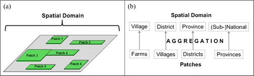
For aggregation at larger scale (e.g. provinces to the whole country), data on crop management may be derived from surveys conducted with a representative set of farmers using application rates of synthetic and organic fertilizers within one patch.

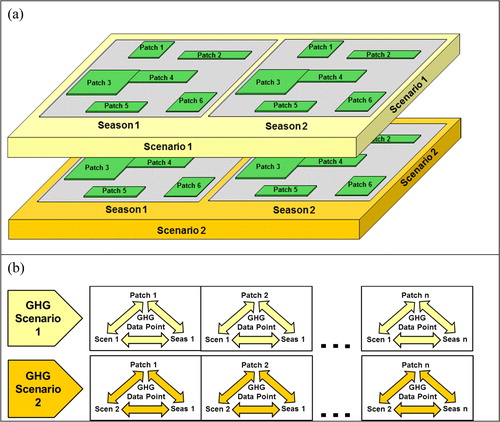
This spatial structure of patches within one spatial domain is expanded by adding seasons and scenarios (Figure 2a). Thus, the individual data points for GHG assessments are triangulated by patch, season and scenario (Figure 2b). Most rice production systems have two cropping seasons per year, but the maximum number should be three seasons as found in some highly intensive rice systems. It is assumed that Scenario 1 will in most applications be BAU and the other scenarios will correspond to mitigation. Users may want to assess three scenarios at the same time, which will allow them to study the impact of two mitigation scenarios versus BAU (see "New procedure for entering frequencies of different BAU water management practices").

Figure 2. (a) Schematic overview of patches, seasons and scenarios; (b) triangulation of GHG data points.

Specifications for scenario settings

Under the IPCC methodology, scenarios can be set and compared by setting different EF and SF (scaling factor) values for example SF_w for water management (Table 2). For increased efficiencies of fertilizer N, however, this procedure cannot be accomplished by EF or SF adjustment alone, because the quantity of N is used in several equations in the IPCC methodology for on-site and off-site GHG emissions. Thus, a new coefficient was introduced to account for N-use efficiency in SECTOR. For instance, if an improved practice of fertilizer application (e.g. site-specific nutrient management) can reduce the N requirement by a factor of 20%, then this coefficient can be set to 0.8 which will adjust the figures for N amounts in all IPCC Tier 2 equations requiring this input data.

Moreover, any conceivable mitigation project in the agriculture sector will have to cope with bio-physical and economic barriers to adopting mitigation options. Thus, it should be possible for the users to specify such barriers for a given technology for individual patches, seasons and scenarios. This specificity is especially important for determining barriers in adopting water management practices, namely AWD. Seasons with heavy rainfall will impede AWD in some locations and generally reduce the incentive for farmers to save water.

Conceptually, such barriers can be expressed through coefficients on a scale from 1 to 0 in which ‘1’ stands for no constraints and ‘0’ indicates the impracticality of the mitigation option. Consideration of topographic and climatic constraints of management practices could be determined by a bio-physical coefficient (BC). Likewise, an economic coefficient (EC) could be introduced to account for different degrees of incentives for farmers.

New procedure for entering frequencies of different BAU water management practices

Given the significance of water management for GHG emissions in rice, a new procedure was developed of entering BAU data in the form of percentages of farmers who apply distinct practices, as opposed to assuming one uniform practice within a given patch. The procedure for entering frequency-based information on BAU activity data is based on the proportional change of the SF value for a given patch/season. The newly introduced parameter ‘frequency-weighted SF-values’ (øSF) is illustrated in Table 2 and described below for the case of SF_w. It should be noted, though, that frequency data on SF_p can be handled in a similar fashion.

Table 2. Example for frequency (percentage) survey data for different SF_w values and frequency-weighted SF_w value for entire GHG data point (patch/season/scenario).

Water management	IPCC value	Frequency in survey	øSFw
Continuous flooding	1	0.2	0.64 (= 1* 0.2 + 0.6* 0.3 + 0.52 * 0.5)
Single aeration	0.6	0.3
Multiple aeration	0.52	0.5

Equation 1. Combined from two equations in IPCC 2006 (IPCC Equation 5.1 and 5.2 by assuming all other SF values equal 1): $${\text{CH}}_{4\text{Rice}}={\text{EF}}_{\mathrm{c}}·\mathrm{t}·\mathrm{A}·{\text{SF}}_{\mathrm{w}}$$

In which

CH_{4 Rice} = annual methane emissions from rice cultivation, kg CH₄ yr⁻¹

EF_c = baseline emission factor for continuously flooded fields without organic amendments, kg CH₄ ha⁻¹day⁻¹

t = cultivation period of rice, day

A = annual harvested area of rice, ha

SF_w = scaling factor for water regime

This equation only allows one value for SF_w as well as one value for the area. In terms of area, these frequencies correspond to three sub-areas expressed by the total area multiplied by the frequencies of each water management:

Equation 2: $${\text{CH}}_{4\text{Rice}}={(\mathrm{E}\mathrm{F}}_{\mathrm{c}}·\mathrm{t}·{10}^{-6}·\mathrm{A}·{\mathrm{F}}_{\mathrm{c}}·{\text{SF}}_{\text{w}\_\mathrm{c}})+({\text{EF}}_{\mathrm{c}}·\mathrm{t}·{10}^{-6}·\mathrm{A}·{\mathrm{F}}_{\mathrm{s}}·{\text{SF}}_{\text{w}\_\mathrm{s}})+({\text{EF}}_{\mathrm{c}}·\mathrm{t}·{10}^{-6}·\mathrm{A}·{\mathrm{F}}_{\mathrm{m}}·{\text{SF}}_{\text{w}\_\mathrm{m}})$$

In which

F_c,s,m = frequency of continuous flooding (c), single aeration (s) and multiple aeration (m), respectively, as derived from survey data SF_{w_c,s,m} = scaling factor of continuous flooding (c), single aeration (s) and multiple aeration (m), respectively (from [22])

In the next step, this equation can be simplified as follows:

Equation 3: $${\text{CH}}_{4\text{Rice}}={\text{EF}}_{\mathrm{c}}·\mathrm{t}·{10}^{-6}·\mathrm{A}·\left({\mathrm{F}}_{\mathrm{c}}·{\text{SF}}_{\text{w}\_\mathrm{c}}+{\mathrm{F}}_{\mathrm{s}}·{\text{SF}}_{\text{w}\_\mathrm{s}}+{\mathrm{F}}_{\mathrm{M}}·{\text{SF}}_{\text{w}\_\mathrm{m}}\right)$$

$$={\text{EF}}_{\mathrm{c}}·\mathrm{t}·{10}^{-6}·\mathrm{A}·{ø\text{SF}}_{\mathrm{w}}$$

The term øSF_w denotes the weighted SF value that can be computed for the entire area as shown in Table 2. This will need simple pre-processing of the survey data before entering these values into the GHG calculation.

Input procedures and outputs

All files needed for the GHG calculations are placed in the folder ‘SECTOR’. The folder includes the XLS file and the manual, as well as a file named ‘Demo.XLS’ which presents an example of a completely filled SECTOR file. The SECTOR templates as well as the demo file contain nine worksheets that are described in detail in the manual. The data input procedures are done in five steps as shown in the flow chart (Figure 3).

Figure 3. Flowchart of operations in SECTOR.

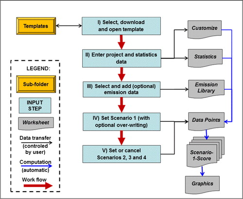
STEP I: Select, download and open template

One of the new features of SECTOR is that the user can choose among a set of templates according to the number of seasons (max. 3) and patches (max. 100). This selection procedure has been introduced for convenient use of the resulting files and their outputs by the user. The principal calculations, however, are identical in all templates, so as such there will be impacts on the results.

STEP II: Enter project and statistics data

The operation of the SECTOR tool is done in ‘projects’, so the user has to start by defining a project name. Then, data on areas, yields and fertilizer use can either be entered manually or be transferred by copy-paste from another file (e.g. statistics). In a preceding step, however, the respective statistics data may have to be formatted, for example by transposing of data lines as described in the Manual. SECTOR also allows adjusting the water management practice (BAU), for example accounting for 50% CF, 30% single aeration and 20% multiple aeration, as explained in the Manual.

STEP III: Select and add (optional) emission data

SECTOR includes an ‘Emission Library’ which contains the IPCC values for global warming potential (GWP), EF and SF. These values will be shown in drop-down menus during operations. These data lists can easily be expanded by additional EF and SF entries into the library (e.g. entering site-specific Tier 2 data).

STEP IV: Set scenario 1 (with optional overwriting)

The worksheet ‘Data Points’ displays all inputs and default values or the GHG calculations that are automatically adopted from the other worksheets as ‘scenario-wide’ values. These values are automatically copied for all patches and seasons of a given scenario, as shown in Figure 4a.

Figure 4. Operations in the ‘Data Points’ worksheet for an example with two seasons and two scenarios: (a) scenario-wide and data-specific entries (over-writing); and (b) setting and cancelling of scenarios.

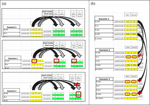
However, SECTOR also offers the option to specify individual data points independent of the scenario-wide settings. To some extent this is already built into the ‘Statistics’ worksheet, because these data on area and yields are used in the SECTOR calculations of the output worksheets. In the ‘Data Points’ worksheet, the user can overwrite the given scenario-wide value by entering a point-specific value in the green cell under the respective value (Figure 4a).

The GHG computation for upland crops will only require setting ‘EF_CH₄’ to the value ‘0’ and ‘EF_N₂O to ‘0.01’, so that methane emissions are assumed to be non-existing and nitrous oxide emissions are set according to the IPCC default value for upland crops. It is understood that the IPCC value for EF_N₂O (1% of all N fertilizer applied) can also be replaced by another value that has been entered into the ‘Emission Library’ worksheet.

STEP V: Set or cancel scenarios 2, 3 and 4

The ‘Data Points’ worksheet also comprises the settings for scenarios 2, 3 and 4. Figure 4b shows the procedure for specifying scenario settings, which is illustrated for different water managements. This can easily be accomplished by replacing the original SF_w value of ‘1’ (=continuous flooding) with ‘0.52’ (=multiple aeration). Triggered by the procedure explained above, these values will now be adopted for all patches and seasons within the respective scenario, while individual values can still be overwritten. The required data entries for two alternative scenarios also allow additional entries for ‘Fert N saving ratio’ to account for improved fertilizer management as a mitigation strategy. Moreover, SECTOR introduces two coefficients to express barriers to implementing mitigation options, namely the BC and the EC. Those coefficients can be set by the user as a means to realistically assess the chances of implementing a given mitigation technology.

All input data are automatically used for the computations in the score worksheets. Emissions are given for each patch and season as well as aggregated for the entire domain and displayed as diagrams.

Demonstration for Thai Binh province (Vietnam)

To illustrate the potential use of SECTOR, activity data were compiled for one example at the province scale. Thai Binh was chosen, which is the major rice-growing province in the Red River Delta of Vietnam, and activity data at the district level (M.V. Trinh and V.D. Quynh, Unpublished Data) were used, namely area, season length and N fertilizer rates for the spring season (Spr_) and the summer season (Sum_). Then, four emission scenarios were compiled using different EFs for CH₄ and N₂O as shown in Table 3. In addition to the IPCC default value (for CF) empirical data were used for the Red River Delta, that were obtained through field experiments [24] conducted over two continuous rice-growing seasons under CF as well as – using the IPCC terminology – single aeration (1xAe) and double aeration (2xAe).

Table 3. Activity data and emission factors in spring (Spr) and summer (Sum) rice seasons in Thai Binh province; emission factors for CH₄ (EF_CH₄) and N₂O (EF_N₂O) comprise IPCC default values for continuous flooding (CF) and empirical data (shaded in gray) for the Red River Delta from Tariq et al. [24] for CF, single aeration (1xAe) and double aeration (2xAe).

	Cumulative CH4 emissions (kg/ha)	EF_CH4 (kg/ha/d)	Cumulative N2O emissions (kg/ha)	EF_N2O (%)
Spring season* (total area: 78,590 ha; avg. season length: 100 d; avg. N fert.: 106.7 kg/ha)
Spr_IPCC		1.3		0.3
Spr_CF	129.6	1.296	129.6	1.296
Spr_1xAe	92.1	0.921	92.1	0.921
Spr_2xAe	36.1	0.361	36.1	0.361
Summer season* (total area: 79,500 ha; avg. season length: 85 d; avg. N fert.: 104.6 kg/ha)
Sum_IPCC		1.3		0.3
Sum_CF	698.5	8.218	0.3	0.22
Sum_1xAe	485.5	5.712	0.1	0.07
Sum_2xAe	222.6	2.619	0.7	0.51

*Activity data at the district scale was entered into SECTOR.

Activity data and EFs were entered into SECTOR following the procedures described in the SECTOR Manual [23]. These four EFs per season were treated as distinct scenarios to compute the resulting emissions at district scale. Then, these results were mapped using open-source GIS software (QGIS) that can be downloaded jointly with detailed tutorials under https://qgis.org. The initial step for this mapping procedure was to save the results of each season/scenario as a CSV file to allow joining of the emission data to a shape file downloaded from https://gadm.org/maps/VNM/thaibinh_2.html.

The results of these GHG calculations are shown in Figures 5 and 6, displaying one chloropleth map per season and scenario. As can be seen in Table 3, emission rates were fairly low in the spring season and substantially higher (by about a factor of 5) in the summer season, which is also reflected in these maps. Due to the different magnitudes in GHG emissions, distinct color classifications were defined for the chloropleth map of each season, namely seven classes ranging from 0 to 63 kt CO₂e/Season and 0 to 360 kt CO₂e/Season, respectively (see legends of Figures 5 and 6).

Figure 5. GHG emissions in Thai Binh Province from rice in the spring season calculated using different emission factors, namely the IPCC default value and empirical data from Tariq et al. [24] for continuous flooding (CF), single aeration (1xAe) and double aeration (2xAe).

Figure 6. GHG emissions in Thai Binh Province from rice in the summer season calculated using different emission factors, namely the IPCC default value and empirical data from Tariq et al. [24] for continuous flooding (CF), single aeration (1xAe) and double aeration (2xAe).

The basic idea behind the type of illustration shown in Figures 5 and 6 is to identify emission and mitigation potentials over space and time. The IPCC default map can be taken as a benchmark for this purpose. In the present example, the IPCC default map looks spatially differentiated for the spring season while all districts fall within the lowest two classes of GHG emissions for the summer season. Derived from these maps, it could easily be concluded that the most efficient strategy to achieve high mitigation impacts is to focus on information campaigns to promote AWD adoption by farmers in the summer season and, more specifically, to target the Central/Eastern districts of the province. It is understood, however, that the actual way to evaluate and display the results from SECTOR will largely depend on the overall objective of the user (see below). This simple example should nevertheless provide an idea of the possible use of the GHG calculations within the aggregation framework and tool described in this article.

Discussion

Potential SECTOR user groups

SECTOR comes with a number of features that will allow a high degree of flexibility and efficiency in incorporating data from different sources. While a simple demonstration is provided for using SECTOR, the authors recognize that there may be very different approaches to displaying and using GHG emission data depending on the rationale for the GHG calculation and the specific interest of the users. While this tool was developed in the context of mitigation studies conducted at the International Rice Research Institute (IRRI), it could be instrumental for a broader audience that can be broken up into three main user groups in terms of their respective context of application:

• Researchers engaged in field measurements of GHG emissions with the intent of using newly acquired EFs for extrapolation to larger domains (e.g. subnational regions). This group can be exemplified by the Greenhouse Gas Mitigation in Irrigated Rice Systems in Asia (Part 2) known as MIRSA-2 project that has conducted field measurements with harmonized measurement protocols and Quality Assurance/ Quality Control procedures in Thailand, Vietnam, the Philippines and Indonesia [25]. While this new data set is now documented in four country-specific publications and one cross-cutting publication, it seems unclear how it can actually be used to improve GHG estimates in the region – as long as a clear framework for the data integration is lacking.

• Projects on agricultural development and – as a new project category – GHG mitigation requiring GHG impact assessments under different scenarios of technology adoption. With the parallel assessment of BAU and mitigation scenario, SECTOR could become a convenient tool for ex-ante and ex-post evaluation of mitigation projects. The software can therefore be incorporated into the monitoring and evaluation system of such projects. A rigorous but quick assessment of the mitigation benefit of project activities will ease the planning process and make it easy to evaluate its impact.

• Institutions involved in GHG calculation at the national/sectorial scale, namely National Communications, NAMA and NDC.

Given the growing interest in GHG data, it can be expected that many countries will intensify their efforts over the coming years to meet their reporting commitments and reach defined mitigation targets over the next few years. With the decisions reached at COP 23 in 2018, the agriculture sector will play a larger role in mitigation planning [26]. This will also affect rice production, which is a key source of emissions in many Asian countries. SECTOR represents a convenient tool to keep track of various mitigation activities in different regions, to aggregate the results and to evaluate their effectiveness. As such, the tool can then be used to plan further mitigation activities or to adjust ongoing ones. The prospects for such activities are discussed below in relation to the policy environment.

Integration of SECTOR within an MRV framework for agriculture

Although the acronym MRV is semantically ambiguous,¹ there is broad consensus that MRV is needed to track the efficiency of mitigation options and to ensure transparency and credibility of results [27,28]. However, the bulk of the literature dealing with MRV issues addresses its role at the national level for planning and implementing NDCs. MRV frameworks at project scale have only vaguely been defined at present.

The new features of SECTOR address some of the major challenges for developing sound concepts for an agricultural MRV framework. For instance, the diversity of crop management practices makes it difficult to account for them in the other calculation tools that assume one uniform practice in a given area. Given the significance of water regimes for overall emissions, mitigation projects will have to establish a solid baseline by recording the frequency of farmers following a certain practice that can then be compared to the situation at the end of the project.

The reliability of IPCC default values for point sources in agriculture (including rice fields) has recently been questioned [29]. At the national level, the rationale for using one global default value is that local deviations in terms of very high or low emission rates will somehow level off at the national scale. As such, it is not really surprising that locally obtained emission rates deviate from the national – or global – default values used in any given GHG calculator. But this disparity between local and default EFs does not necessarily speak against using the IPCC approach as such, and only corroborates the need for disaggregation of EFs to be integrated into the GHG calculation. Since the wealth of empirical records on emissions has not really been tapped for GHG calculations in the past, it is hoped that the new GHG calculation tool with user-friendly inputs of local data may stimulate a broader use and sharing of GHG data.

Potential adjustments for new findings on background levels of N₂O emissions

The IPCC 2006 Guidelines treat N₂O emissions in a fairly simplistic way, namely by assuming 1% of all fertilizer N is emitted as N₂O in upland crops and 0.3% in flooded rice. While this approach was derived from the available data in 2006 [30], there is a growing body of evidence that these uniform ratios often deviate from empirically determined emissions. Several meta-analyses published over recent years reveal a large variation in background levels of N₂O emission rates from different sites [31–33]. Moreover, the impact of different water management practices on N₂O emissions from rice will deserve more consideration in light of newly published experimental data [34]. High N₂O emissions as reported in this publication cannot be covered by the IPCC approach based on N fertilizer rates, and thus will require a new input procedure to be incorporated into GHG calculations. Irrespective of the ongoing debate on the significance of these new findings with extremely high N₂O emissions, a new parameter is included to account for such high background levels of N₂O emissions, called the singular N₂O emission factor (‘singN₂O_EF’). While the respective cells in the ‘Emission Library’ worksheet are still empty, it will be easy for a user to enter new data on N₂O emissions that will be directly added to the overall emissions. Once the data has been entered in the ‘Emission Library’ worksheet, it can then be selected in the ‘Data Points’ worksheet just like any other EF. The scenario-based structure of SECTOR will also allow a specific combination of background EFs for N₂O and a given water management type (e.g. setting SFw = 1 for continuous flooding in Scenario 1 and SFw = 0.52 for multiple aeration in Scenario 2). Thus, the user will have the option to either to adhere to the IPCC algorithm for N₂O emissions or incorporate individually obtained N₂O emission rates into the overall calculation procedure.

Conclusion

Several research groups have conducted field experiments to determine emission rates in rice and other crops. But what is actually done with all this wealth of data? The actual use of these data sources for the purpose of GHG assessments seems to be very limited. Apparently, there is a disconnect between the different groups of researchers, namely those doing field measurements and those dealing with regional estimates.

We assume that this disconnect can to a large extent can be attributed to the methodological problems in integrating newly generated field data into GHG assessments for larger domains. As such, we are confident that the generic aggregation framework presented in this paper as well as the new GHG calculation tool may become instrumental in producing more flexible and reliable GHG assessments. While the framework and tools are so far only applicable to rice, it requires only an incremental step to expand this to other crops as well.

GHG calculators have been the method of choice for the vast majority of applications that require GHG assessments – and it seems almost certain that this will remain the case for the time being. The advantages from a user’s perspective are clearly their simplicity in operations and fairly low requirements in terms of data inputs. These advantages are evident irrespective of the software language that could be Excel, an online tool or a mobile phone app.

Moreover, all available GHG calculators have a common methodological framework, namely the IPCC approach. As this is recognized as the official approach for GHG inventories, the use of such calculators also comes – rightly or wrongly – with a certain credibility as a reliable tool. This perception of scale-transient GHG calculation has also been endorsed by the official UNFCCC methodology that adopted the basic principles of the IPCC approach for CDM projects in rice production.

Simulation models could at least potentially become a more reliable alternative in the future. These models have been shown to be very valuable research tools for GHG emissions from crops in general and in rice production particularly, such as new models developed from DeNitrification DeComposition (DNDC) [35,36]. By the nature of these simulation models, however, their application has to undergo an on-site validation (including GHG measurements) and will require considerable skills [37]. However, it seems unrealistic at this point to expect their widespread application by different user groups in the near future.

The use of the IPCC approach for scales other than initially intended seems justifiable as long as an appropriate EF is chosen. Moreover, the number of EFs can be expanded in the case of site-specific settings, such as adverse soils. However, the 2006 IPCC Guidelines do not consider any site-specific variations of SF_w, SF_p or SF_o in the method for calculating methane emissions from rice. This lack of flexibility can be attributed to the scarcity of empirical data on different crop management treatments at the time of writing the guidelines. At this point, however, effectively all measurements in rice production are conducted with parallel assessments of CF versus AWD. Thus, it seems incomprehensible that this kind of direct comparison should be discarded for one global SF. We have therefore developed the new tool with a provision for directly determined SF_w, SF_p and SF_o values while the principle of assigning one EF for baseline treatment (continuous flooding; no organic amendments) will be maintained.

For mitigation projects, we feel that the consideration of bio-physical and economic efficiencies should be seen as imperative in rice as well as other agricultural systems. At this point, there is no universally applicable methodology for assessing these coefficients, but GIS studies on AWD suitability may point in the direction of a more profound assessment of these constraints in the future [38,39].

Even though the current version of SECTOR is based on the 2006 IPCC Guidelines, the principal improvements embedded in the tool (Table 1) will also be applicable for future revisions of these guidelines. EFs can easily be updated in SECTOR while new input procedures are generic innovations that will still be applicable irrespective of the exact modalities of the guidelines. In turn, the current version of SECTOR can swiftly be changed to comply with a revised IPCC methodology once the new guidelines have been published.

Acknowledgements

We acknowlege receiving data on area and yield from M.V. Tring and V.D. Quynh, Institute for Agricultural Environment, Hanoi, Vietnam. We also express our thanks to Justin Allen, IRRI, for language editing of the manuscript.

Disclosure statement

No potential conflict of interest was reported by the authors.

Additional information

Funding

This work was implemented as part of the CGIAR Research Program on Climate Change, Agriculture and Food Security (CCAFS), which is carried out with support from CGIAR Fund Donors and through bilateral funding agreements. For details please visit https://ccafs.cgiar.org/donors. We also acknowledge support from the CGIAR Research Program on Rice. B.O. Sander’s position was supported by the Climate and Clean Air Coalition to Reduce Short-lived Climate Pollutants (CCAC) while the results from Thai Binh Province were part of a scoping study funded by the UN Food and Agriculture Organization. The views expressed in this document cannot be taken to reflect the official opinions of these organizations.

Notes

1 MRV can refer to either ‘Monitoring, Reporting and Verification’ as in, for instance, EU regulations (e.g. https://ec.europa.eu/clima/policies/ets/monitoring_en) or ‘Measurement, Reporting and Verification’ as in UN documents [e.g. 27,28].

References

- IPCC – Intergovernmental Panel on Climate Change, 2013. Climate Change 2013: The Physical Science Basis. Contribution of Working Group I to the Fifth Assessment Report of the Intergovernmental Panel on Climate Change. Stocker, T. F., D. Qin, G.-K. Plattner, M. Tignor, S.K. Allen, J. Boschung, A. Nauels, Y. Xia, V. Bex and P.M. Midgley (Eds.). Cambridge University Press, Cambridge, United Kingdom and New York, NY, USA,1535 pp, doi:10.1017/CBO9781107415324. https://www.ipcc.ch/report/ar5/wg1/
- Bell MJ, Cloy JM, Rees RM. The true extent of agriculture's contribution to national greenhouse gas emissions. Environmental Science Policy 39, 1–12 (2014). doi:10.1016/j.envsci.2014.02.001.
- Granli T, Bockman OC. Nitrous oxide from agriculture, Norw. J. Agric. Sci. 12, 7–17 (1994).
- Milne E, Neufeldt H, Rosenstock T, Smalligan Cerri CE, Malin D, Easter M, Bernoux M, Ogle S, Casarim F, Pearson T, Bird DN, Steglish E, Ostwald M, Denef K, Paustian K. Methods for the quantification of GHG emissions at the landscape level for developing countries in smallholder contexts. Environmental Research Letters 8: 015019. (2013).
- Wassmann R, Alberto MC, Tirol-Padre A, Hoang NT, Romasanta R, Centeno CA, Sander BO. Increasing sensitivity of methane emission measurements in rice through deployment of ‘closed chambers’ at nighttime. PLoS ONE 13(2): e0191352. (2018) https://doi.org/10.1371/journal.pone.0191352
- Boos, D, Broecke, H, Dorr T, von Luepke H, Sharma S. How are INDCs and NAMAs linked? Discussion paper published by GIZ and UNEP DTU. (2015) https://www.giz.de/en/downloads_els/indcnama.pdf
- Dinesh D, Campbell B, Wollenberg L, Bonilla-Findji O, Solomon D, Sebastian L, Huyer S. A step forward for agriculture at the UN climate talks – Koronivia Joint Work on Agriculture (2017) https://ccafscgiarorg/blog/step-forward-agriculture-un-climate-talks-% E2%80%93-koronivia-joint-work-agriculture#WpN0E4 NuaUk
- Lampayan RM, Rejesus RM, Singleton GR, Bouman BAM. Adoption and economics of alternate wetting and drying water management for irrigated lowland rice, Fields Crops Research, 170, 95–108 (2015) doi: 10.1016/jfcr201410013
- Richards M, Bruun TB, Campbell B, Gregersen LE, Huyer S, Kuntze, V, Madsen STN, Oldvig MB, Vasileiou I. How countries plan to address agricultural adaptation and mitigation: An analysis of Intended Nationally Determined Contributions CCAFS dataset version 12 Copenhagen, Denmark: CGIAR Research Program on Climate Change, Agriculture and Food Security (2016a) https://cgspacecgiarorg/handle/10568/73255
- Colomb V, Touchemoulin O, Bockel L, Chotte JL, Martin S, Tinlot M, Bernoux M. Selection of appropriate calculators for landscape-scale greenhouse gas assessment for agriculture and forestry Environ Res Lett 8, 015029 (2013).
- Bernoux M, Bockel L, Branca G, Carro A, Lipper L, Smith G. Ex-ante greenhouse gas balance of agriculture and forestry development programs, Scientia Agricola 67(1), 31–40 (2010).
- Hillier JG, Walter C, Malin D, Garcia-Suarez T, Mila-i-Canals L, Smith P. A farm-focused calculator for emissions from crop and livestock production Environmental Modelling and Software 26:1070–1078 https://doiorg/101016/jenvsoft201103014 (2011).
- Ogle SM, Buendia L, Butterbach-Bahl K, Breidt FJ, Hartman M, Yagi K, Nayamuth R, Spencer S, Wirth T, Smith P. Advancing national greenhouse gas inventories for agriculture in developing countries: improving activity data, emission factors and software technology Environmental Research Letters 8, 015030 (8pp), https://dxdoiorg/101088/1748-9326/8/1/015030 (2013).
- Feliciano D, Nayak DR, Vetter SH, Hillier J. CCAFS-MOT – A tool for farmers, extension services and policy-advisors to identify mitigation options for agriculture,Agricultural Systems 154, 100–111 (2017).
- Gerber PJ, Steinfeld H, Henderson B, Mottet A, Opio C, Dijkman J, Falcucci A, Tempio G. Tackling Climate Change Through Livestock – A Global Assessment of Emissions and Mitigation Opportunities Food and Agriculture Organization of the United Nations (FAO), Rome (2013).
- SRP – Sustainable Rice Platform 2015 SRP Performance Indicators for Sustainable Rice Cultivation Version 10, http://wwwsustainablericeorg/assets/docs/SRP%20Pe rformance%20Indicators%20v%201%200%20Apr%2 02015pdf
- Kim B, Neff R. Measurement and communication of greenhouse gas emissions from US food consumption via carbon calculators, Ecological Economics, 69, 186–196 (2009) doi: 10.1016/jecolecon200908017
- Green A, Lewis KA, Tzilivakis J, Warner DJ. Agricultural climate change mitigation: carbon calculators as a guide for decision making International Journal of Agricultural Sustainability 15 (6), 645–661 (2017). https://doiorg/101080/1473590320171398628.
- Tuomisto HL, De Camillis C, Leip A, Nisini L, Pelletier N, Haastrup P. Development and Testing of a European Union-wide Farm-Level Carbon Calculator, Integr Environ Assess Manag, 11, 404–416 (2015). doi:10.1002/ieam1629.
- Visser F, Dargusch P, Smith C, Grace PR. A Comparative Analysis of Relevant Crop Carbon Footprint Calculators, with Reference to Cotton Production in Australia Agroecology Sustainable Food Systems 38, 962–992 (2014). doi:10.1080/216835652014923799.
- Kaegi T, Wettstein D, Dinkel F. Comparing rice products: Confidence intervals as a solution to avoid wrong conclusions in communicating carbon footprints, Proceedings of LCA food, 1, 229–233 (2010).
- IPCC – Intergovernmental Panel on Climate Change, 2006: 2006 IPCC guidelines for national greenhouse gas inventories, Eggleston S, Buendia L, Miwa K, Ngara T, Tanabe K (Eds), Institute for Global Environmental Studies (IGES), Hayama, Japan http://wwwipcc-nggipigesorjp/public/2006gl/indexhtml
- Wassmann R, Pasco R, Zerrudo J, Vo TBT. User Manual SECTOR: Source-selective and Emission-adjusted GHG CalculaTOR for Cropland, Version 10; http://climatechangeirriorg/SECTOR/tutorial (2018).
- Tariq A, Vu Q D, Jensen LS, de Tourdonnet S, Sander BO, Wassmann R, de Neergaard A. Mitigating CH4 and N2O emissions from intensive rice production systems in northern Vietnam: efficiency of drainage patterns in combination with rice residue incorporation. Agriculture, Ecosystems & Environment 249, 101–111 (2017). doi:10.1016/jagee201708011.
- Tirol-Padre A, Minamikawa K, Tokida T, Wassmann R, Yagi K Site-specific feasibility of alternate wetting drying as a greenhouse gas mitigation option in irrigated rice fields in Southeast Asia: a synthesis, Soil Science Plant Nutrition, 64 (1), 2–13 (2018). doi:10.1080/0038076820171409602
- Caron P, Ferrero y de Loma-Osorio G, Nabarro D, Hainzelin E, Guillou M, Andersen I, Arnold T, Astralaga M, Beukeboom M, Bickersteth S, Bwalya M, Caballero P, Campbell BM, Divine N, Fan S, Frick M, Friis A, Gallagher M, Halkin JP, Hanson C, Lasbennes F, Ribera T, Rockstrom J, Schuepbach M, Steer A, Tutwiler A, Verburg G. Food systems for sustainable development: proposals for a profound four-part transformation. Agron. Sustain. Dev. 38: 41 (2018). https://doi.org/10.1007/s13593-018-0519-1.
- UN Climate Change Secretariat 2014, Handbook on Measurement, Reporting and Verification for Developing Country Parties 54 pp, https://unfcccint/files/national_reports/annex_i_natcom_/application/pdf/non-annex_ i_mrv_handbookpdf
- Singh N, Finnegan J, Levin K. MRV 101: Understanding Measurement, Reporting, and Verification of Climate Change Mitigation. Working Paper. Washington, DC: World Resources Institute Available online at http://wwwwriorg/mrv101 (2016).
- Richards M, Metzel R, Chirinda N, Ly P, Nyamadzawo G, Duong Vu Q, de Neergaard A, Oelofse M, Wollenberg E, Keller E, Malin D, Olesen JE, Hillier J, Rosenstock T. Limits of agricultural greenhouse gas calculators to predict soil N2O and CH4 fluxes in tropical agriculture. Scientific Reports, 6. (2016). Article number: 26279, http://dxdoiorg/101038/srep26279.
- Yan X, Yagi K, Akiyama H, Akimoto H. Statistical analysis of the major variables controlling methane emission from rice fields. Global Change Biology 11, 1131–1141 (2005). doi:10/1111/j.1365-2486.2005.00976.x.
- Zhou M, Zhu B, Wang S, Zhu X, Vereecken H, Brüggemann N. Stimulation of N2O emission by manure application to agricultural soils may largely offset carbon benefits: a global meta-analysis. Global Change Biology 23, 4068–4083 (2017).
- Xia L, Shu KL., Chen D, Wang J, Quan T, Yan X. Can knowledge‐based n management produce more staple grain with lower greenhouse gas emission and reactive nitrogen pollution? a meta‐analysis. Global Change Biology 23, 1917–1925. (2017)
- Yue Q, Ledo A, Cheng K, Albanito F, Lebender U, Sapkota TB, Brentrup F, Stirling CM, Smith P, Sun J, Pana G, Hillier J. Re-assessing nitrous oxide emissions from croplands across Mainland China Agriculture, Ecosystems & Environment 268, 70–78 (2018), https://doi.org/10.1016/j.agee.2018.09.003.
- Kritee K, Nair D, Araiza AZ, Proville J, Rudek J, Adhya TK, Loecke T, Esteves T, Balireddygari S, Dava O, Ram K, Abhilash S. R., Madasamy M, Dokka RV, Anandaraj D, Athiyaman D, Reddy M, Ahuja R, and Hamburg SP. High nitrous oxide fluxes from rice indicate the need to manage water for both long- and short-term climate impacts. Proceedings of the National Academy of Sciences of the United States of America 115(39): 9720–9725. (2018). https://doi.org/10.1073/pnas.1809276115.
- Kraus D, Weller S, Klatt S, Haas E, Wassmann R, Kiese R, Butterbach-Bahl K. A new Landscape DNDC biogeochemical module to predict CH4 and N2O emissions from lowland rice and upland cropping systems Plant Soil 386: 125–149 (2015).
- Katayanagi N, Fumoto T, Hayano M, Shirato Y, Takata Y, Leon A, Yagi K. Estimation of total CH4 emission from Japanese rice paddies using a new estimation method based on the DNDC-Rice simulation model Sci Total Environ 601, 346–355 (2017) doi:10.1016/jscitotenv201705090
- Torbick N, Salas W, Chowdhury D, Ingraham P, Trinh M. Mapping rice greenhouse gas emissions in the Red River Delta, Vietnam. Carbon Management 8(1), 99–108 (2017). doi:10.1080/17583004.2016.1275816
- Nelson A, Wassmann R, Sander BO, Palao LK. Climate determined suitability of the water saving technology "Alternate Wetting and Drying" in rice systems: A scalable methodology demonstrated for a province in the Philippines PLOS ONE 10(12): e0145268 (2015). doi:10.1371/journal.pone.0145268.
- Sander BO, Wassmann R, Palao LK, Nelson A. Climate-based suitability assessment for alternate wetting drying water management in the Philippines: a novel approach for mapping methane mitigation potential in rice production Carbon Management 8, 331–342 (2017).